Short-Term Daily Prediction of Sea Ice Concentration Based on Deep Learning of Gradient Loss Function

Introduction

Arctic sea ice has gradually melted in recent decades due to global climate change (Guemas et al., 2016). On the one hand, the melting of sea ice affects the global climate through decreasing the albedo of the sea surface, which has absorbed more radiant heat, and leads to further melting of sea ice (Screen and Simmonds, 2010; Francis and Vavrus, 2015). On the other hand, the melting of Arctic sea ice has also presented important influences and opportunities to the global transportation industry. The summer thaw in the Northeast Passage makes the navigation possible (Stroeve et al., 2012) and has significantly impacted the global transportation industry. Compared with the traditional passage, the Northeast Passage reduces the geographical distance by 40%, greatly reducing time and transportation costs (Chen et al., 2020; Tseng et al., 2021).

However, the opening of the Northeast Passage must firstly ensure the navigation safety with a complete maritime navigation system in the Arctic. The greatest difficulty of Arctic navigation compared to that of other seas lies in sea ice prediction, which remains very difficult due to observational data limitations and complicated sea ice influencing factors. Sea ice concentration (SIC) has the greatest impact on navigation of the many characteristics of sea ice (Similä and Lensu, 2018). Therefore, this study focusses on SIC predictions.

Current sea ice prediction primarily relies on two types of methods: model simulation and statistical prediction. Model simulation is based on factors that affect sea ice changes and characterize the effects of each factor based on known physical laws. Current mainstream models [e.g., the Los Alamos sea ice model (CICE) and the Louvain-la-Neuve sea ice model (LIM)] predict sea ice based on temperature, salinity, melt ponds, and sea ice ridging and rafting (Vancoppenolle et al., 2009; Hunke et al., 2013). Model simulation provides assimilation results with a stable error and strong interpretability using the influence of each factor on sea ice change. However, there is room of improvement such as the redistribution mechanism of small-scale sea ice from thinner to thicker ice is not well-described (Hunke et al., 2011). Additionally, sea ice models should be better coupled with atmospheric and oceanic models. Furthermore, the numerous factors affecting sea ice change and complex influencing rules make it difficult to simulate with unclear influencing rules. For example, current models do not adequately describe the influence of cloud cover, humidity transport, and temperature changes—which have important effects on local sea ice—due to the lack of quantitative influencing rules (Cox et al., 2016; Lee et al., 2017; Mudryk et al., 2018).

Statistical prediction is different from model simulation. It uses statistical methods to explore data laws and to fit the relationship between the independent and dependent variables. Thus, statistical methods do not require the input of explicit influencing rules and that is why statistical prediction may compensate for model simulation deficiencies in the case of unknown change laws. Traditional statistical methods, such as the vector autoregressive model and the vector Markov model, can perform multi-factor weekly SIC prediction based on multiple sea ice, ocean, and atmosphere factors (Wang et al., 2019). However, traditional methods are limited by the models themselves. Additionally, the spatial resolution of prediction is not high and only described a relatively simple change law. Accurate daily predictions of high-frequency changes are difficult to obtain using traditional methods.

Therefore, deep learning techniques have been increasingly favored due to its strong capability to portray more complex non-linear laws. Deep learning methods currently applied to SIC prediction primarily include long short-term memory networks (LSTM) (Chi and Kim, 2017), convolutional neural networks (CNNs) (Wang et al., 2017; Jun Kim et al., 2020), and convolutional long short-term memory network (ConvLSTM) (Liu et al., 2021). A single-factor monthly prediction model of SIC was established based on LSTM (Chi and Kim, 2017). The model has the time series processing capability of LSTM and makes improved predictions based on SIC data at multiple historical moments. However, LSTM only performs grid-by-grid calculations and cannot simultaneously process spatial correlation and time dimension information. In contrast, the SIC multi-factor monthly prediction model based on CNNs can handle spatial correlation information (Jun Kim et al., 2020). However, CNNs cannot process time dimension information based on previous-moment information, which has led to “near-sightedness.” Therefore, in order to simultaneously process spatio-temporal information, ConvLSTM was applied to daily SIC prediction (Liu et al., 2021). The study overcame the shortcomings of LSTM and CNNs by establishing a single-factor daily prediction ConvLSTM model. However, the model is only based on the SIC change law and do not consider other factors affecting sea ice change. Moreover, the model can only predict SIC for 1 day. Longer predictions can only be performed through iterative prediction.

Further, in the above-mentioned deep learning models, the mean square error loss (MSE-loss) or mean absolute error loss (MAE-loss) functions are used during model training and only consider the size of the error. However, the change trend within the SIC space is also essential for SIC prediction.

Therefore, the purposes of this study are as follows: to introduce multiple factors affecting SIC changes to perform SIC multi-factor prediction, to introduce improved predictive recurrent neural network (PredRNN++) to achieve daily prediction for multiple consecutive days, and to propose a new gradient loss function (Grad-loss) that introduces the influence of the local SIC change trend during model training to further improve model prediction.

The remainder of this paper is structured as follows: section “Data” introduces data sources, factor screening, and data pre-processing; section “Methods” introduces the methods and design of the comparative experiments; section “Results and Discussion” introduces and discusses the results of the comparative experiments; section “Conclusion” summarizes the study.

Data

ERA5 Reanalysis

ERA5 is the fifth generation European Center for Medium-Range Weather Forecasts (ECMWF) reanalysis for global climate and weather for the past four to seven decades (Mahmoodi et al., 2019; Hersbach et al., 2020; Muhammed Naseef and Sanil Kumar, 2020). Data are currently available from 1950 and split into stored climate data entries from 1950–1978 (preliminary back extension) and from 1979 onward (final release plus timely updates) (Hersbach et al., 2018).

Various satellite observations are assimilated in ERA5 reanalysis. Satellite radiances (infrared and microwave) observations mainly include AMSR-2 of GCOM-W1 satellite, AMSRE of AQUA satellite, AMSU-A of NOAA-15/16/17/18/19, ATMS of NPP, TMI of TRMM, MVIRI of METEOSAT-2/3/4/5/7, GOES IMAGER of GOES-4 and MIPAS of ENVISAT, etc. Satellite scatterometer observations mainly include ASCAT of METOP-A/B satellites, OSCAT of OCEANSAT-2, SEAWINDS of QUIKSCAT. Satellite altimeter observations mainly include RA of ERS-1/2, RA-2 of ENVISAT, and Poseidon-2 of JASON-1 (Hersbach et al., 2020).

Compared with ERA-interim, ERA5 reanalysis adds more satellite observations during the assimilation process. This improves the resilience of the system to discontinuities resulting from outages of any single instrument. At the same time, it can also reduce analysis errors through the effect of averaging independent errors in the observations. The data observed by these satellites is bias corrected using VarBC (Auligné et al., 2007). The bias correction model for channels assimilated from these sensors employ a constant term, a scan-angle-dependent correction (based on a third-order polynomial in scan-angle) and four airmass predictors (Hersbach et al., 2020). After the bias correction, the satellite observations are assimilated into models to obtain the variables in ERA5 reanalysis. For example, measurements from the microwave sounders MSU, AMSU-A, and ATMS are assimilated as brightness temperatures, providing information on temperature throughout the troposphere and stratosphere (Bormann et al., 2013).

Based on satellite observations assimilated into models, ERA5 reanalysis can provide researchers with the most precise hourly reanalysis data and contains a variety of meteorological and marine elements. ERA5 bias has been assessed for specific variables and diverse spatio-temporal domains. The accuracy of each element in the ERA5 analysis is generally better than that of ERA-interim. For example, the accuracies of upper-air temperature, surface pressure, and 10-m zonal wind are increased by approximately 0.4 K, 0.2hPa, and 0.5 m/s, respectively (Hersbach et al., 2020).

The temporal coverage of this dataset is from 1979 to present, and the spatial coverage is global. Data has been regridded to a regular lat-lon grid of 0.25 degrees and provided hourly for the reanalysis. The data used in this study can be downloaded from the website [ERA5 hourly data on single levels from 1979 to present (copernicus.eu)].

Factor Screening and Data Preprocessing

The selection of predictors is no doubt a fundamental chain of deep learning. Sea level pressure, temperature and wind speed are typical factors considered in the previous works of sea ice concentration (SIC) prediction (Vancoppenolle et al., 2009; Hunke et al., 2013; Ballinger and Sheridan, 2015). In addition, based on the dynamic and thermal processes of sea ice, existing studies have shown that factors such as cloud cover, radiation, and vertical flux also have an impact on the changes of sea ice (Gu et al., 2018; Perovich et al., 2007; Comiso et al., 2017). Therefore, various data are extracted from ERA5 for SIC prediction, including sea surface temperature (SST), vertical integral of heat flux (VHF), vertical integral of divergence of moisture flux (VMF), mean sea level pressure (MSL), 10-m wind component (WIND), 2-m temperature (T2M), albedo for direct radiation (AL), low cloud cover (LCC), skin temperature (SKT), and SIC.

Factor screening is performed on all 10 factors to reduce the amount of model calculation and data dimensions. Five meteorological and oceanic factors (i.e., SST, MSL, T2M, SKT, and SIC) are selected by calculating the time lag correlation coefficients. The time-lagged correlation is the calculation of the correlation between the value of each factor at time t-1 and the SIC at time t. Figure 1 shows the time-lag correlation coefficient.

FIGURE 1

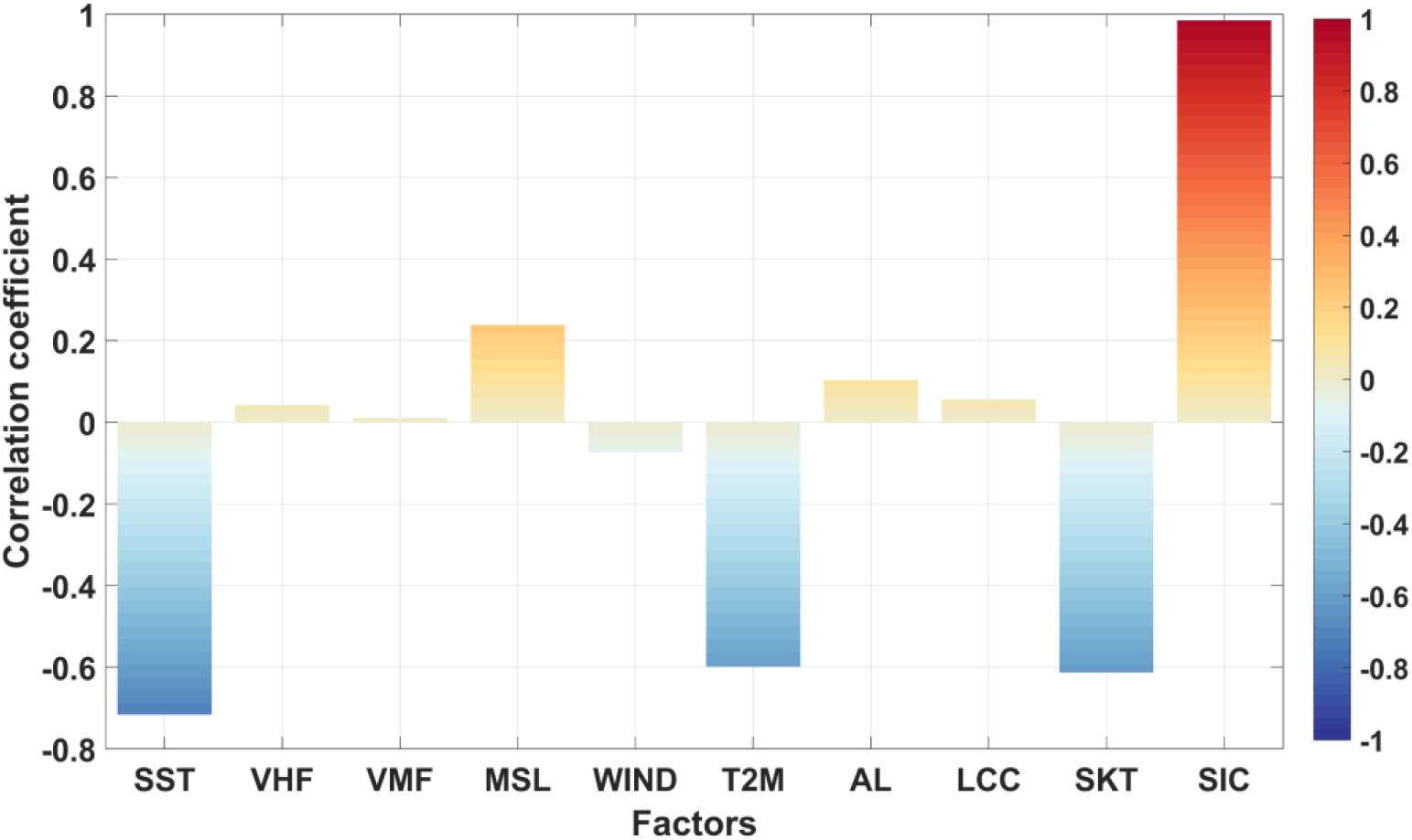
Figure 1. Time lag correlation coefficient of each factor. The intensity of warmer and cooler colors represents the magnitude of the time lag correlation.

As shown in Figure 1, the stronger the intensity of the warmer color, the greater the positive time lag correlation between this factor and SIC. The stronger the intensity of the cooler color, the greater the negative time lag correlation. Therefore, according to the absolute value of the time lag correlation, we non-dimensionalize the data of the five above-mentioned factors and normalize each one to between 0 and 100 to train the model. Due to missing land values in SST and SIC, nan values should not exist in the model training. Therefore, the nan values of land in the SST are set to -100 to clearly distinguish from sea surface temperature. The nan values of the land in SIC are set to 0 due to the absence of sea ice.

Data from January 2010 to December 2019 are used as the training set for the SIC prediction model, and data from January to December 2020 are used as test values of the model prediction effect. The longitude and latitude range from 120° to 180°E and 66.75° to 83°N, respectively.

Methods

This study was based on Grad-loss and applied ConvLSTM and PredRNN++ to 10 consecutive days of short-term daily SIC prediction. In addition to comparing the ConvLSTM and PredRNN++ models, this study also compared the prediction effects of different loss functions.

Convolutional Long Short-Term Memory Network

Convolutional long short-term memory network is a combination of CNNs and LSTM. CNNs are neural networks that include convolution calculations and are suitable for processing two-dimensional spatial field information. CNNs overcome the limitations of point-by-grid calculations and are mostly used in image recognition and classification fields (LeCun et al., 1998; Ren et al., 2017; Yoo et al., 2019). LSTM is a time-cycle neural network based on recurrent neural networks (RNNs) that processes time-series information. LSTM solves the long-term dependency problem of RNNs and has recently been used in speech recognition and text translation (Sundermeyer et al., 2015; Wang et al., 2020). ConvLSTM adds the convolution operation of CNNs based on LSTM and processes temporal and spatial field information (Shi et al., 2015). Therefore, ConvLSTM is more suitable for applications for image processing (Hu et al., 2020).

Improved Predictive Recurrent Neural Network

Predictive recurrent neural network is a deep learning network based on ConvLSTM. Principal improvements include changing the ConvLSTM neural unit to causal LSTM and proposing a new neural unit (Gradient Highway Unit, GHU). Causal LSTM calculates spatio-temporal information separately to better capture short-term dynamic changes. The GHU connects neural units at different moments and directly transmits characteristic historical information to subsequent moments. Thus, retaining the gradient during backpropagation is easier and partially solves the problem of gradient disappearance (Wang et al., 2018). PredRNN++ retains the advantages of ConvLSTM by processing time series and performing convolution operations on spatial fields. In addition, PredRNN++ is more suitable than ConvLSTM for predictions that rely on long-term historical sequences (Bonnet et al., 2020).

Gradient Loss Function

Most loss functions currently used in deep learning methods are mean square error loss function (MSE-loss) or mean absolute error loss function (MAE-loss). The calculation formulas of MSE-loss and MAE-loss are as follows:

$$MSE\_loss=\frac{1}{m}{\displaystyle \sum _{i=1}^m{\left(y_i-{\widehat{y}}_i\right)}^2}(1)$$

$$MSE\_loss=\frac{1}{m}{\displaystyle \sum _{i=1}^m\left|y_i-{\widehat{y}}_i\right|}(2)$$

Mean absolute error loss exhibits better robustness than MSE in the face of outliers, because MSE squares the error and gives outliers more weight. However, both MSE and MAE compare the real value with the predicted value grid by grid. Therefore, the MSE and MAE loss functions can only compare the difference between the real SIC and the predicted SIC at the same grid point in the network training process.

In fact, different oceanic regions respond differently to environmental factors. Thus, local sea ice changes also have an important impact on the prediction effect. Therefore, this study adopts a gradient based on MAE to reflect local sea ice changes, and proposes Grad-loss. We have compared the prediction effect when using MAE-loss and Grad-loss to explore the improvement of Grad-loss. The calculation formula for the Grad-loss is as follows:

$$\begin{array}{l}Gra{d}_{lat}=\left(y_{(i+1,j)}-y_{(i,j)}\right)-\left({\widehat{y}}_{(i+1,j)}-{\widehat{y}}_{(i,j)}\right)\\ \{\begin{array}{l}Gra{d}_{lon}=\left(y_{(i,j+1)}-y_{(i,j)}\right)-\left({\widehat{y}}_{(i,j+1)}-{\widehat{y}}_{(i,j)}\right)\\ Grad\_loss=\frac{1}{m}{\displaystyle \sum _{i=1}^m\left|y_i-{\widehat{y}}_i\right|}/std(y)*2+Gra{d}_{lat}/std(Gra{d}_{lat})+Gra{d}_{lon}/std(Gra{d}_{lon})\end{array}\end{array}(3)$$

where, Grad_lat and Grad_lon represent the gradients in the latitude and longitude directions, respectively; and std represents the standard deviation. To ensure that the dimensions of MAE and Grad are the same, the std of the SIC and the std of the gradient are removed from the formula.

Research Flow

This experiment builds ConvLSTM and PredRNN++ based on the TensorFlow deep learning environment (Abadi et al., 1983) and applies them to short-term SIC prediction.

Existing research on the sensitivity of network hyper-parameters shows that the prediction effect is better when the number of network layers is 3 (Wang et al., 2017). The layer of 3 strikes a balance between the modeling capability and data amount. A shallower model would lead to inadequate fitting and a deeper model cannot be effectively feeded. In the training phase, the training effect is better when the learning rate is set to 0.001 (Jun Kim et al., 2020). In this way, the loss can be reduced quickly, and the possibility of falling into a local optimum can be reduced. The kernel size of layer 1-3 is set 5-3, respectively. That is, the faster changes are extracted first, and then the subtle changes are learned (Jun Kim et al., 2020). The setting of filters, in a 3-layer network, usually decreases from 128 to 64. That is, the model extracts more changes in the front layer, and then gradually extracts the law related to sea ice change in the latter layer (Liu et al., 2021).

Consequently, three-layer networks are built for ConvLSTM and PredRNN++. The filters in each layer of the network were 128, 128, and 64, with kernel sizes of 5, 3, and 3, respectively. The dimension of input data was 4D (time series × height × width × factors). The batch size of input data was 32. The activation function was a rectified linear unit (ReLU). The optimizer used Adam, which combined the advantages of the AdaGrad and RMSProp optimization algorithms, had high computational efficiency, and required only a small amount of memory (Kingma and Ba, 2015). Table 1 presented the specific hyper-parameters.

TABLE 1

Table 1. ConvLSTM and PredRNN++ hyper-parameters.

Besides two different networks, two types of input data, and two types of loss functions are considered. The input data can be the SIC itself (namely the self-regression model), or the multiple factors listed in section “Factor Screening and Data Preprocessing.” These two cases are called single-factor and multi-factor hereinafter. In terms of loss function, a novel loss based on horizontal gradient (Grad-loss) is proposed, in order to improve the conventional MAE-loss. Eight models are thus constructed to make further comparison, as shown in Table 2.

TABLE 2

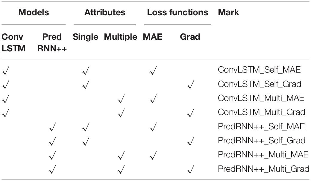
Table 2. SIC prediction model comparison experiment design.

The length of input sequence and output sequence can be an important factor of deep learning. The performance is usually better with the comparable length of input sequence and output sequence, but could be degraded with the former becoming longer (Wang et al., 2018; Bonnet et al., 2020; Liu et al., 2021).

The performance of each model is evaluated by the 10-day running test of 10-day lagged prediction in 2020. To be more specific, the prediction of January 11–20 is made by the data of January 1–10, succeeded by the prediction of January 12–21 from January 2–11, until the prediction of December 22–31. In this case, 347 seq-to-seq predictions are made in the year 2020. Figure 2 illustrated the analogy process.

FIGURE 2

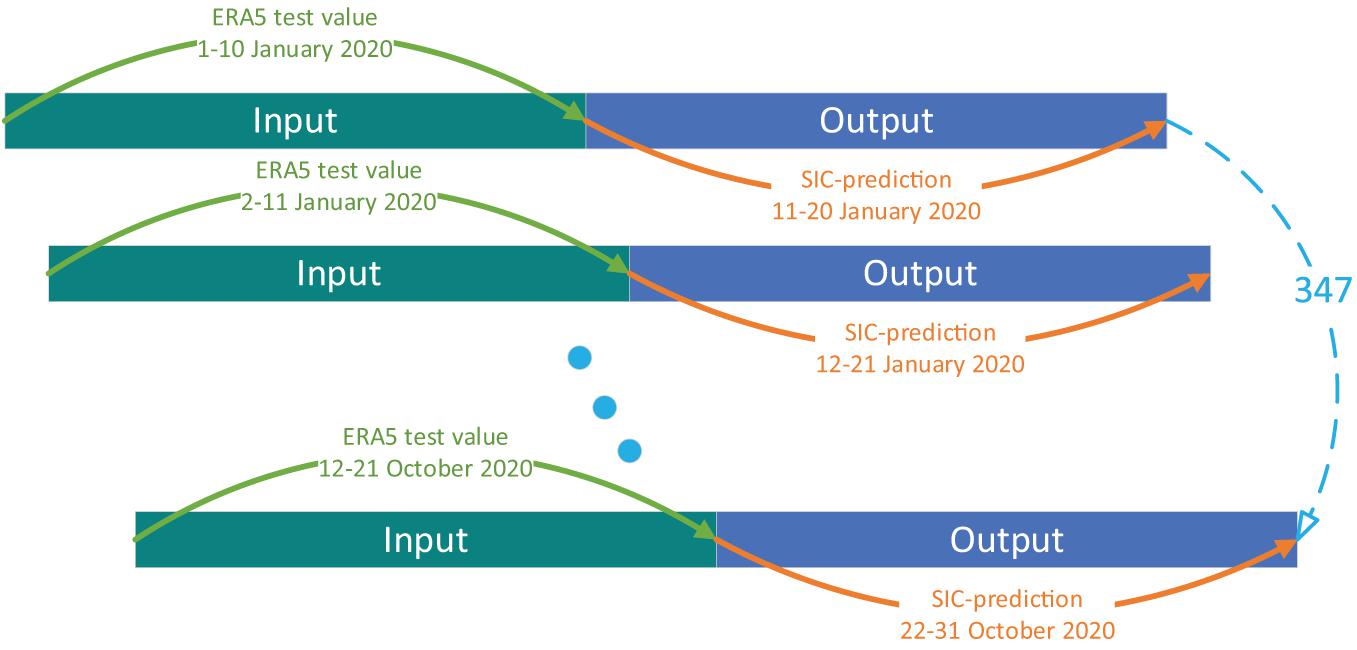
Figure 2. Date of model test input and output.

Based on a variety of properties of the human visual system, the spatial structure similarity (SSIM) considers the brightness, contrast, and structure information of the image. In deep learning, it is usually used to assess the quality of image prediction (Wang et al., 2004). Hence we have evaluated the SSIM, MAE, and the difference (DIFF) between the predicted value and the test value to compare the prediction effects of each model. The SSIM compares the spatial structure difference between the predicted value and the test value across the entire oceanic region; MAE compares the error of the two values in the overall oceanic region; the DIFF intuitively displays the difference of the error and the spatial distribution between the predicted and test values.

The DIFF and SSIM calculation methods are as follows:

$$DIFF=y-\widehat{y}(4)$$

$$SSIM(y,\widehat{y})=\frac{\left(2u_y{u}_{\widehat{y}}+c_1\right)\left(2{\sigma }_{y\widehat{y}}+c_2\right)}{\left(u_y^2+u_{\widehat{y}}^2+c_1\right)\left({\sigma }_y^2+{\sigma }_{\widehat{y}}^2+c_2\right)}(5)$$

where, u represents the average value, and σ represents the variance or covariance. c₁ and c₂ are constants, c₁ = (0.01^∗L)², and c₂ = (0.03^∗L)². L is set to 100 in this study to calculate SIC.

Figure 3 shows the oceanic region and control experiments designed in this study. Factor screening and pre-processing are adopted to generate the input datasets. Eight models are adopted for the training period (see Table 2). The test sets are put into the eight models to obtain their predictions. Three control experiments are designed to test the performance of the proposed multi-factor short-term daily SIC prediction model with three improvements, i.e., adopting multi-factors, gradient loss function and the advanced deep learning algorithm. Firstly, the impact of adopting multi-factors is tested by comparing the performance of single-factor and multi-factor both in ConvLSTM model and PredRNN++ model. Secondly, the impact of adopting gradient loss function is tested. Finally, the performance of adopting PredRNN++ model and ConvLSTM model are compared to showing the impact of advanced deep learning algorithm.

FIGURE 3

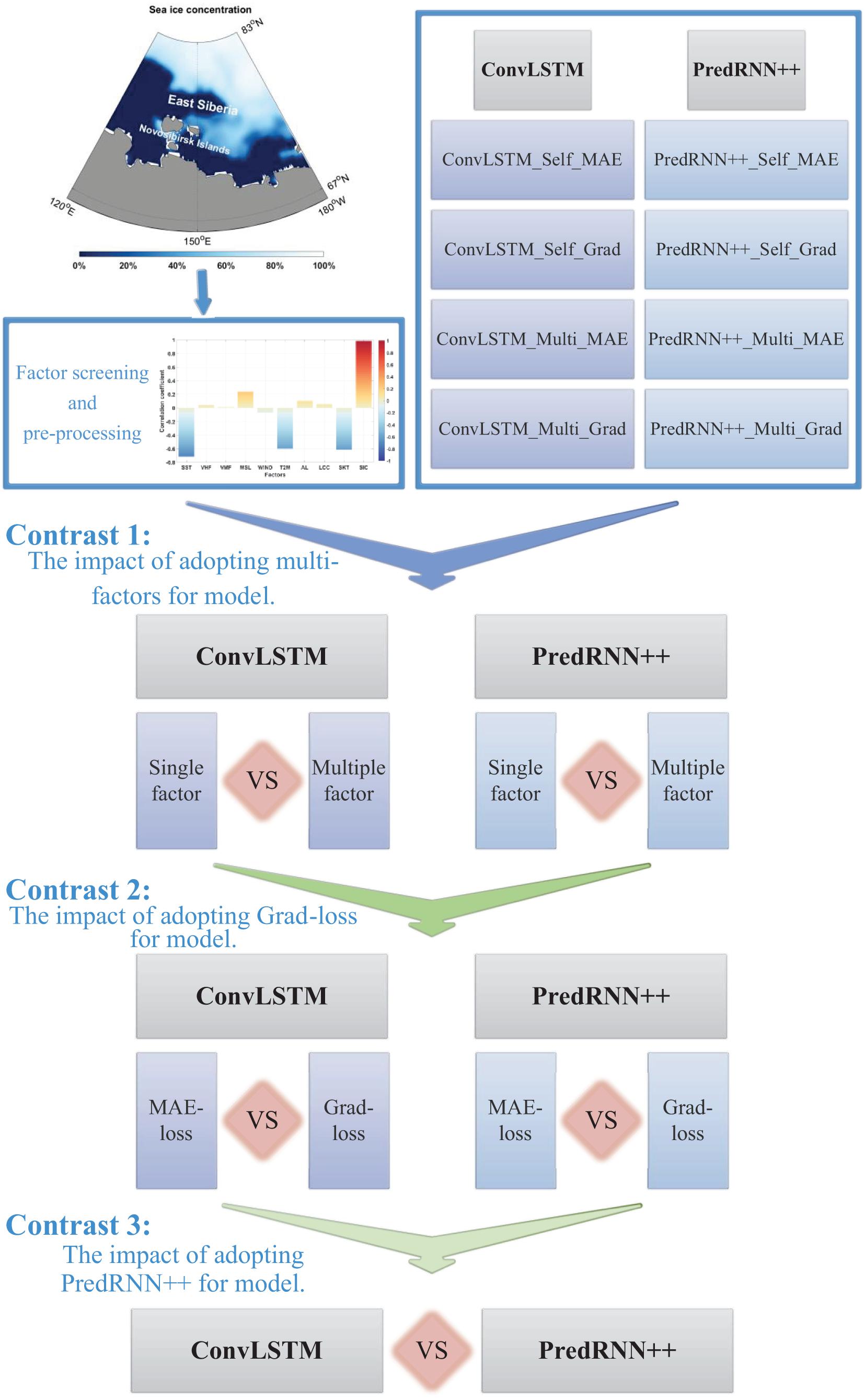
Figure 3. Model design and workflow schematic. Based on SSIM, MAE, and DIFF, the prediction effects of each model are compared in order.

Results and Discussion

Predictability

Although the above-mentioned models are used for 10-day SIC prediction during training, their effectiveness is unknown. Therefore, to test the predictability, we have compared the average MAE predicted by each model for 10 days with the monthly average MAE. Because the Northeast Passage is primarily navigable in autumn (September to November), we consider October as a comparison example. The monthly average SIC in October is subtracted from the daily SIC, and the monthly average MAE is obtained using formula 2.

Figure 4 shows that among the eight models, the model with the best prediction effect can reach 9 days of validity. That is to say, the prediction error on the 9th day is smaller than the monthly average change. Therefore, the follow-up comparison experiment between the SSIM and MAE of each model is conducted based on the longest predictable time (9 days).

FIGURE 4

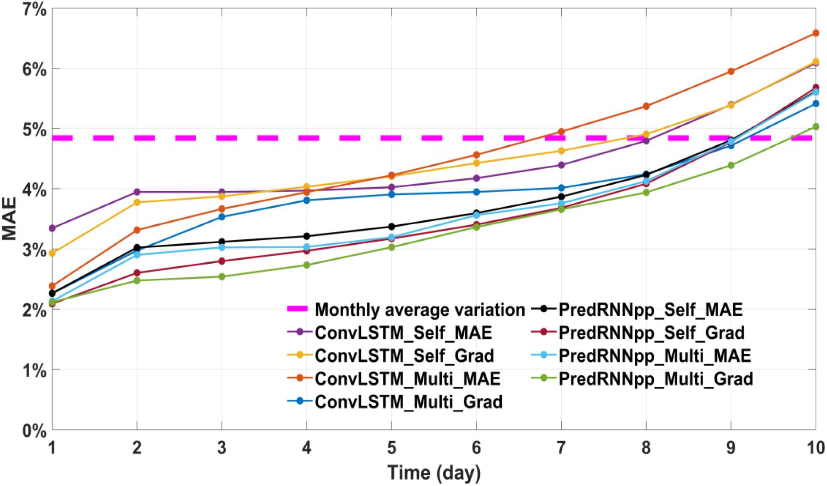
Figure 4. The magenta dashed line in the figure represents the monthly average MAE; the remaining 8 solid lines represent the average MAE of eight models for 10 consecutive days in October 2020.

Single Factor or Multiple Factors

This experiment uses the five factors selected in section “Factor Screening and Data Preprocessing” to verify whether the effect of multi-factor prediction is better than that of single-factor prediction. As shown in Figure 2, each model makes 347 10-day running predictions. Considering the validity cannot surpass 9 days (Figure 4), the SSIM and MAE of 347 consecutive 9-day predictions of each model are averaged over 9 days to compare the effects of predictions. Figures 5, 6 show the results.

FIGURE 5

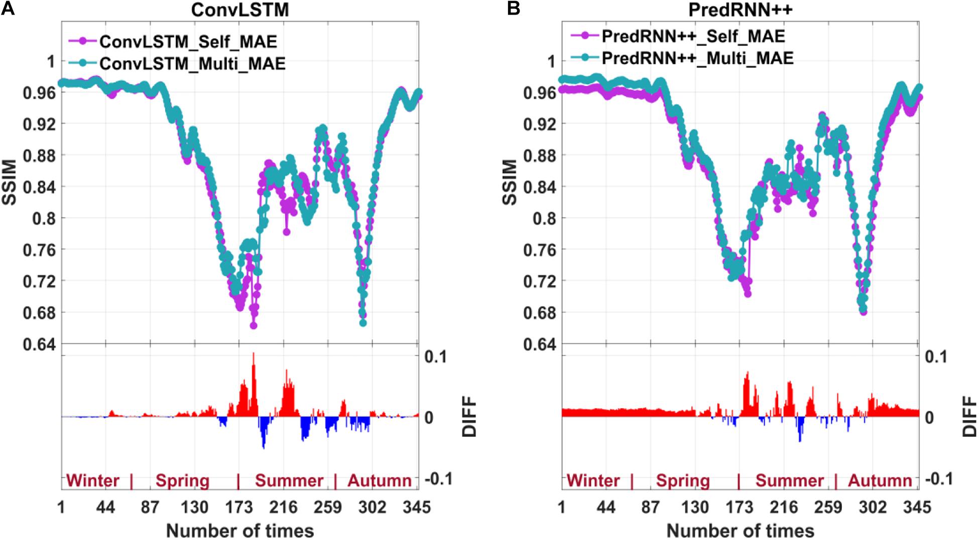
Figure 5. The SSIM for single-factor and multi-factor ConvLSTM predictions based on MAE-loss (A) and the SSIM for single-factor and multi-factor PredRNN++ predictions (B). The DIFF in the bar graph is obtained by subtracting the single-factor model from the multi-factor model. The red color represents the positive value, and the blue color represents the negative value.

FIGURE 6

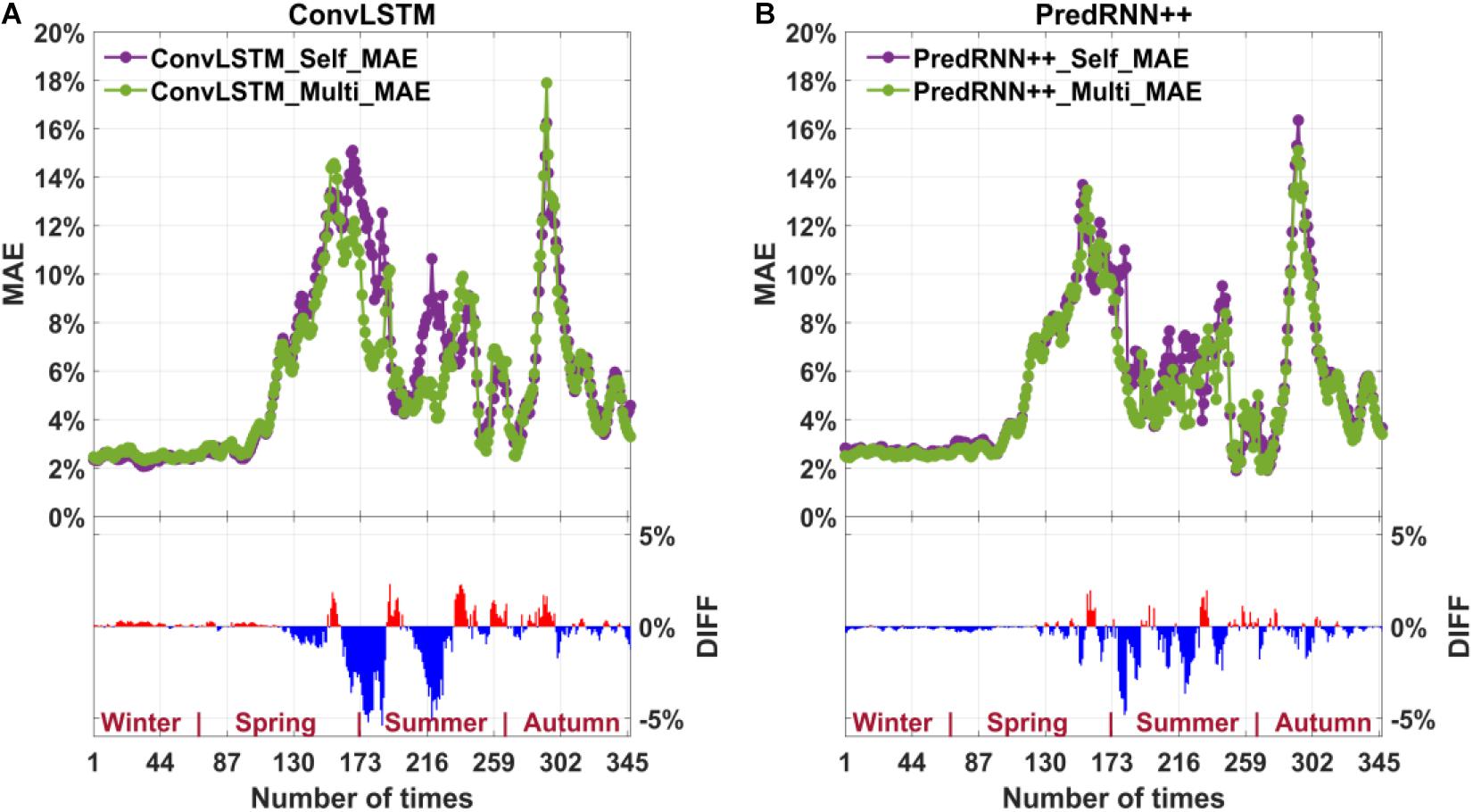
Figure 6. MAE for single-factor and multi-factor ConvLSTM predictions based on MAE-loss (A) and MAE for single-factor and multi-factor PredRNN++ predictions (B). The DIFF in the bar graph is obtained by subtracting the single-factor model from the multi-factor model. The red color represents the positive value, and the blue color represents the negative value.

In Figure 5, the positive value of DIFF indicates the better performance of multi-factor model. The performance of the multi-factor model in summer is sometimes less effective. But more often than not, multi-factor model has better spatial structure similarity. In Figure 6, the negative value of DIFF indicates the better performance of multi-factor model. In most cases, the error of the multi-factor model is smaller. In spring and summer, although there are fluctuations, the improvement effect is more obvious. Therefore, in general, the prediction effect of multi-factor model is better than that of single-factor model. The multi-factor improvement effect is more obvious on PredRNN++.

The advantage of the multi-factor prediction model over a single factor is primarily reflected in the season when the sea ice changes greatly. In summer, melt ponds change the albedo of the sea surface and decrease the accuracy of summer SIC observations (Cavalieri et al., 1990; Perovich et al., 2007; Mäkynen et al., 2014). Therefore, the multi-factor model is more accurate through considering the factors affecting sea ice to weaken the influence of melt ponds (Liu et al., 2021).

Mean Absolute Error-Loss or Gradient Loss Function

To test whether using Grad-loss can improve model prediction, we have divided the ConvLSTM and PredRNN++ multi-factor prediction model into two types: MAE-loss and Grad-loss. The SSIM and MAE of the prediction results are averaged for nine consecutive days. Figures 7, 8 show the results.

FIGURE 7

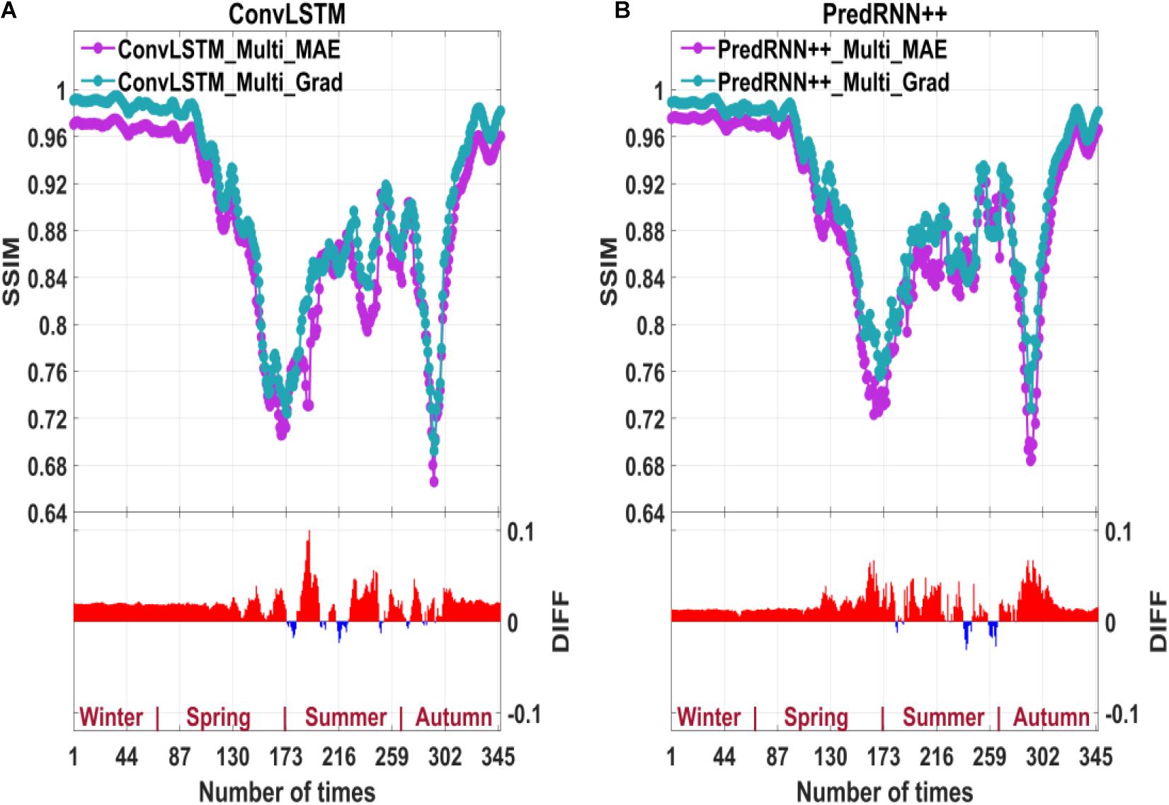
Figure 7. The SSIM for multi-factor prediction of ConvLSTM based on MAE-loss and Grad-loss (A); the SSIM for multi-factor prediction of PredRNN++ based on MAE-loss and Grad-loss (B). The DIFF in the bar graph is obtained by subtracting the model based on MAE-loss from the model based on Grad-loss.

FIGURE 8

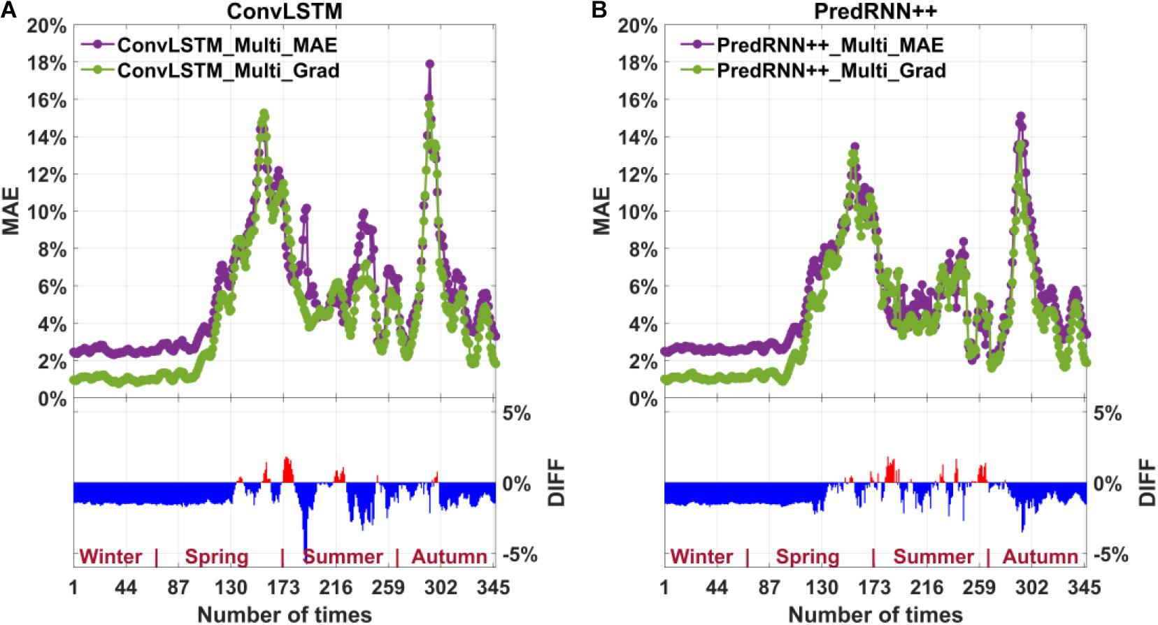
Figure 8. MAE for the multi-factor prediction of ConvLSTM based on MAE-loss and Grad-loss (A); MAE for the multi-factor prediction of PredRNN++ based on MAE-loss and Grad-loss (B). The DIFF in the bar graph is obtained by subtracting the model based on MAE-loss from the model based on Grad-loss.

Figures 7, 8 show that Grad-loss further improves the accuracy of the SIC prediction model based on multiple factors for ConvLSTM and PredRNN++. Grad-loss adds the local change of SIC to the loss function by considering the gradient between adjacent grid points. Thus, the Grad-loss-based SIC prediction model considering local SIC changes produces more accurate predictions than the MAE-loss-based model. In addition, Grad-loss significantly improves year-round prediction accuracy (rather than only in the summer).

Convolutional Long Short-Term Memory Network or Improved Predictive Recurrent Neural Network

According to model differences, this experiment has divided into two categories to test the applicability of the ConvLSTM and PredRNN++ for short-term SIC prediction. In addition to taking the 9-day average of the SSIM and MAE, this study also averages 347 prediction results for nine consecutive days. The average effects of 347 predictions and consecutive 9-day predictions are compared. Figures 9, 10 compare the model prediction results.

FIGURE 9

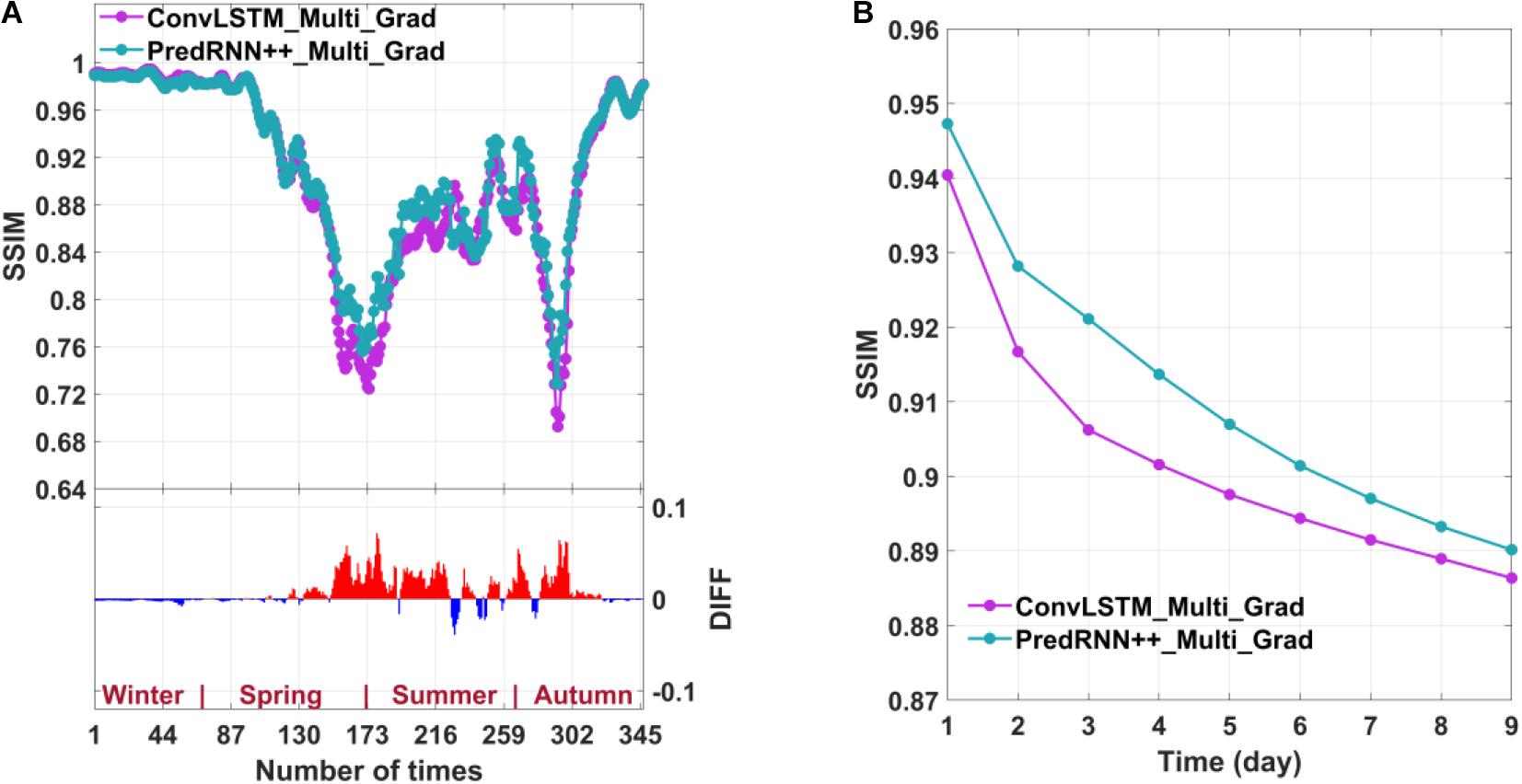
Figure 9. Average SSIM for the ConvLSTM and PredRNN++ multi-factor models for 347 predictions (A); Average SSIM of the nine consecutive days of prediction (B). The DIFF in the bar graph is obtained by subtracting the model of ConvLSTM from the model of PredRNN++.

FIGURE 10

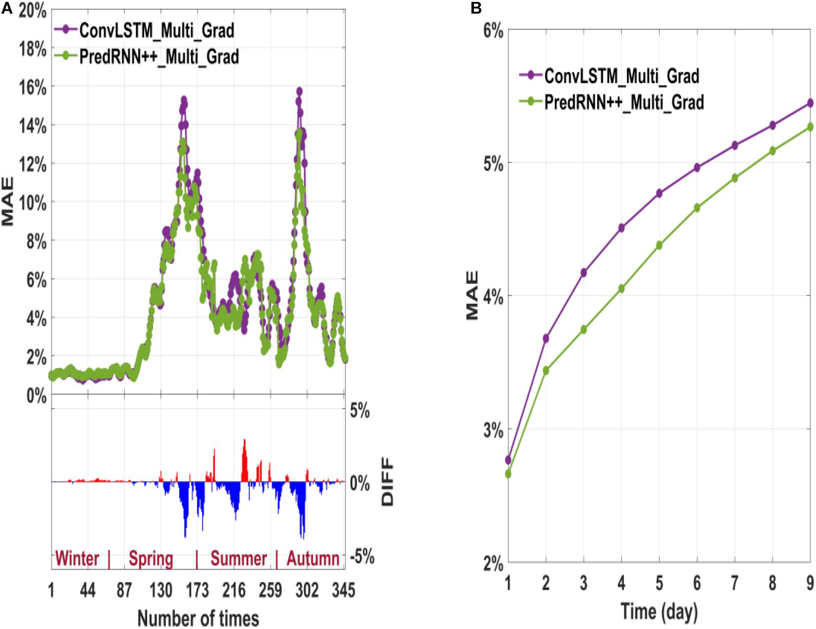
Figure 10. Average MAE of the ConvLSTM and PredRNN++ multi-factor models in 347 predictions (A); The average MAE of the nine consecutive days of prediction (B). The DIFF in the bar graph is obtained by subtracting the model of ConvLSTM from the model of PredRNN++.

Figures 9, 10 show that the PredRNN++ multi-factor prediction model based on Grad-loss has a relatively high SSIM and low MAE. The advantage of PredRNN++ over ConvLSTM for the 347 predictions is primarily reflected in seasons with significant sea ice changes. PredRNN++ produces the best 9-day prediction results.

In addition to comparing the SSIM and MAE of the entire oceanic region, this study also has compared the size and distribution of the DIFF of the two types of models in the spatial field. Because Arctic sea ice changes greatly in summer (June to August), this study has calculated the DIFF between the predicted and test values in July 2020. Owing to the different predictability of different models, this study only compares the first-day prediction results. Figure 11 shows the 15 July prediction results.

FIGURE 11

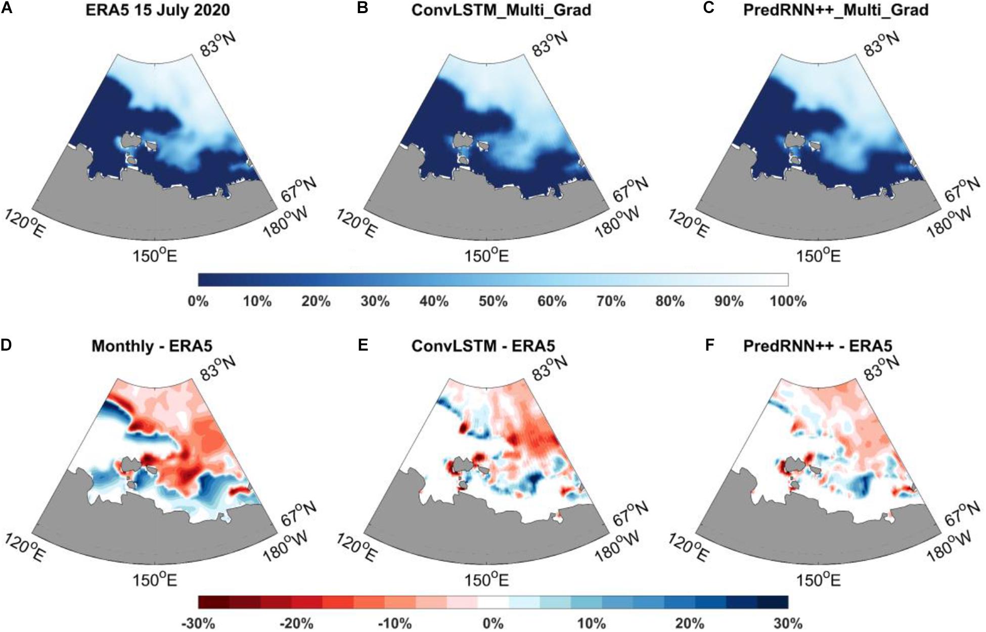
Figure 11. The SIC of ERA5 in the East Siberian Sea on 15 July 2020 (A). The SIC predicted by ConvLSTM on 15 July (B). The SIC predicted by PredRNN++ on 15 July (C). The DIFF of the monthly average SIC minus (A) in July (D). The DIFF of the (B) minus (A,E). The DIFF of the (C) minus (A,F).

Figure 11 shows that the DIFF of the monthly average result is the largest, indicating significant SIC variability in the current month. Overall, the DIFF of the PredRNN++ multi-factor prediction model based on Grad-loss is the smallest. In addition, the DIFF spatial distribution of the PredRNN++ model is relatively uniform, with no large-scale oceanic region deviations. Except for large deviations near islands, deviations in most oceanic regions are below 10%. By comparison, ConvLSTM has large deviations oceanic regions and a relatively large overall deviation.

The SSIM, MAE, and DIFF indicators show that the PredRNN++ multi-factor prediction model based on Grad-loss has the best prediction effect. The prediction effect of the Grad-loss-based ConvLSTM multi-factor model is similar to that of PredRNN++ in winter but inferior during periods of significant SIC changes (summer and autumn). Summer and autumn are the navigable seasons of the Northeast Passage, and the East Siberian Sea is an essential sea of the Northeast Passage (Kunkel, 2004). Thus, the requirements for sea ice prediction are higher and the PredRNN++ multi-factor prediction model based on Grad-loss is the best choice.

Models trained by PredRNN++ had better prediction results than those of ConvLSTM primarily due to the improved Causal LSTM in PredRNN++. The Causal LSTM could separately calculate temporal and spatial change of the unit by adding more non-linear calculations under the same network level condition. Thus, it could better reflect SIC variation in summer and autumn. However, more non-linear calculations in PredRNN++ might not significantly improve the results in winter as the little SIC change.

The PredRNN++ multi-factor prediction model based on Grad-loss had the highest prediction skill but still had some limitations. First, the SST and SIC land missing values were set to -100 and 0, respectively, causing the training data to deviate from the true physical meaning. In the future, an attention mechanism could possibly be introduced to concentrate the weight of the convolution calculation on the sea ice region and to weaken the influence of the missing values. Second, PredRNN++ made longer predictions and achieved higher accuracy but sharply increased network complexity and computational overhead. The computational cost of PredRNN++ was more than twice that of ConvLSTM. Follow-up work might be able to simplify the PredRNN++ network structure to reduce the computational cost while ensuring the SIC prediction effect.

In addition, the predictability of the model for Arctic navigation had an important influence on trajectory planning results. Longer model predictions could produce more extensive area predictions with the trajectory planning algorithm and reduce the likelihood of falling into a local optimum (Koenig and Likhachev, 2005). The MAE of continuous 9-day prediction showed that the Grad-loss-based PredRNN++ multi-factor prediction model had the slowest error increase and the smallest error range among the models. Therefore, the PredRNN++ multi-factor prediction model based on Grad-loss was more suitable for trajectory planning in Arctic waters.

Conclusion

Model numerical simulation is based on known laws, which has a time-consuming calculation. This study has proposed a new predict model with adopting multiple factors, gradient loss function and an advanced deep learning algorithm called PredRNN++ that can continuously predict daily SIC for up to 9 days. Factor screening is adopted to select 5 of 10 factors that affected SIC changes for prediction. Three control experiments are designed to test the impact of these three improvements for model performance.

Additionally, the SSIM, MAE, and DIFF indicators are used to evaluate the prediction effect of each model, and the following conclusions are drawn:

1. The physical interpretation of the prediction models and the short-term SIC prediction effect are improved by introducing multiple factors related to SIC changes.

2. Grad-loss function further improves the accuracy of daily SIC prediction of the multi-factor model by adding extra information of local SIC variation.

3. The PredRNN++ multi-factor prediction model based on Grad-loss function has the best spatial structure similarity, the lowest error, and the best predictability. Additionally, the PredRNN++ model has the smallest deviation between the predicted value and the test value and contains no large-scale oceanic region deviations.

Data Availability Statement

The original contributions presented in the study are included in the article/supplementary material, further inquiries can be directed to the corresponding author.

Author Contributions

QL: methodology, validation, writing—original draft preparation, and visualization. RZ: conceptualization, validation, project administration, and funding acquisition. YW: validation, formal analysis, resources, and supervision. HY: methodology and visualization. MH: data curation and funding acquisition. All authors contributed to the article and approved the submitted version.

Funding

This study was supported by the National Natural Science Foundation of China (Nos. 41976188 and 41875061).

Conflict of Interest

The authors declare that the research was conducted in the absence of any commercial or financial relationships that could be construed as a potential conflict of interest.

Publisher’s Note

All claims expressed in this article are solely those of the authors and do not necessarily represent those of their affiliated organizations, or those of the publisher, the editors and the reviewers. Any product that may be evaluated in this article, or claim that may be made by its manufacturer, is not guaranteed or endorsed by the publisher.

References

Abadi, M., Paul, B., Jianmin, C., Zhifeng, C., Andy, D., and Jeffrey, D. (1983). TensorFlow: a system for large-scale machine learning. Methods Enzymol. 101, 582–598. doi: 10.1016/0076-6879(83)01039-1033

CrossRef Full Text | Google Scholar

Auligné, T., McNally, A. P., and Dee, D. P. (2007). Adaptive bias correction for satellite data in a numerical weather prediction system. Q. J. R. Meteorol. Soc. 133, 631–642. doi: 10.1002/QJ.56

CrossRef Full Text | Google Scholar

Ballinger, T. J., and Sheridan, S. C. (2015). Regional atmospheric patterns and the delayed sea-ice freeze-up in the western Arctic. Clim. Change 131, 229–243. doi: 10.1007/S10584-015-1383-1385

CrossRef Full Text | Google Scholar

Bonnet, S. M., Evsukoff, A., and Rodriguez, C. A. M. (2020). Precipitation nowcasting with weather radar images and deep learning in são paulo, brasil. Atmosphere (Basel) 11:1157. doi: 10.3390/atmos11111157

CrossRef Full Text | Google Scholar

Bormann, N., Fouilloux, A., and Bell, W. (2013). Evaluation and assimilation of ATMS data in the ECMWF system. J. Geophys. Res. Atmos. 118, 12 970–12 980. doi: 10.1002/2013JD020325

CrossRef Full Text | Google Scholar

Cavalieri, D. J., Burns, B. A., and Onstott, R. G. (1990). Investigation of the effects of summer melt on the calculation of sea ice concentration using active and passive microwave data. J. Geophys. Res. 95, 5359–5369. doi: 10.1029/JC095iC04p05359

CrossRef Full Text | Google Scholar

Chen, J., Kang, S., Chen, C., You, Q., Du, W., Xu, M., et al. (2020). Changes in sea ice and future accessibility along the Arctic Northeast Passage. Glob. Planet. Change 195:103319. doi: 10.1016/j.gloplacha.2020.103319

CrossRef Full Text | Google Scholar

Chi, J., and Kim, H. C. (2017). Prediction of Arctic sea ice concentration using a fully data driven deep neural network. Remote Sens. 9:1305. doi: 10.3390/rs9121305

CrossRef Full Text | Google Scholar

Comiso, J. C., Gersten, R. A., Stock, L. V., Turner, J., Perez, G. J., and Cho, K. (2017). Positive trend in the Antarctic sea ice cover and associated changes in surface temperature. J. Clim. 30, 2251–2267. doi: 10.1175/JCLI-D-16-0408.1

PubMed Abstract | CrossRef Full Text | Google Scholar

Cox, C. J., Uttal, T., Long, C. N., Stone, R. S., Shupe, M. D., and Starkweather, S. (2016). The role of springtime arctic clouds in determining autumn sea ice extent. J. Clim. 29, 6581–6596. doi: 10.1175/JCLI-D-16-0136.1

CrossRef Full Text | Google Scholar

Francis, J. A., and Vavrus, S. J. (2015). Evidence for a wavier jet stream in response to rapid Arctic warming. Environ. Res. Lett. 10:014005. doi: 10.1088/1748-9326/10/1/014005

CrossRef Full Text | Google Scholar

Gu, S., Zhang, Y., Wu, Q., and Yang, X.-Q. (2018). The linkage between arctic sea ice and midlatitude weather: in the perspective of energy. J. Geophys. Res. 123, 536–511. doi: 10.1029/2018JD028743

CrossRef Full Text | Google Scholar

Guemas, V., Blanchard-Wrigglesworth, E., Chevallier, M., Day, J. J., Déqué, M., Doblas-Reyes, F. J., et al. (2016). A review on Arctic sea-ice predictability and prediction on seasonal to decadal time-scales. Q. J. R. Meteorol. Soc. 142, 546–561. doi: 10.1002/qj.2401

CrossRef Full Text | Google Scholar

Hersbach, H., Bell, B., Berrisford, P., Biavati, G., Horányi, A., Muñoz Sabater, J., et al. (2018). ERA5 hourly data on single levels from 1979 to present. Copernicus Clim. Chang. Serv. Clim. Data Store doi: 10.24381/cds.adbb2d47

CrossRef Full Text | Google Scholar

Hersbach, H., Bell, B., Berrisford, P., Hirahara, S., Horányi, A., Muñoz-Sabater, J., et al. (2020). The ERA5 global reanalysis. Q. J. R. Meteorol. Soc. 146, 1999–2049. doi: 10.1002/qj.3803

CrossRef Full Text | Google Scholar

Hu, W. S., Li, H. C., Pan, L., Li, W., Tao, R., and Du, Q. (2020). Spatial-Spectral feature extraction via deep ConvLSTM neural networks for hyperspectral image classification. IEEE Trans. Geosci. Remote Sens. 58, 4237–4250. doi: 10.1109/TGRS.2019.2961947

CrossRef Full Text | Google Scholar

Hunke, E. C., Lipscomb, W. H., and Turner, A. K. (2011). Sea-ice models for climate study: retrospective and new directions. J. Glaciol. 56, 1162–1172. doi: 10.3189/002214311796406095

CrossRef Full Text | Google Scholar

Hunke, E. C., Lipscomb, W. H., Turner, A. K., Jeffery, N., and Elliott, S. (2013). CICE: the Los Alamos Sea Ice Model Documentation and Software User’s Manual Version 4.0 LA-CC-06-012.

Google Scholar

Jun Kim, Y., Kim, H. C., Han, D., Lee, S., and Im, J. (2020). Prediction of monthly Arctic sea ice concentrations using satellite and reanalysis data based on convolutional neural networks. Cryosphere 14, 1083–1104. doi: 10.5194/tc-14-1083-2020

CrossRef Full Text | Google Scholar

Kingma, D. P., and Ba, J. L. (2015). “Adam: a method for stochastic optimization,” in Proceedings of the 3rd International Conference on Learning Representations, ICLR 2015 - Conference Track Proceedings, (San Diego).

Google Scholar

Koenig, S., and Likhachev, M. (2005). Fast replanning for navigation in unknown terrain. IEEE Trans. Robot. 21, 354–363. doi: 10.1109/TRO.2004.838026

CrossRef Full Text | Google Scholar

Kunkel, C. (2004). Essen im laufe der jahreszeiten: der herbst. Akupunkt. Tradit. Chinesische Medizin 32, 155–156.

Google Scholar

LeCun, Y., Bottou, L., Bengio, Y., and Haffner, P. (1998). Gradient-based learning applied to document recognition. Proc. IEEE 86, 2278–2323. doi: 10.1109/5.726791

CrossRef Full Text | Google Scholar

Lee, H. J., Kwon, M. O., Yeh, S. W., Kwon, Y. O., Park, W., Park, J. H., et al. (2017). Impact of poleward moisture transport from the North Pacific on the acceleration of sea ice loss in the Arctic since 2002. J. Clim. 30, 6757–6769. doi: 10.1175/JCLI-D-16-0461.1

CrossRef Full Text | Google Scholar

Liu, Q., Zhang, R., Wang, Y., Yan, H., and Hong, M. (2021). Daily prediction of the arctic sea ice concentration using reanalysis data based on a convolutional LSTM network. J. Mar. Sci. Eng. 9:330. doi: 10.3390/jmse9030330

CrossRef Full Text | Google Scholar

Mahmoodi, K., Ghassemi, H., and Razminia, A. (2019). Temporal and spatial characteristics of wave energy in the Persian Gulf based on the ERA5 reanalysis dataset. Energy 187:115991. doi: 10.1016/j.energy.2019.115991

CrossRef Full Text | Google Scholar

Mäkynen, M., Kern, S., Rösel, A., and Pedersen, L. T. (2014). On the estimation of melt pond fraction on the arctic sea ice with ENVISAT WSM images. IEEE Trans. Geosci. Remote Sens. 52, 7366–7379. doi: 10.1109/TGRS.2014.2311476

CrossRef Full Text | Google Scholar

Mudryk, L. R., Derksen, C., Howell, S., Laliberté, F., Thackeray, C., Sospedra-Alfonso, R., et al. (2018). Canadian snow and sea ice: historical trends and projections. Cryosphere 12, 1157–1176. doi: 10.5194/tc-12-1157-2018

CrossRef Full Text | Google Scholar

Muhammed Naseef, T., and Sanil Kumar, V. (2020). Climatology and trends of the Indian Ocean surface waves based on 39-year long ERA5 reanalysis data. Int. J. Climatol. 40, 979–1006. doi: 10.1002/joc.6251

CrossRef Full Text | Google Scholar

Perovich, D. K., Nghiem, S. V., Markus, T., and Schweiger, A. (2007). Seasonal evolution and interannual variability of the local solar energy absorbed by the Arctic sea ice-ocean system. J. Geophys. Res. Ocean. 112, 1–13. doi: 10.1029/2006JC003558

CrossRef Full Text | Google Scholar

Ren, S., He, K., Girshick, R., and Sun, J. (2017). Faster R-CNN: towards real-time object detection with region proposal networks. IEEE Trans. Pattern Anal. Mach. Intell. 39, 1137–1149. doi: 10.1109/TPAMI.2016.2577031

PubMed Abstract | CrossRef Full Text | Google Scholar

Screen, J. A., and Simmonds, I. (2010). The central role of diminishing sea ice in recent Arctic temperature amplification. Nature 464, 1334–1337. doi: 10.1038/nature09051

PubMed Abstract | CrossRef Full Text | Google Scholar

Shi, X., Chen, Z., Wang, H., Yeung, D. Y., Wong, W. K., and Woo, W. C. (2015). Convolutional LSTM network: a machine learning approach for precipitation nowcasting. Adv. Neural Inf. Process. Syst. 2015, 802–810.

Google Scholar

Similä, M., and Lensu, M. (2018). Estimating the speed of ice-going ships by integrating SAR imagery and ship data from an automatic identification system. Remote Sens. 10:1132. doi: 10.3390/rs10071132

CrossRef Full Text | Google Scholar

Stroeve, J. C., Serreze, M. C., Holland, M. M., Kay, J. E., Malanik, J., and Barrett, A. P. (2012). The Arctic’s rapidly shrinking sea ice cover: a research synthesis. Clim. Change 110, 1005–1027. doi: 10.1007/s10584-011-0101-1

CrossRef Full Text | Google Scholar

Sundermeyer, M., Ney, H., and Schluter, R. (2015). From feedforward to recurrent LSTM neural networks for language modeling. IEEE Trans. Audio Speech Lang. Process. 23, 517–529. doi: 10.1109/TASLP.2015.2400218

CrossRef Full Text | Google Scholar

Tseng, P. H., Zhou, A., and Hwang, F. J. (2021). Northeast passage in Asia-Europe liner shipping: an economic and environmental assessment. Int. J. Sustain. Transp. 15, 273–284. doi: 10.1080/15568318.2020.1741747

CrossRef Full Text | Google Scholar

Vancoppenolle, M., Fichefet, T., Goosse, H., Bouillon, S., Madec, G., and Maqueda, M. A. M. (2009). Simulating the mass balance and salinity of Arctic and Antarctic sea ice. 1. Model description and validation. Ocean Model. 27, 33–53. doi: 10.1016/j.ocemod.2008.10.005

CrossRef Full Text | Google Scholar

Wang, L., Scott, K. A., and Clausi, D. A. (2017). Sea ice concentration estimation during freeze-up from SAR imagery using a convolutional neural network. Remote Sens. 9:408. doi: 10.3390/rs9050408

CrossRef Full Text | Google Scholar

Wang, L., Yuan, X., and Li, C. (2019). Subseasonal forecast of Arctic sea ice concentration via statistical approaches. Clim. Dyn. 52, 4953–4971. doi: 10.1007/s00382-018-4426-4426

CrossRef Full Text | Google Scholar

Wang, R., Luo, H., Wang, Q., Li, Z., Zhao, F., and Huang, J. (2020). A spatial-temporal positioning algorithm using residual network and LSTM. IEEE Trans. Instrum. Meas. 69, 9251–9261. doi: 10.1109/TIM.2020.2998645

CrossRef Full Text | Google Scholar

Wang, Z., Bovik, A. C., Sheikh, H. R., and Simoncelli, E. P. (2004). Image quality assessment: from error visibility to structural similarity. IEEE Trans. Image Process. 13, 600–612. doi: 10.1109/TIP.2003.819861

PubMed Abstract | CrossRef Full Text | Google Scholar

Wang, Y., Gao, Z., Long, M., Wang, J., and Yu, P. S. (2018). “PredRNN++: towards a resolution of the deep-in-time dilemma in spatiotemporal predictive learning,” in Proceedings of the 35th International Conference on Machine Learning, ICML 2018. (Stockholm, Sweden).

Google Scholar

Yoo, C., Han, D., Im, J., and Bechtel, B. (2019). Comparison between convolutional neural networks and random forest for local climate zone classification in mega urban areas using Landsat images. ISPRS J. Photogramm. Remote Sens. 157, 155–170. doi: 10.1016/j.isprsjprs.2019.09.009

CrossRef Full Text | Google Scholar