 Hao Liu
 Zexun Wei
 Ingo Richter4
 Chuanshun Li
- 1First Institute of Oceanography, Ministry of Natural Resources, Qingdao, China
- 2Laboratory for Regional Oceanography and Numerical Modelling, Pilot National Laboratory for Marine Science and Technology, Qingdao, China
- 3Shandong Key Laboratory of Marine Science and Numerical Modelling, Qingdao, China
- 4Application Laboratory, Research Institute for Value-Added-Information Generation, Japan Agency for Marine-Earth Science and Technology, Yokohama, Japan
The North Brazil Undercurrent (NBUC) is a narrow (<1°) northward western boundary current in the tropical South Atlantic Ocean. It carries a large volume of water (>16 Sv) and plays an important role in the Atlantic Meridional Overturning Circulation and the South Atlantic Subtropical Cell. Strong salinity and temperature fronts occur over the NBUC region. The role of temperature and salinity gradients on the genesis of NBUC variability has never been explored. This study uses three high-resolution (≤0.1°) and one low-resolution (=0.25°) model outputs to explore the linear trend of NBUC transport and its variability on annual and interannual time scales. We find that the linear trend and interannual variability of the geostrophic NBUC transport show large discrepancies among the datasets. Thus, the linear trend and variability of the geostrophic NBUC are associated with model configuration. We also find that the relative contributions of salinity and temperature gradients to the geostrophic shear of the NBUC are not model dependent. Salinity-based and temperature-based geostrophic NBUC transports tend to be opposite-signed on all time scales. Despite the limited salinity and temperature profiles, the model results are consistent with the in-situ observations on the annual cycle and interannual time scales. This study shows the relationship of salinity-based and temperature-based geostrophic NBUC variations in the annual and interannual variability and trend among different models and highlights the equal important roles of temperature and salinity in driving the variability of NBUC transport.
Introduction
The western tropical South Atlantic is a key conduit of the Atlantic Meridional Overturning Circulation (AMOC, Garzoli and Matano, 2011), involving a deep southward flow of cold and salty North Atlantic Deep Water (NADW) and compensating northward flows (Figures 1A,B) above the NADW. In the climatological mean flow fields off the eastern portion of the North Brazilian coast, the surface flow has a weak northward or even southward expression (Figure 1B) due to the toward shore Ekman drift (Figure 12 from da Silveira et al., 1994). In the Southern Hemisphere, the westward zonal wind stress drives the southward coastal current, which attenuates or conceals the northward geostrophic currents (Stramma et al., 1995). Below the surface and above the NADW, the flow is northward, and the maximum velocity core is at approximately 200 m with the magnitude estimated between 0.5 m/s (da Silveira et al., 1994) and 1 m/s (Dossa et al., 2021). The subsurface current between 5 and 11°S is called the North Brazil Undercurrent (NBUC, Figures 1A,B). At approximately 4.8°S, the NBUC merges with the central South Equatorial Current (a surface strengthened flow, Dossa et al., 2021), forming the North Brazil Current (NBC).
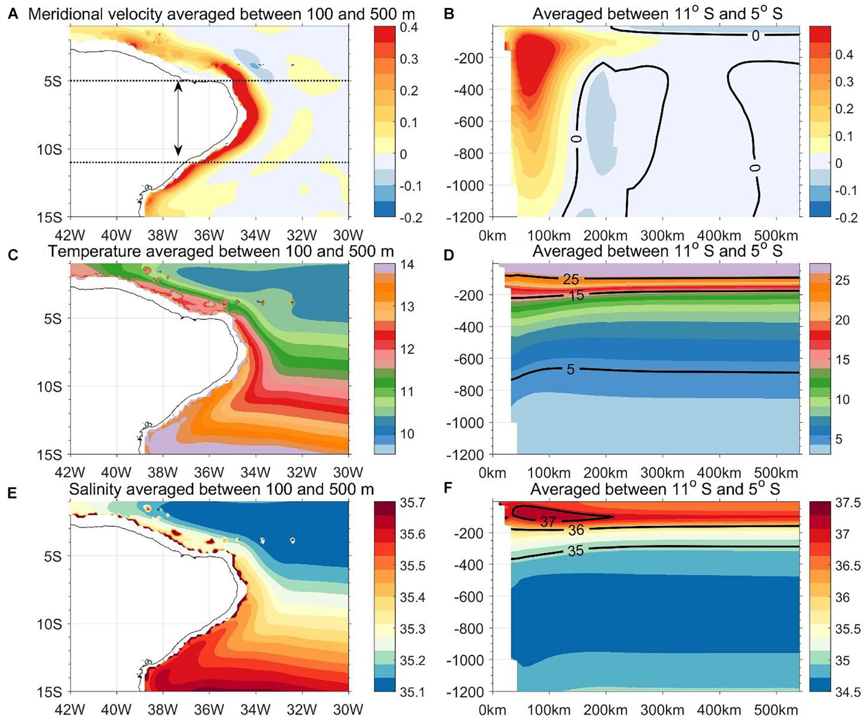
Figure 1. Horizontal and vertical sections of (A,B) the meridional velocity, (C,D) conservative temperature, and (E,F) absolute salinity. The variables shown in the horizontal sections are averaged between 100 and 500 m by a depth-weighted method with variables on a regular 5 m intervals. The variables shown in the distance-depth sections are averaged between 11 and 5°S. The x-axis in panels (B,D,F) is defined as the distance from the sea surface coast. The dotted lines in panel (A) mark the 11 and 5°S zonal lines. The solid lines in panels (A,C,E) are the coastline. The solid lines in panels (B,D,F) are the zero velocity, isotherms from 5 to 25°C, and isohalines from 35 to 37 g/kg, respectively. The meridional velocity, temperature, and salinity are derived from the ensemble mean of three high-resolution models (including GLORYS12V1, OFES2, and HYCOM). The units for velocity are m/s, for temperature are °C, and for salinity are g/kg.
The NBUC originates from the southern South Equatorial Current (sSEC; da Silveira et al., 1994; Stramma and England, 1999). It encounters the Brazilian coast at the southern sections of the 11°S zonal line, where it deflects in the south and north directions. The one deflected toward the equator (Rodrigues et al., 2007) is the NBUC. Between 11 and 4.8°S, the NBUC is generally confined between the sea surface and the upper Circumpolar Deep Water (uCDW; Reid, 1989; Larqué et al., 1997; Schott et al., 2005), the latter being defined as the temperature minimum (Larqué et al., 1997; Stramma and England, 1999; Daniel et al., 2018) at approximately 1,000–1,200 m. Estimates of the transport of the NBUC (defined as above) differ considerably across lowered acoustic Doppler current profilers (LADCPs), moorings, and other in situ observations, although it generally exceeds 16 Sv (Stramma et al., 1995; Schott et al., 2005; Hummels et al., 2015; Cabré et al., 2019). This is comparable to the strength of the Atlantic Meridional Overturning Circulation (AMOC, 17.2 Sv; Mccarthy et al., 2015) at 26°N. Rabe et al. (2008) has reported 36% of the Meridional Overturning Circulation variance (transport is defined as maximum integrated from the 1,200 m to surface) at 10°S is explained by NBUC. Zhang et al. (2011) reported the correlation coefficients between transport of AMOC at 40°N and NBUC is 0.8 and found that NBUC could be an index for the multi-decadal variability of AMOC. Not only the NBUC is the key component in the AMOC (Rabe et al., 2008; Zhang et al., 2011; Rühs et al., 2015), but for the subtropical cell (STC, Schott et al., 2002; Zhang et al., 2003) as well. Schott et al. (2002) have shown 13.4 ± 2.7 Sv in the NBUC region supplies the Equatorial Undercurrent. The subtropical cell (STC) transports 10 Sv of thermocline water (Zhang et al., 2003) through the interior (4 Sv) and western boundary (6 Sv). Tuchen et al. (2019) reported that there is 9.0 ± 1.1 Sv of the total STC transport in the layers below the Ekman layers and above the 26.0 kg/m3, and 5.2 ± 0.8 Sv comes from the western boundary derived from the ship section. Thus, the total transport of the NBUC is 2–3 times larger than the STC transport within the thermocline layers of the western boundary currents. In summary, NBUC variability is vital to interpret how ocean dynamics within the South Atlantic Ocean impact global climate. Furthermore, the NBUC carries high-salinity waters (S > 36.5 psu, Araujo et al., 2011) in the upper 100–200 m (Liu and Qu, 2020), forming a barrier layer (Silva et al., 2009; Araujo et al., 2011), which impacts mixing processes in the vicinity. The waters carried by the NBC/NBUC are transported to the central and eastern tropical Atlantic Ocean and form a major contribution to the equatorial Atlantic cold tongue (White, 2015).
The temporal variability of the NBUC is linked to processes over a broad extent. For example, the NBUC and Brazil Current (BC, the poleward branch of the western boundary current in the South Atlantic) tend to be anti-correlated on seasonal timescales (Rodrigues et al., 2007), with the NBUC increasing when the BC decreases, and vice versa. The geostrophic component of the NBUC within the upper thermocline layers at 10°S tends to have a sign opposite to that of the South Atlantic interior transport (defined as integrated currents above 26 kg/m3 and from 32°W to the African coast) on seasonal and interannual time scales (Tuchen et al., 2019, 2020). Furthermore, the NBUC shows anti-correlation with the North Atlantic equatorial western boundary current (defined between the sea surface and 26.8kg/m3 isopycnal surface from 0 to 10°N) over the seasonal cycle (Zhai et al., 2021).
Even though the NBUC transport is treated as an index for tracking AMOC variability (Rabe et al., 2008; Zhang et al., 2011), the uncertainty of its transport is still large among the model outputs. Mignac et al. (2018) compare four ocean reanalysis datasets and show that most of the inter-product difference in the maximum of the stream function or meridional heat transport at each latitude (integrated from the western to eastern coast of the South Atlantic ocean) is due to spread in the meridional velocities of the NBUC. The discrepancy was due to two reasons: lack of observations and difference in assimilation methods. As previously stated, the NBUC at the sea surface shows weak expression. Thus, the NBUC is hard to observe from the sea surface, and current reanalyses are constrained by only a few acoustic Doppler current profilers (ADCPs) or salinity and temperature profiles. The difference in data assimilation methods near the boundaries also may impact the total meridional transport. The NBUC transport might be sensitive to the treatment of observations and the parameterization of errors near the narrow band of the western boundary (Mignac et al., 2018).
The NBUC carries a variety of water masses, including subtropical underwater (STUW; Liu et al., 2021), South Atlantic Central Water (SACW), Antarctic intermediate water (AAIW), and uCDW (Schott et al., 2005; Dossa et al., 2021). These water masses are characterized by extrema in temperature and salinity distributions. The STUW is defined by a subsurface salinity maximum in the vertical directions, while the AAIW is defined by a salinity minimum in the vertical directions. The SACW is composed of subtropical mode water 18 (STMW18), which is the warmest among all types of subtropical mode waters (Souza et al., 2018; Azar et al., 2020) in the South Atlantic ocean. The uCDW is expressed as a temperature minimum in the vertical directions (Reid, 1989). Even though the STUW, AAIW, and uCDW are defined by vertical profiles, they are also marked by strong horizontal gradients in salinity and temperature (Figures 1C–F). Accordingly, the NBUC is collocated with strong salinity/temperature fronts. Identifying the roles of the salinity and temperature on the NBUC will be a foundation of understanding how the salinity and temperature fields are coupled with velocities, which could assist the improvement of model simulation. The respective roles of temperature and salinity in NBUC variability have not been explored until now.
Velocity profiles over the NBUC from ADCP observations have been greatly improved our understanding of the NBUC (Hummels et al., 2015; Dossa et al., 2021). However, long-term current measurements are not available. Previous studies (e.g., Schott et al., 2005) use in situ hydrographic profiles as an additional data source and calculate the geostrophic components as a supplement to the analysis of the NBUC. In this study, we take a further step and decompose the density in the thermal wind equation into its temperature and salinity components. The motivation of this study is to explore the respective contributions of temperature and salinity to the NBUC transport.
We use output from three high-resolution (0.1° or higher) models and one low-resolution model (0.25°) to examine the variability of the NBUC on different time scales and its dependence on model resolution. We find that estimates vary considerably across the four models on all time scales (including the annual, interannual, and linear trends). We further decompose the geostrophic component of the NBUC into salinity and temperature contributions and found that both variables play equally important but opposite roles in the NBUC variability and that this relationship is not model-dependent. In situ profiles including those from Argo floats are included to confirm the model results on the annual time scale.
Data and Method
Data
Model Outputs
To identify the temporal variability in NBUC, three high-resolution models and one low-resolution model were used. There is a large amount of different model outputs available to the public. There are three criteria in choosing the products for this study. (1) The model outputs must be easy and free to access. As stated in the Data Availability section, all the four datasets used in this analysis can be freely downloaded. (2) The temporal coverage (generally longer than two decades) of each model must be long enough for analysis of the interannual variations or linear trends. (3) The model must have a high horizontal resolution (at least < 0.25°), which can resolve the NBUC (width = 0.5° in the zonal direction at about 1,000 m isobar, Hummels et al., 2015) in space.
The high-resolution model-based products included the first version of the 1/12° horizontal resolution Global Ocean reanalyses and Simulation Project (GLORYS12V1, run and distributed by the EU Copernicus Marine Service), the Ocean General Circulation Model for the Earth Simulator version 2 (OFES2; Sasaki et al., 2020), and the HYbird Coordinate Ocean model (HYCOM) version 53.X (Chassignet et al., 2007). GLORYS 12V1 and HYCOM have assimilated a large number of in situ profiles. The relatively low-resolution reanalysis product (compared to the other three products) was Simple Ocean Data Assimilation version 3.3.2 (SODA 3.3.2, Carton et al., 2018). Details about the products are listed in Table 1. The HYCOM 53.X covers the period 1994–2015, which is the shortest among the four datasets. To maintain consistency in analyzing the temporal variability of the NBUC, the temporal coverage in this study is the same as that of HYCOM 53.X. All of the above products are available at a monthly resolution, which is used in this study.
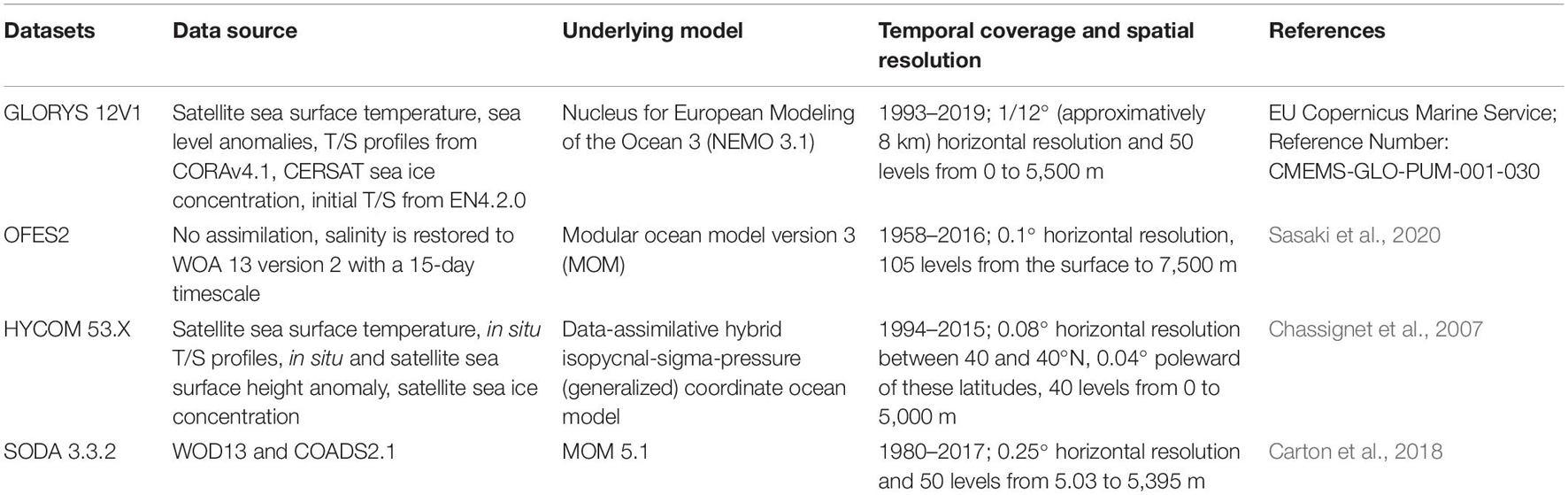
Table 1. Four model outputs used in this study for identifying the variability of the North Brazil Undercurrent (NBUC).
In situ Profiles
In this study, we use the analyzed in situ hydrographic profiles from EN4.2.1 (version 4 of the Met Office Hadley Centre EN) to explore the dependence of the NBUC on temperature and salinity. EN4.2.1 provides quality-controlled data profiles. The EN4.2.1 profiles include the World Ocean Database 2013 (details are given at https://www.metoffice.gov.uk/hadobs/en4/en4-0-2-data-sources.html), Argo profiling float (Argo, 2000),1,2 the Global Temperature and Salinity Profile Project (Sun et al., 2010), and others. All the profiles went through strict quality-controlled analysis (Good et al., 2013) and bias correction (Gouretski and Reseghetti, 2010). In this study, only the profiles marked as “good” in the quality-controlled flags are chosen for the NBUC-related analysis.
Method
Estimation of North Brazil Undercurrent Variability
This study explores the temporal variability of the NBUC from 11 to 5°S (from the origin to transition zones; Dossa et al., 2021). NBUC transport is defined as the meridional flow from the coast to the edge of the NBUC (Zhai et al., 2021) and from the surface to 1,200 m (Hummels et al., 2015). The edge of the NBUC is defined as the location where its meridional velocity is half of the maximum meridional velocity at the same zonal lines (Figure 2). In the three high-resolution models, the width between the edge and the coast is generally smaller than 1°, and SODA 3.3.2 shows a slightly larger width, 1–2°. The ensemble mean of the four model outputs is smaller than 1°. A slight change in the definition of the NBUC does not impact our results (see Supplementary Figures 1, 2). Hummels et al. (2015) defined the width of the NBUC (in their Figure 1) in the upper 300–400 m as 1.5° from the coast and 0.5–1° at 400–1,000 m by using alongshore velocity data from seven ship sections and moored observations. Dossa et al. (2021) did not show the width of the NBUC, but they showed that the core of the NBUC from GLORYS12V1 has shifted 15 km offshore relative to the observations from ship surveys. Nevertheless, the width of the NBUC from four model outputs in our analysis is generally consistent with the results from observations, with an acceptable difference.
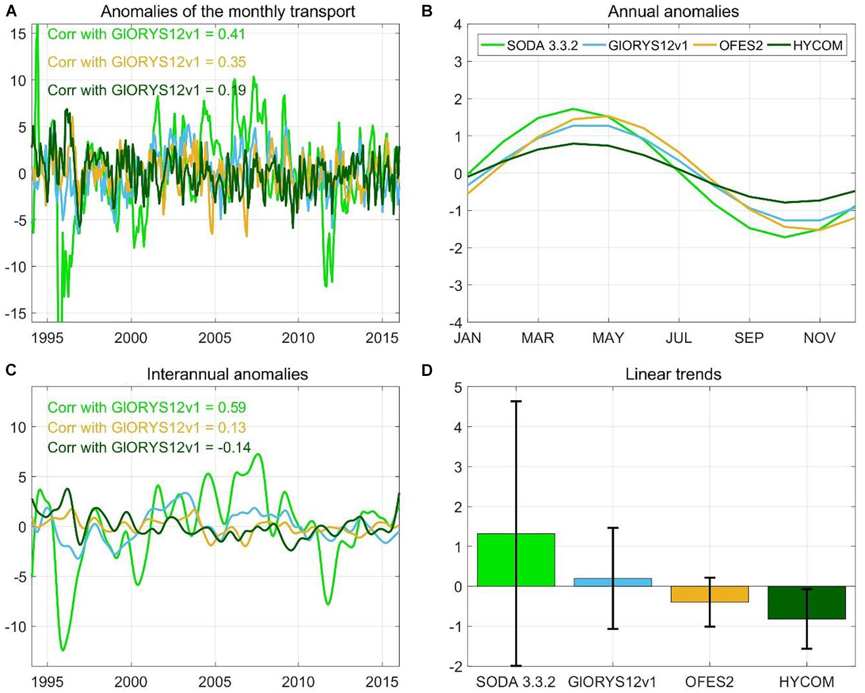
Figure 2. Comparison of North Brazil Undercurrent (NBUC) geostrophic transport variability (averaged between 5 and 11°S, with 1° interval) among four products during 1994–2015. (A) Time series of NBUC transport anomalies, (B) harmonic annual cycle, (C) interannual NBUC transport anomalies, and (D) slope of linear trends. The error bars in panel (D) indicate the 90% confidence level of the linear trend. The correlation coefficients between monthly and interannual NBUC geostrophic transport from GLORYS12V1 and other datasets are listed in panels (A,C). The units for the NBUC transport variability are Sv. The units for the slope of the linear trend are Sv/10 years.
The temporal variability in NBUC is divided into two components: annual (i.e., seasonal cycle) and interannual variations. The first step is to calculate the annual cycle of the NBUC based on annual harmonic least-square fitting. The annual cycle of NBUC transport is calculated as follows:
where V is the monthly NBUC transport, V0 is the climatological transport, A is the amplitude, and φ12 is the phase. Equation (1) is applied to the time series of the NBUC transport and is subtracted from the original time series. The remaining signal Vresidual is then filtered with a 12-month low-pass Hanning filter to derive the interannual time series of the NBUC transport.
Calculation of the Geostrophic Component of the North Brazil Undercurrent
The geostrophic components of the NBUC and ADCP-measured NBUC show similar magnitudes and spatial patterns (Stramma et al., 1995; Schott et al., 2005). In this study, the absolute geostrophic currents are calculated by referencing the meridional velocity at 2,000 m from each product. We have compared the absolute geostrophic NBUC transport with that directly derived from the meridional velocity and found that the two types of transport display similar variability on all time scales (not shown). The correlation coefficients between absolute geostrophic NBUC transport and the meridional velocity are 0.75–0.95 in the four model estimates, also indicating a strong similarity between the geostrophic velocities and meridional velocities (Supplementary Figure 3). Thus, it also implies that the contribution of Ekman drift and ageostrophy to NBUC transport variability is small compared to the geostrophic components in the upper 1,200 m. The geostrophic velocity is calculated based on this equation :
where v is the meridional component of the geostrophic velocity; ρ is the potential density; ρ0 is the reference density (1,027 kg/m3); x and z are the longitude and depth, respectively; g is gravity; and f is the Coriolis parameter. In this study, the velocity derived from Eq. (2) is defined as the density-based velocity.
We express the potential density using a linearized equation of state as:
where T is the conservative temperature, S is the absolute salinity, α is the thermal expansion coefficient, and β is the haline contraction coefficient. T0 and S0 are the constant temperature and salinity, respectively. It should be noted that T0 and S0 will be eliminated in the following calculation. Thus, the exact values are not our concern in this analysis. We combine Eq. (2) with Eq. (3) and write
where vT is the temperature-based geostrophic velocity, and vS is the salinity-based geostrophic velocity. Similar to Eq. (2), Eqs. (4 and 5) are integrated from 2,000 m, where the same velocity as used in density-based geostrophic velocity is given, to the upper layers to calculate vT and vS, respectively. The density-based, temperature-based and salinity-based geostrophic velocities are referenced on the same values (velocities at 2,000 m isobar from model outputs). A change in reference would influence the magnitude of the geostrophic variability, but it will not change the relations between the three types of the geostrophic velocities. We also calculated the correlation coefficients of the absolute geostrophic velocities using 1,200 and 2,000 m as references. The correlation coefficients of NBUC transport between 1,200 and 2,000 m is 0.96, 0.79, 0.98, and 0.83 for SODA 3.3.2, GLORYS12V1, OFES2, and HYCOM, respectively. This implies that a slight change in the reference level will not impact the results in this study.
To verify the robustness of temperature and salinity decomposition, we also sum the NBUC transport derived from vT and vS, and compare it with the density-based geostrophic NBUC transport (Supplementary Figure 3). The correlation coefficients of NBUC transport between the sum and density-based geostrophic transport in SODA 3.3.2, OFES2, and HYCOM are >0.75. GLORYS12V1 has a relatively small correlation coefficient, with a magnitude of 0.45. Possible reasons could include model configurations and methods of data assimilation. Further examination is out of the scope of this study. Nevertheless, all the correlations are significant. The decomposition works at least for SODA 3.3.2, OFES2, and HYCOM. Careful attention should be taken in GLORYS12V1 when interpreting NBUC transport between the sum of vT and vS, and the density-based geostrophic velocities.
Intercomparison of the North Brazil Undercurrent Variability Among Four Products
Generally, the monthly geostrophic NBUC transport varies substantially across datasets (Figure 2A). The correlation coefficients of monthly NBUC geostrophic transport between GLORYS12V1 and the other three datasets (Figure 2A) are generally small (<0.41). The correlation coefficient between GLORYS12V1 and HYCOM (a low-resolution model) is smaller than those between GLORYS12V1 and SODA 3.3.2, indicating that the resolution of the models does not play the major role in the largest difference among the inter-model comparison in this study.
However, the geostrophic NBUC transport based on different datasets agrees relatively well for the harmonic annual cycle (Figure 2B). The consistency between models implies that the underlying dynamics driving the annual cycle of NBUC transport are consistent among models. Transport is strongest during April-May and weakest during September-November. The results here agree with results from two surveys in spring 2015 and fall 2017, which show stronger transport during April-May 2015 than during September-October 2017 (Dossa et al., 2021). The results based on low-resolution models (Zhai et al., 2021) also show that the NBUC transport (2–10°S) reaches a maximum in May and a minimum in November-December, consistent with our results. The results from a moored array at 11°S from Schott et al. (2005) show that the minimum NBUC transport occurs in October-November, agreeing with our results. However, the maximum in NBUC transport occurs in July, which is different from other observations and our results. HYCOM shows the smallest amplitude of the annual cycle (defined as the standard deviation) among the four datasets (Figure 3), with a magnitude of 0.56 Sv. SODA 3.3.2 and OFES2 show amplitudes of approximately 1.1–1.2 Sv (Figure 3), which are slightly smaller than the amplitudes from Schott et al. (2005), who show an annual harmonic amplitude of 1.5 Sv over 2000–2004 at 11°S. Hummels et al. (2015) find that the standard deviation of the NBUC transport obtained from a moored array between July 2013 and May 2014 is 1.8 Sv at 11°S.
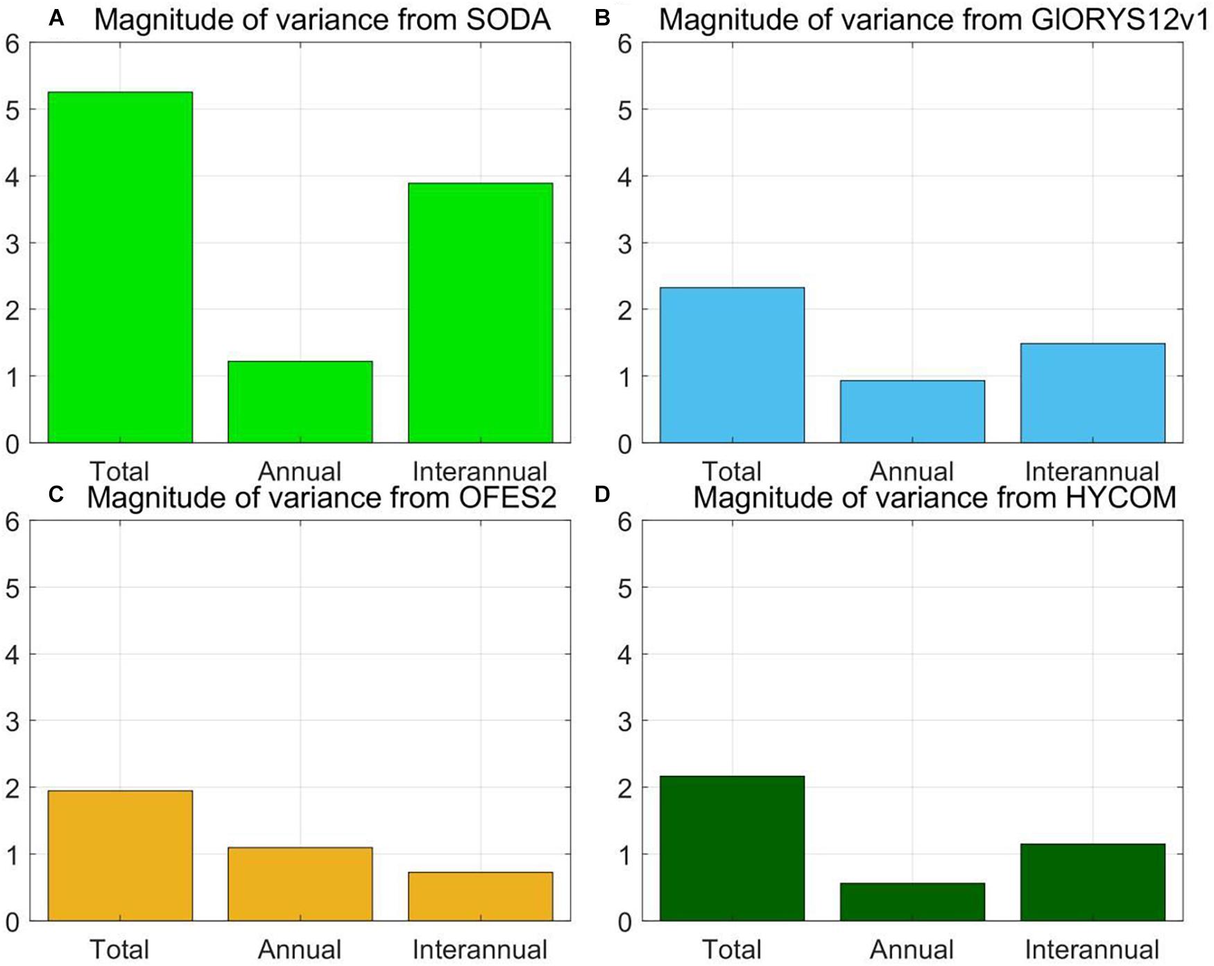
Figure 3. Magnitude of the North Brazil Undercurrent (NBUC) geostrophic transport variability on the different time scales in different products: (A) SODA 3.3.2; (B) GLORYS12V1; (C) OFES2; and (D) HYCOM. The magnitude of the NBUC variability is defined as one standard deviation of each time series on different time scales, including the original (marked as total), annual, and interannual scales. The units for all the bars are Sv.
On the interannual time scale (period > 12 months), the NBUC transport anomalies disagree substantially between datasets (Figure 2C). It is, in fact, hard to find any agreement among the different products on this time scale. Even though the correlations between GLORYS12v1 and the HYCOM and OFES2 are significant at the 90% confidence level, the correlation coefficients are relatively small, with values smaller than –0.14 to 0.13. The correlation between HYCOM and GLORYS12V1 is even negative. The correlation coefficient between SODA 3.3.2 and GLORYS12V1 is 0.59, which is relatively large compared to other coefficients. The higher correlation coefficients between SODA 3.3.2 and GLORYS12V1 than the others suggest that the model’s resolution is not a key component driving the difference in NBUC transport among models. However, we would like to emphasize that the low-resolution models (>0.5°) are incapable of resolving the NBUC width (∼0.5° at approximately 1,000 m from Hummels et al., 2015). The discrepancy between OFES2 and the other two high-resolution models (i.e., HYCOM and GLORYS12V1) could be because OFES2 is a hindcast output with no assimilation, while the other two models assimilate a large number of different types of observations (shown in Table 1). Large discrepancies among datasets can also be attributed to the treatment of observations and parameterization of the errors near the western boundaries (Mignac et al., 2018).
The maximum magnitude of interannual NBUC variability occurs in SODA 3.3.2, with a value of 3.89 Sv (Figure 3). The GLORYS12V1 and HYCOM show similar magnitudes of approximately 1.1–1.5 Sv. OFES2 has the smallest magnitude (0.72 Sv) among the four datasets. Estimates based on ship sections (ADCP sections) and a moored array suggest an amplitude of 1.2 Sv from 2000 to 2004 (Schott et al., 2005). Thus, the results from GLORYS12V1 and HYCOM are consistent with the observations.
From 1994 to 2015, NBUC transport derived from HYCOM shows a significant negative trend, with a value of –0.8 ± 0.7 Sv per 10 years. However, the other three datasets do not show any significant trends in the annual mean NBUC transport (Figure 2D). Whether the NBUC has been subject to a trend over the past years is currently under debate. Hummels et al. (2015) suggested that the NBUC does not have a significant trend by using moorings, ADCP sections (2000–2004, 2013–2014), and a high-resolution ocean model (1956–2007). However, Marcello et al. (2018) found a significant positive trend (1970–2015) in NBUC using a reanalysis data. It should be noted that discrepancies between the trends of NBUC transport could result from different analysis periods. Indeed, visual inspection of Marcello et al.’s (2018) Figure 9 does not indicate significant changes over the period 2000–2013. Thus, the two studies appear to agree on the absence of a trend for this period.
Salinity and Temperature Contributions to the North Brazil Undercurrent
On the long-term average, the absolute meridional geostrophic velocity derived from the individual model estimates (Figures 4A,D,G,J) is consistent with the ensemble mean meridional velocity (Figure 1). Northward velocities with a magnitude larger than 0.4 m/s are confined west of 34°W, while weaker southward flows are found to the east of 34°W. The NBUC velocity core (maximum in NBUC velocity) is found below 100 m in all datasets. These results are consistent with previous in-situ observations, which found cores in the upper 100 to 400 m (Stramma et al., 1995; Schott et al., 2005; Dossa et al., 2021).
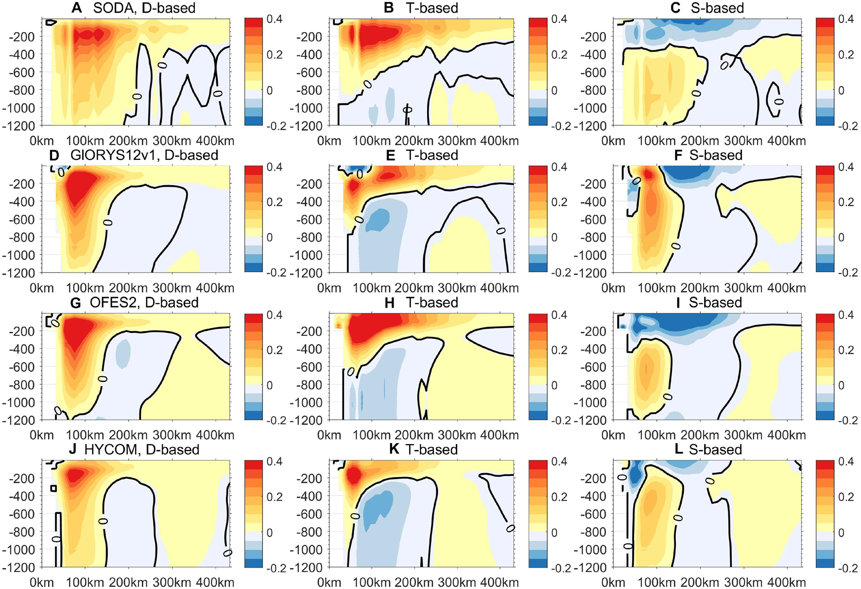
Figure 4. Absolute geostrophic meridional velocities derived from density (A,D,G,J), temperature (B,E,H,K), and salinity (C,F,I,L) in SODA 3.3.2 (A–C), GLORYS12V1 (D–F), OFES2 (G–I), and HYCOM (J–L). The velocities are derived from the average between 1994 and 2015 and from 5°S to 11°S. The x-axis is defined as the distance from the sea surface coast. The black contour is zero velocity. The units are m/s.
We use Eqs. (4 and 5) to estimate the contributions from temperature and salinity to the meridional geostrophic velocity. In the upper 1,200 m, both components are important to the density-based geostrophic velocity (Figure 4). The temperature-based velocity is generally dominant in the upper 400 m, while salinity-based velocity dominates below. High salinity waters formed in the subtropical gyre are being pushed to the western side (Liu and Qu, 2020), leading to saltier waters in the vicinity of the northeastern Brazilian coast and hence setting up a zonal salinity gradient. The negative zonal salinity gradient leads to a negative salinity-based velocity in the upper 400 m (Eq. 4; note that f < 0). At the same time, warmer waters (Stramma and England, 1999; Azar et al., 2020) are also found in the west as the SACW in the upper 400 m (this depth slightly varies between datasets), which corresponds to a positive vertical shear of the northward velocity (Eq. 3). As a result, the temperature-based velocity is opposite to the salinity-based velocity.
For the density-based meridional velocity below 400 m, the contribution of temperature-based and salinity-based velocities to the geostrophic velocity is reversed in all model outputs. The salinity-based velocity dominates the northward geostrophic velocity, and the temperature-based velocity is southward with a smaller magnitude. The zonal salinity gradient below 400 m is opposite to that in the upper layer. This is because fresh AAIW is generally transported to the Northern Hemisphere by the western boundary current (da Silveira et al., 1994; Schott et al., 2005; Fu et al., 2019). The near-coastal water at depth (AAIW located) is generally fresher than that away from the coast, leading to a negative salinity gradient and positive vertical shear.
The total variability of the meridional geostrophic velocity is calculated as one standard deviation of the monthly values from 1994 to 2015. The magnitudes in the density-based meridional geostrophic velocity variances from all model outputs are smaller than 0.2 m/s (Figure 5). Relatively larger variability is found between 35 and 34°W in the vicinity of the NBUC. The magnitude of variability of the temperature-based and salinity-based velocities shows a larger value than the density-based velocities in each model output. Furthermore, the magnitude of variability from the temperature-based and salinity-based velocities is generally larger than 0.2 m/s and shows similar spatial distributions (Figure 5). This suggests that the temperature and salinity contributions tend to cancel each other out.
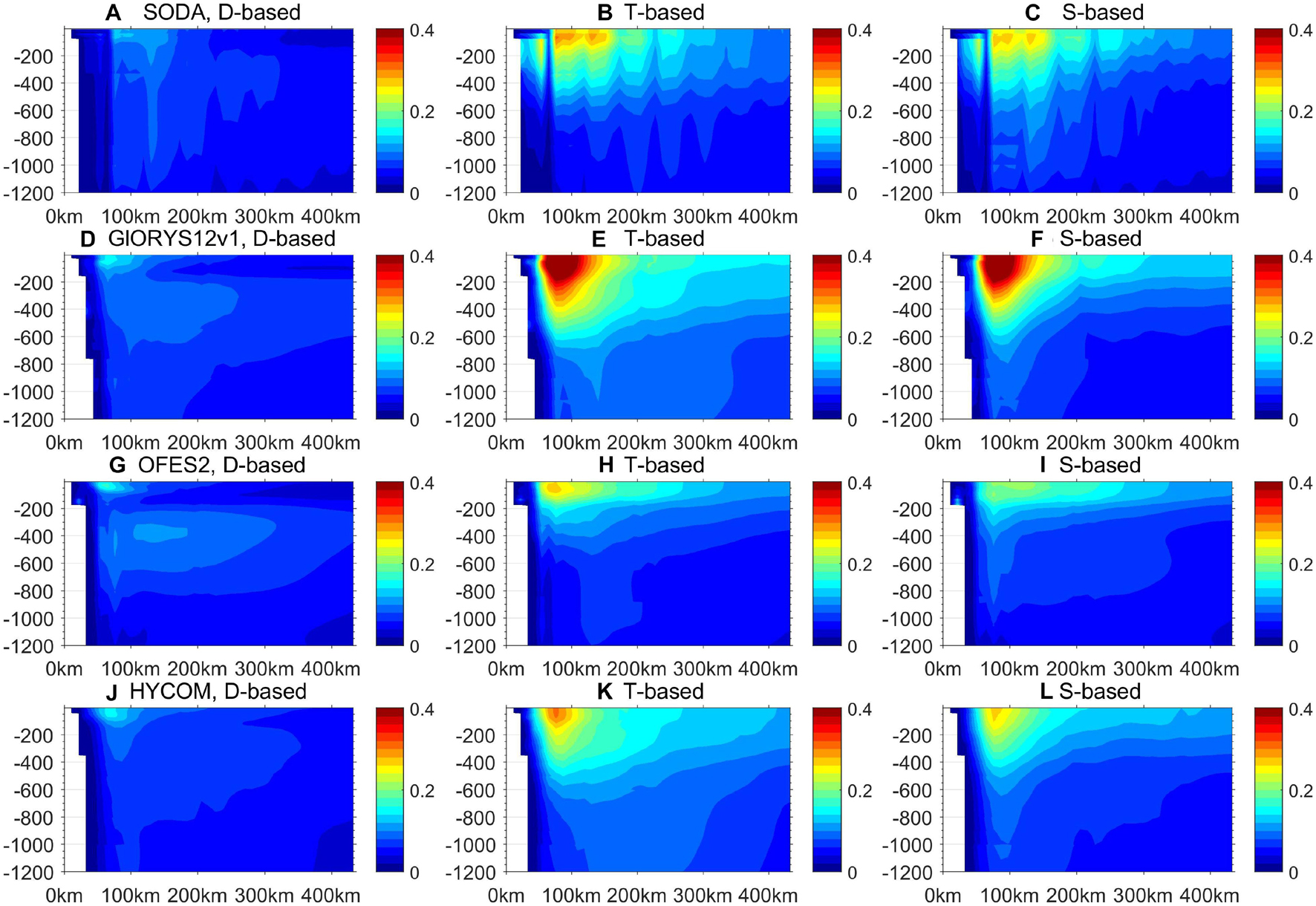
Figure 5. One standard deviation of the absolute geostrophic meridional velocity derived from density (A,D,G,J), temperature (B,E,H,K), and salinity (C,F,I,L) in SODA (A–C), GLORYS12V1 (D–F), OFES2 (G–I), and HYCOM (J–L). One standard deviation of the velocities is derived from monthly values from 1994 to 2015 and averaged between 5°S and 11°S. The x-axis is defined as the distance from the sea surface coast. The units for velocity are m/s.
To further explore the contribution of salinity and temperature to the variability of the meridional geostrophic velocity, temporal variability on different time scales is shown and quantified (Figures 6–8). On the annual time scale, the temperature-based and salinity-based velocity variances are larger than the density-based variance (Figure 6) in all models. Furthermore, the harmonic annual cycles of salinity-based and temperature-based velocity anomalies are 180° out of phase. From May to September, the temperature-based velocity shows positive anomalies, and the salinity-based velocity shows negative anomalies. The signs are reversed from October to the next March. The magnitude of the harmonic temperature-based variability is larger than that of salinity-based variability (or equal in results from HYCOM). The maximum/minimum density-based velocity anomalies have the same signs as the temperature-based velocity anomalies in SODA 3.3.2, OFES2, and HYCOM.
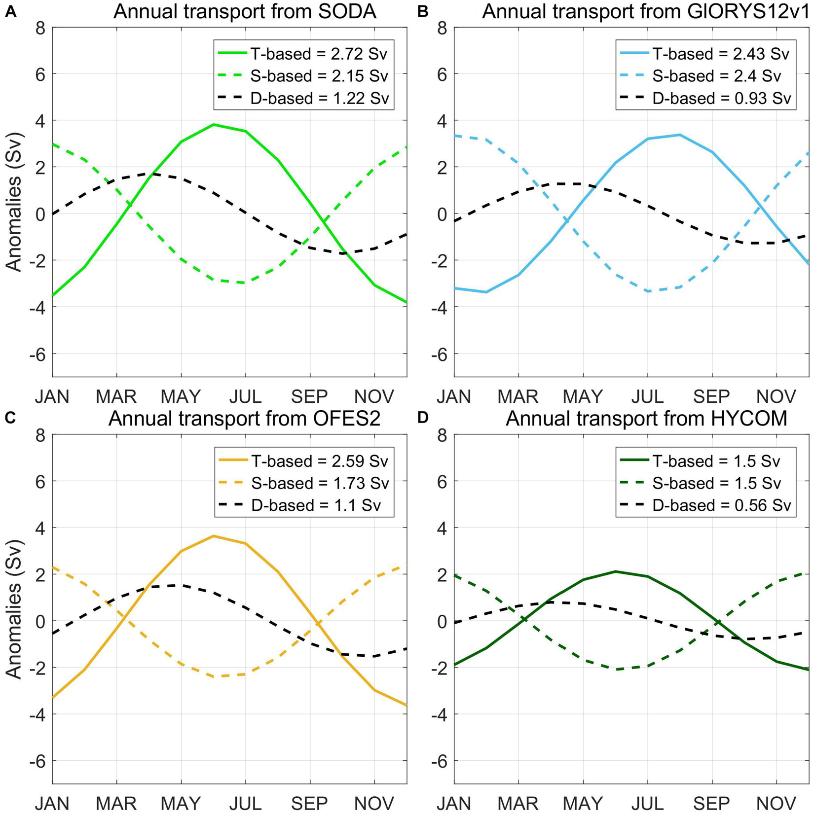
Figure 6. Time series of the annual North Brazil Undercurrent (NBUC) transport anomalies in different products: (A) SODA 3.3.2; (B) GLORYS12V1; (C) OFES2; and (D) HYCOM. The colored solid lines denote the temperature-based velocity, the colored dashed lines denote the salinity-based velocity, and the black dashed lines denote the density-based velocity. One standard deviation of each type of annual variability is listed in the legend. The unit of the annual NBUC transport anomalies is Sv.
On the interannual time scale, the temperature-based and salinity-based velocity variances show a similar relationship as those on the annual time scale (Figure 7). The temperature-based and salinity-based velocity anomalies generally show opposite signs and the magnitude of the variances of salinity/temperature-based velocities are larger than the density-based velocity variability in all datasets. To further assess the relation between temperature-based and salinity-based velocity anomalies, correlation coefficients are calculated. The two time series show significant (over 90% confidence level) anti-correlations in all models. The largest anti-correlation coefficients occur in GLORYS12V1 (–0.96), and the smallest anti-correlation coefficients occur in HYCOM (–0.77). In SODA 3.3.2, salinity-based variability is larger than the temperature-based variability, while in the other three model estimates, temperature-based velocity variability is larger.
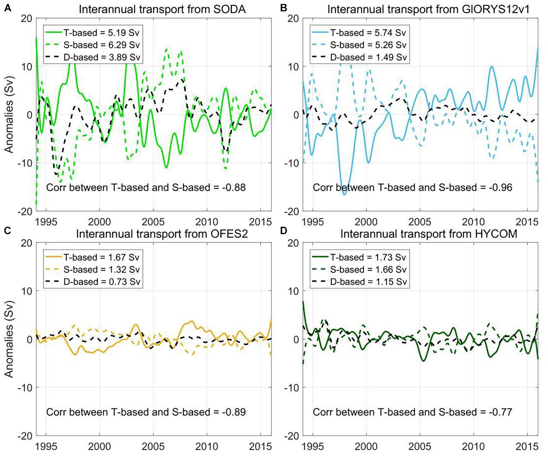
Figure 7. Time series of the interannual North Brazil Undercurrent (NBUC) transport anomalies in different products: (A) SODA 3.3.2; (B) GLORYS12V1; (C) OFES2; and (D) HYCOM. The colored solid lines denote the temperature-based velocity, the colored dashed lines denote the salinity-based velocity, and the black dashed lines denote the geostrophic velocity. One standard deviation of interannual variability is listed in the legend. The correlation coefficients between the temperature-based and salinity-based NBUC time series are listed in each figure. All the correlation coefficients satisfy the 90% confidence levels (not shown). The unit of the interannual NBUC transport anomalies is Sv.
For the linear trend of the annual mean NBUC transport from 1994 to 2015 (Figure 8), the temperature-based velocity shows opposite trends to the salinity-based velocity in SODA 3.3.2, GLORYS12V1, and OFES2. The linear trend of the density-based velocity is much smaller than those of the temperature-based and salinity-based velocities. However, in HYCOM, the temperature and salinity-based velocities both show a decreasing trend (not significant), leading to a larger decreasing trend in density-based velocity.
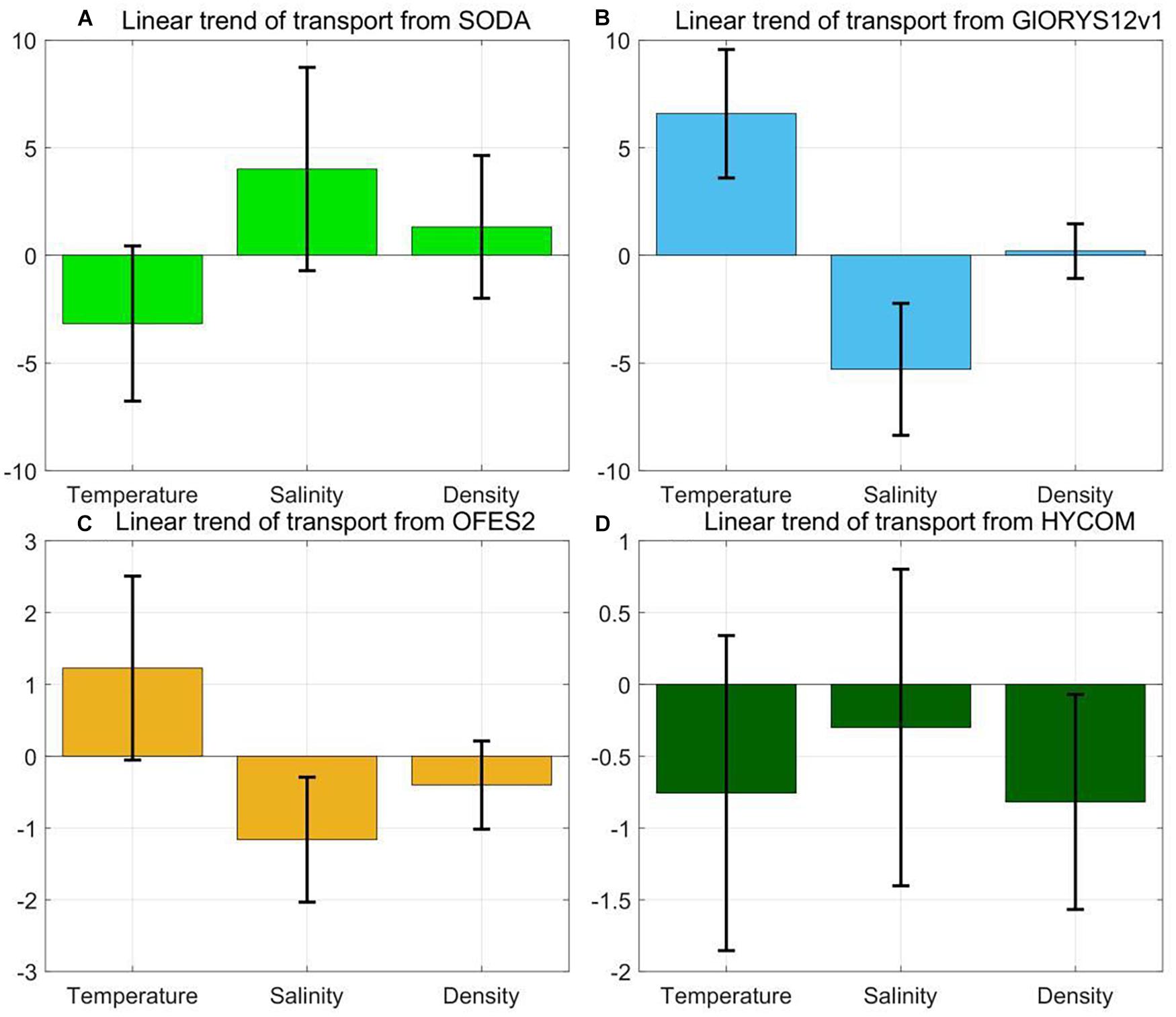
Figure 8. Linear trends of NBUC transport in (A) SODA 3.3.2, (B) GLORYS 12V1, (C) OFES2, and (D) HYCOM. The error bars indicate the 90% confidence level of the linear trend. The units for the slope of the linear trend are Sv/10 years.
In the previous section, we showed that the correlation coefficients of density-based NBUC geostrophic transport on the interannual time scales are small between models (magnitude < 0.37). Figure 9 shows the correlation coefficients of salinity-based and temperature-based NBUC transport between GLORYS12V1 and other models. The maximum correlation of temperature-based NBUC transport occurs in GLORYS12V1 and OFES2, with a magnitude of 0.49. The maximum in correlation coefficient of salinity-based NBUC transport also occurs in GLORYS12V1 and OFES2 3.3.2, with a magnitude of 0.42. However, correlations of temperature-based or salinity-based transport between GLORYS12V1 and the other two models are negative or insignificant. If correlation is calculated between HYCOM and OFES2 or SODA 3.3.2, smaller magnitudes (–0.2 to 0.35) of correlation coefficients for both the temperature-based and salinity-based transports. The negative or small correlation coefficients in temperature-based and salinity-based transport on the interannual time scale between models indicate large differences in salinity and temperature zonal gradients, which in turn explains the large discrepancy in the NBUC geostrophic transport between products.
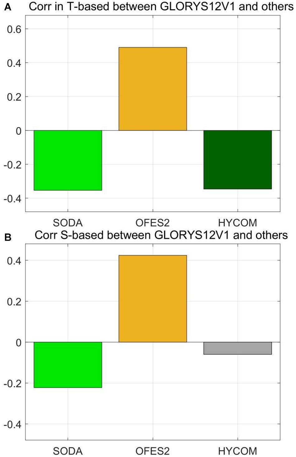
Figure 9. The correlation coefficients of (A) temperature-based and (B) salinity-based NBUC transport between GLORYS12V1 and SODA 3.3.2, HYOCM and OFES2. The gray bar indicates the correlation did not pass the 90% confidence level. The NBUC transports are averaged between 5°S and 11°S.
Discussion
The Temperature and Salinity Relation in Observation
Section “Salinity and Temperature Contribution to the North Brazil Undercurrent” shows that the temperature-based and salinity-based geostrophic NBUC transport variability tends to be compensated in all models. To verify the results, we have collected profiles from EN4 datasets, and assessed the relationship between temperature and salinity within the NBUC region using in situ data.
The number of in situ observations decreases with depth. To better make use of the available hydrographic profiles, we compare the zonal density gradients averaged from the sea surface to 1,200 m with those averaged to a smaller depth. We find that the density-based geostrophic NBUC transport integrated from the surface to 700 m is not very different from that averaged from the surface to 1,200 m (Figure 10), with temporal correlation coefficients higher than 0.9 in all models. Thus, we selected the temperature and salinity profiles from the EN4 database that are near the NBUC and cover at least 700 m. There are only about 20–40 profiles that match our criteria between 7 and 9°S near the western boundary (Figure 11). At 11°S, there are 100–120 profiles in the coastal regions.
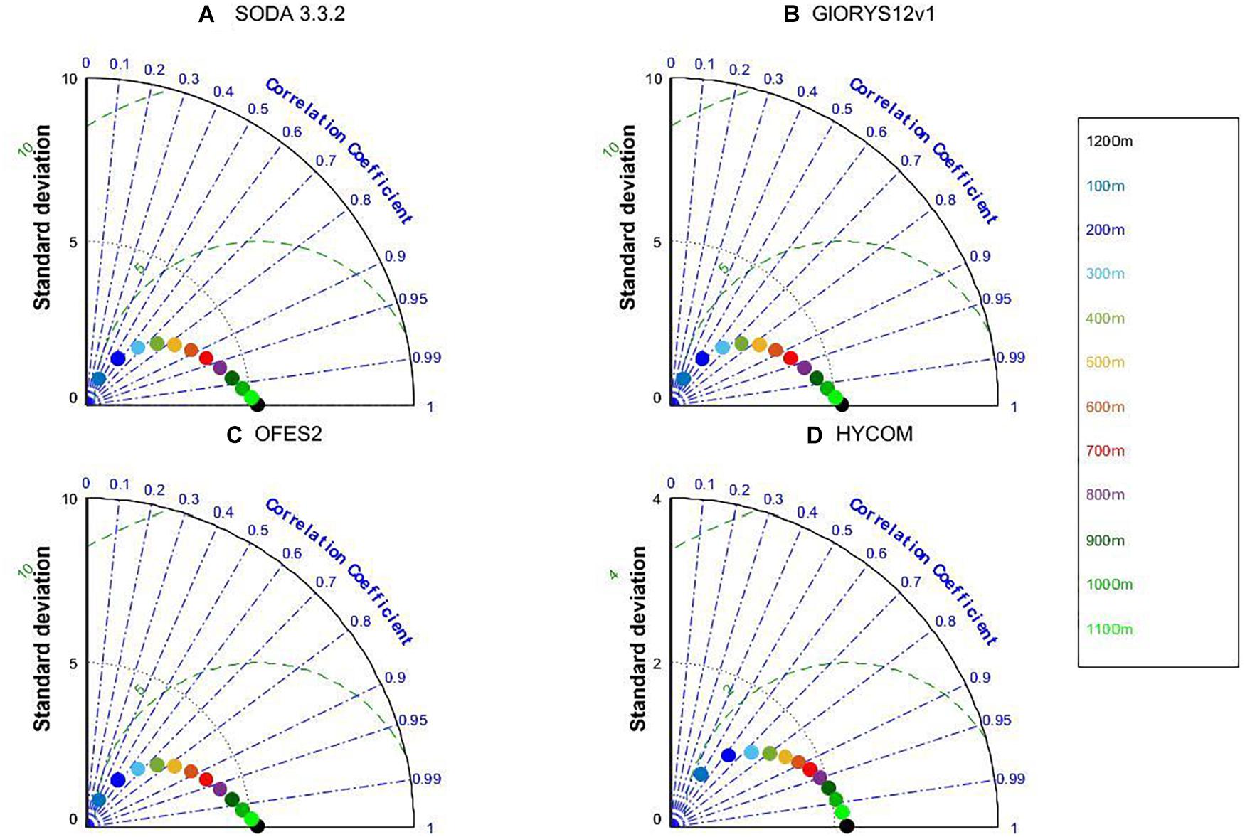
Figure 10. The Taylor diagram of density-based NBUC geostrophic transport derived from (A) SODA 3.3.2, (B) GLORYS 12V1, (C) OFES2, and (D) HYCOM. Different colors show that the lower limit for the integral of the NBUC transport at certain depths (100 m is blue and 1200 m is black). The units for standard deviation for the transport is Sv.
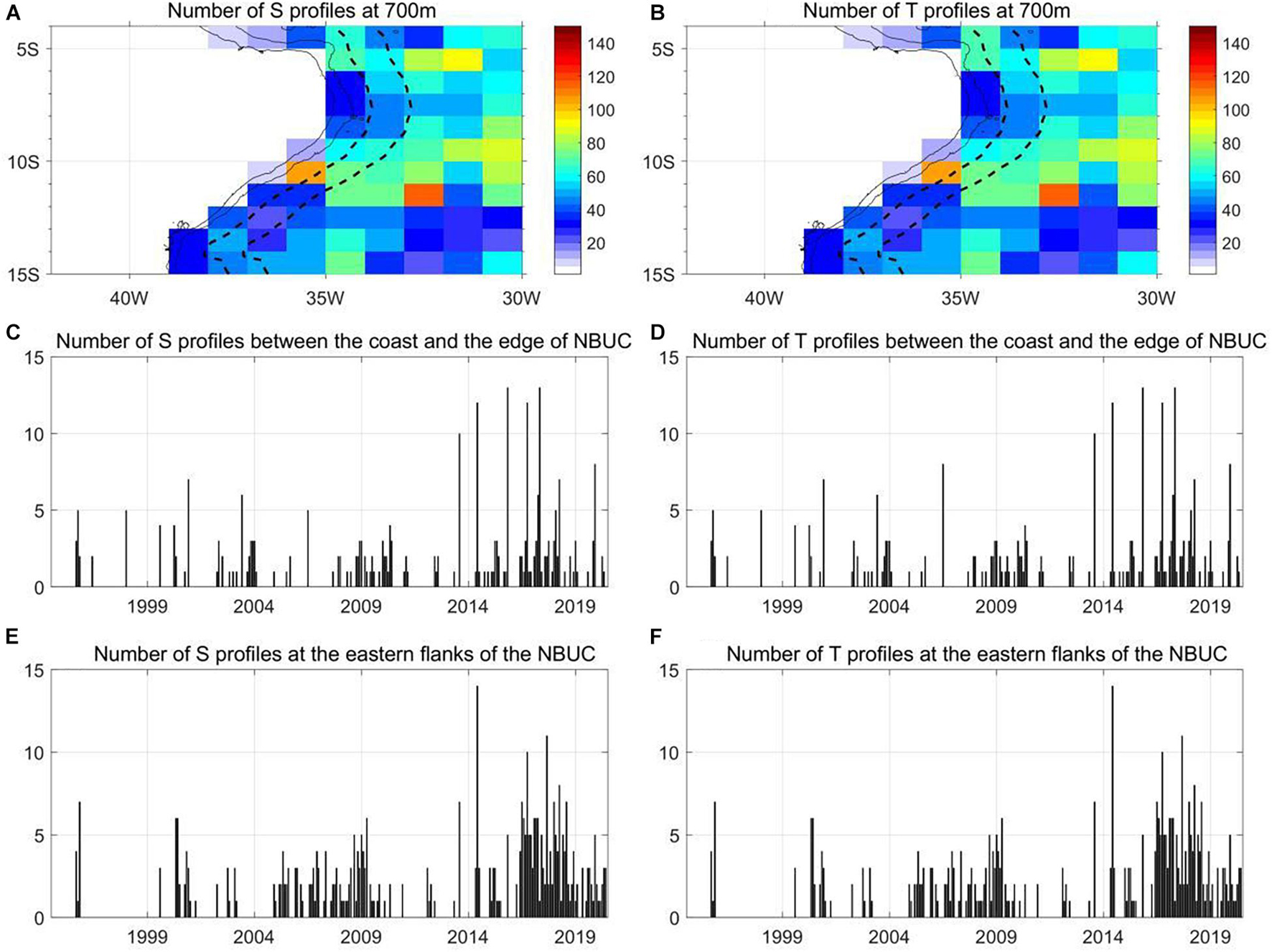
Figure 11. Spatial and temporal distribution of the number of (A,C,E) salinity and (B,D,F) temperature in situ profiles derived from EN4. The black solid lines in panels (A,B) denote the coastline and 1,000 isobars under the sea surface. The black dotted lines in panels (A,B) denote the edge of the NBUC and the eastern section of the NBUC (which is defined as 1° eastward away from the NBUC edge). Panels (C,D) denote the number of in situ salinity/temperature profiles located between the coast and the edge of the NBUC from 11 to 5°S. Panels (E,F) denote the number of in situ salinity/temperature profiles located between the edge of the NBUC and 1° away from the edge.
Profiles between the coast and the edge of the NBUC and those east of the NBUC are unevenly distributed. Observations mainly occur 2005–2009 and 2017–2020. At other times, observations are less frequent, which can explain why the interannual variability of the NBUC transport shows a large discrepancy between the models.
Based on in situ observations from EN4, we have calculated the geostrophic temperature-based and salinity-based geostrophic NBUC transport by assuming a reference level of no motion at 700 m (Figures 12, 13). We emphasize that the reference level should not influence the temperature and salinity relationship because the relationship mainly depends on the zonal salinity and temperature gradients which is discussed in the following section.
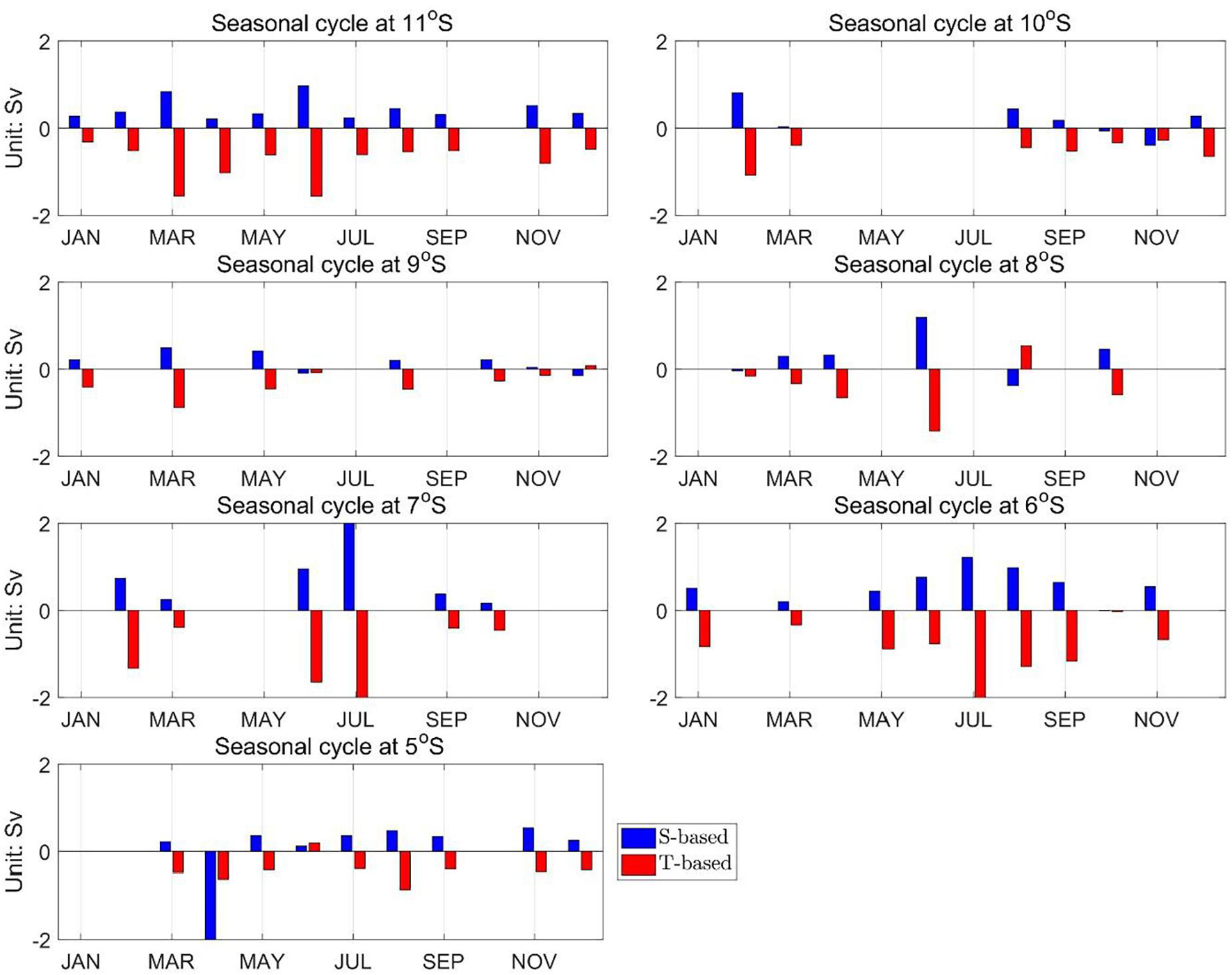
Figure 12. Seasonal cycle temperature/salinity-based geostrophic transport anomalies derived from in situ profiles at different latitudes within the North Brazil Undercurrent (NBUC) region from 1994 to 2020. The transports are calculated from the integral of geostrophic velocity from the sea surface to 700 m. The missing data is due to lack of observations. The units for the transports are Sv.
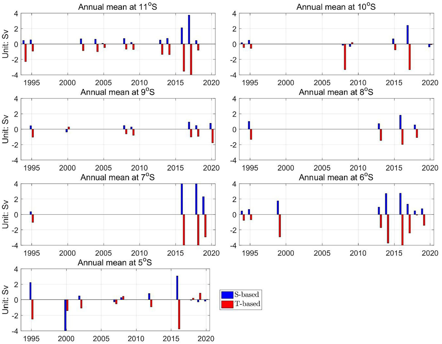
Figure 13. Interannual temperature/salinity-based geostrophic transport anomalies derived from in situ profiles at different latitudes within the North Brazil Undercurrent (NBUC) region from 1994 to 2020. The transports are calculated from the integral of geostrophic velocity from the sea surface to 700 m. The units for the transports are Sv.
From 11 to 5°S, the salinity-based and temperature-based geostrophic NBUC transport are opposite signed in most months of the annual cycle. At 11, 7, and 6°S, there is a 100% probability when the salinity-based and temperature-based geostrophic transports have opposite signs. At other latitudes, there is over 70% probability when the salinity-based and temperature-based signs are opposite. Thus, the results based on in situ profiles on the annual time scale are consistent with the results from models, and they show that the salinity and temperature gradients mostly compensate for each other.
From an interannual perspective, the number of temperature and salinity profiles is extremely low. For example, data cover 4 years out of 27 years (from 1994 to 2020) at 7 and 8°S. At 11°S, there are 12 years out of 27 years (from 1994 to 2020), which is the largest temporal coverage among the 5–11°S region. Thus, the estimation of the interannual variability in geostrophic transport is likely to be biased due to the lack of data. Nevertheless, based on the available data, we find that the salinity-based and temperature-based geostrophic NBUC transport is opposite signed 90% of the time from 11 to 5°S. Thus, the compensation between salinity- and temperature-based geostrophic transport still dominates, in agreement with the model results.
Possible Cause of the Relation Between Salinity-Based and Temperature-Based Geostrophic North Brazil Undercurrent Transport
To investigate the cause of the compensation of temperature-based and salinity-based NBUC geostrophic transport, we have calculated the 0–1,200 m averaged temperature and salinity zonal gradient within the NBUC region on annual, interannual time scales, and linear trends in all models. Results show that the temperature and salinity zonal gradients also tend to be compensated on those time scales (Supplementary Figures 4–6), consistent with the temperature and salinity relations in geostrophic NBUC transport (Figures 7, 9, 10). Saltier (warmer) waters occur near the coast in the upper 200 m than that 100–200 km away from the coast (Figures 1D,F). Below 200 m, fresher (cold) waters are located near the coast than those 50–100 km away from the coast. Thus, zonal salinity and temperature gradient are compensated which is probably associated with the spatial distribution of unique water masses within the NBUC. In the upper 200 m, STUW occurs below the mixed layer. Temperature and salinity within the STUW have a compensatory relationship during its equatorial transport in the North Atlantic (Qu et al., 2016). We suspect the same mechanism would also apply in the South Atlantic STUW within the NBUC. At approximately 300–500 m, the compensated temperature and salinity anomalies within the SACW (=26.3 kg/m3) are reported to be transported from Agulhas leakage to the western South Atlantic ocean (Kolodziejczyk et al., 2014, results are based on Argo). Thus, temperature and salinity compensation are suspected to exist in those layers. The origins and causes of the compensated temperature and salinity relation (on different time scales) within the NBUC region are out of the scope of this analysis, and they should demand more thorough investigation in the future.
The Implication for Large Discrepancies in North Brazil Undercurrent Among Models and the T-S Relationship
Large discrepancies in NBUC transport among datasets are expected for low-resolution model outputs or reanalysis data but not for high-resolution model outputs. The NBUC is a narrow western boundary current. If the horizontal resolution is sparser than 0.5° (i.e., the width of the NBUC at the subsurface layers), it will generally be impossible for these models to represent the real NBUC. However, in high-resolution model outputs (resolutions ≤ 0.25°), the large discrepancy among datasets indicates that the mechanism driving the NBUC low-frequency variability is still unknown. We are unable to determine the real NBUC transport variability or trend, which also prevents us from identifying/exploring the role of NBUC in the AMOC. STC and AMOC have a profound impact on the Atlantic and global climate. A better understanding of the global climate demands improvement in the simulation of the NBUC. Future work is needed to investigate the causes of the discrepancy among models and the mechanism driving the NBUC variability.
In this study, we also show that the discrepancy in NBUC transport among models can be attributed to the difference in zonal temperature and salinity gradients. Furthermore, the temperature and salinity-based geostrophic transport show a compensatory relation. The results have two implications:
(1) This study shows that temperature-based geostrophic velocities deeper than 600 m isobar have an opposite sign with meridional velocity in NBUC from a climatological perspective, but in the upper 600 m, temperature-based geostrophic velocities and meridional velocity have the same sign. It could serve as the first step in understanding the role of the temperature on the NBUC, and it will be beneficial for identifying the processes associated with meridional heat fluxes across the equator.
(2) This study shows that salinity-based NBUC transport variability usually has the same order of magnitude as those from temperature-based variability (Figures 6, 7). Thus, salinity observations are important for representing NBUC variability. The role of the salinity on the NBUC will be a foundation of understanding how the salinity and velocity fields are coupled, which could assist the improvement of the model simulation.
Conclusion
In this study, we have analyzed the trend and the variability of the NBUC transports on the annual, and interannual time scales over the 1994–2015 period. By comparing the NBUC transport from three high-resolution (≤1/10°) models and one low-resolution (=0.25°) model, we find large differences in NBUC interannual variability and linear trends. Decomposing the absolute geostrophic velocity into salinity and temperature contributions, we find the following:
(1) Large differences between models occur in geostrophic NBUC transport on the interannual time scale and trend from 1994–2015.
(2) The salinity-based and temperature-based transport anomalies tend to be opposite-signed on all time scales. Thus, variability in the temperature and salinity-based geostrophic transport (and their zonal gradients) partially cancels each other out in the NBUC among model outputs.
The discrepancy in NBUC variability and trend among models in this study could be attributed to the parameterization of eddies or other variables or assimilation method (Mignac et al., 2018). The exact causes in the model discrepancy are out of the scope of this analysis. Further analysis is under way to pin out the cause of the discrepancy.
The compensated salinity/temperature-based geostrophic anomalies lead to a smaller magnitude of the density-based geostrophic transport variance. Thus, to reduce the discrepancy in NBUC transport variability among datasets, one must have reliable temperature and salinity profiles long enough for variability analysis. From 1994 to 2020, the number of in situ profiles in the vicinity of the NBUC region was relatively low. Thus, many questions regarding the variability of the NBUC on other time scales remain open. This demands sufficient salinity and temperature observations to derive the variability of the NBUC, which is even lacking in the Argo era (because Argo profiles near the coast are rare).
One aspect not shown in this study is the origins of the salinity and temperature compensation. Where temperature and salinity anomalies come from and how they transport will be vital in understanding the causes of NBUC variability. This study calls for a full investigation of the origins of the temperature and salinity variability.
Data Availability Statement
GLORYS12V1 for this study can be found at the EU Copernicus Marine Service (https://resources.marine.copernicus.eu/?option=com_csw&view=details&product_id=GLOBAL_REANALYSIS_PHY_001_030). OFES2 can be found at the Japan Agency for Marine-Earth Science and Technology (https://doi.org/10.17596/0002029). HYCOM can be found at the National Ocean Partnership Program (https://www.hycom.org/data/glbv0pt08/expt-53ptx). SODA 3.3.2 can be found at the College of the Computer Mathematical and Natural Sciences, Department of Atmospheric and Oceanic Science, University of Maryland (https://www2.atmos.umd.edu/%7Eocean/index_files/soda3_readme.htm). EN4 profiles are from the Met Office Hadley Centre (https://www.metoffice.gov.uk/hadobs/en4/en4-0-2-data-sources.html). Argo profiles from EN4 were collected and made freely available by the International Argo Program and the national programs that contribute to it (https://argo.ucsd.edu, https://www.ocean-ops.org, and https://doi.org/10.17882/42182). The Argo Program is part of the Global Ocean Observing System.
Author Contributions
HL and ZW conceived and led the manuscript. HL wrote the manuscript. IR, XN, and CL provided the input and/or edited the text. All authors contributed to the article and approved the submitted version.
Funding
This research was funded by the National Natural Science Foundation of China (42006005 and 41821004), the Postdoctoral Innovation Research Program of Shandong Province (SDSBSH202002), the Qingdao Postdoctoral Applied Research Project (QDBSH202004), and the China Ocean Mineral Resources R&D Association (DY135-S2-2).
Conflict of Interest
The authors declare that the research was conducted in the absence of any commercial or financial relationships that could be construed as a potential conflict of interest.
Publisher’s Note
All claims expressed in this article are solely those of the authors and do not necessarily represent those of their affiliated organizations, or those of the publisher, the editors and the reviewers. Any product that may be evaluated in this article, or claim that may be made by its manufacturer, is not guaranteed or endorsed by the publisher.
Acknowledgments
We gratefully acknowledge the efforts of all parties involved in collecting data. We thank Shan Gao from the Institute of Oceanology, Chinese Academy of Sciences for collecting the data. We also thank Ryo Furue from JAMSTEC for his valuable and instructive inputs and editing on the manuscript. We also thank Tengfei Xu from the First Institute of Oceanography for his input on the manuscript.
Supplementary Material
The Supplementary Material for this article can be found online at: https://www.frontiersin.org/articles/10.3389/fmars.2021.744833/full#supplementary-material
Footnotes
References
Araujo, M., Limongi, C., Servain, J., Silva, M., Leite, F., Veleda, D., et al. (2011). Salinity-induced mixed and barrier layers in the Southwestern tropical Atlantic Ocean off the Northeast of Brazil. Ocean Sci. 7, 63–73. doi: 10.5194/os-7-63-2011
Argo (2000). Argo Float Data and Metadata from Global Data Assembly Centre (Argo GDAC). SEANOE. doi: 10.17882/42182
Azar, E., Piango, A., Wallner-Kersanach, M., and Kerr, R. (2020). Source waters contribution to the tropical Atlantic central layer: new insights on the Indo-Atlantic exchanges. Deep Sea Res. Part I Oceanogr. Res. Pap. 168:103450. doi: 10.1016/j.dsr.2020.103450
Cabré, A., Pelegrí, J., and Vallès-Casanova, I. (2019). Subtropical-tropical transfer in the South Atlantic Ocean. J. Geophys. Res. Oceans 124, 4820–4837. doi: 10.1029/2019jc015160
Carton, J. A., Chepurin, G. A., and Chen, L. (2018). SODA3: a new ocean climate reanalysis. J. Clim. 31, 6967–6983. doi: 10.1175/JCLI-D-18-0149.1
Chassignet, E. P., Hulburt, H. E., Smedstad, O. M., Halliwell, G. R., and Hogan, P. J. (2007). The HYCOM (HYbrid Coordinate Ocean Model) data assimilative system. J. Mar. Syst. 65, 60–83. doi: 10.1016/j.jmarsys.2005.09.016
da Silveira, I. C., de Miranda, L. B., and Brown, W. S. (1994). On the origins of the North Brazil. Curr. J. Geophys. Res. Oceans 99, 22501–22512. doi: 10.1029/94JC01776
Daniel, V., Piola, A. R., Meinen, C. S., and Campos, E. J. D. (2018). Strong mixing and recirculation in the Northwestern Argentine Basin. J. Geophys. Res. Oceans 123, 4624–4648. doi: 10.1029/2018JC013907
Dossa, A. N., Silva, A. C., Chaigneau, A., Eldin, G., and Bertrand, A. (2021). Near-surface western boundary circulation off Northeast Brazil. Prog. Oceanogr. 190:102475. doi: 10.1016/j.pocean.2020.102475
Fu, Y., Wang, C., Brandt, P., and Greatbatch, R. J. (2019). Interannual variability of antarctic intermediate water in the Tropical North Atlantic. J. Geophys. Res. Oceans 124, 4044–4057. doi: 10.1029/2018JC014878
Garzoli, S. L., and Matano, R. (2011). The South Atlantic and the Atlantic meridional overturning circulation. Deep Sea Res. II 58, 1837–1847.
Good, S. A., Martin, M. J., and Rayner, N. A. (2013). EN4: quality controlled ocean temperature and salinity profiles and monthly objective analyses with uncertainty estimates. J. Geophys. Res. Oceans 118, 6704–6716. doi: 10.1002/2013jc009067
Gouretski, V., and Reseghetti, F. (2010). On depth and temperature biases in bathythermograph data: development of a new correction scheme based on analysis of a global ocean database. Deep Sea Res. Part I Oceanogr. Res. Pap. 57, 812–833. doi: 10.1016/j.dsr.2010.03.011
Hummels, R., Brandt, P., Dengler, M., Fischer, J., Araujo, M., Veleda, D., et al. (2015). Interannual to decadal changes in the western boundary circulation in the Atlantic at 11°S. Geophys. Res. Lett. 42, 7615–7622. doi: 10.1002/2015GL065254
Kolodziejczyk, N., Reverdin, G., Gaillard, F., and Lazar, A. (2014). Low-frequency thermohaline variability in the Subtropical South Atlantic pycnocline during 2002–2013. Geophys. Res. Lett. 41, 6468–6475. doi: 10.1002/2014gl061160
Larqué, L., Maamaatuaiahutapu, K., and Garçon, V. (1997). On the intermediate and deep water flows in the South Atlantic Ocean. J. Geophys. Res. Oceans 102, 12425–12440. doi: 10.1029/97JC00629
Liu, H., Li, S., and Wei, Z. (2021). Interannual variability in the subduction of the South Atlantic subtropical underwater. Clim Dyn 57, 1061–1077. doi: 10.1007/s00382-021-05758-0
Liu, H., and Qu, T. (2020). Production and fate of the South Atlantic subtropical underwater. J. Geophys. Res. Oceans 125:e2020JC016309. doi: 10.1029/2020JC016309
Marcello, F., Wainer, I., and Rodrigues, R. (2018). South Atlantic Subtropical gyre late 20th century changes. J. Geophys. Res. Oceans 123, 5194–5209. doi: 10.1029/2018JC013815
Mccarthy, G. D., Smeed, D. A., Johns, W. E., Frajka-Williams, E., Moat, B. I., Rayner, D., et al. (2015). Measuring the Atlantic meridional overturning circulation at 26°N. Prog. Oceanogr. 130, 91–111. doi: 10.1016/j.pocean.2014.10.006
Mignac, D., Ferreira, D., and Haines, K. (2018). South Atlantic meridional transports from NEMO-based simulations and reanalyses. Ocean Sci. 14, 53–68. doi: 10.5194/os-14-53-2018
Qu, T., Zhang, L., and Schneider, N. (2016). North Atlantic subtropical underwater and its year-to-year variability in annual subduction rate during the argo period. J. Phys. Oceanogr. 46, 1901–1916. doi: 10.1175/jpo-d-15-0246.1
Rabe, B., Schott, F. A., and Köhl, A. (2008). Mean circulation and variability of the tropical Atlantic during 1952–2001 in the GECCO assimilation fields. J. Phys. Oceanogr. 38, 177–192. doi: 10.1175/2007jpo3541.1
Reid, J. L. (1989). On the total geostrophic circulation of the South Atlantic Ocean: flow patterns, tracers, and transports. Progress In Oceanography 23, 149–244. doi: 10.1016/0079-6611(89)90001-3
Rodrigues, R. R., Rothstein, L. M., and Wimbush, M. (2007). Seasonal variability of the South Equatorial Current bifurcation in the Atlantic Ocean: a numerical study. J. Phys. Oceanogr. 37, 16–30. doi: 10.1175/jpo2983.1
Rühs, S., Getzlaff, K., Durgadoo, J. V., Biastoch, A., and Böning, C. W. (2015). On the suitability of North Brazil Current transport estimates for monitoring basin-scale AMOC changes. Geophys. Res. Lett. 42, 8072–8080. doi: 10.1002/2015GL065695
Sasaki, H., Kida, S., Furue, R., Aiki, H., and Taguchi, B. (2020). A Global Eddying Hindcast Ocean Simulation with OFES2. doi: 10.5194/gmd-2019-351
Schott, F. A., Brandt, P., Hamann, M., Fischer, J., and Stramma, L. (2002). On the boundary flow off Brazil at 5–10°S and its connection to the interior tropical Atlantic. Geophys. Res. Lett. 29:1840. doi: 10.1029/2002GL014786
Schott, F. A., Dengler, M., Zantopp, R., Stramma, L., Fischer, J., and Brandt, P. (2005). The shallow and deep western boundary circulation of the south atlantic at 5°-11°S. J. Phys. Oceanogr. 35, 2031–2053. doi: 10.1175/JPO2813.1
Silva, A. C., Bourles, B., and Araujo, M. (2009). Circulation of the thermocline salinity maximum waters off the Northern Brazil as inferred from in situ measurements and numerical results. Ann. Geophys. 27, 1861–1873. doi: 10.5194/angeo-27-1861-2009
Souza, A. D., Kerr, R., and Azevedo, J. D. (2018). On the influence of subtropical mode water on the South Atlantic Ocean. J. Mar. Syst. 185, 13–24. doi: 10.1016/j.jmarsys.2018.04.006
Stramma, L., and England, M. (1999). On the water masses and mean circulation of the South Atlantic Ocean. J. Geophys. Res. 1042, 20863–20884. doi: 10.1029/1999JC900139
Stramma, L., Fischer, J., and Reppin, J. (1995). The North Brazil Undercurrent. Deep Sea Res. Part I Oceanogr. Res. Pap. 42, 773–795. doi: 10.1016/0967-0637(95)00014-W
Sun, C., Thresher, A., Keeley, R., Hall, N., Hamilton, M., Chinn, P., et al. (2010). “The data management system for the global temperature and salinity profile programme,” in Proceedings of the OceanObs.09: Sustained Ocean Observations and Information for Society. Venice, Italy, 21-25 September 2009, Vol. 2, eds J. Hall, D. E. Harrison, and D. Stammer (ESA Publication WPP-306). doi: 10.5270/OceanObs09.cwp.86
Tuchen, F. P., Lübbecke, J., Brandt, P., and Yao, F. (2020). Observed transport variability of the Atlantic Subtropical Cells and their connection to tropical sea surface temperature variability. J. Geophys. Res. Oceans 125:e2020JC016592. doi: 10.1029/2020JC016592
Tuchen, F. P., Lübbecke, J., Schmidtko, S., Hummels, R., and Bning, C. W. (2019). The Atlantic subtropical cells inferred from observations. J. Geophys. Res. Oceans 124, 7591–7605. doi: 10.1029/2019jc015396
White, R. H. (2015). Using multiple passive tracers to identify the importance of the North Brazil undercurrent for Atlantic cold tongue variability. Q. J. R. Meteorol. Soc. 141, 2505–2517. doi: 10.1002/qj.2536
Zhai, Y., Yang, J., and Wan, X. (2021). Cross-equatorial anti-symmetry in the seasonal transport of the Western Boundary Current in the Atlantic Ocean. J. Geophys. Res. Oceans 126:e2021JC017184. doi: 10.1029/2021JC017184
Zhang, D., McPhaden, M. J., and Johns, W. E. (2003). Observational evidence for flow between the subtropical and tropical Atlantic: the Atlantic subtropical cells∗. J. Phys. Oceanogr. 33, 1783–1797.
Keywords: North Brazil Undercurrent, salinity-based geostrophic velocity, temperature-based geostrophic velocity, temporal variability, HYCOM, OFES2, GLORYS12V1
Citation: Liu H, Wei Z, Richter I, Nie X and Li C (2021) Influence of Salinity and Temperature Gradients on the Variability of the North Brazil Undercurrent. Front. Mar. Sci. 8:744833. doi: 10.3389/fmars.2021.744833
Received: 21 July 2021; Accepted: 01 September 2021;
Published: 20 September 2021.
Edited by:
Regina R. Rodrigues, Federal University of Santa Catarina, BrazilReviewed by:
Franz Philip Tuchen, GEOMAR Helmholtz Center for Ocean Research Kiel, GermanyShijian Hu, Institute of Oceanology, Chinese Academy of Sciences (CAS), China
Copyright © 2021 Liu, Wei, Richter, Nie and Li. This is an open-access article distributed under the terms of the Creative Commons Attribution License (CC BY). The use, distribution or reproduction in other forums is permitted, provided the original author(s) and the copyright owner(s) are credited and that the original publication in this journal is cited, in accordance with accepted academic practice. No use, distribution or reproduction is permitted which does not comply with these terms.
*Correspondence: Zexun Wei, d2VpenhAZmlvLm9yZy5jbg==