Comparing Uncertainty Associated With 1-, 2-, and 3D Aerial Photogrammetry-Based Body Condition Measurements of Baleen Whales

Introduction

An animal’s body condition is a crucial and indicative measure of its fitness, as it reflects the balance between energy intake and energetic investment in growth, maintenance, and reproduction (Jakob et al., 1996; Schulte-Hostedde et al., 2001). Body condition is defined as the energy stored in the body, which is assumed to reflect individual health, and can be expressed as any morphological, physiological, or biochemical measure of an individual’s energy reserves, independent of its structural size (Green, 2001; Peig and Green, 2009). As such, body condition reflects an individual’s foraging success and provides information on habitat quality and reproductive output (Stevenson and Woods, 2006). For example, in high quality habitats with increased availability of salmon, female North American brown bears (Ursus arctos) were in better body condition, produced larger litter sizes, and lived at greater population densities compared to females in lower quality habitats (Hilderbrand et al., 1999). As global temperatures rise, with consequences at local scales (Sippel et al., 2020), it is important to monitor the body condition of populations in rapidly changing habitats to inform conservation and management decisions, especially for marine species which may be disproportionally susceptible to changes in habitat (Lenoir et al., 2020).

Baleen whales can serve as “ecosystem sentinels,” as their body condition not only reflects the health of their populations, but the state of marine ecosystems (Moore, 2008; Bengtson Nash et al., 2018). As such, measurements of the body condition of baleen whales can help track their responses to environmental change and anthropogenic stressors. Aerial photogrammetry is a non-invasive method for acquiring morphological measurements of an individual’s energy reserves and provides an opportunity for assessing the body condition of cetaceans that are too large for capture and handling (Whitehead and Payne, 1978; Perryman and Lynn, 2002; Miller et al., 2012). Recently, unoccupied aircraft systems (UAS or drones) have greatly increased the capacity to obtain body condition measurements from aerial imagery to monitor baleen whale populations, especially in their role as ecosystem sentinels (Johnston, 2019; Castrillon and Bengtson Nash, 2020). These platforms are safer, yield higher resolution data, and are more accurate, immediate, and affordable compared to using traditional camera systems mounted on airplanes. Several studies have used UAS to measure body condition of baleen whales, including blue (Balaenoptera musculus), gray (Eschrichtius robustus), humpback (Megaptera novaeangliae), and Southern (Eubalaena australis) and North Atlantic (Eubalaena glacialis) right whales (Christiansen et al., 2016, 2018, 2020a,b, 2021; Durban et al., 2016; Lemos et al., 2020; Aoki et al., 2021). These studies have derived estimates of intra- and inter-seasonal variation across individuals and populations (Christiansen et al., 2016; Durban et al., 2016; Lemos et al., 2020), documented how calf growth rate is directly related to maternal loss during lactation (Christiansen et al., 2018), and even estimated body mass (Christiansen et al., 2019). However, several different photogrammetry-based methods for measuring body condition have emerged from these studies and, as Castrillon and Bengtson Nash (2020) argue, a standardization of measurements across studies is needed and uncertainty should be both quantified and minimized, as a measurement result is complete only when accompanied by a quantitative statement of its uncertainty (Taylor and Kuyatt, 1994).

Analyzing body condition in cetaceans using morphometric measurements made from aerial-photogrammetry typically relies on estimates in 1−, 2−, or 3-dimensions – a single width (SW), a projected dorsal surface area (SA), or a body volume (BV) measure, respectively (Figure 1). These 1−, 2−, or 3-dimensional (hereafter referred as 1D, 2D, and 3D, respectively) measurements are then converted into body condition indices – either using a ratio to correct for total length (TL) or using the residuals from a linear regression with TL – to provide a relative measure of an individual’s body condition in relation to its structural size and allow comparison among individuals and populations (Stevenson and Woods, 2006; Wilder et al., 2016). However, it is unknown how photogrammetric uncertainty scales across these 1D, 2D, and 3D measurements, or how this uncertainty may affect inference derived from these measurements. For example, the SA and volume of two geometrically similar bodies of different sizes are not related to their linear dimensions in the same ratio, but rather to the second and third power, respectively (Schmidt-Nielsen, 1984). Likewise, photogrammetric uncertainty should not be expected to scale linearly across 1D, 2D, and 3D body condition measurements. This associated uncertainty can lead to misinterpretation of data and lack of comparison across body condition measurements restricts comparison of results between studies.

FIGURE 1

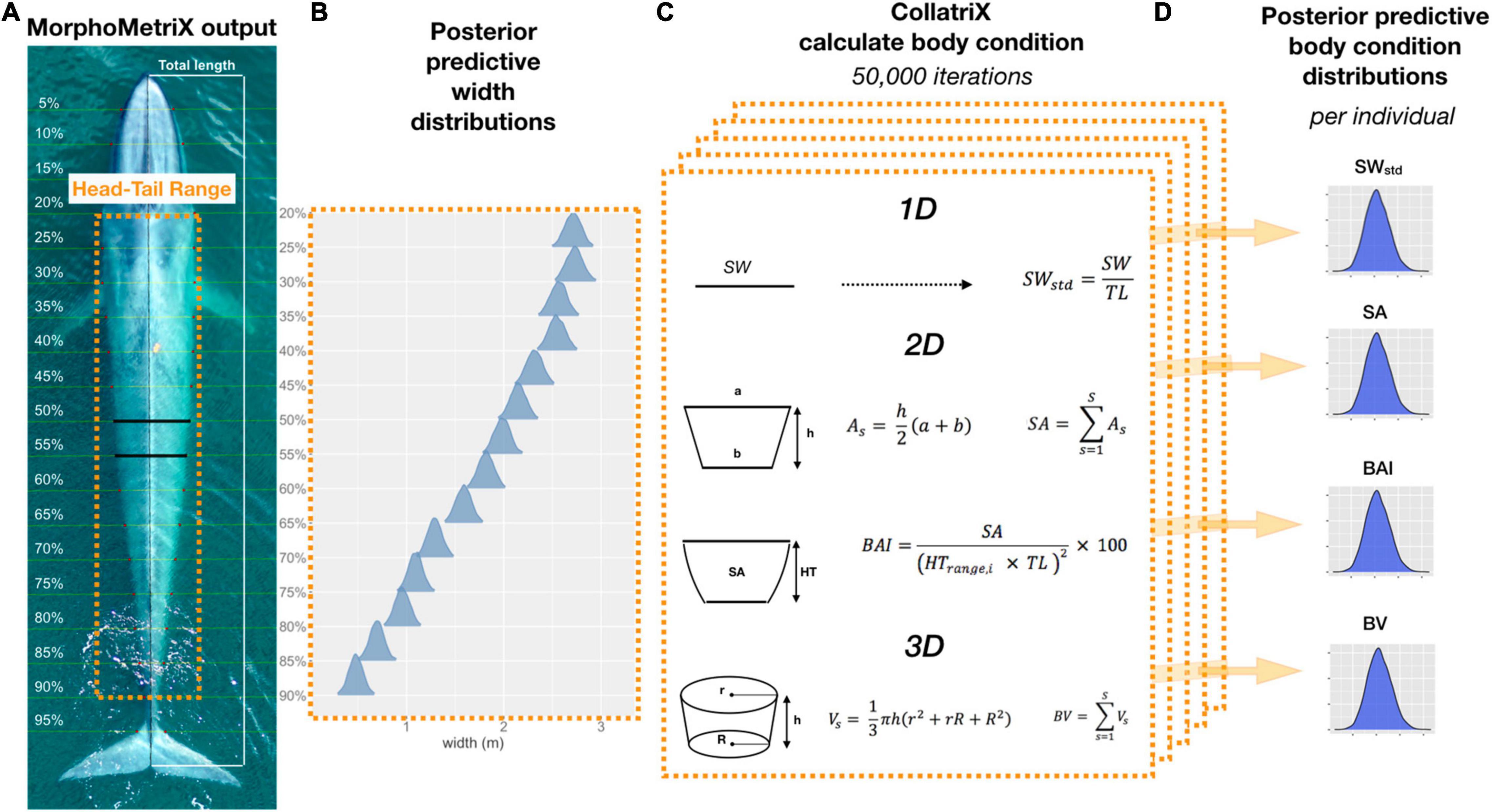
Figure 1. Overview of Bayesian framework for calculating the different body condition metrics in this study. (A) An example of a MorphoMetriX output (Torres and Bierlich, 2020) from a UAS image of a blue whale. Total length (TL) measured from rostrum to fluke notch with perpendicular widths segmented in 5% increments of TL. Head-Tail Range represents the region of the body that excludes the fins, head, and tail that will be used to calculate each body condition metric. (B) Posterior predictive distributions for each 5% width included in the Head-Tail Range (20–90%) that will be used to calculate each body condition metric. (C) One-dimensional (1D), 2D, and 3D body condition metrics are calculated using CollatriX (Bird and Bierlich, 2020) for each iteration in the MCMC output of the posterior predicted widths. (D) The posterior predictive distributions for each body condition metric calculated for a single individual. SW_std, standardized single width; SA, surface area; BAI, body area index; and BV, body volume.

One-dimensional estimates consist of a single body width measurement of an individual. One-dimensional approaches are simple, save analytical time, and can accurately reflect energy reserves (Miller et al., 2012; Fearnbach et al., 2018). For example, Miller et al. (2012) found that measurements of body widths were comparable to measurements of the girths of carcasses. Durban et al. (2016) demonstrated how a SW measure could distinguish between a “robust” and “lean” blue whale of similar length. Perryman and Lynn (2002) measured the maximum width of gray whales to show that individuals were thinner on their northbound migration to the feeding grounds than on their southbound migration to the breeding grounds. However, a 1D measurement requires knowledge of which width measurement best captures change along the body, which is something that may be more challenging for species with a data deficiency in morphometry (e.g., Hooker et al., 2019). One-dimensional approaches also risk missing subtle, but important, variation in energy reserves over the body (Lockyer, 1981; Miller et al., 2011, 2012; Christiansen et al., 2013, 2016).

In comparison, 2D and 3D estimates encompass variation along the body by measuring the total body length of the animal and then segmenting the animal into perpendicular and incremental width measurements, typically at increments of 5 or 10% of TL (Figure 1). Two-dimensional body condition measurements sum these width segments to calculate a projected dorsal SA (m²). This approach has been used to measure changes in body condition of humpback whales on the breeding and foraging grounds (Christiansen et al., 2016; Aoki et al., 2021). Cubbage and Calambokidis (1987) reported the first use of stereo-photogrammetry from airplanes to measure body length of bowhead whales in 3D images and demonstrated it had better precision than estimates from 2D images, though the authors noted the added complication of obtaining 3D measurements may not be worth the cost. Most UAS platforms are equipped with a single-camera and thus obtain 3D body condition estimates by measuring the width segments in the horizontal and vertical plane of the body to calculate total BV (m³) (Christiansen et al., 2018, 2020a,b, 2021). Volumetric models allow for estimation of body mass, which can then be used in energetic models to quantify energy storage in absolute standard units (Christiansen et al., 2019).

Both SA (2D) and BV (3D) are commonly used to calculate a body condition index (BCI), which represents the residuals from a linear regression between the 2D or 3D measurement and the TL of the animal. This approach has been used to compare relative body condition between different reproductive classes of humpback whales on the breeding grounds, as well as Southern and North Atlantic right whale populations (Christiansen et al., 2016, 2018, 2020a,b). Body area index (BAI) is a 2D standardized measurement of whale body condition developed based on the body mass index (BMI) that is commonly used for humans, where BMI = mass (kg)/height (m²) (Gallagher et al., 1996; Flegal et al., 2012). BAI uses SA as a surrogate for body mass and has been used to quantify variation in body condition in individual gray whales across multiple years (Burnett et al., 2018; Lemos et al., 2020). BAI is standardized by length and is thus unitless and scale invariant, facilitating comparisons of individuals and populations over time (Burnett et al., 2018).

Recently, Bierlich et al. (2021) developed a statistical model using training data of known-sized calibration objects to predict the length and associated uncertainty of unknown sized objects (e.g., whales). In the present study, we apply the model outputs from Bierlich et al. (2021) to aerial imagery collected via UAS to predict and compare uncertainty associated with 1D, 2D, and 3D photogrammetry-based body condition measurements in three baleen whale species of different sizes: blue, humpback, and Antarctic minke whales (AMWs; Balaenoptera bonaerensis).

The four objectives of the present study are to: (1) apply methods described in Bierlich et al. (2021) to incorporate uncertainty associated with multiple measurements of the same individual from image(s) to estimate the body condition of blue, humpback and minke whales; (2) compare how uncertainty scales across 1D, 2D, and 3D body condition measurements of these estimates; (3) compare precision in the posterior predictive distributions for each body condition estimate; and (4) compare how body condition indices are correlated for these species. The focus of our study is to shed light on how uncertainty scales across each body condition measurement to help guide other researchers to choose a method that best addresses their research objectives with the least uncertainty. Our study provides a framework for researchers to quantify and report measurement uncertainty associated with different body condition measurements and to facilitate collaboration and comparisons across studies.

Materials and Methods

Model Development and Overview

We followed the Bayesian statistical framework described in Bierlich et al. (2021) to incorporate TL and width measurements of each individual whale from single and multiple images. We used the freely available training data (Bierlich et al., 2020) used by Bierlich et al. (2021) for the UAS hexacopters FreeFly Alta 6 and LemHex-44 (see section “Error Estimation” for description of these UAS platforms) of known-sized floating calibration objects collected in Monterey, CA (length = 1.27 m), Beaufort, NC (length = 1.48 m), and along the Western Antarctic Peninsula (WAP; length = 1.33 or 1.40 m), for a total of 110 images. We first estimated the posterior probability distribution of photogrammetric error parameters (θ) for each UAS platform used in data collection using the calibration data of the known-sized objects (x) via

$f\left(\mathrm{\theta }|x\right)=\frac{f(x|\mathrm{\theta })f(\mathrm{\theta })}{f(x)},(1)$

where f(x|θ) is the likelihood function, f(θ) is the prior probability distribution that defines the potential range for θ, f(x) is the marginal distribution of the measurement data, and f(θ|x) is the posterior distribution that defines the likely range of θ given data x. We then used the posterior probability distribution for θ as prior information to form a posterior predictive distribution for TL and width measurements of the whale via

$f\left(x_{new}|x\right)=\int f(x_{new}|\mathrm{\theta })f(\mathrm{\theta }|x)d\mathrm{\theta },(2)$

where f(x_new|θ) is the likelihood function, and f(θ|x) is the posterior probability distribution estimated from the training data that is set as the new prior probability distribution. The posterior predictive distribution f(x_new|x) quantifies uncertainty for each measurement (TL and widths) of the whale, based on the measurement errors from the calibration data. The length and width posterior distributions are then used to calculate a posterior predictive distribution for each body condition metric for each individual.

Error Estimation

We designed the likelihood function based on the ground sampling distance (GSD) and length measurement in pixels (L_p) described in Bierlich et al. (2021), with the addition of including multiple measurements from single or multiple images to estimate body condition of individuals. We used the following photogrammetric equations,

$GS{D}_j=\frac{a_j}{f_c}\times \frac{S_w}{I_w},(3)$

$L_{p,k,i,j}=\frac{Lengt{h}_{k,i}}{GS{D}_j},(4)$

which relate the altitude a_j (the distance (m) from the camera to the object of interest in image j), to the focal length f_c of the camera (mm), the sensor width S_w of the camera (mm), the image width I_w in pixels, the exact pixel-length L_p,k,i,j of measurement k (i.e., total body length, 5% width, 10% width, etc.) of whale i in image j, and the exact, unknown Length_k,i in meters of measurement k for whale i. Errors related to the object positioning within the image frame and lens distortion for the cameras used in this study (see section “Error Estimation” for description of UAS cameras) were found to be negligible by Bierlich et al. (2021), and were thus not included in the model. The data x = ($a_{L,j}{}^{\prime }$, $a_{B,j}{}^{\prime }$, $L_{p,k,i,j}{}^{\prime }$) denotes the altitude as measured by a laser altimeter ($a_{L,j}{}^{\prime }$) and barometer ($a_{B,j}{}^{\prime }$), and the measured length in pixels ($L_{p,k,i,j}{}^{\prime }$), all measured values with some level of uncertainty from the exact values of a_j and L_p,k,i,j, respectively. We set a uniform prior distribution for a_j (min = 5 m and max = 130 m) to restrict the model to the altitude range of the UAS during image collection. We modeled the barometer and laser altimeter’s measurement error with a normal distribution around the true a_j,

$a_{L,j}{}^{\prime }\sim \text{N}(a_j,{\mathrm{\sigma }}_L^2),(5)$

$a_{B,j}{}^{\prime }\sim N(a_j,{\mathrm{\sigma }}_B^2),(6)$

with an inverse gamma prior distribution for the variance parameters ${\mathrm{\sigma }}_L^2$ and ${\mathrm{\sigma }}_B^2$ (shape = 2, rate = 1). Following Bierlich et al. (2021), we used the known length (L_co,i) of each calibration object i to calculate its true pixel length L_p,i,j by rearranging Eqs 3, 4:

$L_{p,i,j}=\frac{L_{co,i}\times f_c\times I_w}{a_j\times S_w}.(7)$

We model the measured pixel-length, $L_{p,i,j}{}^{\prime }$, for each calibration object i with a normal distribution

$L_{p,i,j}{}^{\prime }\sim \text{N}(L_{p,i,j},{\mathrm{\sigma }}_{Lp}^2),(8)$

with an inverse gamma prior distribution for ${\mathrm{\sigma }}_{Lp}^2$ (shape = 5, rate = 4). The relationship between L_p,I,j and a_j in Eq. 7 implies a joint distribution that is conditional on L_co,i and has the following structure

$f(a_{L,j}^{\prime },a_{B,j}^{\prime },L_{p,i,j}{}^{\prime }|\mathrm{\theta },L_{co,i})=\int f\left(a_j\right)f\left(a_{L,j}^{\prime }|a_j,\mathrm{\theta }\right)f(a_{B,j}^{\prime }|a_j,\mathrm{\theta })f(L_{p,i,j}{}^{\prime }|a_j,\mathrm{\theta },L_{co,i}\left)d\right(a_j),(9)$

where f(a_j) is the uniform prior for the true altitude, $f\left(a_{L,j}^{\prime }|a_j,\mathrm{\theta }\right)$ and $f\left(a_{B,j}^{\prime }|a_j,\mathrm{\theta }\right)$ are the densities for the measurement error distributions (Eqs 5, 6), respectively, and $f\left(L_{p,i,j}^{\prime }|a_j,\mathrm{\theta },L_{co,i}\right)$ is the measurement error distribution for the pixels (Eq. 8), in which the true altitude determines the true pixel measurement L_p,i,j via Eq. 7. Throughout, the parameter vector $\mathrm{\theta }=({\mathrm{\sigma }}_L^2,{\mathrm{\sigma }}_B^2,{\mathrm{\sigma }}_{Lp}^2)$ contains the measurement error parameters. We then use measurements of L_co,i as training data to estimate the error parameters.

Measurement Predictions

We can now make inferences about multiple measurements of an unknown sized object (L_new), i.e., a whale, which are conditional on a new set of measurements ($a_{new}^{\prime }$ and $L_{p,new}^{\prime }$) and the error parameter estimates (θ). We assume L_new is independent from the training data and thus has the following conditional structure

$f\left(L_{new,k,i,j}|a_{B,new,j}^{\prime },a_{L,new,j}^{\prime },L_{p,new,k,i,j}^{\prime },\mathrm{\theta }\right)\propto f(a_{B,new,j}^{\prime },a_{L,new,j}^{\prime },L_{p,new,k,i,j}^{\prime }|L_{new,k,i,j},\mathrm{\theta })f(L_{new,k,i,j}),(10)$

where each L_new of measurement k for individual i in image j is calculated using Eqs 3, 4 with an assumed gamma prior distribution for the unobserved, true L_new (shape = 4.0, rate = 0.0013) (Bierlich et al., 2021). This model structure allows for multiple measurements (i.e., TL and widths) to be estimated from a single image, as well as repeated measurements across multiple images, of the same whale. The final model output produces a single posterior predictive distribution of each measurement for each individual. We then use the posterior predictive TL and width distributions to calculate body condition metrics described in section “Body Condition Metrics.”

Model development and analyses were conducted in R (Version 4.0.2, R Core Team, 2020) using the drake package (Landau, 2018). Estimation and prediction were performed using Markov Chain Monte Carlo (MCMC) sampling in NIMBLE (de Valpine et al., 2017) with 1,000 burn-in followed by 1,000,000 iterations with a thinning rate of every 10th sample. Three independent chains were run to confirm consistency between runs and inspected visually for convergence. The model was validated by randomly sampling half of the training data (x) and then using the error parameters to predict the length measurement for the remaining half to compare with the known length of the calibration object (Bierlich et al., 2021).

Testing Data

Unoccupied Aircraft Systems Data Collection

We used the model to predict TL and width measurements of blue, humpback, and AMWs from high resolution images collected using two hexacopters: a Mikrokopter LemHex-44 and FreeFly Alta 6. Both UAS platforms contained an onboard barometer and were fitted with a LightWare SF11/C laser altimeter, as well as a Sony Alpha a5100 camera with an APS-C (23.5 × 15.6 mm) sensor, 6,000 × 4,000 pixel resolution, and either a 35 or 50 mm Sony SEL f_c. Images were collected between 2017 and 2019 along the coast of Monterey, CA (blue whales) or the WAP (humpbacks and AMWs).

Data Filtering

The best images were selected for each individual and ranked for quality in measurability following Christiansen et al. (2018), where a score of 1 (good quality), 2 (medium quality), or 3 (poor quality) was applied to seven attributes: camera focus, straightness of body, body roll, body arch, body pitch, TL measurability and body width measurability. Images with a score of 3 in any attribute were removed from analysis, as well as any images that received a score of 2 in both roll and arch, roll and pitch, or arch and pitch (Christiansen et al., 2018). Measurements from up to five images collected during the same flight were used per individual.

As in Bierlich et al. (2021), the model was designed to accommodate images with altitude readings from both the barometer and laser simultaneously, or from either in isolation [e.g., caused by a missing (NA) altitude value for the laser or barometer]. For images with an altitude difference >10% between the barometer and laser altimeter, barometer values were changed to NA, as results from Bierlich et al. (2021) showed that measurements with NA barometer values yielded similar results to those when both laser and barometer were included.

Photogrammetry

We used MorphoMetriX (v1.0.2) open-source photogrammetry software (Torres and Bierlich, 2020) to measure (in pixels) the TL (tip of rostrum to fluke notch) and perpendicular widths in 5% increments of the TL measurement (Figure 1). MorphoMetriX outputs were collated using CollatriX (v1.0.7) (Bird and Bierlich, 2020), and then input into the uncertainty model. As demonstrated by Christiansen et al. (2018), initial analysis of individuals with measurements from multiple images (see section “Data Filtering”) confirmed that filtering for images with quality scores of 1 or 2 was robust to potential biases of width measurements related to variation in TL measurements, such as from any slight bending or arching of the individual (Supplementary Figure 1).

Body Condition Metrics

Selecting Head-Tail Range

We define body condition as a morphological measure of an individual’s relative energy reserves compared to its structural size (Peig and Green, 2009). Green (2001) noted that it is imperative to separate effects of structural size of the body from the size of the energy capital, as both aspects can have major consequences for fitness, survival rates, and habitat use. Therefore, an initial goal of any study of body condition should be to identify the body components that best reflect variation in energy reserves. Intra-seasonal changes in energy storage are not exhibited homogenously over the body of baleen whales, and are species specific (Lockyer, 1981; Miller et al., 2012; Christiansen et al., 2013). Cetaceans do not store energy reserves in their pectoral fins, head, or tail flukes (Brodie, 1975; Lockyer, 1981; Koopman et al., 2002). This pattern was also confirmed photogrammetrically by Christiansen et al. (2016), who found no intra-seasonal variation in the width of the head or the lower section of the peduncle across all reproductive classes of humpback whales. Thus, we used the width range along the body between the head and tail of each individual, which we refer to as the “Head-Tail Range,” to encompass changes in energy storage (Figure 1). To account for potential individual variation across and within species, we assigned a Head-Tail Range specific to each individual to ensure that the range used to calculate each body condition metric captured the relative energy stores for that individual. The boundary of the head was based on the location of the eyes to the nearest perpendicular width, and the boundary for the tail was determined as the nearest perpendicular width to the start of the peduncle (Figure 1). The Head-Tail Range was 20–90% for blue whales, 20–85% for AMWs, 25–85% for juvenile and mature humpback whales, and 20–85% for humpback whale calves (Table 1).

TABLE 1

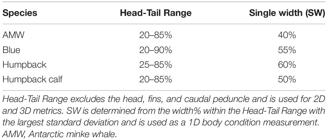
Table 1. The Head-Tail Range and single width (SW) measurement for each species used for measuring body condition.

One-Dimensional: Single-Width (SW_std)

The SW measurement, assessed as the 1D body condition estimate, was defined as the perpendicular width measurement within the Head-Tail Range that had the largest standard deviation across individuals in each species. Thus, the SW measurement is species-specific and should capture the greatest variation in width amongst individuals within that species (Miller et al., 2012; Durban et al., 2016; Figure 1). The SW measurement was 40% for AMWs, 55% for blue whales, 60% for humpback whales, and 50% for humpback whale calves. We then standardized each SW measure, SW_std, by the TL of the individual (Miller et al., 2012; Fearnbach et al., 2018),

$S{W}_{std}=\frac{SW}{TL}.(11)$

Two-Dimensional: Projected Dorsal Surface Area

The Head-Tail Range for each individual was used to calculate the projected dorsal SA following Christiansen et al. (2016). SA was modeled as a series of trapezoids connected at each width measurement site (Figure 1), where the SA (m²) of each trapezoid segment, A_s, was calculated using

$A_s=\frac{h}{2}\left(a+b\right),(12)$

where a is the anterior base (width) of a trapezoid segment, b is the posterior base (width) of a trapezoid segment and h is the distance between both width measurement sites (h = 0.05 × TL) (Figure 1). The total SA (m²) for each individual was calculated by summing the area of each trapezoid segment, A_s, within the Head-Tail Range,

$SA=\sum _{s=1}^S{A}_s,(13)$

where S is the total number of trapezoid segments within the Head-Tail Range.

Two-Dimensional: Body Area Index

Surface area was also used to calculate BAI, but instead of modeling each perpendicular width segment as a series of trapezoids (as in Eqs 12, 13), a parabola was fit through each perpendicular width point within the Head-Tail Range on each side of the whale (see Burnett et al., 2018). The SA was then calculated as the area under each parabola and used to calculate BAI by

$BAI=\frac{SA}{{\left(HT\times TL\right)}^2}\times \mathrm{\hspace{0.33em}100},(14)$

where HT is the Head-Tail Range of the individual (i.e., 0.70 for a Head-Tail Range between 20 and 90% as in Figure 1) and the multiplication by 100 allowed for a more intuitive value (>1.0). A linear regression between the trapezoidal SA calculated in Eq. 13 and the parabolic SA calculated in Eq. 14 yielded an r² = 0.99, suggesting that these two methods for calculating SA are virtually identical.

Three-Dimensional: Body Volume

Body volume was modeled as a series of frustums (truncated cones) connected at each perpendicular width measurement site following Christiansen et al. (2018; Figure 1). The cross-section of each frustum was assumed to be circular and the volume of each frustum segment, V_s, was calculated by

$V_{s,i,k}=\frac{1}{3}\mathrm{\pi }h\left(r_{i,k}{}^2+r_{i,k}{R}_{i,k}+R_{i,k}{}^2\right),(15)$

where h is the distance between both body width measurement sites (h = 0.05 × TL), r is the radius of the anterior girth measurement of the frustum (i.e., half the anterior width measurement), and R is the radius of the posterior girth measurement of the frustum (i.e., half the posterior width measurement). The total body volume, BV (m³), was then calculated from the summation of all the frustum segments within the Head-Tail Range

$B{V}_i=\sum _{s=1}^S{V}_s(16)$

where S is the total number of frustum segments within the Head-Tail Range.

Predicted Body Condition Posterior Distributions

Each of these body condition measurements were calculated in each MCMC iteration for each whale (n_iterations = 50,000, after excluding first half as burn-in). This yields the posterior predictive distribution of SW, SW_std, SA, BAI, and BV for each individual (Figure 1). We then calculated the mean and 95% highest posterior density (HPD) interval for each posterior distribution (Figure 1). The 95% HPD interval represents the shortest interval containing 95% of the posterior distribution’s mass, and ultimately serves as the measure of uncertainty around each measurement prediction (Bierlich et al., 2021).

Body Condition Index

The mean of the predictive posterior distributions for SA and BV were then used to calculate the BCI following methods from Christiansen et al. (2018). BCI_SA was calculated as

$BC{I}_{SA,i}=\frac{S{A}_{obs,i}-S{A}_{exp,i}}{S{A}_{exp,i}}(17)$

where SA_{obs,  i} is the observed mean of the posterior predictive distribution of SA for whale i, and SA_{exp,  i} is the expected SA for whale i from a linear relationship between SA_{obs,  i} and the observed mean of the posterior predictive distribution of TL for whale i, on a log-log scale.

Likewise, BCI_BV was calculated using

$BC{I}_{BV,i}=\frac{B{V}_{obs,i}-B{V}_{exp,i}}{B{V}_{exp,i}}(18)$

where BV_{obs,  i} is the observed mean of the posterior predictive distribution of BV for whale i, and BV_{exp,  i} is the expected BV for whale i from the linear relationship between BV_{obs,  i} and observed mean of the posterior predictive distribution of TL for whale i, on the log-log scale. It has been assumed that a positive BCI value reflects an animal in “good” condition, while a negative value indicates an animal in “poor” condition for that population (Christiansen et al., 2018, 2020a).

Statistical Analysis

For the purposes of this study, we intentionally ignored considerations of when each whale was sampled (e.g., day within season, year), as our focus was on comparing the different methods for measuring body condition rather than understanding the ecological context of these measurements.

Scaling

To analyze how uncertainty scaled across 1D, 2D, and 3D measurements, we analyzed the linear relationship between the standard deviation of the posterior predictive distribution for each unstandardized body condition measurement (SW, SA, and BV) of each individual on a log-log scale.

Precision

We also compared the precision of the posterior predictive distributions for each body condition measurement (SW, SW_std, SA, BAI, and BV). The National Institute of Standards and Technology (NIST) defines precision as the closeness of agreement between independent measurements of a quantity under the same condition (Taylor and Kuyatt, 1994). Precision is a measure of how well a measurement can be made without reference to a true value, while uncertainty incorporates the range of values in the distribution that is expected to contain the true value. The true body condition of each individual in this study is not known, but precision can help identify a metric’s ability to detect small changes in body condition amongst individuals. As each metric varies in measured units, i.e., unitless, m, m², and m³, we analyzed the precision of each metric by calculating the coefficient of variation (CV%) as

$C{V\%}_{i,m}=\left(\frac{{\mathrm{\sigma }}_{i,m}}{{\mathrm{\mu }}_{i,m}}\right)\times 100(19)$

where σ is the standard deviation and μ is the mean of the posterior predictive distribution for each body condition metric m of individual i.

Correlation

We used a correlation matrix and linear regression with Pearson’s correlation coefficient r to analyze the relationship between each standardized BCI (SW_std, BAI, BCI_SA, and BCI_BV). All analyses were conducted in R (Version 4.0.2, R Core Team, 2020).

Results

After filtering for image quality, we used photogrammetric measurements of 127 whales for the analysis: 32 blue whales, 40 AMWs, and 55 humpback whales (including 15 calves). The absolute and relative (standardized) perpendicular widths of each species varied, illustrating differences in body shapes (Figure 2).

FIGURE 2

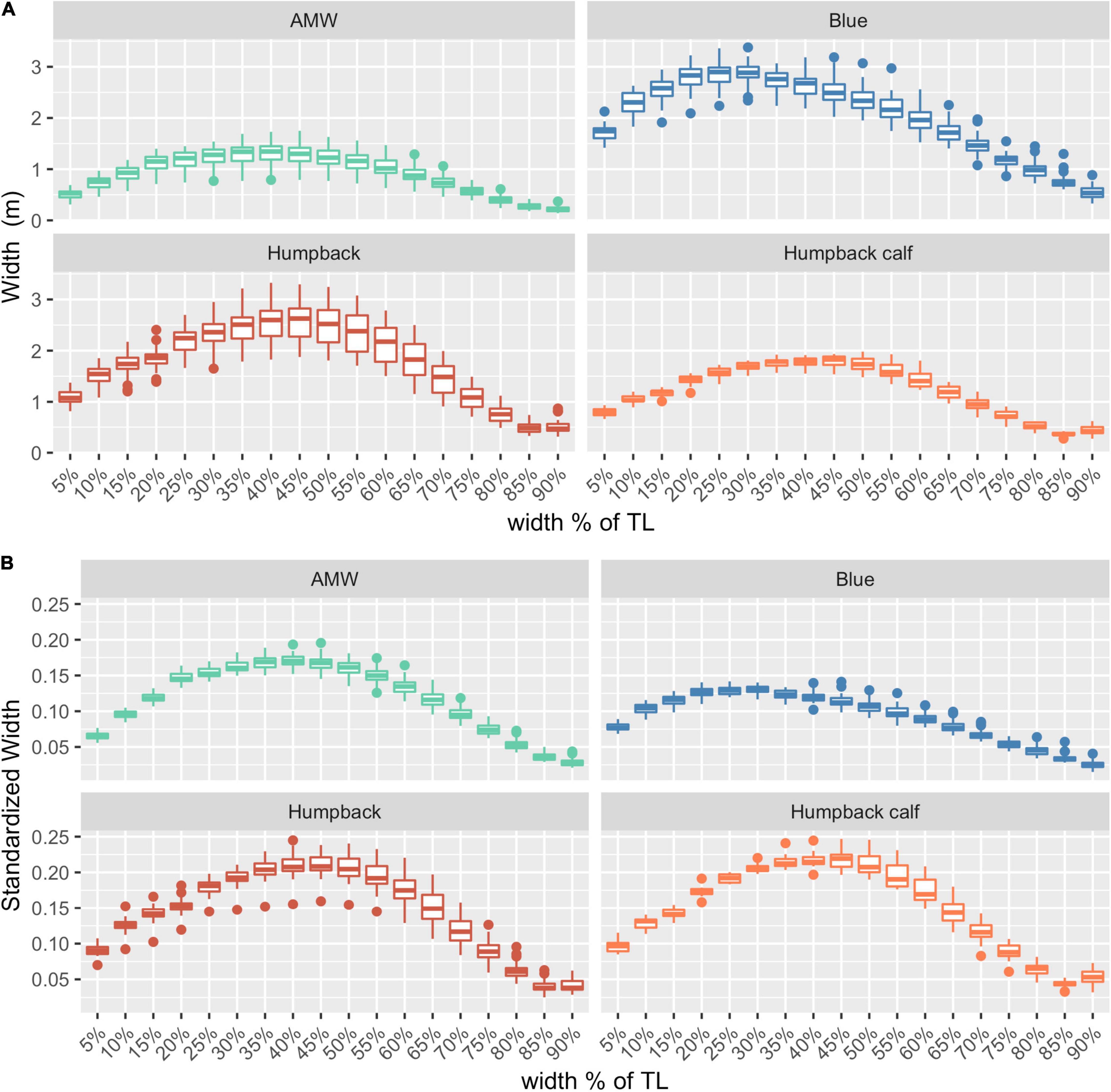
Figure 2. Body shapes for each species. (A) Absolute widths (m), (B) relative widths, standardized by dividing each width by the total length of the individual. AMW, Antarctic minke whale (n = 40), blue whales (n = 32), humpback (n = 40), and humpback calves (n = 15). The middle line in each box represents the median, or second quartile (50th percentile), the lower and upper hinge of the box represent the first and third quartile (the 25th and 75th percentile), respectively, and the lower and upper whisker represents the smallest and largest value that extend at most 1.5 × IQR, where IQR is the interquartile range. Any data beyond these whiskers are considered outlying points and plotted individually.

Body Condition Measurements

The posterior predictive distribution of TL and each body condition measurement were calculated for each individual whale (Figure 3 provides an example output for an individual blue whale). Both the Head-Tail Range and SW captured variability in body condition amongst individuals in each species, as well as across species (Table 2 and Figure 4). As expected, SW, SA, and BV increased as the TL increased for each species, while SW_std and BAI did not because they are standardized by TL (Figure 4). Despite being almost 10 m shorter than blue whales, humpback whales displayed similar and greater SW measurements (absolute width) (Figures 2, 4). Overall, blue whales had smaller SW_std (relative width) and a lower BAI range compared to humpback and minke whales (Figure 4), reflecting differences in their body shapes (Figure 2). Each species clearly displayed its own unique range of BAI values, with little overlap amongst species, suggesting that this measurement of body condition is species-specific (Figure 4 and Table 2). There was more overlap in SW_std values between AMW and humpback whales, especially with humpback whale calves (Figure 4 and Table 2).

FIGURE 3

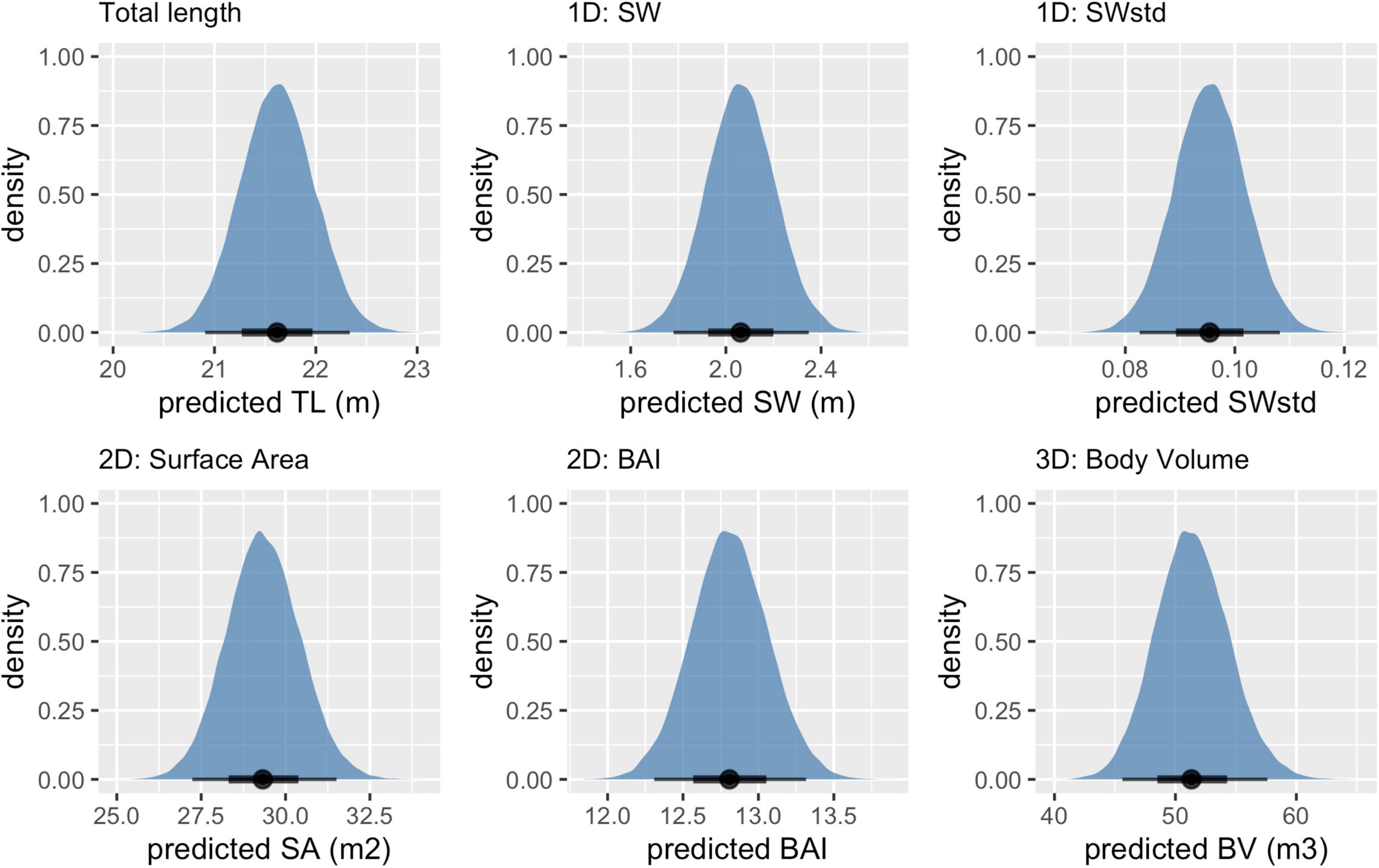
Figure 3. Example of posterior predictive distributions of measurements and associated uncertainty from UAS images of an individual blue whale. Measurements include total length (TL), single-width (SW), single-width standardized (SW_std), surface area (SA), body area index (BAI), and body volume (BV). The longer thin black bars represent the 95% HPD interval, the thicker shorter black bars represent the 65% HPD interval, and the black dot represents the mean value. Note that each x-axis is on a different scale.

TABLE 2

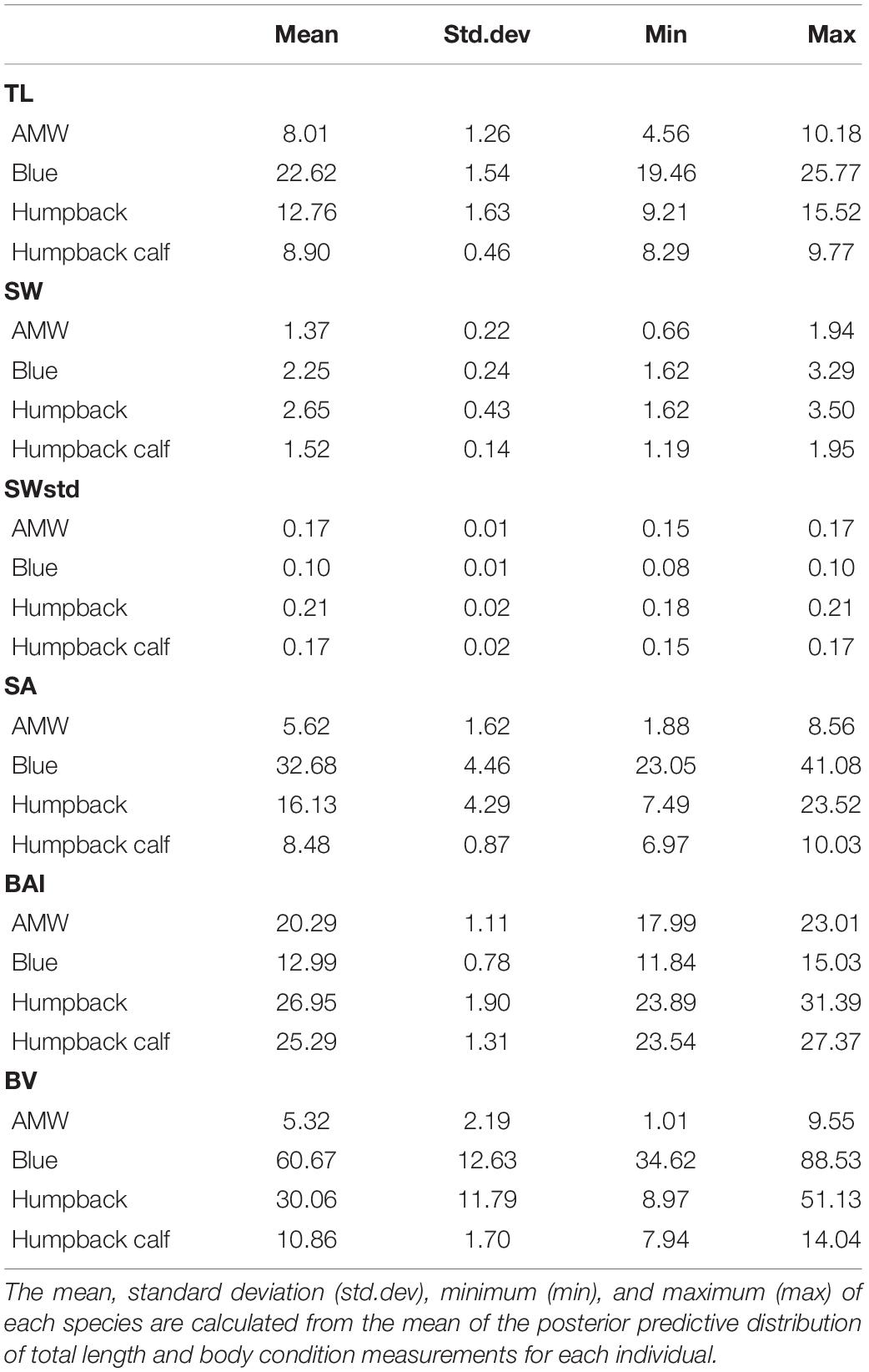
Table 2. Summary of each body condition measurement for each species.

FIGURE 4

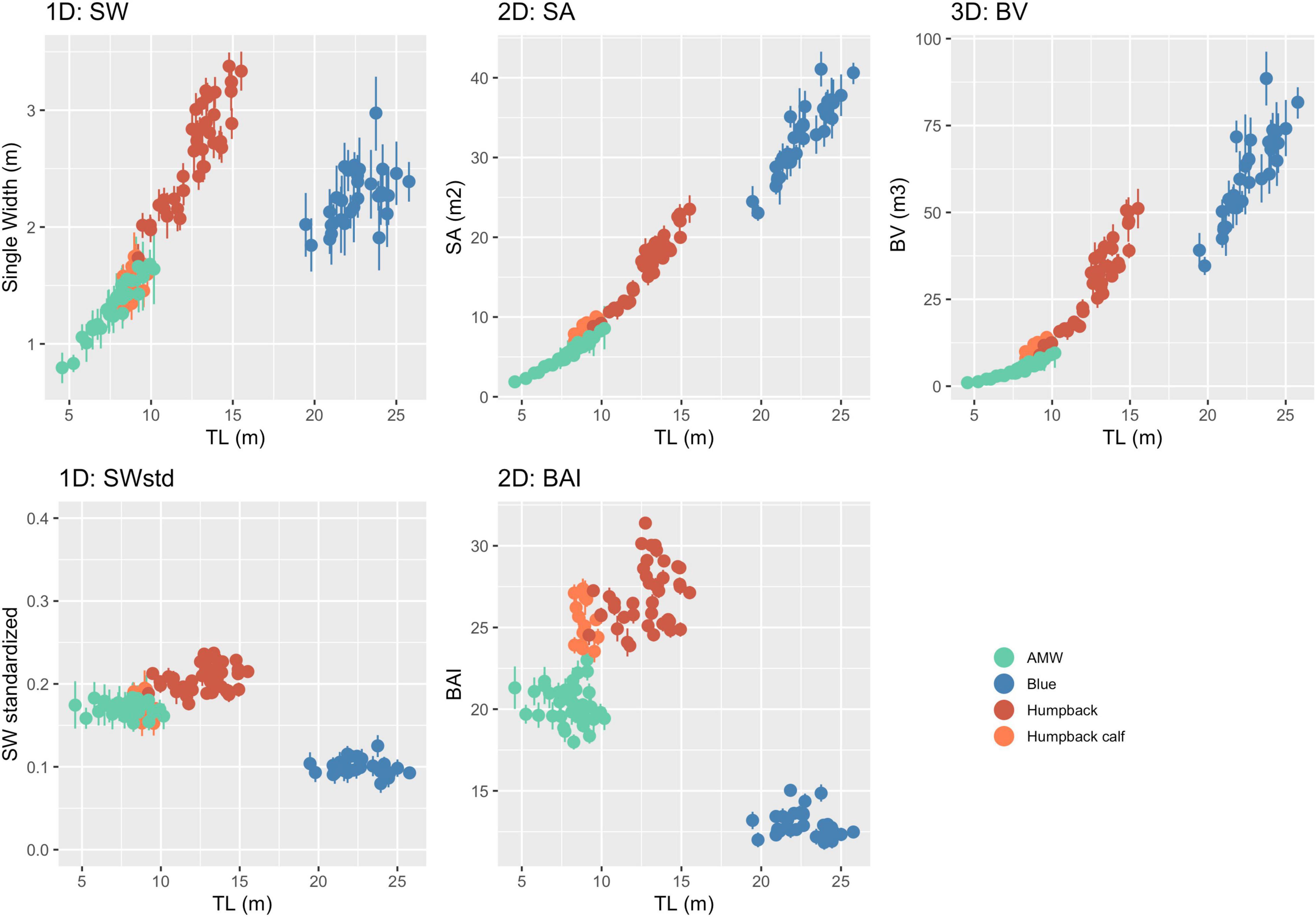
Figure 4. One-dimensional (1D), 2D, and 3D body condition measurements with uncertainty. Each point represents the mean of the posterior predictive distribution of that body condition measurement with the bars representing the lower and upper bounds of the 95% HPD interval for that specific individual whale (represented in Figure 3). Unstandardized measurements are in the top three panels, while the bottom two panels are standardized versions of 1D and 2D measurements.

Scaling of Uncertainty

Overall, uncertainty associated with 2D and 3D body condition measurements increased at a greater proportion than uncertainty associated with 1D measurements (Figure 5). For every unit of increase in 1D uncertainty, 2D uncertainty increased by 1.45 (CI: 1.20, 1.69) and 3D uncertainty increased by 1.76 (CI: 1.39, 2.13) (Figure 5).

FIGURE 5

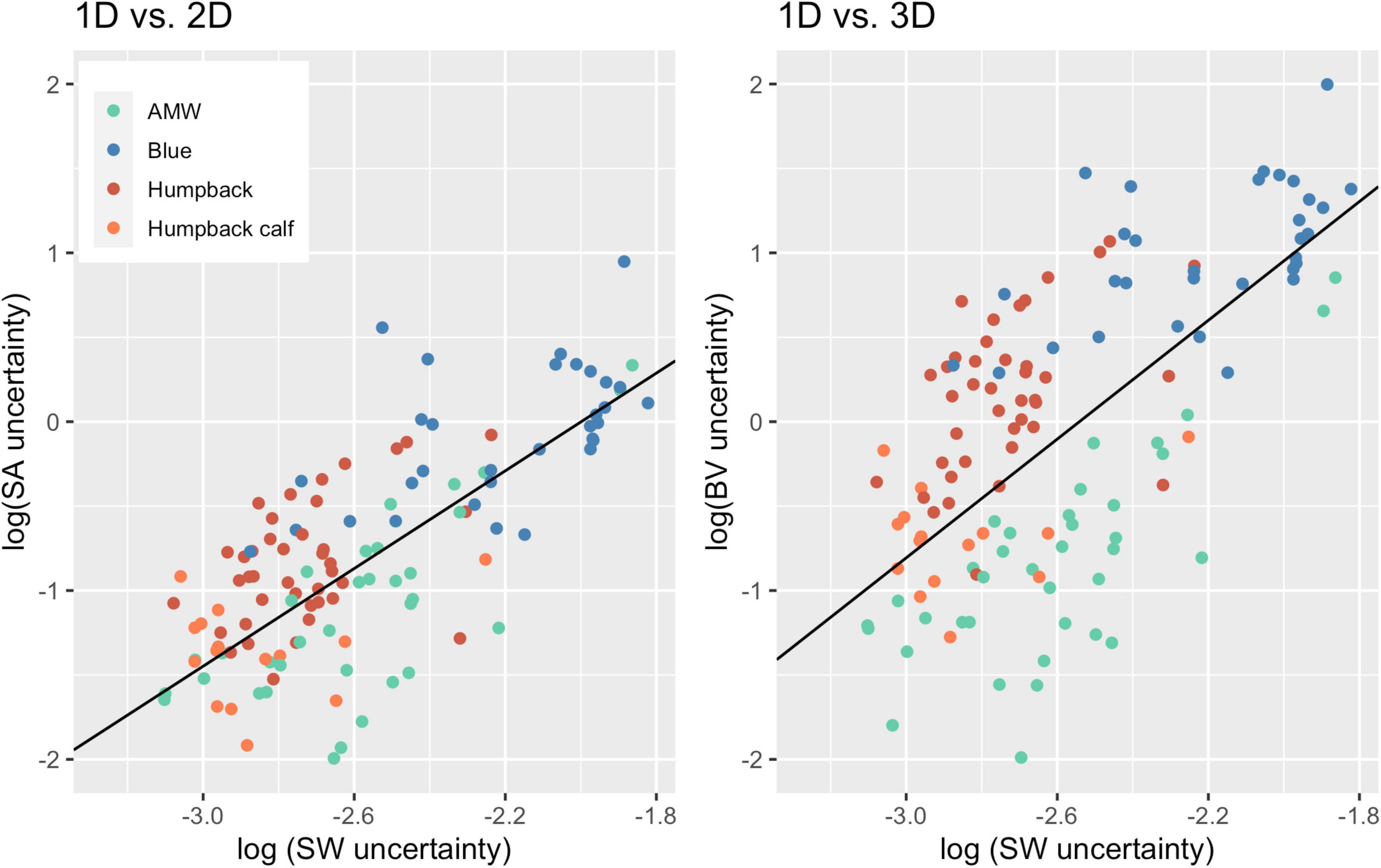
Figure 5. Scaling of 2D and 3D uncertainty with 1D uncertainty. Each point represents an individual whale and the uncertainty (defined here as the SD of the posterior predictive distribution for each metric), associated with 1D, 2D, and 3D body condition metrics. The black lines represent the linear regression for uncertainty between 1D and 2D (slope = 1.45; CI: 1.20, 1.69; intercept = 2.89) and 1D and 3D (slope = 1.76; CI: 1.39, 2.13, intercept = 4.47). Data from 40 Antarctic minke whales (AMW), 32 blue whales, 40 humpback whales, and 15 humpback whale calves.

Precision

The precision of each body condition measurement was calculated as the CV% (Eq. 19) to analyze the closeness in agreement of the posterior predictive distribution for each individual. In other words, CV% compares the relative width of the predictive posterior distributions of each body condition measurement for each individual (i.e., the distributions illustrated in Figure 3). BAI was the most precise measure with the smallest CV% (CV%: mean = 1.31%, SD = 0.53%) (Table 3 and Figure 6). Thus, in theory, BAI should be able to detect smaller changes in body condition than the other measurements. SW_std was the second most precise measurement (CV%: mean = 3.73%, SD = 1.65%), followed by SA (CV%: mean = 4.01%, SD = 2.82%), SW (CV%: mean = 4.29%, SD = 1.83%), and finally BV (CV%: mean = 6.2%, SD = 4.21%) (Table 3 and Figure 6).

TABLE 3

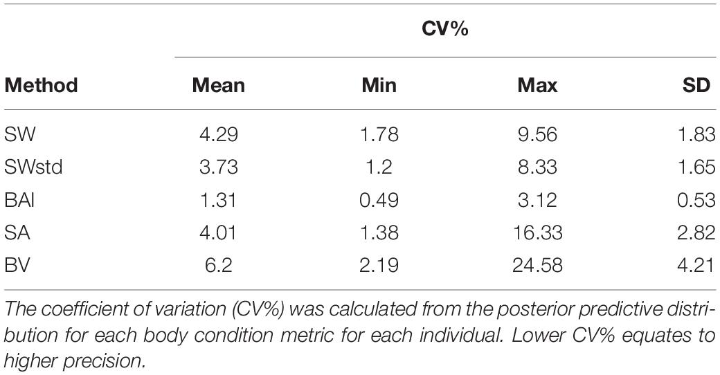
Table 3. Comparison of metric precision.

FIGURE 6

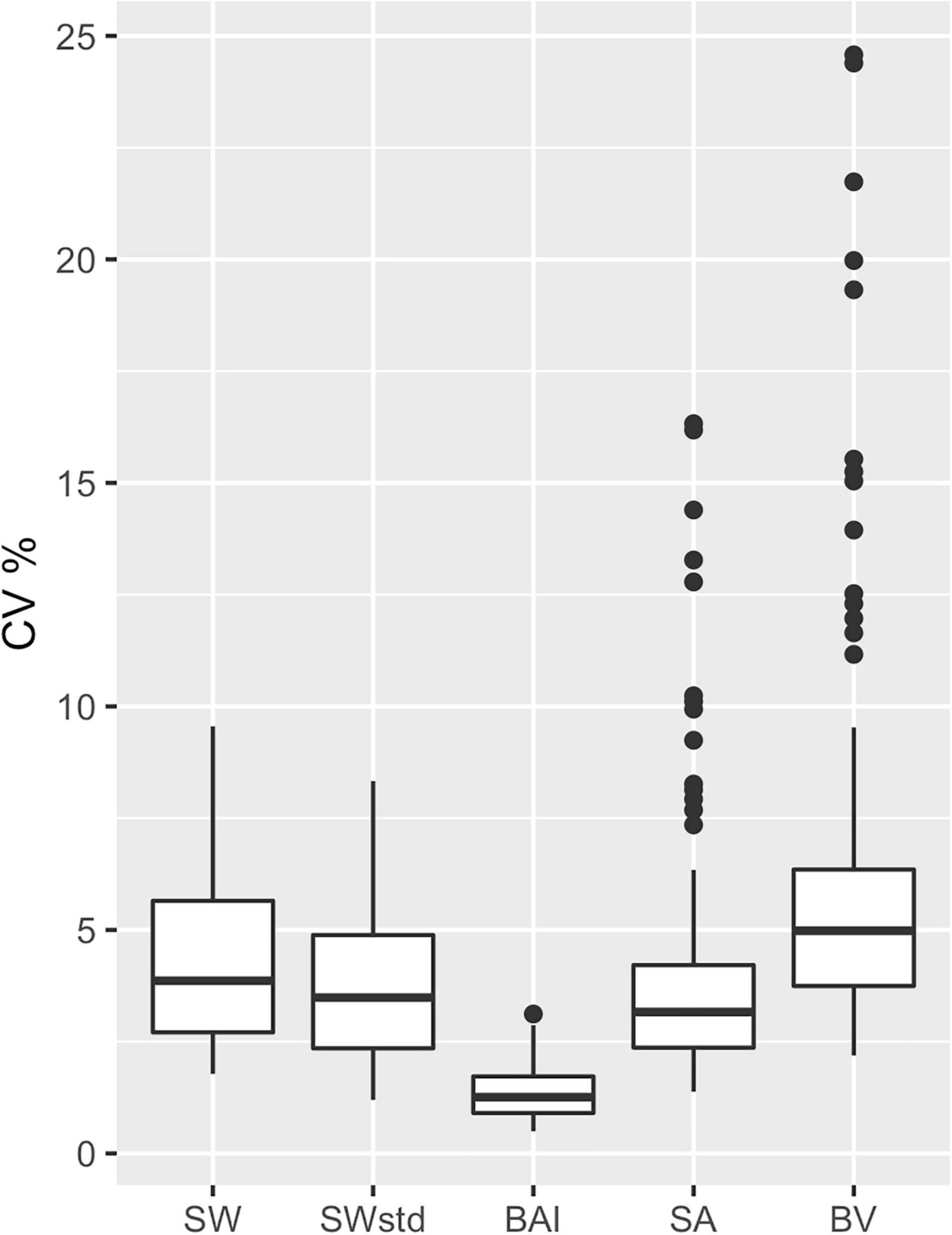
Figure 6. Comparison of metric precision. The coefficient of variation (CV%) was calculated from the posterior predictive distribution for each body condition metric for each individual. SW, single width (1D); SW_std, standardized single width (Eq. 11) (1D); BAI, body area index (2D) (Eq. 14); SA, surface area (2D) (Eq. 13); and BV, body volume (Eq. 16). The middle line in each box represents the median, or second quartile (50th percentile), the lower and upper hinge of the box represent the first and third quartile (the 25th and 75th percentile), respectively, and the lower and upper whisker represents the smallest and largest value that at extend at most 1.5 × IQR, where IQR is the interquartile range. Any data beyond these whiskers are considered outlying points and plotted individually.

Correlation

Each standardized body condition measurement (SW_std, BAI, BCI_SA, and BCI_BV) was highly correlated across species (Figure 7), demonstrating that each of these standardized body condition measurements provides similar information. AMWs had the strongest relationship between each metric (all r > 0.93), followed by adult humpback whales (all r > 0.92), humpback calves (r > 0.88), and blue whales (r > 0.87) (Figure 7). Both BCI_SA and BCI_BV were consistently the most correlated across each species (all r > 0.99) (Figure 7). BAI showed slightly higher correlation with each metric for each species (all r > 0.88) compared to SW_std, BCI_SA, and BCI_BV (all r > 0.87) (Figure 7).

FIGURE 7

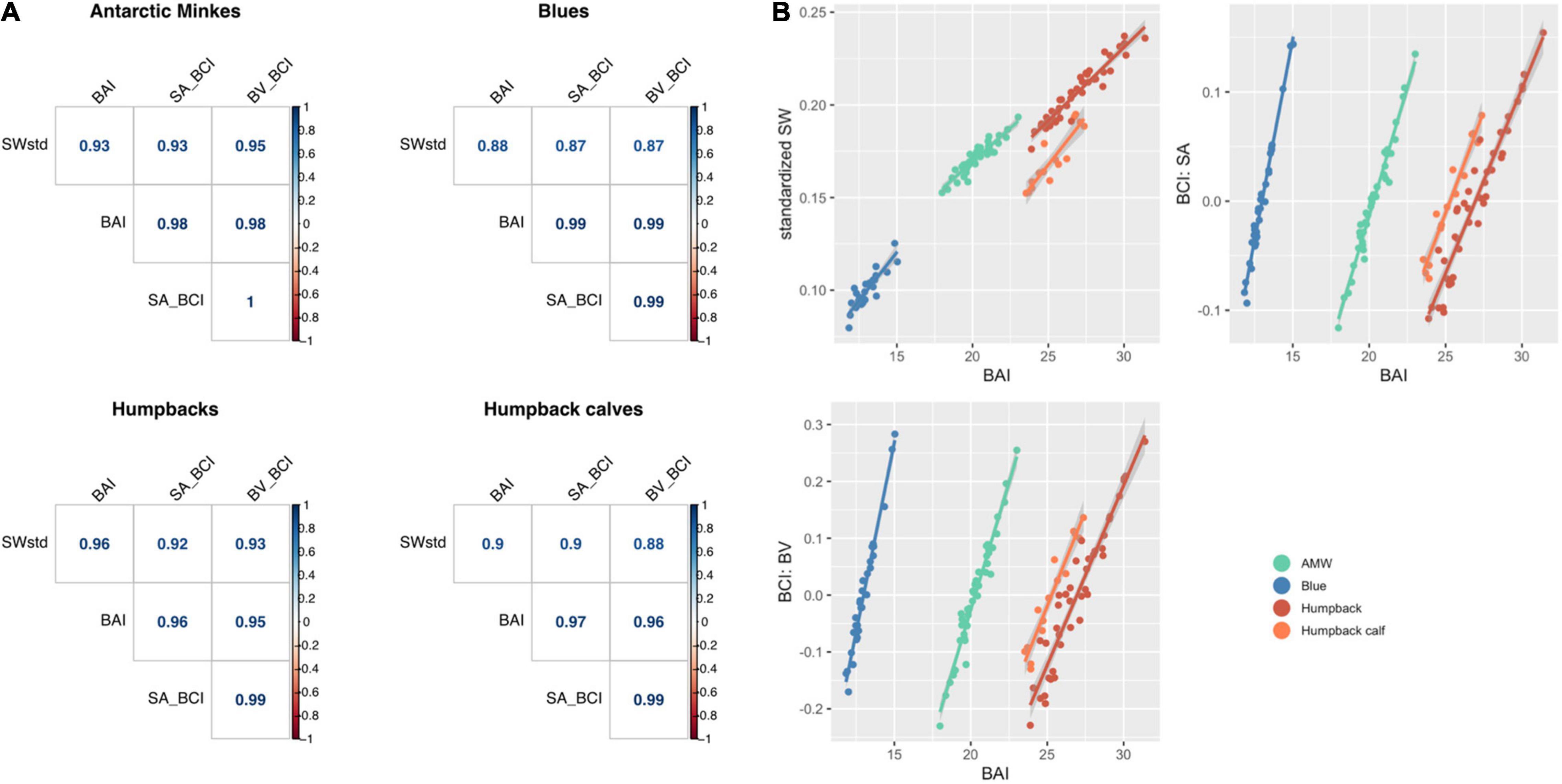
Figure 7. (A) Correlogram (graph of correlation matrix) comparing each standardized metric for each species. SW_std, standardized single width (Eq. 11); SA_BCI, BCI_SA (Eq. 17); BV_BCI, BCI_BV (Eq.18); BAI, body area index (Eq. 14). (B) Regression between BAI and each standardized metric. BAI is highly correlated with each standardized metric, with Pearson’s correlation coefficient r > 0.88 for each comparison.

Discussion

Here we present the first comparison of 1D, 2D, and 3D photogrammetry-based body condition estimates of baleen whales, while incorporating the uncertainty associated with each estimate. This study builds on the Bayesian statistical framework described in Bierlich et al. (2021); this framework allows us to incorporate multiple measurements (i.e., body length and width) of the same individual whale from a single image, as well as across multiple images, in order to creat posterior predictive distributions for body condition. Our study serves as a guide to help researchers select the most appropriate body condition measurement for their study and incorporate photogrammetric uncertainty associated with these measurements to yield robust scientific conclusions and facilitate collaboration and comparisons across studies. Data and model code are available at https://github.com/KCBierlich/Body_Condition_Analysis.

Scaling of Uncertainty

Uncertainty does not scale linearly across 1D, 2D, and 3D body condition metrics. Just as scaling relationships between multi-dimensional shapes do not change in the same ratio as their linear dimensions (Schmidt-Nielsen, 1984), uncertainty associated with 2D and 3D measurements of these three whale species increases by a factor of 1.45 and 1.76 compared to 1D measurements, respectively (Figure 5). This is an important finding, as utilizing a multi-dimensional body condition measurement may incur a higher cost of increased uncertainty. Thus, studies should consider the potential added cost of uncertainty when choosing a body condition measurement. For example, if a project is primarily aimed at measuring relative body condition change for a given baleen whale species, it may be best to use a 1D or 2D measurement to yield results with less uncertainty. However, calculating BV is often a preferred metric if the project goal necessitates approximation of whale body mass (Schmidt-Nielsen, 1984), which can be applied to quantify the maternal cost of reproduction (Christiansen et al., 2018) and estimate body mass (Southern right whales; Christiansen et al., 2019). BV has also been useful for studies comparing locomotion and hydrodynamic performance across baleen whale species (Woodward et al., 2006). In this paper we compared ways to calculate BV from 2D measurements but did not have actual 3D measurements which could have potentially improved the calculation of BV. However, as demonstrated in Cubbage and Calambokidis (1987), the complication and cost of obtaining actual 3D measurements may not be cost-effective. Bierlich et al. (2021) found that measurement error varies depending on the camera, focal length lens, altimeter, and altitude, so studies calculating BV can help mitigate relatively higher rates of associated uncertainty by selecting a UAS platform with sensors that yield low uncertainty and implementing strict field protocols to further minimizes errors.

The goal of our study was to describe broad trends in how uncertainty scales across different body condition measurements rather than a detailed comparison between species, but it is interesting to note that uncertainty appears to scale differently for each species, which likely contributed to the wide confidence intervals observed (Figure 5). For instance, adult humpback whales had greater uncertainty in SA and BV measurements compared to the other species (Figure 5). This variation is likely due to differences in body shape (Figure 2). For example, humpback whales have larger absolute and relative widths compared to blue whales along the mid-line of the body, despite being almost 10 m shorter (Table 2 and Figures 2, 5). Humpback whales also displayed the largest variation in body widths compared to AMWs and blue whales (Table 2 and Figure 2). Overall, each species followed the broader trend of increasing uncertainty with a similar positive slope, and these slight variations in scaling can be further studied using interaction effects.

Comparing Body Condition Change

In measuring relative body condition change, BAI was the most precise measurement, followed by standardized single-width (SW_std) (Table 3 and Figure 6). SW_std provides a time saving advantage, as it only requires a single measurement, reducing the time spent performing and processing measurements. Hence, SW_std may be useful for pilot or exploratory studies of body condition. However, a SW measure may miss other widths that may contribute to the body condition of an individual. For example, while SW uses the perpendicular width with the largest standard deviation for each species, neighboring widths also display high variation and may collectively better contribute to the quantification of an individual’s condition (Figure 2). This is likely the reason why AMW and humpback whale calves had more overlap in their range of SW_std measurements than in BAI (Figure 4 and Table 2). Thus, a 2D standardized metric, such as BAI, which captures this potential variation along the body, may be a preferred metric. Studies interested in a standardized volumetric approach, especially as imagery is collected on the lateral height of the animal, could incorporate a body volume index (BVI), where BV is divided by the cube of the Head-Tail Range multiplied by the TL.

In comparing BCI_SA and BCI_BV with the mean posterior predictive distributions for SW_std and BAI, each of these standardized metrics are highly correlated with one another (Figures 4, 7). This correlation is an important finding, as it suggests that 1D, 2D, or 3D standardized metrics will draw similar relative predictions for body condition of individuals. In other words, researchers can be confident that similar conclusions will be drawn pertaining to the relative body condition of individuals in a study, regardless of which standardized metric they use. However, researchers should still expect differences in the uncertainty associated with these different measurements and employ the approach best suited to their research question and study species.

Advantages of Body Area Index for Detecting Body Condition Change

All standardized measurements were highly correlated with one another, but there were several clear advantages for using BAI in studies of variation in body condition. BAI incorporates multiple perpendicular widths to capture potential variation along the body and was the most precise measure across species, with a CV% range between 0.40 and 3.12% (mean = 1.31%, SD = 0.49%) (Table 3 and Figure 6). This measure accounts for potential variation along the body and, thus, is able to detect small changes in body condition. Studies can further explore how small of a change in BAI is detectable based on the size of their target species and the camera, focal length lens, altimeter, and altitude of the UAS. BAI is also a standardized measurement that can be calculated directly within the MCMC output from the Bayesian statistical model. This capability means that the predicted BAI posterior distribution is already standardized to the TL of the individual, making comparisons much easier across populations, species, and even the same individual over time (i.e., Lemos et al., 2020). BAI may also be particularly favorable for situations where sample size is limited (Hooker et al., 2019), because BCI needs a larger sample size to generate a relative index for the population (Eqs 17, 18) (Miller et al., 2012).

Nevertheless, the conversion of SA and BV to BCI is a useful standardized measure for comparing the relative body condition of individuals within and across populations, as it provides a reference index of 0 to compare each individual’s BCI score. Other BCI-type measurements have also been used extensively across a variety of taxa (Schulte-Hostedde et al., 2005; Stevenson and Woods, 2006; Hamilton et al., 2017; Shirane et al., 2020). Christiansen et al. (2020a) calculated BCI to demonstrate differences between relatively thin North Atlantic right whales and more rotund Southern right whales.

One caveat is that BCI can potentially oversimplify conclusions about individuals in a population, as it is often assumed that animals with a positive BCI are above average and in “good” condition, while animals with negative BCI are below average and in “poor” condition. For example, if an extremely healthy population is sampled in which all animals are in excellent condition, some individuals will still receive negative BCI values, and thus would be mislabeled as being in “poor” condition. This issue may extend further if “bigger is better” – since BCI values rely on a linear regression with respect to TL, nominally about half of all whales within a population will have negative BCI values even if it is generally better within the population to be longer rather than shorter. An advantage of using BAI over BCI in this context is that it produces a value that is directly comparable across populations. In using the same example, the individual whales in the “fatter” population would all have a higher BAI value compared to other “thinner” populations.

Application of BAI to understand variation in whale nutrition is challenged by a limited knowledge of what a “healthy” body condition range is for a whale. In humans, a healthy BMI range is generally considered 18.5–24.9, below 18.5 is considered underweight, above 24.9 is considered overweight, and above 30 is considered obese (Flegal et al., 2012). However, BMI has been criticized because it is susceptible to misclassification and bias due to differences in muscle and fat gain associated with sex and age (Rothman, 2008). This framework was adopted by Nieminen et al. (2001) to describe the seasonal “obesity” of raccoon dogs and blue foxes during their pre-hibernation fattening period. Our results show strong evidence that a healthy range of BAI is species-specific (Figure 4), as each species displayed a distinctive range in BAI; blue whales: 11.84–15.03; AMW: 17.99–23.01; humpback whales: 23.89–31.39; humpback whale calves: 23.52–27.37 (Table 2). BAI values for each species in this study were also lower than reported for gray whales (Burnett et al., 2018; Lemos et al., 2020), although a body width range between 20 and 60% was used rather than a Head-Tail Range in those studies. These differences in BAI ranges reflect differences in the body shape of each species. Humpbacks have the widest range of BAI compared to other species, which was also reflected in their larger variation in perpendicular widths (Figure 2). Thus, it seems that BAI offers conditionally “scale-free” comparisons between species, yet it is unreasonable to set a single, all-whale BAI threshold to determine “healthy” versus “unhealthy” body condition. Linking BAI to pregnancy – whether a whale is currently pregnant or becomes pregnant the following season – will help determine a healthy BAI range for each species. Collecting a large sample of body condition measurements on individuals and populations over space and time and linking these measurements to vital rates will help elucidate a healthy BAI range for each species.

Caveats and Considerations

We intentionally ignored the effects of season or year as a covariate in the measurement of body condition. Season, day, and year have all been shown to influence the body condition of baleen whales (i.e., Christiansen et al., 2016, 2018; Lemos et al., 2020). Our focus was on comparing different body condition measurements and developing a Bayesian statistical model to predict uncertainty associated with each, rather than the ecological context of these predicted body condition measurements. Future studies should follow the framework described here to document uncertainty and assess the effect of season and year on body condition in their ecological analyses.

Volumetric models using shapes other than frustums have also been used to analyze body condition in baleen whales in which the entire body of the whale (0–100% of TL) is modeled as a series of ellipses (with 0–5 and 85–100% modeled as a cone) (Christiansen et al., 2019, 2020b). The ellipses are calculated using a height to width ratio (H:W), where lateral height (H) is measured from UAS images of the animal when turned on its side (Christiansen et al., 2020b). We chose to not assess this method because H:W measurements for the three species used in this study were not available and these models include the head and peduncle – regions of the body not used for energy storage (i.e., Brodie, 1975; Koopman et al., 2002) – and would thus be less comparable to the other body condition measurements we assessed. BV is particularly useful in approximating body mass, thus studies using these volumetric measurements should follow a similar framework presented here to incorporate uncertainty. Collecting more UAS images of individuals from different angles will help elucidate variability in 3D body shapes and thus may help improve BV measurements (i.e., see Christiansen et al., 2020b).

Conclusion and Conservation Applications

As the capacity to collect body condition measurements on various species using UAS continues to grow, frameworks such as the one presented in this study will be key to help quantify uncertainty associated with these measurements to yield robust scientific conclusions and better monitor population health. Our study shows that measurement uncertainty does not scale linearly across 1D, 2D, and 3D body condition measurements, and that while all standardized body condition estimates were highly correlated, BAI accounts for potential variation along the body for each species and was the most precise body condition metric.

Linking BAI to vital rates will help elucidate a healthy BAI range for each species, enabling the ability to describe individual whale health status (i.e., malnutrition and pregnancy) and overall population trends. For example, over 30 years of photographic observations of North Atlantic right whales were combined with data on life history status, visual body condition, and health in a hierarchical Bayesian state-space model to infer health status and survival at the individual, demographic, and population levels (Pettis et al., 2004; Schick et al., 2013, 2016; Rolland et al., 2016). Incorporating quantitative measures of body condition from UAS imagery, and other health parameters such as entanglement rate (Ramp et al., 2021), will improve measures of health when monitoring effects of anthropogenic disturbance (Pirotta et al., 2018) and environmental change (Lemos et al., 2020; Christiansen et al., 2021). As baleen whales and other sentinel species continue to face multiple threats and sources of disturbance, the application of UAS-based photogrammetry to monitor, quantify, and understand individual and population level health is a powerful and important tool to progress conservation management.

Data Availability Statement

The datasets presented in this study can be found in online repositories. The names of the repository/repositories and accession number(s) can be found below: https://github.com/KCBierlich/Body_Condition_Analysis.

Ethics Statement

This study was conducted under NMFS permits 14809, 23095, 16111, ACA Permits 2015-011 and 2016-024, and UCSC IACUC Friea1706.

Author Contributions

All authors significantly contributed toward development of the manuscript. KB, CB, LT, JH, RS, JD, and DJ contributed to conception and design of study. KB, CB, AF, JD, JG, JC, and DJ contributed to data collection. KB and CB organized the database. KB, JH, CB, and RS contributed to model development. KB, JH, and RS contributed to statistical analysis. KB, JH, CB, RS, AF, LT, JG, AR, and DJ contributed to interpretation of results. KB wrote the manuscript. All authors contributed to manuscript revision, read, and approved the submitted version.

Funding

This work was supported in part by World Wildlife Fund, California Ocean Alliance, and One Ocean Expeditions. UAS imagery was collected as part of National Science Foundation Office of Polar Programs Grants 1643877 and 1440435 to AF.

Conflict of Interest

The authors declare that the research was conducted in the absence of any commercial or financial relationships that could be construed as a potential conflict of interest.

Publisher’s Note

All claims expressed in this article are solely those of the authors and do not necessarily represent those of their affiliated organizations, or those of the publisher, the editors and the reviewers. Any product that may be evaluated in this article, or claim that may be made by its manufacturer, is not guaranteed or endorsed by the publisher.

Acknowledgments

We thank Amanda Mayfield for assistance in measurements. We also thank the Duke University Marine Lab for project support.

Supplementary Material

The Supplementary Material for this article can be found online at: https://www.frontiersin.org/articles/10.3389/fmars.2021.749943/full#supplementary-material

References

Aoki, K., Isojunno, S., Bellot, C., Iwata, T., Kershaw, J., Akiyama, Y., et al. (2021). Aerial photogrammetry and tag-derived tissue density reveal patterns of lipid-store body condition of humpback whales on their feeding grounds. Proc. R. Soc. B Biol. Sci. 288:20202307. doi: 10.1098/rspb.2020.2307

PubMed Abstract | CrossRef Full Text | Google Scholar

Bengtson Nash, S. M., Castrillon, J., Eisenmann, P., Fry, B., Shuker, J. D., Cropp, R. A., et al. (2018). Signals from the south; humpback whales carry messages of Antarctic sea-ice ecosystem variability. Glob. Chang. Biol. 24, 1500–1510. doi: 10.1111/gcb.14035

PubMed Abstract | CrossRef Full Text | Google Scholar

Bierlich, K. C., Schick, R. S., Hewitt, J., Dale, J., Goldbogen, J. A., Friedlaender, A. S., et al. (2020). Data and Scripts From: A Bayesian Approach for Predicting Photogrammetric Uncertainty in Morphometric Measurements. Durham, NC: Duke University.

Google Scholar

Bierlich, K. C., Schick, R. S., Hewitt, J., Dale, J., Goldbogen, J. A., Friedlaender, A. S., et al. (2021). Bayesian approach for predicting photogrammetric uncertainty in morphometric measurements derived from drones. Mar. Ecol. Prog. Ser. 673, 193–210. doi: 10.3354/meps13814

CrossRef Full Text | Google Scholar

Bird, C., and Bierlich, K. C. (2020). CollatriX: A GUI to collate MorphoMetriX outputs. J. Open Source Softw. 5, 2323–2328.

Google Scholar

Brodie, P. F. (1975). Cetacean energetics, an overview of intraspecific size variation. Ecology 56, 152–161. doi: 10.2307/1935307

CrossRef Full Text | Google Scholar

Burnett, J. D., Lemos, L., Barlow, D., Wing, M. G., Chandler, T., and Torres, L. G. (2018). Estimating morphometric attributes of baleen whales with photogrammetry from small UASs: a case study with blue and gray whales. Mar. Mammal Sci. 35, 108–139. doi: 10.1111/mms.12527

CrossRef Full Text | Google Scholar

Castrillon, J., and Bengtson Nash, S. (2020). Evaluating cetacean body condition; a review of traditional approaches and new developments. Ecol. Evol. 6:334. doi: 10.1002/ece3.6301

PubMed Abstract | CrossRef Full Text | Google Scholar

Christiansen, F., Dujon, A. M., Sprogis, K. R., Arnould, J. P. Y., and Bejder, L. (2016). Noninvasive unmanned aerial vehicle provides estimates of the energetic cost of reproduction in humpback whales. Ecosphere 7:e1468-18.

Google Scholar

Christiansen, F., Rodríguez-González, F., Martínez-Aguilar, S., Urbán, J., Swartz, S., Warick, H., et al. (2021). Poor body condition associated with an unusual mortality event in gray whales. Mar. Ecol. Prog. Ser. 658, 237–252. doi: 10.3354/meps13585

CrossRef Full Text | Google Scholar

Christiansen, F., Sironi, M., Moore, M. J., Di Martino, M., Ricciardi, M., Warick, H. A., et al. (2019). Estimating body mass of free-living whales using aerial photogrammetry and 3D volumetrics. Methods Ecol. Evol. 10, 2034–2044. doi: 10.1111/2041-210x.13298

CrossRef Full Text | Google Scholar

Christiansen, F., Dawson, S., Durban, J., Fearnbach, H., Miller, C., Bejder, L., et al. (2020a). Population comparison of right whale body condition reveals poor state of the North Atlantic right whale. Mar. Ecol. Prog. Ser. 640, 1–16. doi: 10.3354/meps13299

CrossRef Full Text | Google Scholar

Christiansen, F., Sprogis, K. R., Gross, J., Castrillon, J., Warick, H. A., Leunissen, E., et al. (2020b). Variation in outer blubber lipid concentrations does not reflect morphological body condition in humpback whales. J. Exp. Biol. 223:jeb.213769.

Google Scholar

Christiansen, F., Vikingsson, G. A., Rasmussen, M. H., and Lusseau, D. (2013). Minke whales maximise energy storage on their feeding grounds. J. Exp. Biol. 216, 427–436. doi: 10.1242/jeb.074518

PubMed Abstract | CrossRef Full Text | Google Scholar

Christiansen, F., Vivier, F., Charlton, C., Ward, R., Amerson, A., Burnell, S., et al. (2018). Maternal body size and condition determine calf growth rates in southern right whales. Mar. Ecol. Prog. Ser. 592, 267–281. doi: 10.3354/meps12522

CrossRef Full Text | Google Scholar

Cubbage, J. C., and Calambokidis, J. (1987). Size-class segregation of bowhead whales discerned through aerial stereo-photogrammetry. Mar. Mamm. Sci. 3, 179–185. doi: 10.1111/j.1748-7692.1987.tb00160.x

CrossRef Full Text | Google Scholar

de Valpine, P., Turek, D., Paciorek, C. J., Anderson-Bergman, C., Lang, D. T., and Bodik, R. (2017). Programming with models: writing statistical algorithms for general model structures with NIMBLE. J. Comput. Graph. Stat. 26, 403–413. doi: 10.1080/10618600.2016.1172487

CrossRef Full Text | Google Scholar

Durban, J. W., Moore, M. J., Chiang, G., Hickmott, L. S., Bocconcelli, A., Howes, G., et al. (2016). Photogrammetry of blue whales with an unmanned hexacopter. Mar. Mamm Sci. 32, 1510–1515. doi: 10.1111/mms.12328

CrossRef Full Text | Google Scholar

Fearnbach, H., Durban, J. W., Ellifrit, D. K., and Balcomb, K. C. (2018). Using aerial photogrammetry to detect changes in body condition of endangered southern resident killer whales. Endanger. Species Res. 35, 175–180.

Google Scholar

Flegal, K. M., Carroll, M. D., Kit, B. K., and Ogden, C. L. (2012). Prevalence of obesity and trends in the distribution of body mass index among US adults, 1999-2010. JAMA 307:491. doi: 10.1001/jama.2012.39

PubMed Abstract | CrossRef Full Text | Google Scholar

Gallagher, D., Visser, M., Sepulveda, D., Pierson, R. N., Harris, T., and Heymsfield, S. B. (1996). How useful is body mass index for comparison of body fatness across age, sex, and ethnic groups? Am. J. Epidemiol. 143, 228–239. doi: 10.1093/oxfordjournals.aje.a008733

PubMed Abstract | CrossRef Full Text | Google Scholar

Green, A. J. (2001). Mass/length residuals: measures of body condition or generators of spurious results? Ecology 82, 1473–1483. doi: 10.1890/0012-9658(2001)082[1473:mlrmob]2.0.co;2

CrossRef Full Text | Google Scholar

Hamilton, C. D., Kovacs, K. M., Ims, R. A., Aars, J., and Lydersen, C. (2017). An Arctic predator-prey system in flux: climate change impacts on coastal space use by polar bears and ringed seals. J. Anim. Ecol. 86, 1054–1064. doi: 10.1111/1365-2656.12685

PubMed Abstract | CrossRef Full Text | Google Scholar

Hilderbrand, G. V., Schwartz, C. C., Robbins, C. T., Jacoby, M. E., Hanley, T. A., Arthur, S. M., et al. (1999). The importance of meat, particularly salmon, to body size, population productivity, and conservation of North American brown bears. Can. J. Zool. 77, 132–138. doi: 10.1139/z98-195

PubMed Abstract | CrossRef Full Text | Google Scholar

Hooker, S. K., De Soto, N. A., Baird, R. W., Carroll, E. L., Claridge, D., Feyrer, L., et al. (2019). Future directions in research on beaked whales. Front. Mar. Sci. 5:514. doi: 10.3389/fmars.2018.00514

CrossRef Full Text | Google Scholar

Jakob, E. M., Marshall, S. D., and Uetz, G. W. (1996). Estimating fitness: a comparison of body condition indices. Oikos 77:61. doi: 10.2307/3545585

CrossRef Full Text | Google Scholar

Johnston, D. W. (2019). Unoccupied aircraft systems in marine science and conservation. Ann. Rev. Mar. Sci. 11, 439–463. doi: 10.1146/annurev-marine-010318-095323

PubMed Abstract | CrossRef Full Text | Google Scholar

Koopman, H. N., Pabst, D. A., McLellan, W. A., Dillaman, R. M., and Read, A. J. (2002). Changes in blubber distribution and morphology associated with starvation in the harbor porpoise (Phocoena phocoena): evidence for regional differences in blubber structure and function. Physiol. Biochem. Zool. 75, 498–512. doi: 10.1086/342799

PubMed Abstract | CrossRef Full Text | Google Scholar

Landau, W. M. (2018). The drake R package: a pipeline toolkit for reproducibility and high-performance computing. J. Open Source Softw. 3:550. doi: 10.21105/joss.00550

CrossRef Full Text | Google Scholar

Lemos, L. S., Burnett, J. D., Chandler, T. E., Sumich, J. L., and Torres, L. G. (2020). Intra- and inter-annual variation in gray whale body condition on a foraging ground. Ecosphere 11:e03094.

Google Scholar

Lenoir, J., Bertrand, R., Comte, L., Bourgeaud, L., Hattab, T., Murienne, J., et al. (2020). Species better track climate warming in the oceans than on land. Nat. Ecol. Evol. 4, 1044–1059. doi: 10.1038/s41559-020-1198-2

PubMed Abstract | CrossRef Full Text | Google Scholar

Lockyer, C. (1981). Growth and Energy Budgets of Large Baleen Whales from the Southern Hemisphere. Rome: FAO.

Google Scholar

Miller, C. A., Best, P. B., Perryman, W. L., Baumgartner, M. F., and Moore, M. J. (2012). Body shape changes associated with reproductive status, nutritive condition and growth in right whales Eubalaena glacialis and E. australis. Mar. Ecol. Prog. Ser. 459, 135–156. doi: 10.3354/meps09675

CrossRef Full Text | Google Scholar

Miller, C. A., Reeb, D., Best, P. B., Knowlton, A. R., Brown, M. W., and Moore, M. J. (2011). Blubber thickness in right whales Eubalaena glacialis and Eubalaena australis related with reproduction, life history status and prey abundance. Mar. Ecol. Prog. Ser. 438, 267–283. doi: 10.3354/meps09174

CrossRef Full Text | Google Scholar

Moore, S. E. (2008). Marine mammals as ecosystem sentinels. J. Mammal. 89, 534–540. doi: 10.1644/07-MAMM-S-312R1.1

CrossRef Full Text | Google Scholar

Nieminen, P., Asikainen, J., and Hyvärinen, H. (2001). Effects of seasonality and fasting on the plasma leptin and thyroxin levels of the raccoon dog (Nyctereutes procyonoides) and the blue fox (Alopex lagopus). J. Exp. Zool. 289, 109–118. doi: 10.1002/1097-010x(20010201)289:2<109::aid-jez4>3.0.co;2-i

CrossRef Full Text | Google Scholar

Peig, J., and Green, A. J. (2009). New perspectives for estimating body condition from mass/length data: the scaled mass index as an alternative method. Oikos 118, 1883–1891. doi: 10.1111/j.1600-0706.2009.17643.x

CrossRef Full Text | Google Scholar

Perryman, W. L., and Lynn, M. S. (2002). Evaluation of nutritive condition and reproductive status of migrating gray whales (\emph{Eschrichtius robustus}) based on analysisof photogrammetric data. J. Cetacean Res. Manag. 4, 155–164.

Google Scholar

Pettis, H. M., Rolland, R. M., Hamilton, P. K., Brault, S., Knowlton, A. R., and Kraus, S. D. (2004). Visual health assessment of North Atlantic right whales (Eubalaena glacialis) using photographs. Can. J. Zool. 82, 8–19. doi: 10.1139/z03-207

PubMed Abstract | CrossRef Full Text | Google Scholar

Pirotta, E., Booth, C. G., Costa, D. P., Fleishman, E., Kraus, S. D., Lusseau, D., et al. (2018). Understanding the population consequences of disturbance. Ecol. Evol. 24:712.

Google Scholar

Ramp, C., Gaspard, D., Gavrilchuk, K., Unger, M., Schleimer, A., Delarue, J., et al. (2021). Up in the air: drone images reveal underestimation of entanglement rates in large rorqual whales. Endanger. Species Res. 44, 33–44. doi: 10.3354/esr01084

CrossRef Full Text | Google Scholar

R Core Team (2020). R: A Language and Environment for Statistical Computing. Vienna: R Foundation for Statistical Computing. Availabel online at: https://www.R-project.org/

Google Scholar

Rolland, R. M., Schick, R. S., Pettis, H. M., Knowlton, A. R., Hamilton, P. K., Clark, J. S., et al. (2016). Health of North Atlantic right whales Eubalaena glacialis over three decades: from individual health to demographic and population health trends. Mar. Ecol. Prog. Ser. 542, 265–282.

Google Scholar

Rothman, K. J. (2008). BMI-related errors in the measurement of obesity. Int. J. Obes. 32, S56–S59. doi: 10.1038/ijo.2008.87

PubMed Abstract | CrossRef Full Text | Google Scholar

Schick, R. S., Kraus, S. D., Rolland, R. M., Knowlton, A. R., Hamilton, P. K., Pettis, H. M., et al. (2013). Using hierarchical bayes to understand movement, health, and survival in the endangered north atlantic right whale. PLoS One 8:e64166-15. doi: 10.1371/journal.pone.0064166

PubMed Abstract | CrossRef Full Text | Google Scholar

Schick, R. S., Kraus, S. D., Rolland, R. M., Knowlton, A. R., Hamilton, P. K., Pettis, H. M., et al. (2016). “Effects of Model Formulation on Estimates of Health in Individual Right Whales (Eubalaena glacialis),” in The Effects of Noise on Aquatic Life II (New York, NY: Springer), 977–985. doi: 10.1007/978-1-4939-2981-8_121

CrossRef Full Text | Google Scholar

Schmidt-Nielsen, K. (1984). Scaling: Why is Animal Size so Important?. Cambridge: Cambridge University Press.

Google Scholar

Schulte-Hostedde, A. I., Millar, J. S., and Hickling, G. J. (2001). Evaluating body condition in small mammals. Can. J. Zool. 79, 1021–1029. doi: 10.1139/z01-073

PubMed Abstract | CrossRef Full Text | Google Scholar

Schulte-Hostedde, A. I., Zinner, B., Millar, J. S., and Hickling, G. J. (2005). Restitution of mass-size residuals: validating body condition indices. Ecology 86, 155–163. doi: 10.1890/04-0232

CrossRef Full Text | Google Scholar

Shirane, Y., Mori, F., Yamanaka, M., Nakanishi, M., Ishinazaka, T., Mano, T., et al. (2020). Development of a noninvasive photograph-based method for the evaluation of body condition in free-ranging brown bears. PeerJ 8:e9982. doi: 10.7717/peerj.9982

PubMed Abstract | CrossRef Full Text | Google Scholar

Sippel, S., Meinshausen, N., Fischer, E. M., Székely, E., and Knutti, R. (2020). Climate change now detectable from any single day of weather at global scale. Nat. Clim. Chang. 10, 35–41. doi: 10.1038/s41558-019-0666-7

CrossRef Full Text | Google Scholar

Stevenson, R. D., and Woods, W. A. (2006). Condition indices for conservation: new uses for evolving tools. Integr. Comp. Biol. 46, 1169–1190. doi: 10.1093/icb/icl052

PubMed Abstract | CrossRef Full Text | Google Scholar

Taylor, B. N., and Kuyatt, C. E. (1994). Guidelines for Evaluating and Expressing the Uncertainty of NIST Measurement Results. Washington, DC: National Institute of Standards and Technology. 1–25.

Google Scholar

Torres, W., and Bierlich, K. C. (2020). MorphoMetriX: a photogrammetric measurement GUI for morphometric analysis of megafauna. J. Open Source Softw. 5, 1825–1826. doi: 10.21105/joss.01825

CrossRef Full Text | Google Scholar

Whitehead, H., and Payne, R. (1978). New techniques for assessing populations of right whales without killing them. Mamm. Seas. 3, 189–211.

Google Scholar

Wilder, S. M., Raubenheimer, D., and Simpson, S. J. (2016). Moving beyond body condition indices as an estimate of fitness in ecological and evolutionary studies. Funct. Ecol. 30, 108–115. doi: 10.1111/1365-2435.12460

CrossRef Full Text | Google Scholar

Woodward, B. L., Winn, J. P., and Fish, F. E. (2006). Morphological specializations of baleen whales associated with hydrodynamic performance and ecological niche. J. Morphol. 267, 1284–1294. doi: 10.1002/jmor.10474

PubMed Abstract | CrossRef Full Text | Google Scholar