Wind Waves in the Mediterranean Sea: An ERA5 Reanalysis Wind-Based Climatology

Introduction

Wind waves are a key factor of the Earth global climate system contributing to the modulation of the exchanges at the atmosphere-ocean interface (Cavaleri et al., 2012b). At the same time, wind waves can significantly influence human activities at global-to-local scales, as they can grow under moderate-to-intense winds provided a sufficient fetch length is available, therefore impacting offshore structures and navigation as well as coastlines and coastal recreational or productive activities. The largest individual waves of sea states, particularly during storm events, are recognized as a potential risk of structural damage and of goods and even human-life losses at sea. Many accidents have been reported in the past and attributed to the occurrence of very large, sometimes abnormal, wave heights (Dysthe et al., 2008). Therefore, the assessment of the wind-wave climate (i.e., the wind-wave characteristics averaged on a long-term temporal scale) and of its spatio-temporal variability and change is of fundamental importance for coastal and offshore engineering purposes (to design, for instance, littoral protections, oil rigs and wind farms), navigation (ship routing) and for all other activities related to the marine environment (DNV GL–Det Norske Veritas Germanischer Lloyd, 2017). Beside the most widely used significant wave height, information on the maximum wave individual height expected at certain locations is more and more required by the naval and offshore industries for the definition of the environmental loads over the lifetime of a ship or a structure (DNV GL–Det Norske Veritas Germanischer Lloyd, 2017).

In this study, we characterize the long-term wind-wave climate of the Mediterranean Sea (hereinafter MS; Figure 1), located in southern Europe, which is a primary source of food, ecosystem services and economic activities for all the countries in the region. It is estimated that one-third of the Mediterranean countries’ population lives along the MS coastlines (46,000-km long), and that 30% of the global international tourism is headed to this region, particularly the coastal areas, where large and populated cities have developed (United Nations Environment Programme/Mediterranean Action Plan and Plan Bleu, 2020). The MS is also one of the world’s busiest shipping lanes, carrying 20% of seaborne trade (including 17% of the world’s oil tank capacity; United Nations Environment Programme/Mediterranean Action Plan and Plan Bleu, 2020), 10% of world container throughput and over 200 million passengers (Piante and Ody, 2015). During MS storms wind waves can grow until threatening heights that may cause naval accidents, as happened to the passenger ships “Voyager” in 2005 (Bertotti and Cavaleri, 2008) and “Louis Majesty” in 2010 (Cavaleri et al., 2012a), both cruising in the western MS. Besides this, the MS basin, with its processes and dynamics, is a pivotal environmental factor for the climate not only of the whole region (Lionello, 2012), but also of the neighboring areas and countries. Given its fragility and exposure to anthropogenic pressure, the MS is considered an early responder to climate change and a hot-spot of its effects and impacts (Giorgi, 2006). Hence, it is essential to assess both the past and present climatologies in order to create a solid reference for studies on the future climate.

FIGURE 1

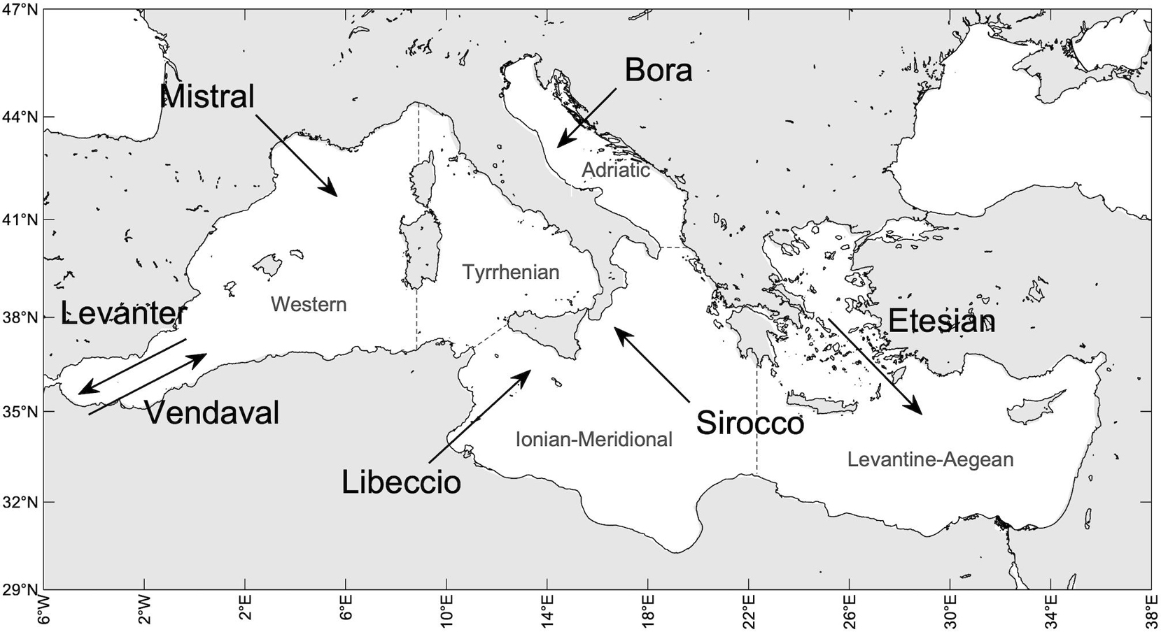
Figure 1. Map of the Mediterranean Sea basin and sub-basins (separated for the climate analysis purposes of this paper by dashed gray lines). The most relevant regional winds are indicated by black arrows denoting blow-to direction.

The purpose of this paper is to characterize the typical and extreme climate of the MS wind waves, together with its spatio-temporal variability and changes at a long-term spanning four decades (1981–2019). To cope with the requirements of such a complex environment and characterize the wave climate therein, we rely on a long-term and high-resolution wave hindcast, obtained by combining numerical wave modeling and atmospheric reanalysis. We have thus run the WAVEWATCH III model [Tolman, 1991; The WAVEWATCH III Development Group [WW3DG], 2019] with the ERA5 reanalysis wind forcing (Hersbach et al., 2018, 2020) and performed a wave climate analysis. In doing so, we do not expect to cover all aspects of the wave climatology of the MS, some of which have been addressed in various studies and publications (an non-exhaustive list of them can be found in Section “The study area”). We rather aim at bestowing new results based on state-of-the-art numerical modeling and reanalysis data, using one of the longest and most recent datasets to date. A novel season definition for the MS states based on observed data is proposed and adopted. Additionally, and most importantly, for the first time, we present and discuss the MS climate of expected maximum individual waves and of the most relevant factors for their development.

The paper is structured as follows. The study area, the wave hindcast and the methodology we have used for the wave climate analysis are detailed in Section “Methodology and Data”. In Section “Results” we present the results of this wave climate analysis, which first focuses on the significant wave height of sea states, showing its typical and extreme seasonal climate in the MS, its spatio-temporal variability and change, and then on the expected maximum individual waves and relevant parameters for their estimation (wave steepness and narrow bandedness). Section “Discussion” is a discussion on the limits and strengths of this dataset and on the results of the wave climate analysis, also compared to previous studies in the same region. Conclusions in section “Conclusion” close the paper.

Methodology and Data

The Study Area

The MS is a mostly deep (1,500 m on average) semi-enclosed regional sea, connected to the west to the Atlantic Ocean by the narrow Gibraltar Strait and to the east to the Black Sea by the Bosporus and Gallipoli (Dardanelles) Straits. Geographically, it is located between the European and the African continents and, from a climatic perspective, at the transition between a midlatitude regime zone, to the north, and a subtropical regime zone, to the south. Meteorologically, the MS region is interested by an intense synoptic-scale activity, with a separate branch of the northern hemisphere storm track passing over the region (Lionello and Sanna, 2005). The MS has a complex morphology, with many islands and peninsulas dividing the basin into sub-basins, some of them connected by straits (Figure 1). Together with the presence of steep mountain ridges close to the coast, this morphological complexity provides to the MS environment with a spatial heterogeneity, which also reflects on the MS region meteorology and climate, making their successful modeling far from being trivial (Lionello, 2012). In addition, and most important for the topic of this study, the orographic complexity of the MS region plays a fundamental role in the genesis of cyclones. In this context, cyclones typically originate (mostly in the western MS) from the interaction of synoptic-scale flows with the mountains, constraining the flow in the lower troposphere and producing local and often strong winds (Lionello, 2012).

In general, the MS wind climate is characterized by the occurrence of winds with regional spatial structure (200–1,000 km) and seasonal variability (Zecchetto and De Biasio, 2007; Lionello, 2012). In Figure 1 we have indicated the most relevant winds for the different sub-basins. Levanter and Vendaval winds blow in the westernmost part of the MS (Western sub-basin), respectively, from the north-east and the south-west: the first during all seasons (but most intensely in winter), the second mainly during autumn and spring. Mistral is a cold dry wind jet, stronger during winter, blowing from the north/north-west over the western and Tyrrhenian sub-basins and occasionally reaching the African coasts. Libeccio and Sirocco are southerly winds blowing in the Tyrrhenian and Ionian-Meridional sub-basins: the first mainly in winter from the south-west, the second mainly in autumn and spring from the south-east. Sirocco is also channeled into the Adriatic sub-basin, and it contributes to the intense storm surges that take place in the northern Adriatic Sea and in the Venice lagoon (Cavaleri et al., 2019). The other dominant wind in the Adriatic climate is Bora, a cold and dry north-easterly wind producing jets over the sea after interacting with the local orography. Northerly winds also dominate the climate in the Levantine-Aegean sub-basin: Etesian winds blow the from north/north-west and are particularly strong during summer.

The climate of wind waves in the MS, mostly driven by these regional winds, is subject to the morphological complexity constraints described above, resulting in limited fetches in large parts of the basin (with some exceptions) and in coastal shallow regions relatively proximal to the generation areas. Some regions present peculiar characteristics, for instance the northern Adriatic Sea or the Aegean Sea, where wave propagation experiences either the evolution over a relatively shallow flat bottom or the shadowing by numerous islands, respectively. Most of the studies on the MS wave climate (including a wind and wave atlas of the MS, Western European Union and Western European Armaments Organisation Research Cell, 2004) based on hindcast or observed data, focused on the extreme significant wave height (e.g., the monthly 99th percentile: Sartini et al., 2015a; Sartini et al., 2015b, 2017; De Leo et al., 2020; Morales-Márquez et al., 2020) with only a few exceptions that focused on the average significant wave height (for instance, Lionello and Sanna, 2005; De Leo et al., 2020). Others were dedicated to the assessment of the wave energy climate at specific locations or over the whole basin, with energy harvesting purposes (Barbariol et al., 2013; Liberti et al., 2013; Arena et al., 2015; Besio et al., 2016). A similar approach to the one presented in this paper, although with a different purpose, can be found in von Schukmann et al. (2021), where Benetazzo et al. have used a shorter portion of our dataset for an assessment of the climate of the maximum individual waves in the MS in the last quarter of a century, focusing on the 2019 anomalies and their physical interpretation. The complexity of the MS climate has also been exploited to test novel approaches for wave climate analysis (Sartini et al., 2015b; Portilla-Yandún et al., 2019). Besides providing the statistics over decadal periods (generally one to three decades), some of the previous studies used statistical and data analysis approaches to obtain accurate return level estimates of the significant wave height (e.g., Sartini et al., 2015a), and to describe the spatio-temporal variability and the long-term change (trends) of the wave climate (e.g., Sartini et al., 2017; De Leo et al., 2020; Morales-Márquez et al., 2020). To interpret inter-annual and inter-decadal variabilities, some studies also tried to relate them to the modes of atmospheric variability, looking for teleconnection patterns and using climate indices (Lionello and Sanna, 2005; Morales-Márquez et al., 2020). Finally, some studies were devoted to providing projections of the future wave climate under climate change scenarios over the whole basin or sub-basins (see for instance, Benetazzo et al., 2012; De Leo et al., 2021).

Mediterranean Sea Waves Hindcast

Wave Model Setup

The climate of MS wind waves, its spatio-temporal variability and change presented in this paper are grounded on a numerical model hindcast, produced by running the wave model WAVEWATCH III^® (hereinafter WW3; version 6.07;¹) for a 40-year long period from 1980 to 2019 over the whole MS basin (Figure 1). WW3 is a third-generation spectral wind-wave model that solves the random-phase spectral action density balance equation for wavenumber-direction spectra [Tolman, 1991; The WAVEWATCH III Development Group [WW3DG], 2019]. Various source-term packages allow computing wave generation by wind, decay by dissipative processes, nonlinear wave-wave interactions, and wave transformation near the coast. For this study, WW3 has been run over a high-resolution structured curvilinear grid with a horizontal spacing of 0.05° (∼5 km). WW3 has been forced with the 10-meter wind speed horizontal components (u₁₀,v₁₀) provided hourly by the ERA5 atmospheric reanalysis, over a 0.25° resolution horizontal structured grid (Hersbach et al., 2018). To represent wave growth and decay in WW3, we have used the state-of-the-art ST4 source-term parameterization of Ardhuin et al. (2010), relying on the default values, but adjusting some coefficients in agreement with the results of TEST405 of the Ardhuin et al. study [The WAVEWATCH III Development Group [WW3DG], 2019] to values that are supposed to perform well for younger seas (β_max = 1.55 and z_0,max = 0.002). Wave propagation has been computed using a third-order accurate scheme, together with the discrete interaction approximations for nonlinear wave-wave interactions, and accounting for subgrid-scale obstructions (propagation-based approach; Tolman, 2003), very common in some parts of the MS (e.g., Adriatic and Aegean seas). In shallow waters (i.e., coastal areas and the northern Adriatic Sea) bottom friction has been modeled using the JONSWAP parameterization with default values (Hasselmann et al., 1973), while the depth-induced wave breaking has been parametrized following Battjes and Janssen (1978). To define the bottom topography and coastlines we have used the ETOPO1 relief model (doi: 10.7289/V5C8276M).

Wave Model Outputs

The model outputs considered in this study, produced at hourly rate, are the significant wave height H_s, the maximum expected crest height ${\overline{C}}_{\text{max}}$, and the maximum expected crest-to-trough height ${\overline{H}}_{\text{max}}$. Results for H_s and ${\overline{H}}_{\text{max}}$ are presented in the paper, while results for ${\overline{C}}_{\text{max}}$ are in the Supplementary Material. The maximum individual crest and crest-to-trough heights herein considered are computed using the space-time extreme WW3 model implementation distributed since version 5.16 [The WAVEWATCH III Development Group [WW3DG], 2016] which assumes nonlinear (for ${\overline{C}}_{\text{max}}$) and linear (for ${\overline{H}}_{\text{max}}$) constructive interference of directionally spread waves as the leading mechanism for the generation of the largest waves in a sea state. In particular, the WW3 implementation is based on the Tayfun (1980) approximation of the second-order nonlinear model for ${\overline{C}}_{\text{max}}$ and on the linear Quasi-Determinism model for ${\overline{H}}_{\text{max}}$ (Benetazzo et al., 2017), such as they can be defined over a given space-time domain as:

$$\begin{array}{c}{\overline{C}}_{\text{max}}=\left({\xi }_0+\frac{\mu }{2}\frac{{\xi }_0^2}{\sigma }\right)\hfill \\ +\sigma \gamma \left[(1+\mu {\xi }_0{\sigma }^{-1}){\left({\xi }_0{\sigma }^{-1}-\frac{2N_3{\xi }_0{\sigma }^{-1}+N_2}{N_3{\xi }_0^2{\sigma }^{-2}+N_2{\xi }_0{\sigma }^{-1}+N_1}\right)}^{-1}\right]\hfill \end{array}(1)$$

$$\begin{array}{c}{\overline{H}}_{\text{max}}=\left[{\xi }_0+\sigma \gamma {\left({\xi }_0{\sigma }^{-1}-\frac{2N_3{\xi }_0{\sigma }^{-1}+N_2}{N_3{\xi }_0^2{\sigma }^{-2}+N_2{\xi }_0{\sigma }^{-1}+N_1}\right)}^{-1}\right]\hfill \\ \sqrt{2(1+|{\psi }^{*}|)}\hfill \end{array}(2)$$

In Equations (1) and (2), ξ₀ is the mode of the probability density function of linear space-time extremes (Fedele, 2012), σ = H_s/4 is the standard deviation of sea surface elevation, N₃, N₂ and N₁ are the average numbers of waves in the space-time domain and over its boundaries (Benetazzo et al., 2017), γ = 0.5772 is the Euler-Mascheroni constant, μ is the wave steepness and ψ^∗ is the narrow bandedness parameter. Steepness and bandwidth are sea state characteristics that contribute to the maximum individual wave height characterization. ψ^∗ is defined as the absolute value of the first minimum of the autocovariance function of the sea state (Boccotti, 2000). As both μ and ψ^∗ are not direct outputs of WW3, we have a posteriori derived them, as $\mu =H_s/(g{T}_m^2/2\mathrm{\pi })$, with T_m being the mean zero-crossing spectral wave period produced by WW3, and from ${\overline{H}}_{\text{max}}={\overline{C}}_{\max ,1}\sqrt{2(1+{\psi }^{*})}$ (Boccotti, 2000) by deriving the linear estimate of the maximum expected crest height ${\overline{C}}_{\max ,1}$ from ${\overline{C}}_{\text{max}}$, using the Tayfun (1980) quadratic equation [Equation (36) of Benetazzo et al., 2017]. Further details on the space-time extreme theoretical framework implemented in WW3 can be found in Barbariol et al. (2017); Benetazzo et al. (2021b) and references therein. A discussion on the role of wave steepness and bandwidth on the maximum individual wave heights during extreme events is given by Benetazzo et al. (2021a).

Our climatology of maximum individual waves deals with the maximum crest height ${\overline{C}}_{max}$ and the maximum crest-to-trough height ${\overline{H}}_{max}$ that might be expected in 20-min sea states and over a 100 m × 100 m area. This duration and spatial extent point to a customary sea state duration [e.g., measured by in situ instruments as a buoy, World Meterological Organization [WMO], 2018] and to the horizontal sea surface area covered by an offshore structure (e.g., a large oil/drilling rig), respectively.

Assessment Methodology

The MS wind-wave hindcast has been assessed using satellite altimeter observations of H_s, starting from 1991. Altimeter H_s data have been retrieved from the IMOS platform² (Ribal and Young, 2019; Young and Ribal, 2019), which provides calibrated and cross-validated data (we have only retained data flagged as “good data,” which according to the authors of those studies proved very reliable). Satellite missions considered in the August 1991–December 2019 period, for a total of 4066142 collocations, are listed in Supplementary Table 1. The longest dataset is 14-year long (ERS-2), the shortest is almost 4-year long (SENTINEL-3A). To inter-compare modeled and observed data for validation purposes, wave hindcast data have been bi-linearly interpolated in space and linearly interpolation in time on the satellite data points location and time. The statistical parameters and error metrics used to evaluate the hindcast performance are the model-observation bias $BIAS={\overline{H}}_{s,WW3}-{\overline{H}}_{s,altimeter}$ (overbar denoting ensemble average), the relative bias $RBIAS=({\overline{H}}_{s,WW3}/{\overline{H}}_{s,altimeter}-1)\times 100$, the Pearson cross-correlation coefficient CC, the Mean Absolute Error $MAE=\overline{|H_{s,WW3}-H_{s,altimeter}|}$ and the slope of the best-fit line (linear regression).

To assess that the ERA5 climatological signal transferred from the surface wind to waves can represent the intra- and inter-annual climatological variability of MS waves, as well as the trends, we have estimated the correlation between the monthly 50th and 99th percentile H_s from satellite altimeters and co-located WW3 hindcast and compared the linear trends of observed and modeled data. For these specific latter tasks, we have retained only satellite datasets longer than 10-year (see Supplementary Table 1).

Modeled maximum individual waves are generally verified at the short-term (i.e., sea state) time scale (see e.g., Barbariol et al., 2017, 2019; Benetazzo et al., 2021a, b), as there are no observational platforms in the global oceans that are continuously collecting this type of data over a long-term period. In addition, the model-to-observation comparison would require using observations with the same space and time domain sizes used for the hindcast (i.e., 20 min and 100 m × 100 m), while the sizes used for observations (application dependent and fixed) may be different from those required. Hence, the assessment of the WW3 hindcast in terms of ${\overline{C}}_{max}$ and ${\overline{H}}_{max}$ can be only done indirectly. We rely here on the assessment of H_s, which is the pivotal parameter for determining the height of maximum expected individual crest and crest-to-trough heights (Benetazzo et al., 2021b).

Wave Climate Analysis

The climatology of wind-wave sea states in the MS is presented by using the 50th (i.e., median) and the 99th percentiles of the significant wave height H_s, which may represent typical and extreme sea-state conditions, respectively. Similarly, the climatology of maximum individual waves is based on the 50th and 99th percentiles of the maximum crest-to-trough height ${\overline{H}}_{\text{max}}$ (and maximum crest height ${\overline{C}}_{\text{max}}$ in the Supplementary Material).

In order to highlight the effects of intra-annual variability, the 50th and 99th percentiles are estimated at seasonal scale and averaged over the length of the hindcast to provide an empirical estimate of the expected typical and extreme conditions during the different seasons. In this study, we propose and adopt a novel definition of stormy seasons for the MS wind-wave climate based on the observed H_s data in the MS, rather than using the canonical meteorological definition based on the air temperature (i.e., winter: December, January, February, DJF; spring: March, April, May, MAM; summer: June, July, August; JJA; autumn: September, October, November, SON). To this end, satellite altimeter observations of H_s are used (see Section “Assessment Methodology”). Yearly-averaged monthly H_s values are first computed for each satellite altimeter and then the eight satellites are combined to obtain the ensemble average and standard deviation.

To let the interannual climate variability and climate change due to external forcings emerge, we remove the source of intrinsic intra-annual variability due to seasonality by taking separately into account the different seasons, as done for instance by Morales-Márquez et al. (2020). Therefore, in the result presentation (climate variability and climate change), we shall focus on the two most representative seasons only, i.e., winter and summer. The interannual climate variability is shown in terms of climate anomalies, which are defined as deviations of the winter and summer 50th and 99th percentile values of a generic wave height H in a specific i^th year $H_i^{pp}$ (pp = 50, 99) with respect to the winter and summer yearly-averaged 50th and 99th percentiles ${\overline{H}}^{pp}$ (overbar denoting average over the years), i.e., $H_i^{pp}-{\overline{H}}^{pp}$. Further, to assess the spatial distribution of the inter-annual climate variability and highlight the MS sub-basins and regions that have experienced the largest variations in the study period, we have also normalized anomalies with respect to the local yearly averages, thus showing the relative anomalies, i.e., $(H_i^{pp}-{\overline{H}}^{pp})/{\overline{H}}^{pp}$. In order to motivate the inter-annual climate variability of the MS waves, we look for possible teleconnections between the wave climate variability and the principal modes of atmospheric variability, taking into account four northern hemisphere indices (downloaded as monthly averaged values from³): North Atlantic Oscillation (NAO), Scandinavian (SCAND), East Atlantic (EA) and East Atlantic-Western Russian (EAWR). Monthly mean data are then combined to obtain seasonal averages.

Finally, in order to assess any potential long-term change in the typical and extreme sea state climate over 1981–2019, the linear trend of winter and summer $H_s,{\overline{C}}_{\text{max}}$ and ${\overline{H}}_{\text{max}}$ are estimated over the whole MS and sub-basins through the Sen’s slope of the 50th and 99th percentiles (Theil, 1950; Sen, 1968), testing the statistical significance at the 90% confidence interval with the Mann–Kendall test (Mann, 1945; Kendall, 1948).

Results

The characteristics of the MS wind-wave climate obtained from the ERA5 wind forced WW3 hindcast are presented in this Section stemming from the yearly-averaged seasonal 50th and 99th percentiles of H_s (the conventional variable used to describe the wave climate), together with their variability and change. Same analyses are also conducted to investigate the distribution of the crest-to-trough height of the maximum individual waves ${\overline{H}}_{\text{max}}$ (results for the crest height of the maximum individual waves ${\overline{C}}_{\text{max}}$ are in the Supplementary Material). Before presenting the MS wind-wave climatology a novel definition of seasons for the MS states and the assessment of the wave hindcast performance are introduced.

An Observed Data-Based Definition of Seasons for the Mediterranean Sea States

The monthly 50th and 99th percentiles of H_s, as observed over the MS by the eight satellite altimeters used for the hindcast assessment (Supplementary Table 1) are shown in Figure 2A. Observations are also normalized with respect to the maximum monthly H_s percentile (Figure 2B), which occurs in January for both the 50th and 99th percentiles. Both typical and extreme sea states clearly show two dominant regimes: a stormy period, from November to March (with values within 20% of the January H_s; Figure 2B), and a relatively calm period, from June to August (with values within few per cent of the minimum H_s, occurring in June for the 50th percentile and in August for the 99th percentile). In between, there are two transitional seasons. Following this variability, we define the four sea-state “seasons” as winter (NDJFM), spring (AM), summer (JJA) and autumn (SO). Compared to the classic meteorological definition, we therefore propose a longer winter season, starting in November and ending in March (both showing significantly larger H_s compared to the other spring and autumn months), and shorter transitional seasons (2-month long), with summer remaining unchanged. This definition applies to the whole basin but still holds if only northern, southern or western sub-basins are considered. If only the eastern part of MS is accounted for, the relative difference between summer and transitional seasons reduces (not shown here), most likely due to the effect of Etesian wind-waves. This is in agreement with findings of Queffeulou and Bentamy (2007) who pointed out differences in western to eastern MS monthly mean H_s from satellite altimetry, especially during summer season. November and December H_s values clearly belong to the winter season that accounts for the early months of the following year; therefore, to have an equal number of seasons, we start counting seasons from winter 1981 (beginning with November 1980) to autumn 2019 (ending in October 2019), thus analyzing only 39 years in the whole period (hereinafter 1981–2019).

FIGURE 2

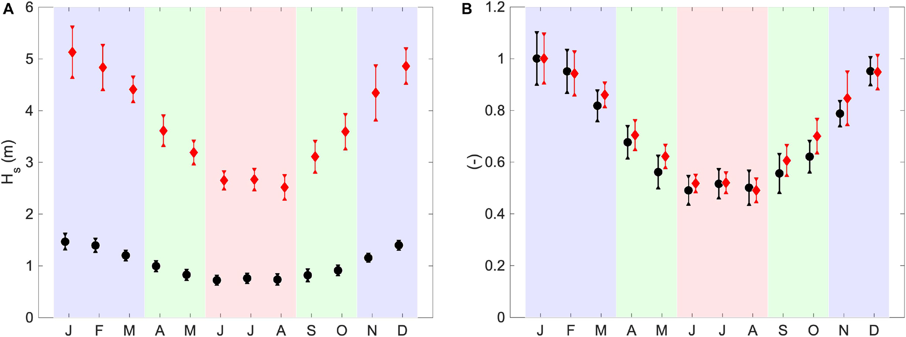
Figure 2. Yearly-averaged monthly 50th (black dots) and 99th (red diamonds) percentiles of H_s over the MS, from eight satellite altimeters (see Supplementary Table 1), dimensional [panel (A)] and normalized with the maximum value [panel (B)]. Dots and diamonds represent the ensemble average over the altimeter percentiles and bars represent the confidence intervals over the altimeter percentiles (± an ensemble standard deviation). Violet shading indicates winter months (NDJFM), red shading summer months (JJA) and green shading spring and autumn (transitional seasons; AM and SO).

Assessment of the Mediterranean Ses Wind-Wave Hindcast

The MS wind-wave hindcast performance in the 1991–2019 period against satellite altimeter observations is summarized in Figure 3, which collects information about the relative model-observation bias RBIAS in the MS and in the sub-basins (Figure 3A), the H_s scatter (Figure 3B) and the relation between modeled and observed climate variability and change (Figures 3C,D). Modeled H_s is simulated in the MS with 0.87 best-fit line slope, BIAS = −0.12 m and MAE = 0.26 m. The relative model-observation bias at the 50th percentile of modeled H_s (0.93 m; blue dot in the Figure 3B) is −8%, while at the 99th percentile (3.78 m; red dot in the Figure 3B) it is −14%, denoting a decrease in model performance with H_s, in agreement with the MS wave hindcast study of Mentaschi et al. (2015; verified against in situ wave buoys). The model-observed bias might be partially corrected by calibrating the input/dissipation source term parameterization in WW3. However, the spatial heterogeneity of the MS (with narrow, semi-enclosed sub-basins or/and surrounding orography) makes it difficult to achieve a set of parameters that is optimized to obtain good performance in the whole MS basin and in the whole H_s range (Lionello and Sanna, 2005; Mentaschi et al., 2015; Sartini et al., 2017; Morales-Márquez et al., 2020). This can be seen by comparing the slope of best-fit lines and the relative bias at different percentiles for the MS with those for the sub-basins. Best performance is achieved in the widest sub-basins (Ionian, Levantine), with larger slope and smaller relative bias compared to those obtained in the whole MS. Worst performance are in the Adriatic Sea, where the ERA5 wind is less effective in correctly reproducing wind and then waves due to spatial resolution effects in a narrow basin. These effects are partially visible also in the Tyrrhenian and Western sub-basins (both with islands and narrow parts), although performance in these sub-basins is comparable to that for the MS.

FIGURE 3

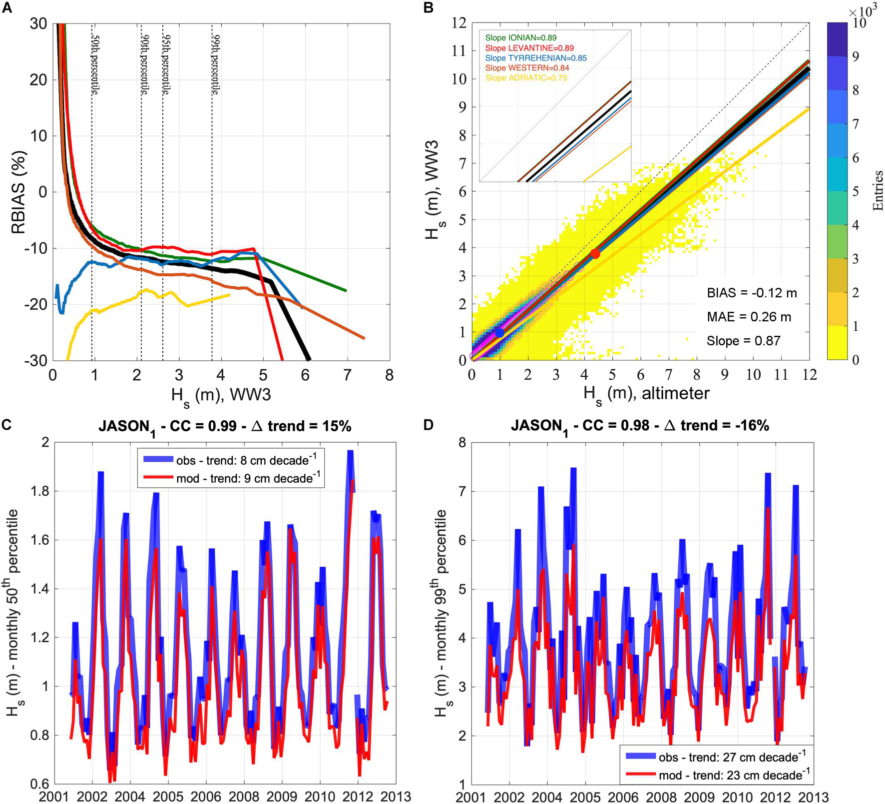
Figure 3. Performance of the WW3 wave hindcast in the MS and sub-basins against satellite altimetry (missions in Supplementary Table 1), August 1991–December 2019. [panel (A)] Relative H_s bias RBIAS as a function of H_s,WW3, with relevant percentile levels for the MS relative bias indicated by dashed lines. Black line: MS; green line: Ionian; red line: Levantine; blue line: Tyrrhenian; orange line: Western; yellow line: Adriatic. [panel (B)] Scatter plot and statistics for the MS. Purple circles are the Q-Q plot, with the blue dot denoting the 50th percentile and the red dot the 99th percentile. [panel (C)] Observed (JASON-1) and modeled (WW3) monthly 50th percentiles of H_s over the MS. Correlation coefficients (CC) and relative model-observation difference in trends are indicated in title. [panel (D)] Observed (JASON-1) and modeled (WW3) monthly 99th percentiles of H_s over the MS. Panel description as in panel (C).

The average (and standard deviation of) correlation coefficients between the monthly 50th and 99th percentile H_s from satellite altimeters and co-located WW3 hindcast are: 0.98 ± 0.004 for the 50th percentile and 0.97 ± 0.009 for the 99th percentile. An example of the monthly percentiles time-series for JASON-1 is shown in Figures 3C,D, with correlation coefficients larger than or equal to 0.98 for both 50th and 99th percentiles. Also, the linear trends of H_s estimated from the same satellite altimeters and co-located model data are in agreement, with consistent (i.e., both positive or both negative) Sen’s slope signs and a general tendency for larger model trends for the 50th percentiles and smaller for the 99th percentiles (compared to JASON-1, the relative trend differences are 15 and −16% for the 50th and 99th percentile, respectively, while the largest relative difference is −43%, between Envisat and model 99th percentile H_s trends).

Mediterranean Sea Wind-Wave Climate

The yearly-averaged seasonal 50th percentile of H_s is shown in Figure 4. As expected, the largest values occur during the winter (NDJFM) season when wind speeds are typically stronger (Zecchetto and De Biasio, 2007). Spatial patterns of the 50th percentile H_s are rather different in winter and summer (JJA), on the one hand, and very similar in spring (AM) and autumn (SO), on the other hand. The most energetic sea states occur over the western and southern sub-basins in winter (50th percentile up to 1.5 m) and spring (up to about 1 m), and over the eastern and western sub-basins in summer (up to 1.25 m) and autumn (up to 1.0 m). The western basin experiences the largest typical conditions over all seasons except summer, particularly the Sardinian Sea (amid the Gulf of Lyon, Sardinia, the North African coast and the Balearic Islands) where the north-westerly Mistral wind persistently blows from the French inland (Zecchetto and De Biasio, 2007). In summer, the largest wave heights are attained in the Aegean and Levantine basins (particularly southeast of Crete, with a typical jet-like pattern) with values comparable to those of winter and produced by the north-westerly Etesian winds, typical of late spring, summer and autumn seasons but reaching their maximum intensity during summer (Zecchetto and De Biasio, 2007).

FIGURE 4

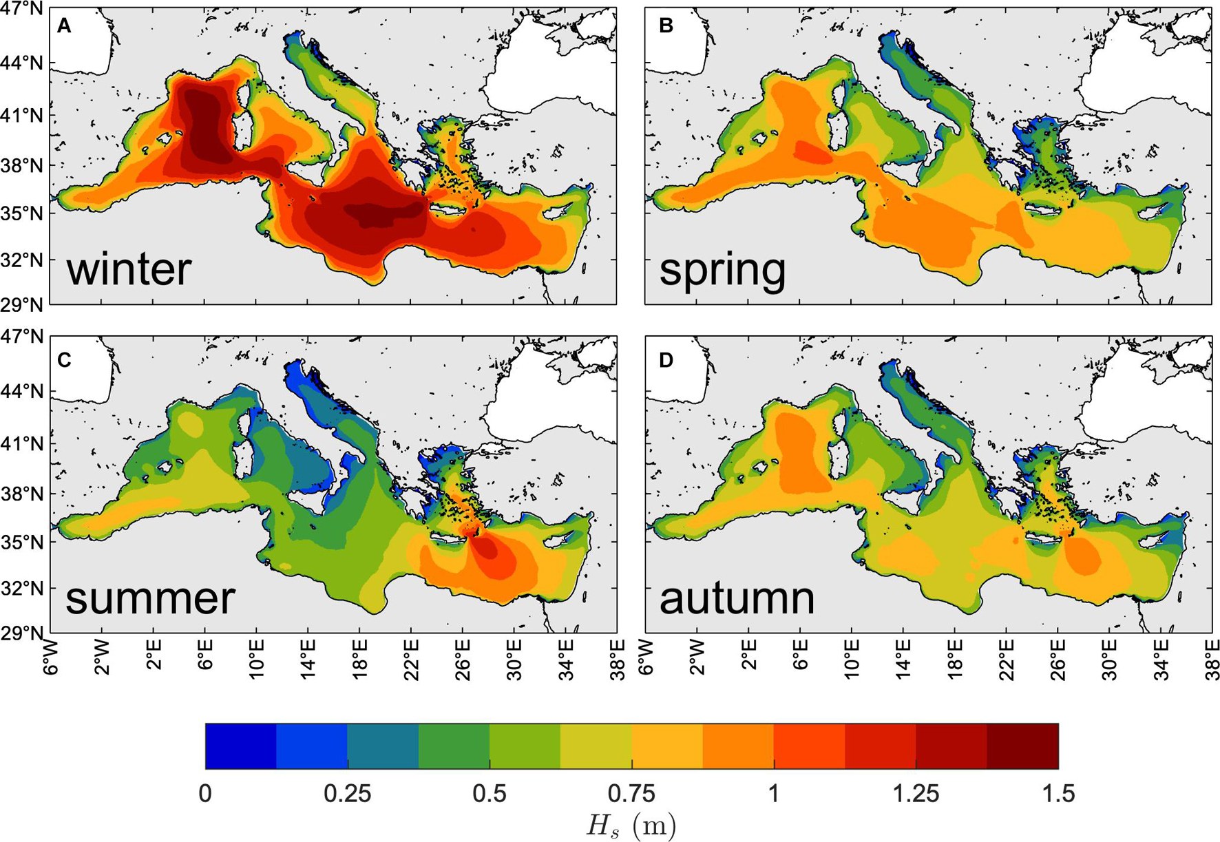
Figure 4. Climate of typical MS wind waves. Yearly-averaged seasonal 50th percentile of H_s (1981–2019): winter [NDJFM, panel (A)], spring [AM, panel (B)], summer [JJA, panel (C)], and autumn [SO, panel (D)].

The yearly-averaged seasonal 99th percentile of H_s is shown in Figure 5. The spatial distribution of extreme sea states is different compared to that of typical conditions (Figure 4). Indeed, the 99th percentile of H_s in all seasons have similar spatial patterns, and in particular the sea severities during spring and autumn seem comparable (despite some minor differences, for instance in the Alboran Sea and the Levantine basin). The largest values occur in the Gulf of Lyon and Sardinian Sea (up to 5.5 m in winter, up to 4.0 m in summer, up to 4.5 m in spring and autumn). Other regions with large, though smaller, values are located in the southern (Ionian Sea) and eastern (Levantine Sea) sub-basins, while the summer waves southeast of Crete island (the largest in the summer 50th percentile maps; jet-like pattern) are surpassed by the extreme waves generated by the Mistral wind in the Gulf of Lyon. In the Adriatic Sea, the spatial pattern changes compared to the 50th percentile, with large values more homogeneously distributed over the whole basin (including in the northern part) and with the largest ones (in the southern part) off the eastern coast, as a consequence of the south-easterly Sirocco wind storms hitting the Croatia, Albany and Montenegro shorelines.

FIGURE 5

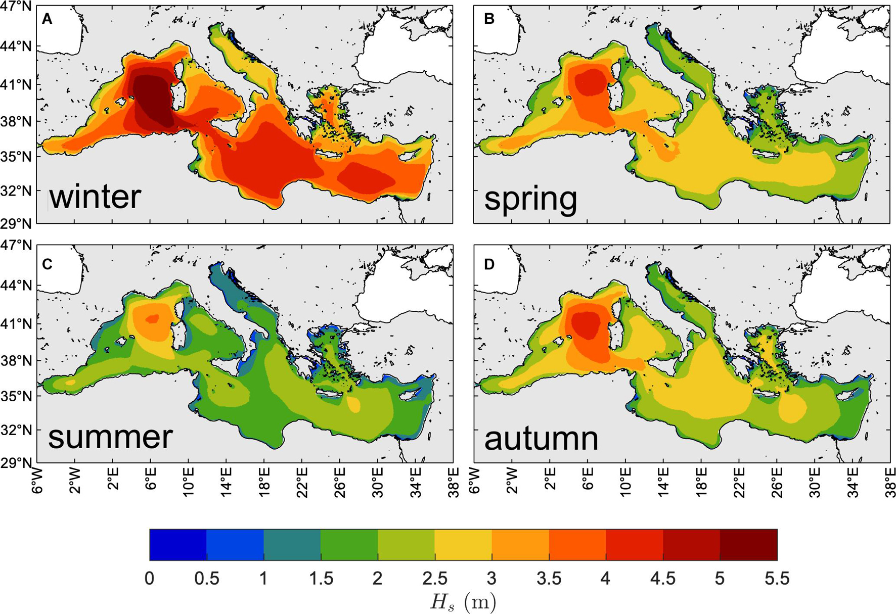
Figure 5. Climate of extreme MS wind waves. Yearly-averaged seasonal 99th percentile of H_s (1981–2019): winter [NDJFM, panel (A)], spring [AM, panel (B)], summer [JJA, panel (C)], and autumn [SO, panel (D)].

Variability of the Mediterranean Sea Wind-Wave Climate

The first assessment of the wave climate variability is made by analyzing the intra-seasonal extreme-to-typical condition variations. In Figure 6 we show the winter (NDJFM) and summer (JJA) ratios 99_p,Hs/50_p,Hs of the 99th to the 50th percentile of H_s. This ratio provides a measure of the width of the empirical probability distribution of H_s at seasonal scale and it is yearly-averaged to obtain an empirical estimate of the expectation. We observe that sea states are much more variable during summer than winter, with the largest values of 99_p,Hs/50_p,Hs. There is also a larger spatial variability of the ratio during summer with respect to winter. Indeed, during winter extreme conditions are generally up to four times greater than the typical ones, over all the MS basin, with only spatially limited exceptions in the northern Adriatic, southern Tyrrhenian, western Aegean seas and eastern Levantine sub-basin, where they can be up to six times larger (locally, more than six times). During summer, extreme conditions can be more than six times larger than typical ones (up to eight times) over large parts of the central MS, including the Sardinian, Tyrrhenian and Adriatic Seas. The lowest summer variability occurs in the Levantine basin, where the sea states generated by the steady and low-variability Etesian winds are intense but constant over the season.

FIGURE 6

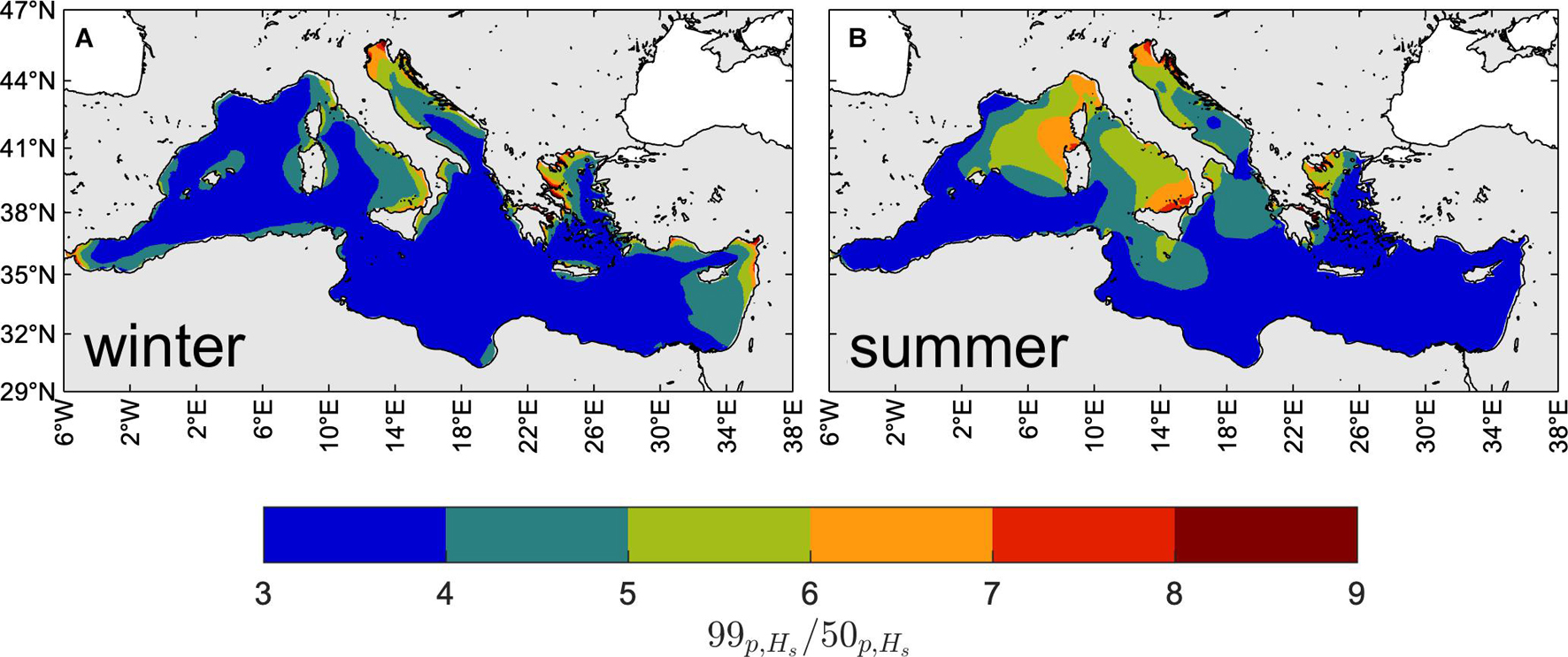
Figure 6. Intra-seasonal variability of the wind-wave climate. Yearly-averaged ratio of the 99th to 50th percentile of H_s (1981–2019), during winter [NDJFM, panel (A)] and summer [JJA, panel (B)].

We now proceed by assessing the interannual variability of the wave climate in the MS region by showing the standard deviation and range of the anomalies of typical and extreme H_s during winter and summer. We first focus on the standard deviation of the H_s anomaly, which is used to point out the regions with the largest climate variability over the years. Then, we focus on the standard deviation and range (maximum-minus-minimum) of the relative anomaly (i.e., with respect to the yearly-averaged percentiles of H_s, see Section “Wave Climate Analysis” for the definition) to show the regions with the largest variability with respect to the local wind-wave climate (and quantify it), allowing to inter-compare regions with different H_s percentiles. The interannual variability of the 50th percentile of H_s is presented in Figure 7. During winter the largest variability occurs in the Western sub-basin (Mistral wind region, up to 0.25 m standard deviation; Figure 7A); in summer, in the Aegean and Levantine sub-basins (Etesian wind region, up to 0.2 m standard deviation; Figure 7D). These are also the regions with the largest 50th percentile of H_s (Figure 4) although the spatial distribution of the standard deviation of the H_s anomaly does not perfectly reflect that of the yearly-averaged 50th percentile of H_s. Looking at the standard deviation of the relative anomalies (Figures 7B,E), it emerges that the regions with the largest variability with respect to the local wave climate are in the Tyrrhenian, Adriatic and Aegean sub-basins during summer, and in the Western, Tyrrhenian, Adriatic, and Levantine sub-basins during winter. The maximum standard deviation of the relative H_s anomaly, up to 20% of the 50th percentile H_s in both summer and winter, occurs in the northern Adriatic Sea and the southern Tyrrhenian Sea, where during 1981–2019 winters the range of variability has reached 100% of the local 50th percentile H_s.

FIGURE 7

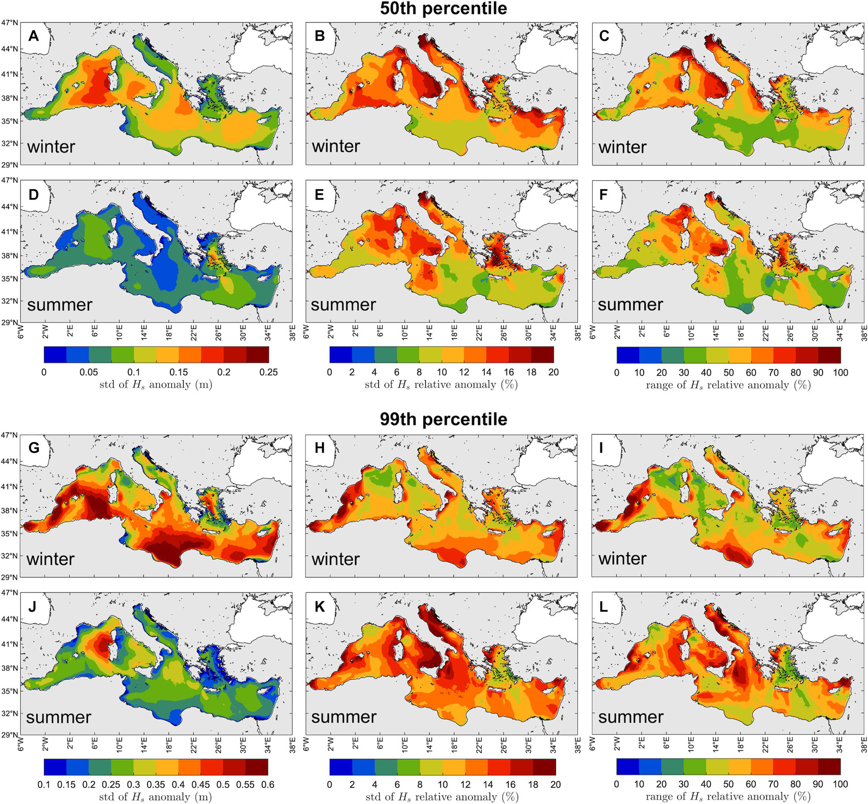
Figure 7. Inter-annual variability of the typical [50th percentile, panels (A–F)] and extreme [99th percentile, panels (G–L)] wind-wave climate. Standard deviation (std) of the H_s anomaly [panels (A,D,G,J)], standard deviation of the relative anomaly [panels (B,E,H,K)] and range [maximum-minus-minimum; panels (C,F,I,L)] of the relative anomaly of the winter (NDJFM) and summer (JJA) 50th and 99th percentile of H_S (1981–2019), with respect to the yearly-averaged winter and summer 50th (Figure 4) and 99th (Figure 5) percentile of H_S, respectively.

The interannual variability of the 99th percentile of H_s is presented in Figure 7, and show different characteristics with respect to that of the 50th percentile of H_s. Indeed, in summer the maximum standard deviation of the H_s anomaly is in the Western sub-basin (Sardinian Sea, 0.6 m; Figure 7J), where also the maximum 99th percentile occurs, whereas in winter the maximum standard deviation is in the southernmost (Ionian sub-basin, offshore Libya; Figure 7G) and westernmost (Western sub-basin, southeast and southwest of Balearic Islands) parts of the MS, which are not the locations with the maximum 99th percentile of H_s (Sardinian Sea and Gulf of Lyon, Figure 5). Similarly, the largest standard deviation of the relative anomaly (20% of the 99th percentile H_s) is in the Western, Tyrrhenian, Adriatic, Aegean and Ionian sub-basins during summer (as for the 50th percentile H_s; Figure 7K), while in winter the maximum is offshore Libya and southwest of the Balearic Islands (Figure 7H). In these regions, the range of the relative anomaly is up to the 100% of the local 99th percentile H_s.

To provide a synthetic description of the interannual climate variability at the regional scale (i.e., MS basin and sub-basins), in Figure 8 we show the time series of the spatially averaged relative anomaly of the 50th and 99th percentile of H_s over the MS (spatial averages over the sub-basins are shown in Supplementary Figures 1–5). In general, during 1981–2019 there is an alternation of positive and negative anomalies that, more frequently during winter and especially in some sub-basins, tend to aggregate forming clusters of years with (almost) only positive or negative anomalies. An example of this aggregation is the 1989–1994 anomaly of the winter 50th percentile H_s. During this period the largest negative anomaly in the MS have occurred (winter 1990, −18%), followed by four more seasons with negative, often considerable, anomalies. The largest negative anomaly at sub-basin scale have occurred in the Tyrrhenian Sea in the same period (winter 1989, −36% of the 50th percentile of H_s; Supplementary Figure 1), but similar pattern can be observed in the Ionian, Adriatic and Western sub-basins, even if with smaller anomalies. During 1989–1994 winters, the atmosphere in the MS region has been very stable, in particular over the Western, Tyrrhenian, Adriatic and Ionian sub-basins (Supplementary Figures 1–4; as shown in Supplementary Figure 6, displaying the 500 hPa geopotential height, sea level pressure and wind intensity anomalies over western Atlantic, Europe and western Asia from ERA5 atmospheric reanalysis, for some seasons of interest). The cause of this stability can be found in the localization of the pressure fields on a synoptic (European) scale (Supplementary Figure 6). The conditions that induce strong atmospheric stability over the MS basin have been marked positive 500 hPa geopotential anomalies and positive sea level pressure (SLP) anomalies over Europe, and negative wind intensity anomalies over the MS basin. Such conditions have occurred in all the 1989–1994 winters (as shown in Supplementary Figure 6 for 1989 and 1990), and are responsible for the negative H_s anomalies observed in Figure 8 for the MS and in Supplementary Figures 1–5 for sub-basins. The largest positive H_s anomaly in the MS (+21% of the 99th percentile of H_s) have occurred in winter 1981, while the largest positive anomaly at sub-basin scale occurred in the Tyrrhenian Sea in summer 2014 (+32% of the 50th percentile of H_s). Winter 1981 has been characterized by an average circulation over Europe (Supplementary Figure 6) with positive SLP anomaly over Western Europe, positive 500 hPa geopotential anomaly over Russia and a negative SLP anomaly on central and southern Europe and on Scandinavia. These conditions are associated with the meridional advection of arctic air and intense cyclogenesis over the MS, especially over the western part, as shown in Supplementary Figure 6 with maximum wind intensity anomalies of over 1.5 m/s on the Western and Ionian sub-basin (both showing very large positive extreme H_s anomalies in winter 1981, Supplementary Figures 3–4). Summer 2014 (Supplementary Figure 6) has been characterized by geopotential and SLP anomalies in the western MS, with the minimum pressure positioned on central-western Europe. This configuration generates frequent advections of relatively cold air along the eastern edge of the Azores anticyclone, producing positive wind intensity anomalies (with values between 0.5 and 1.5 m/s, Supplementary Figure 6) in the Western, Tyrrhenian and Adriatic sub-basins, all showing positive H_s anomalies in summer 2014. The temporal climate variability of typical H_s in the MS has been the largest in winter typical sea states as shown by the 8.62% standard deviation. At sub-basin scale the largest temporal variability of typical H_s has occurred in the Tyrrhenian, Adriatic and Western sub-basins, both in summer and winter (for the Tyrrhenian Sea, 11.3 and 13.6% standard deviation, respectively; see Supplementary Figure 1), in agreement with results about typical climate variability in Figure 7. Extreme H_s appears to be most variable in the Tyrrhenian and Adriatic seas during summer, and in the Ionian and Levantine sub-basins during winter, (for the Adriatic Sea summer 11.2% and for the Ionian Sea winter 8.9% standard deviation, respectively; see Supplementary Figures 2, 4), in agreement with results for the climate variability shown in Figure 7.

FIGURE 8

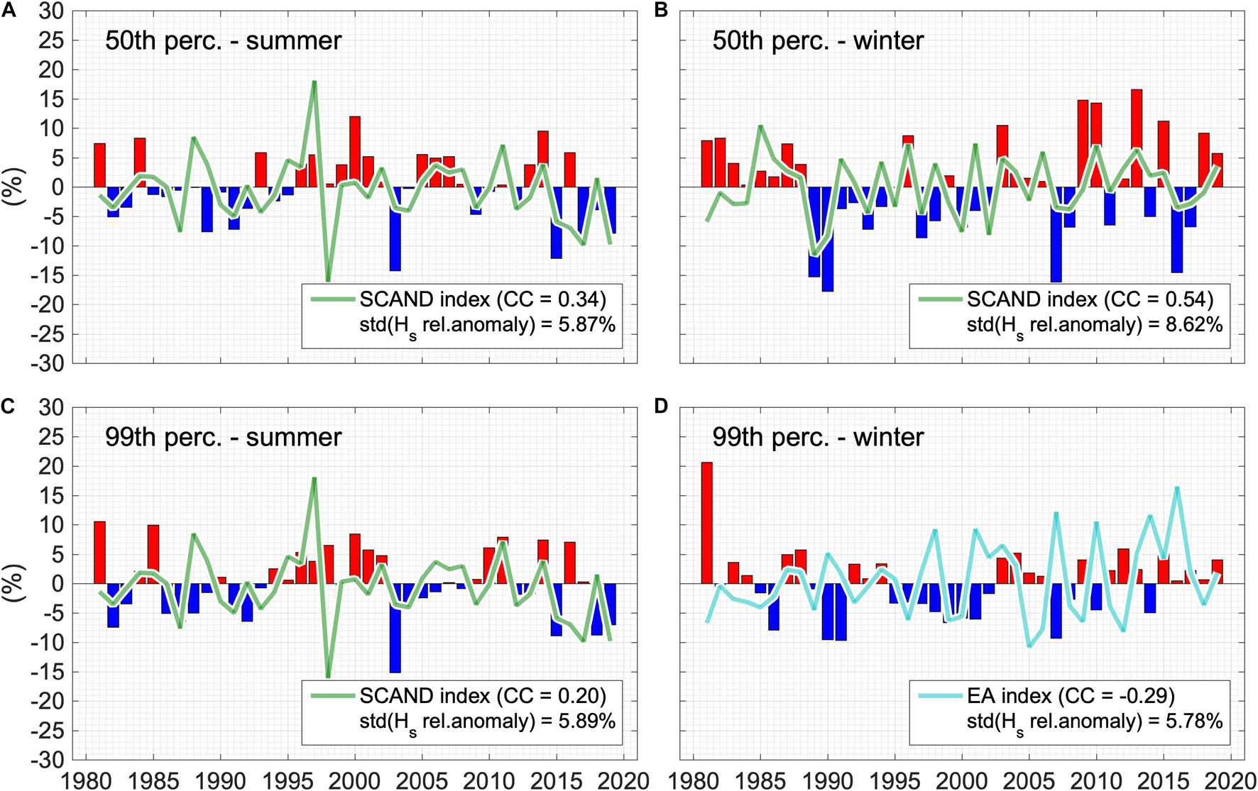
Figure 8. Inter-annual variability of typical and extreme wind-wave climate in the MS (1981–2019). Relative anomaly of 50th [panels (A,B)] and 99th [panels (C,D)] percentiles of H_s during winter and summer seasons, spatially averaged over the MS. Solid lines represent the most correlated teleconnection indices among NAO, EA, EAWR, and SCAND (correlation coefficient CC in the legend; indices are magnified ten times for graphical purposes).

The inter-annual climate variability of the MS waves observed inFigure 8 (and Supplementary Figures 1–5 for sub-basins) can be partially explained by possible teleconnections between the wave signals and the principal modes of atmospheric variability. To this end, we compare the time series of the relative anomaly with the time series of the NAO, SCAND, EA and EAWR indices. Thus, we have (i) averaged the monthly values of 1981–2019 indices over the winter and summer seasons, respectively, (ii) computed cross-correlation coefficients between the four indices and the MS (and sub-basins) H_s relative anomalies and then (iii) plotted in Figure 8 (and Supplementary Figures 1–5 for sub-basins) the time series of the index showing the highest correlation (in search for teleconnection). Generally, with only a few exceptions, relative anomalies in the MS and sub-basins are mostly correlated to SCAND positive phases, particularly, but not only, for the 50th percentiles. In the MS, this is observed for winter and summer typical and extreme sea states, except for winter extreme H_s, which is related to the EA negative phases. The highest correlations are found for the winter 50th percentiles, although the correlation coefficients are generally small, reaching 0.54 at most for the MS (SCAND and winter 50th percentile, Figure 8) and 0.65 maximum value for the sub-basins (SCAND and Tyrrhenian Sea winter 50th percentile, Supplementary Figure 1). The impact of the SCAND index on the Mediterranean atmosphere dynamics and hence on the MS wave climate can be observed, as an example, in the winter 1989 and 1990 atmospheric configuration (Supplementary Figure 6). The persistent low 500 hPa geopotential height and SLP fields over Scandinavia and Eastern Europe (with −1.2 and −0.8 seasonal SCAND index, respectively; Figure 8), induce negative anomalies of wind speed over the whole MS, which, in turn, generate negative anomalies of the 50th percentile H_s (−15 and −18%, Figure 8).

Change of the Mediterranean Sea Wind-Wave Climate

We assess here what might have been the climate change of the winter and summer MS sea states over 1981–2019 showing the maps of the H_s linear trends (using the Sen’s slope, in cm decade^–1, evaluated on 39 yearly data) in Figure 9 and their spatial averages over the basin and sub-basins in Table 1. We show both the trends at the points where there is statistically significance (at 90% confidence interval according to the Mann–Kendall test) and at all the points in a (sub-) basin, including where there is no statistical significance.

FIGURE 9

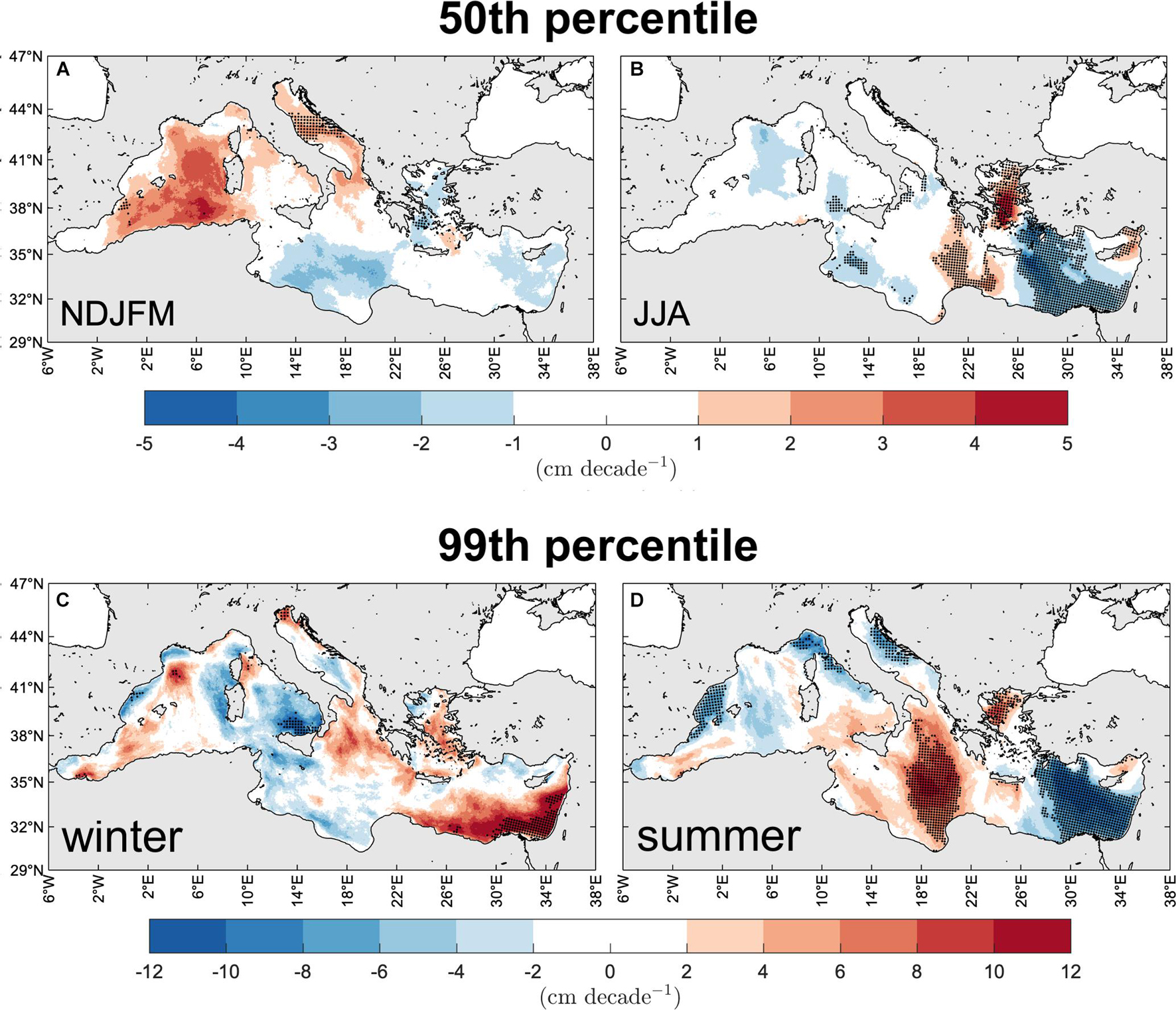
Figure 9. Change of the MS typical [50th percentile, panels (A,B)] and extreme [99th percentile, panels (C,D)] wind-wave climate. Trend of winter [panels (A,C)] and summer [panels (B,D)] H_s during 1981–2019. Area with statistically significant trends at the 90% confidence intervals are denoted by black dots (decimated for graphical purposes).

TABLE 1

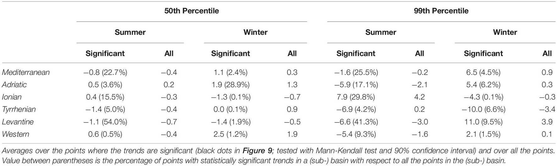
Table 1. Spatial averages over the MS and sub-basins of the 50th and 99th percentile H_s trends shown in Figure 9 (cm decade^–1), during 1981–2019 summer and winter seasons.

The winter 50th percentile of H_s (Figure 9A and Table 1) shows positive trends over large part of the western and northern sub-basins of the MS, and negative or no trends in the eastern and southern sub-basins, resulting in a substantially net zero trend for the MS typical winter sea states (0.3 cm decade^–1; Table 1). The largest increases are in the Sardinian Sea and offshore Algerian coasts (up to 5 cm decade^–1) and largest decreases in the southern MS (down to −3 cm decade^–1). However, only trends offshore the Algerian coasts, in the central Adriatic Sea (Sirocco and middle Bora jets regions) and in small portions of the Aegean and Balearic seas are statistically significant, bringing the spatial average to 1.1 cm decade^–1 (Table 1). The summer map (Figure 9B) is far different, showing generally smaller Sen’s slopes, except in some limited areas in the eastern part of the basin, with statistically significant increases (up to 4 cm decade^–1) in the Aegean Sea and eastern and western Levantine basin and decreases (down to −4 cm decade^–1) in the central Levantine basin where the summer Etesian winds blow. As a whole, the MS presents a very mild decreasing trend during typical summer sea states (−0.8 cm decade^–1; Table 1).

The 99th percentile H_strends, shown in Figures 9C,D, are significantly larger than the 50th percentile trends shown above. During winter the largest statistically significant changes are in the southern Levantine sub-basin with increases up to 12 cm decade^–1 offshore Egypt and Israel (11.0 cm decade^–1 on average in the sub-basin), in the Gulf of Lyon with increases up to 12 cm decade^–1 (Mistral jet region, despite a smaller average trend in the Western sub-basin), in the northern Adriatic Sea (northern Bora jet, increases up to 8 cm decade^–1) and in the southern Tyrrhenian Sea, the only statistically significant area of negative trend for winter extreme sea states (down to −12 cm decade^–1, −10.0 cm decade^–1 on average in the Tyrrhenian Sea). In the MS the winter 99th percentile H_s has increased 6.5 cm decade^–1 (Table 1) as a whole. In summer, the trend distribution and sign are quite different from the winter ones. Indeed, globally the 99th percentile H_s has decreased (−1.6 cm decade^–1; Table 1), and the spatial distribution is quite similar to the distribution of the summer 50th percentile H_s trends. In particular, a statistically significant increase is observed in the Ionian (up to 12 cm decade^–1, 7.9 cm decade^–1 on average in the sub-basin) and Aegean seas only. The Levantine basin shows a decrease down to −10 cm decade^–1 and of −6.6 cm decade^–1 on average, while the Balearic, Tyrrhenian (including the Gulf of Genoa) and Adriatic seas show moderate decreasing trends in the summer extreme sea states. Concluding, on average, in 1981–2019 the MS wind-wave climate has decreased during summer seasons and increased during winter seasons (both 50th and 99th percentiles) with the largest changes in the extreme sea states.

Mediterranean Sea Maximum Individual Wave Climate

In this section we change the focus of the analysis from the climate of the significant wave height of sea states to the MS climate of the maximum individual wave heights and the other (beside significant wave height) relevant parameter for their estimation, i.e., wave steepness and narrow bandedness.

Maximum Individual Waves

The yearly-averaged winter and summer 50th and 99th percentiles of ${\overline{H}}_{max}$ are shown in Figure 10 (and in Supplementary Figure 7 for ${\overline{C}}_{max})$. As expected, seasonal and spatial patterns closely mirror those of H_s, which is the driving parameter determining the height of maximum individual waves (others, like the steepness for ${\overline{C}}_{max}$ and the narrow bandedness parameter for ${\overline{H}}_{max}$, will be discussed in the following). The largest typical crest heights occur in the Sardinian Sea (Western sub-basin) and in the southern MS during winter, reaching up to 3.5 m height, whereas during summer the largest values are found southeast of Crete island in the Levantine basin with heights up to 3 m. The largest extreme wave height (99th percentile) can be found in the same parts of the MS with values up to 12 m in winter and 8 m in summer.

FIGURE 10

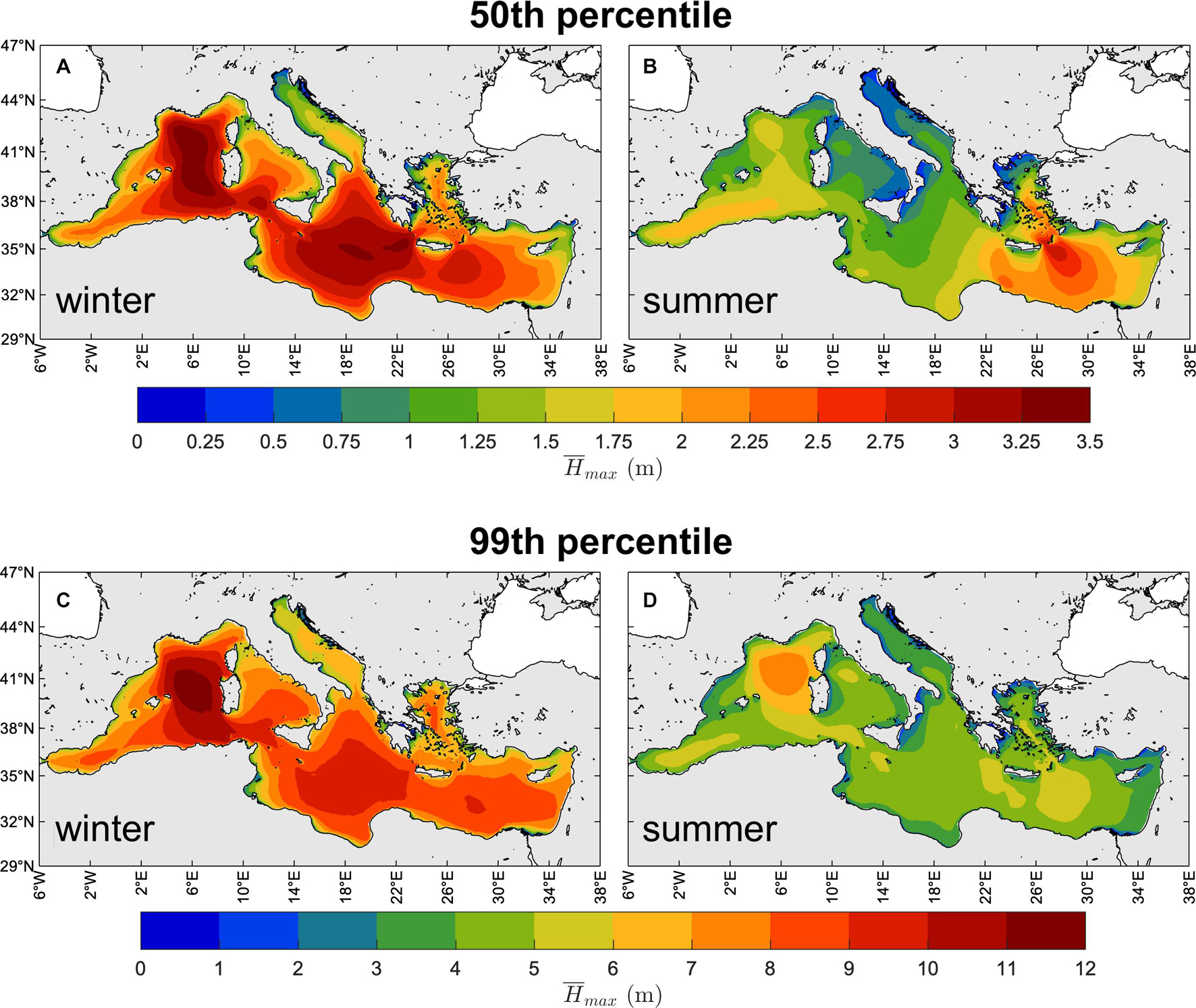
Figure 10. Climate of the maximum individual waves. Yearly-averaged seasonal 50th [panels (A,B)] and 99th [panels (C,D)] percentiles of ${\overline{H}}_{max}$ (1981–2019): winter [NDJFM, panels (A,C)], summer [JJA, right panels (B,D)].

The variability of the maximum individual wave climate (${\overline{C}}_{max}$ and ${\overline{H}}_{max}$) well matches the variability of the H_s climate, shown in section “Variability of the Mediterranean Sea Wind-Wave Climate.” The extreme-to-typical condition variations at seasonal scale for ${\overline{H}}_{max}$ and ${\overline{C}}_{max}$ are shown in Supplementary Figures 8, 9, respectively. Compared to the H_s variations in Figure 6, they only show minor differences, which do not substantially change the conclusions drawn about the seasonal and regional characteristics of the wave climate variability in the MS, which are also valid for the inter-annual variability.

What deserves more attention is the change in the maximum individual wave climate, expressed using the Sen’s slope of the linear trend over 1981–2019. Trends are shown in detail for ${\overline{H}}_{max}$ in Figure 11 (in Supplementary Figure 10 for ${\overline{C}}_{\text{max}}$) and summarized as spatial averages over the MS and sub-basins in Table 2 (in Supplementary Table 2 for ${\overline{C}}_{\text{max}}$). On average, maximum individual waves change more than H_s (Table 1) with slopes larger than H_s slopes: e.g., on average for the MS in winter 2.5 and 13.9 cm decade^–1 for ${\overline{H}}_{\text{max}}$, instead of 1.1 and 6.5 cm decade^–1 for corresponding H_s values. More than doubled slopes for ${\overline{H}}_{\text{max}}$ are also observed in Figure 11, with winter ${\overline{H}}_{\text{max}}$ increasing up to 10 cm decade^–1 in the Western sub-basin (50th percentile) and up to 25 cm decade^–1 in the Levantine sub-basin (99th percentile). In general, however, the spatial distribution of the trends for ${\overline{H}}_{\text{max}}$ (and ${\overline{C}}_{\text{max}}$ too) reflects the distribution of H_s trends. The meaning of these trends and how they can be interpreted compared to the H_s trends will be examined in the Discussion section.

FIGURE 11

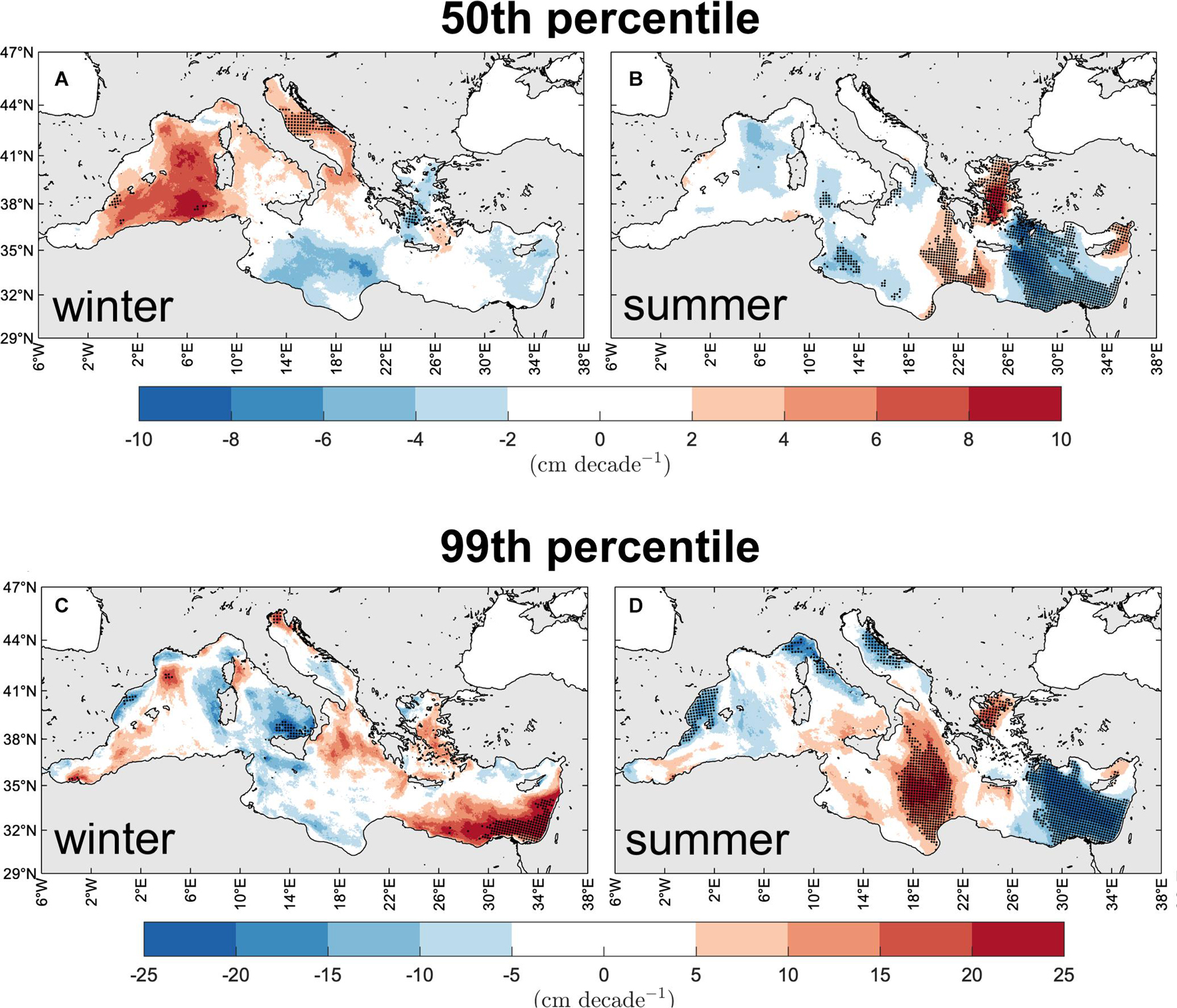
Figure 11. Change of the MS typical [50th percentile, panels (A,B)] and extreme [99th percentile, panels (C,D)] maximum individual wave climate. Trend of the winter [panels (A,C)] and summer [panels (B,D)] ${\overline{H}}_{max}$ during 1981–2019. Areas with statistically significant trends at the 90% confidence intervals are denoted by black dots (decimated for graphical purposes).

TABLE 2

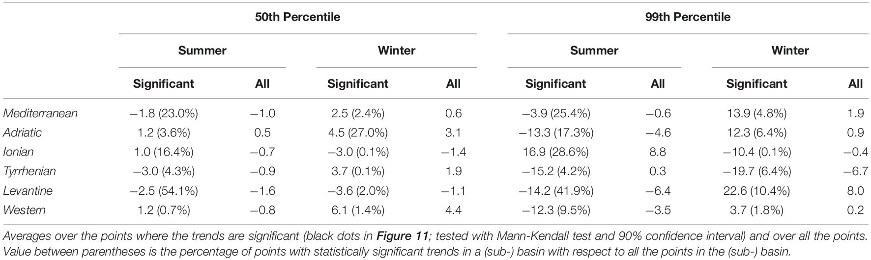
Table 2. Spatial averages over the MS and sub-basins of the 50th and 99th percentile ${\overline{H}}_{max}$ trends shown in Figure 11 (cm decade^–1), during 1981–2019 summer and winter seasons.

Wave Steepness and Narrow Bandedness

We have shown that, while the maximum individual wave climate displays characteristic typical and extreme values, spatial patterns and variability of the maximum individual wave climate closely mirror those of the significant wave height. The reason is that maximum crest and wave heights are monotonic functions of significant wave height H_s [see Equations (1) and (2)]. Therefore, we expect that regions where H_s is large are also the regions where ${\overline{C}}_{max}$ and ${\overline{H}}_{max}$ are the highest. This is confirmed by the comparison of Figure 10 and Supplementary Figure 7. At the same time, though with a smaller effect with respect to H_s, ${\overline{C}}_{max}$ and ${\overline{H}}_{max}$ are also monotonic functions of the wave steepness μ and the narrow bandedness ψ^∗, respectively [see Equations (1) and (2)]. Therefore, maximum individual wave heights in Figure 10 and Supplementary Figure 7 are the result of the combined effect of H_s (both ${\overline{C}}_{max}$ and ${\overline{H}}_{max}$), μ (${\overline{C}}_{max}$) and ψ^∗ (${\overline{H}}_{max}$).

In Figures 12A,B we show the yearly-averaged winter and summer 50th percentile of μ. As younger waves are generally steeper, largest steepness (up to 0.07) can be found close to the shores where prevailing Mediterranean onshore winds blow from: e.g., in the Gulf of Lyon (Mistral), in the Aegean Sea (Etesian), along the eastern Adriatic coast (Bora), but also on the leeward side of straits (i.e., Sirocco to the north of Otranto Strait in the Adriatic Sea, Vendaval to the east of Gibraltar Strait, Mistral to the east of Bonifacio Strait in the Tyrrhenian Sea, Etesian to the west of the Bosporus Strait). Steepness decreases moving off-shore along the wind direction as waves develop. Although the steepest waves occur in winter, the summer Etesian wind waves are as steep as in winter. The 99th percentile of μ (Figures 12C,D), again larger in correspondence of younger waves, is up to 0.075 over the whole MS except in the Adriatic Sea (up to 0.08) and in very narrow coastal regions where can be up to 0.09. Wind-sea dominated seas typically have steepness values larger than 0.03–0.04, while swell dominated seas may have halved values compared to wind-seas (Barbariol et al., 2019). The steepness values we find in the MS (generally larger than 0.03) denotes the predominance of wind-seas in the MS climate, especially in winter. During summer smaller values (0.02; 50th percentile) can be found in the Gulf of Genoa and in the southern Tyrrhenian Sea, where mature waves driven by south-westerly winds can develop after frequency- and direction-dispersion along the large distances from the Alboran Sea to these areas (among the longest in the MS).

FIGURE 12

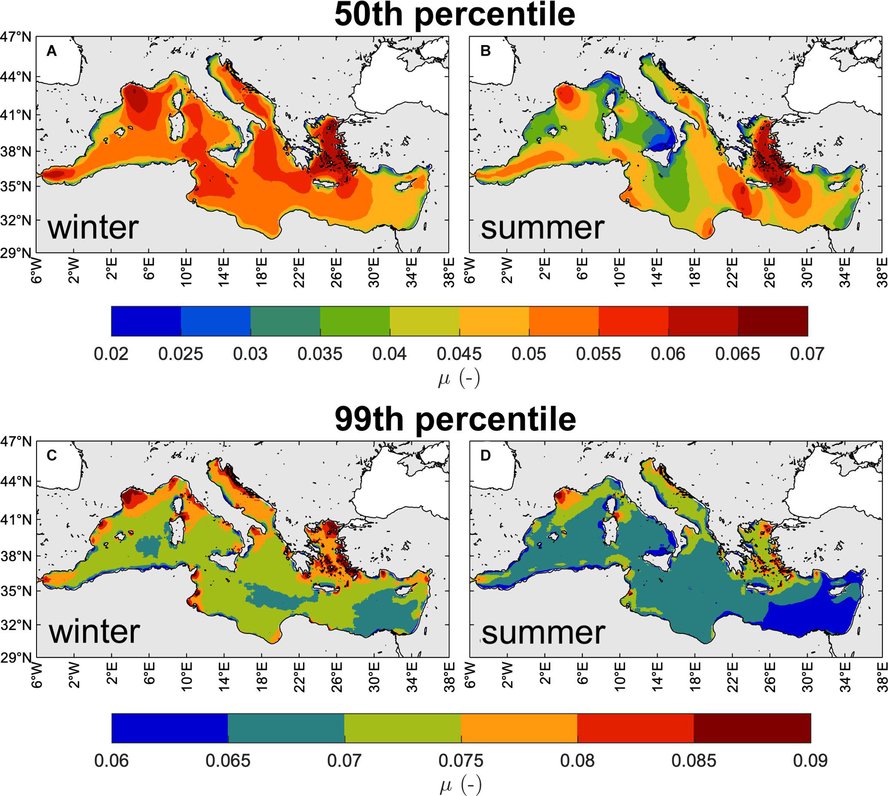
Figure 12. Yearly-averaged seasonal 50th [panels (A,B)] and 99th [panels (C,D)] percentiles of μ (1981–2019): winter [NDJFM, panels (A,C)], summer [JJA, panels (B,D)].

The yearly-averaged 50th percentile of ψ^∗, shown in Figures 13A,B, generally ranges between 0.625 and 0.675 in winter, while can be up to 0.75 in summer. These are values representative of a unimodal wind-sea (0.65 ≤ ψ^∗ ≤ 0.75; see Boccotti, 2000), denoting the prevailing nature of typical MS sea states. Smaller values can be found in the wide western and southern basins where a local wind-sea may combine with more mature seas coming from different directions. It is worth mentioning that a proper long-term statistical analysis of the sea state characteristics should account for different wave systems separately. That is, wind-sea and swell (if any) should be separated (e.g., using spectral partitioning techniques accounting also for wave direction) and treated independently as they have a different origin and belong statistically to different populations. However, the range of superimposed wind-sea and swell (ψ^∗ ≤ 0.6; Boccotti, 2000) is rather rare in the MS, even if crossing sea states with waves with different wave direction may occur. The 99th percentile values of ψ^∗ (Figures 13C,D), generally larger than 0.7 and up to 1, denotes the presence of narrow banded sea states, able to produce the largest crest-to-trough excursions according to the Quasi-Determinism theory (Boccotti, 2000; Benetazzo et al., 2017, 2021b), especially in the Adriatic, Tyrrhenian and Aegean seas.

FIGURE 13

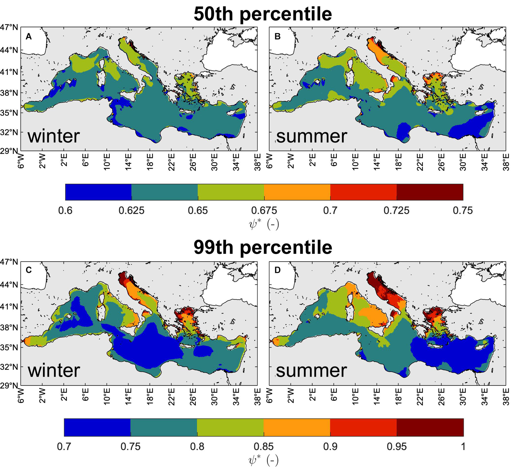
Figure 13. Yearly-averaged seasonal 50th [panels (A,B)] and 99th [panels (C,D)] percentiles of ψ^∗ (1981–2019): winter [NDJFM, panels (A,C)], summer [JJA, panels (B,D)].

Discussion

In this section, we first highlight and discuss the limits and strengths of the dataset and of the related climate analysis. Then, we comment on the results we have obtained, by also comparing them to those obtained in previous studies for the same area.

The climatology of MS waves presented in the previous section relies upon the climatology of the ERA5 reanalysis wind. Even if ERA5 horizontal resolution may be poor for representing the dynamical structure of the wind fields in some regional seas, as the narrow semi-enclosed Adriatic or Aegean seas, it currently represents the state-of-the-art of long-term atmospheric reanalysis and hence the best forcing option for the present work. In this context, using a dynamical downscaling of ERA5 winds, Vannucchi et al. (2021) showed an improvement of wind and wave hindcast performance against wind stations and buoys in the MS compared to the original ERA5 data mostly at coastal stations. We have decided to use ERA5 wind and not ERA5 waves, as the latter may be not suitable for long-term climate analyses, at least for studies extending before and after 1992, i.e., the beginning of satellite altimeter data assimilation in the wave models. The introduction of spurious trends is a well-known issue pointed out by Aarnes et al. (2015) for ERA-Interim reanalysis waves (Dee et al., 2011) that may apply also to ERA5. To cope with the resolution issue of ERA5 in the MS and with the potential 1992 singularity in wave products, we have therefore (i) relied on the ERA5 wind forcing (on which we expect a smaller or at least indirect data assimilation effect) and on an ad hoc high-resolution (about 5 km) wave hindcast and (ii) verified the wave hindcast results against satellite altimetry. While this has not increased the wind forcing resolution, it has allowed us to produce one of the longest consistent Mediterranean wave hindcasts up to now, providing a detailed representation of the wave climatology in a morphologically complex enclosed sea and assessing its uncertainty compared to observations in the region. Concerning the hindcast performance, the MS wave climate, its (intra- and inter-annual) variability and the trends have shown to be well reproduced by the ERA5 wind forced hindcast. However, the negative modeled-observed H_s relative bias shown in Section “Assessment of the Mediterranean Ses Wind-Wave Hindcast” should be regarded when using the estimates of the 50th and 99th percentile of the MS wave heights.

Results of the wave hindcast and following wave climate analysis have shown marked regional characteristics of the wave climate, related to the peculiarities of the regional winds blowing over the Mediterranean sub-basins. Results for the typical and extreme wind-wave climate are in agreement with other studies both for spatial distribution and intensity, albeit with some differences [see e.g., Morales-Márquez et al. (2020) for extreme winter H_s and Lionello and Sanna (2005) for mean seasonal H_s, both presenting slightly smaller maxima]. In particular, results have highlighted the MS regions where the largest waves occur, which are in the Western, Ionian and Levantine sub-basins, depending on the season. Indeed, compared to previous studies, in this paper we have provided results at a seasonal scale. We have shown that the variety of the MS wave climate characteristics may be well represented by winter and summer seasons, in terms of intensity and patterns of wave heights, with spring and autumn in-between. This is in agreement with the results of Lionello and Sanna (2005), who argued that the MS climate, including wave climate, is characterized by two main seasons, i.e., winter and summer, with spring and autumn only being transitional seasons.

The definition of seasons we have adopted in this study is based on the wind-wave climate and on the altimeter H_s observations in particular, rather than on monthly air temperatures, as in the meteorological definition of seasons. This choice is supported by other studies on the MS region climate. Indeed, Trigo et al. (1999) suggested that the traditional four meteorological seasons do not fit well the cyclone occurrence patterns in the MS region. In this context, attempts to objectively define season start/end and duration in the MS region, based on different indices than the largely spatially variable temperature, led to definitions of seasons that generally correspond to the traditional ones, but with longer winters and shorter springs and autumns (Alpert et al., 2004; Kotsias et al., 2021) in agreement with our definition. Also Lionello and Sanna (2005), based on principal component analysis of the modeled H_s, defined four seasons, again with longer winters (and summers) and shorter springs and autumns.

Following the conclusions of previous studies that found that the climate (including wave climate) variability of part of the MS (in particular the northern part with a mid-latitude climate regime) can be partially related to midlatitude climate indices (e.g., Lionello and Sanna, 2005; Morales-Márquez et al., 2020) we have searched for teleconnections between wave climate variability and the principal modes of atmospheric variability. We have found that MS typical (50th percentile) wave climate variability is generally positively correlated to the SCAND index (i.e., positive H_s anomalies generally corresponding to positive SCAND phases, and viceversa). This is in accordance with the SCAND positive phases being generally associated with enhanced cyclogenesis in the MS region (Xoplaki, 2002). Extreme wave variability (99th percentile) is also positively correlated to the SCAND index in summer, while it can be negatively correlated to the EA index in winter. The negative phases of EA were also related to extreme waves in the MS by Izaguirre et al. (2010) using satellite data. Over the sub-basins there can be differences, for example the Adriatic Sea, whose wave climate variability is always positively correlated to the SCAND index during winter and to EAWR during summer. In general, our results are in agreement with the results from another study (Morales-Márquez et al., 2020) and suggest that the MS wave climate variability is mildly-to-slightly related to the variability of large-scale atmospheric structures, which have a more clear influence on the wave climate in other seas (e.g., the North-Atlantic Ocean; Morales-Márquez et al., 2020). We thus share the conclusions of Lionello and Galati (2008) that even if some patterns seem to exert a larger influence with respect to others, this is not sufficient to explain the dominant variability of the wave climate in the MS and its sub-basins, which is the result of a combined effect of large-scale atmosphere dynamics and orography (forcing regional winds).

The observed trend of decreasing H_s during summer and increasing H_s during winter (both for typical and extreme wave climate; Table 1) seems to disagree with some other past climate change studies in the region, although based on different wind forcing datasets, wave models, trend estimate, and season definition. Indeed, Lionello and Sanna (2005) found a statistically significant decreasing trend of the mean H_s in the MS during winter months (December to March, −2.4 cm decade^–1), while we have found a statistically significant increasing trend of the median H_s in the MS during November to March (Table 1, 1.1 cm decade^–1). Also, the spatial distribution and intensity of the 99th percentile winter (December to February) H_s trend obtained by Morales-Márquez et al. (2020) only partially resembles that shown in Figure 9C. There is instead remarkable agreement, at least in some specific regions, with the trend estimates for the annual maximum H_s by De Leo et al. (2020). Comparing those estimates with ours for the winter 99th percentile H_s (the closest to the annual maxima), we see many areas of corresponding increase/decrease: for instance, positive trends in the Gulf of Lyon and other parts of the Western basin, in the northern Adriatic and Tyrrhenian seas and in the easternmost part of the Levantine basin; negative trends in the southern Tyrrhenian Sea, Sardinian Sea and central Adriatic Sea. However, the change in the wind-wave climate we have found (Figure 9 and Table 1) reflects the change in the ERA5 wind forcing intensity and spatial distribution while for instance Lionello and Sanna (2005) study is based on the ERA-40 reanalysis (Uppala et al., 2005) and Morales-Márquez et al. (2020) and De Leo et al. (2020) on the CFSR reanalysis (Chawla et al., 2013). Hence, the reasons for different trends on the intensity of storms should be searched for in the wind forcings that have generated the wave model results. Changes in ERA5 wind characteristics might be due, for instance, to changes in storm trajectories, as suggested by numerous climatological studies, which investigated not only the intensity and frequency of Mediterranean cyclones but also the variability of their trajectories in the last decades and in the future climate projections (Lionello et al., 2002; Lionello and Giorgi, 2007; Cavicchia et al., 2014; Messmer et al., 2020). We have verified monthly H_s percentile trends from the ERA5 wind forced wave hindcast at the MS basin scale against trends from satellite altimeters and found a general agreement in the increasing/decreasing trends as well as in the magnitude of the trends. For ${\overline{H}}_{max}$ (and ${\overline{C}}_{max})$, we have found trends that are larger than the H_s trends: for instance, for the winter 50th percentile on the whole MS, on average 2.44 times for ${\overline{H}}_{max}$. This can be explained with ${\overline{H}}_{max}$ being on average 2.36H_s. Hence, the linear trend of ${\overline{H}}_{max}$, i.e., $\mathrm{△}{\overline{H}}_{max}/\mathrm{△}T$, should be on average $\mathrm{△}{\overline{H}}_{max}/\mathrm{△}T\approx 2.36\mathrm{△}{H}_s/\mathrm{△}T$, the difference between 2.44 and 2.36 being possibly explained with a change in the other wave parameters that ${\overline{H}}_{max}$ depends upon.

Conclusion

In this paper, we have taken advantage of the ERA5 atmospheric wind reanalysis and spectral wave modeling to characterize the wind-wave climate of the MS, its spatio-temporal variability and change. The wind-wave dataset we have produced has allowed us to obtain one of the longest wave climate assessments in the MS to date. Also, for the first time we have bestowed an assessment of the maximum individual wave climate in the MS. Our main results are here summarized:

• We have verified the ERA5 wind-based wind-wave hindcast against satellite observations of significant wave height with respect to its performance in reproducing the typical (50th percentile) and extreme (99th percentile) H_s, and the variability and trend of the MS wind-wave climate. Despite a general tendency to underestimate H_s (in particular in narrow basins as the Adriatic Sea and for the extremes) the dataset has been shown to properly reproduce the temporal variability and the trends of H_s.

• We have presented the typical and extreme MS wind-wave climate patterns and characteristics at seasonal scale and, to this end, we have proposed and used a definition of seasons based on the satellite observation of significant wave height over the MS, which presents a stormy season (winter) lasting 5 months, a calm season (summer) lasting 3 months and two transitional seasons (spring and autumn) lasting 2 months each. This definition is in agreement with other objective season definitions in the MS.

• The largest typical waves (both as H_s and maximum individual waves) occur in the western and southern MS during winter, and in the eastern MS during summer, whereas the largest extreme waves occur in the western MS in all seasons, with maximum values during winter.

• The intra-seasonal variability of MS wind waves (expressed as the ratio of the 99th to the 50th percentile H_s) has been shown to be largest during summer and in the Adriatic, Tyrrhenian and Sardinian Seas, indicating these are season and the MS sub-basins that are more prone to the development of large extremes waves compared to the typical ones. On the other hand, the inter-annual variability has proven to be largest where the largest winter and summer waves occur. However, when the inter-annual variability has been expressed with respect to the local climate (i.e., in terms of relative anomaly) it has emerged that the Adriatic and Tyrrhenian Seas are characterized by the largest variability of typical and extreme H_s, with the Ionian and Levantine sub-basins also showing large variability of extreme H_s. During the analyzed period (1981–2019) these regions of the MS have experienced variations up to 100% of both the local 50th or 99th percentile H_s.

• We have motivated the largest positive and negative relative anomalies of H_s in the MS basin (and sub-basins) thanks to the geopotential height at 500 hPa, mean sea level pressure and wind intensity anomalies and we have related the temporal variability of the relative anomalies in the MS to the principal modes of atmospheric variability. The seasonal Scandinavian index seems the most correlated to the seasonal wind-wave variability in the MS, especially during winter and for the typical H_s, with positive Scandinavian index phases associated to the largest typical winter H_s (extreme winter H_s are best correlated to the Eastern Atlantic index). However, correlations found are not remarkable (0.54 at most for the MS, 0.65 for sub-basins) and this suggests, in agreement with previous studies in the MS, that the wind-wave variability in the MS can only be partially motivated by teleconnections, most likely due to the effects of local orography that, interacting with synoptic scale atmospheric structures, generates cyclones and consequent winds with regional characteristics that partially lose the link with their large-scale source.

• The long-term trends found in the ERA5-wind based hindcast of the MS waves are negative for the summer season and positive for the winter season, both for typical and extreme sea states (and maximum individual waves). These trends are statistically significant though generally modest in magnitude (however, locally up to 12 cm decade^–1 for extreme winter H_s and 25 cm decade^–1 for extreme winter ${\overline{H}}_{max}$) and are larger for extreme sea states compared to typical sea states. This suggests the MS wind-wave climate has changed during 1981–2019, with decreasing H_s (and maximum individual waves) during summer and increasing during winter.

• The climate characteristics (patterns, spatio-temporal variability and change) of maximum individual waves closely mirror those of H_s, although there are some differences that are motivated by the dependence of ${\overline{H}}_{max}$ (and ${\overline{C}}_{max}$) by other sea state characteristics, i.e., the narrow bandedness parameter and the wave steepness. We have presented their typical and extreme seasonal patterns and intensities, showing that MS sea states are generally dominated by wind waves.

Concluding, this study have proven that the ERA5 wind can be successfully used to hindcast the wind waves in the MS, a crucial task to assess the past and present climate in a regional basin providing environmental and economical services to the whole MS region and where the impacts of climate change are expected to be significant in the near future. As a recommendation for future reanalysis-wind based assessments in a semi-enclosed basin with similar characteristics (i.e., narrow sub-basins and surrounding orography), in order to reduce the spatial resolution effects in the narrowest basins (as the Adriatic Sea) and close to the coasts, a dynamical downscaling of ERA5 winds would be advisable. This represents one of the further improvements on the hindcast production side. As regards the wave climate analysis, although swell seas are rather rare in the MS, a partitioning analysis of the directional wave spectra determining the different wave systems that may mix in a sea state would allow treating them separately (if necessary) and also characterizing the crossing seas that often pose serious problems to ships in navigation. Finally, further investigations, for instance looking for a change in the direction of cyclonic paths and their intensity, would help disentangling the dominant mechanisms that drive the changing seasonal wave climate we found.

Data Availability Statement

The raw data supporting the conclusions of this article will be made available by the authors, without undue reservation.

Author Contributions

FB, SD, and AB contributed to the conception and design of the study and produced the dataset. FB and SD performed the dataset assessment. FB and AR performed the analyses. SD, FF, RF, MS, and AB contributed to the analyses. FB wrote the manuscript. All authors contributed to manuscript revision, read, and approved the submitted version.

Funding

This study was partially supported by the Copernicus Marine Environment Monitoring Service (CMEMS) LATEMAR project. CMEMS is implemented by Mercator Ocean in the framework of a delegation agreement with the European Union. This work has also been conducted as part of the bilateral project EOLO-1 (“Extreme oceanic waves during tropical, tropical-like, and bomb cyclones”) between CNR-ISMAR and the University of Tokyo (Japan). Antonio Ricchi funding has been provided by PON Ricerca e Innovazione 2014–2020 “AIM”—Attraction and international mobility program. EU Social Fund and Regional Development Fund; Ministero dell’Istruzione e della Ricerca, grant number AIM1858058.

Conflict of Interest

The authors declare that the research was conducted in the absence of any commercial or financial relationships that could be construed as a potential conflict of interest.

Publisher’s Note

All claims expressed in this article are solely those of the authors and do not necessarily represent those of their affiliated organizations, or those of the publisher, the editors and the reviewers. Any product that may be evaluated in this article, or claim that may be made by its manufacturer, is not guaranteed or endorsed by the publisher.

Acknowledgments

Hersbach et al. (2018) was downloaded from the Copernicus Climate Change Service (C3S) Climate Data Store. The results contain modified Copernicus Climate Change Service information, 2020. Neither the European Commission nor ECMWF is responsible for any use that may be made of the Copernicus information or data it contains. We would like to thank Luigi Cavaleri for fruitful discussions on the topic.

Supplementary Material

The Supplementary Material for this article can be found online at: https://www.frontiersin.org/articles/10.3389/fmars.2021.760614/full#supplementary-material

Footnotes

1. ^ https://polar.ncep.noaa.gov/waves/
2. ^ https://catalogue-imos.aodn.org.au
3. ^ https://www.cpc.ncep.noaa.gov/data/teledoc/telecontents.shtml

References

Aarnes, O. J., Saleh, A., Jean, R. B., and Øyvind, B. (2015). Marine wind and wave height trends at different ERA-interim forecast ranges. J. Clim. 28, 819–837. doi: 10.1175/JCLI-D-14-00470.1

CrossRef Full Text | Google Scholar

Alpert, P., Osetinsky, I., Ziv, B., and Shafir, H. (2004). A new seasons definition based on classified daily synoptic systems: an example for the Eastern Mediterranean. Int. J. Climatol. 24, 1013–1021. doi: 10.1002/joc.1037

CrossRef Full Text | Google Scholar

Ardhuin, F., Rogers, E., Babanin, A. V., Filipot, J.-F., Magne, R., Roland, A., et al. (2010). Semiempirical dissipation source functions for ocean waves. Part I: definition, calibration, and validation. J. Phys. Oceanogr. 40, 1917–1941. doi: 10.1175/2010JPO4324.1

CrossRef Full Text | Google Scholar

Arena, F., Laface, V., Malara, G., Romolo, A., Viviano, A., Fiamma, V., et al. (2015). Wave climate analysis for the design of wave energy harvesters in the Mediterranean Sea. Renew. Energy 77, 125–141. doi: 10.1016/j.renene.2014.12.002

CrossRef Full Text | Google Scholar

Barbariol, F., Alves, J. H. G. M., Benetazzo, A., Bergamasco, F., Bertotti, L., Carniel, S., et al. (2017). Numerical modeling of space-time wave extremes using WAVEWATCH III. Ocean Dyn. 67, 535–549. doi: 10.1007/s10236-016-1025-0

CrossRef Full Text | Google Scholar

Barbariol, F., Benetazzo, A., Carniel, S., and Sclavo, M. (2013). Improving the assessment of wave energy resources by means of coupled wave-ocean numerical modeling. Renew. Energy 60, 462–471. doi: 10.1016/j.renene.2013.05.043

CrossRef Full Text | Google Scholar

Barbariol, F., Bidlot, J.-R., Cavaleri, L., Sclavo, M., Thomson, J., and Benetazzo, A. (2019). Maximum wave heights from global model reanalysis. Prog. Oceanogr. 175, 139–160. doi: 10.1016/j.pocean.2019.03.009

CrossRef Full Text | Google Scholar

Battjes, J., and Janssen, J. P. F. M. (1978). “Energy loss and set-up due to breaking of random waves,” in Proceedings of the 16th International Conference on Coastal Engineering, Vol. 1, (New York, NY: American Society of Civil Engineers), 569–587. doi: 10.9753/icce.v16.32

CrossRef Full Text | Google Scholar

Benetazzo, A., Barbariol, F., Pezzutto, P., Staneva, J., Behrens, A., Davison, S., et al. (2021b). Towards a unified framework for extreme sea waves from spectral models: rationale and applications. Ocean Eng. 219:108263.

Google Scholar

Benetazzo, A., Barbariol, F., Bergamasco, F., Bertotti, L., Yoo, J., Shim, J.-S., et al. (2021a). On the extreme value statistics of spatio-temporal maximum sea waves under cyclone winds. Prog. Oceanogr. 197:102642. doi: 10.1016/j.pocean.2021.102642

CrossRef Full Text | Google Scholar

Benetazzo, A., Barbariol, F., Bergamasco, F., Carniel, S., and Sclavo, M. (2017). Space-time extreme wind waves: analysis and prediction of shape and height. Ocean Model. 113, 201–216. doi: 10.1016/j.ocemod.2017.03.010

CrossRef Full Text | Google Scholar

Benetazzo, A., Fedele, F., Carniel, S., Ricchi, A., Bucchignani, E., and Sclavo, M. (2012). Wave climate of the adriatic sea: a future scenario simulation. Nat. Hazards Earth Syst. Sci. 12, 2065–2076. doi: 10.5194/nhess-12-2065-2012

CrossRef Full Text | Google Scholar

Bertotti, L., and Cavaleri, L. (2008). The predictability of the ‘Voyager’ accident. Nat. Hazards Earth Syst. Sci. 8, 533–537. doi: 10.5194/nhess-8-533-2008

CrossRef Full Text | Google Scholar

Besio, G., Mentaschi, L., and Mazzino, A. (2016). Wave energy resource assessment in the Mediterranean Sea on the basis of a 35-year Hindcast. Energy 94, 50–63. doi: 10.1016/j.energy.2015.10.044

CrossRef Full Text | Google Scholar

Boccotti, P. (2000). Wave Mechanics for Ocean Engineering. New York, NY: Elsevier Science B.V., 496.

Google Scholar

Cavaleri, L., Bajo, M., Barbariol, F., Bastianini, M., Benetazzo, A., Bertotti, L., et al. (2019). The October 29, 2018 storm in Northern Italy – an exceptional event and its modeling. Prog. Oceanogr. 178:102178. doi: 10.1016/j.pocean.2019.102178

CrossRef Full Text | Google Scholar

Cavaleri, L., Fox-Kemper, B., and Hemer, M. (2012b). Wind waves in the coupled climate system. Bull. Am. Meteorol. Soc. 93, 1651–1661. doi: 10.1175/BAMS-D-11-00170.1

CrossRef Full Text | Google Scholar

Cavaleri, L., Bertotti, L., Torrisi, L., Bitner-Gregersen, E., Serio, M., and Onorato, M. (2012a). Rogue waves in crossing seas: the Louis Majesty accident. J. Geophys. Res. Oceans 117:C00J10. doi: 10.1029/2012JC007923

CrossRef Full Text | Google Scholar

Cavicchia, L., Von Storch, H., and Gualdi, S. (2014). Mediterranean tropical-like cyclones in present and future climate. J. Clim. 27, 7493–7501. doi: 10.1175/JCLI-D-14-00339.1

CrossRef Full Text | Google Scholar

Chawla, A., Spindler, D. M., and Tolman, H. L. (2013). Validation of a thirty year wave hindcast using the climate forecast system reanalysis winds. Ocean Model. 70, 189–206. doi: 10.1016/j.ocemod.2012.07.005

CrossRef Full Text | Google Scholar

De Leo, F., Besio, G., and Mentaschi, L. (2021). Trends and variability of ocean waves under RCP8.5 emission scenario in the Mediterranean Sea. Ocean Dyn. 71, 97–117. doi: 10.1007/s10236-020-01419-8

CrossRef Full Text | Google Scholar

De Leo, F., De Leo, A., Besio, G., and Briganti, R. (2020). Detection and quantification of trends in time series of significant wave heights: an application in the Mediterranean Sea. Ocean Eng. 202:107155. doi: 10.1016/j.oceaneng.2020.107155

CrossRef Full Text | Google Scholar

Dee, D. P., Uppala, S. M., Simmons, A. J., Berrisford, P., Poli, P., Kobayashi, S., et al. (2011). The ERA-interim reanalysis: configuration and performance of the data assimilation system. Q. J. R. Meteorol. Soc. 137, 553–597. doi: 10.1002/qj.828

CrossRef Full Text | Google Scholar

DNV GL–Det Norske Veritas Germanischer Lloyd (2017). DNVGL-RP-C205: Environmental Conditions and Environmental Loads. DNV GL Recommended Practice. Oslo: DNV GL, 1–259.

Google Scholar

Dysthe, K., Krogstad, H. E., and Müller, P. (2008). Oceanic rogue waves. Annu. Rev. Fluid Mech. 40, 287–310.

Google Scholar

Fedele, F. (2012). Space–time extremes in short-crested storm seas. J. Phys. Oceanogr. 42, 1601–1615.

Google Scholar

Giorgi, F. (2006). Climate change hot-spots. Geophys. Res. Lett. 33:L08707. doi: 10.1029/2006GL025734

CrossRef Full Text | Google Scholar

Hasselmann, K., Barnett, T. P., Bouws, E., Carlson, H., Cartwright, D. E., Enke, K., et al. (1973). Measurements of Wind-Wave Growth and Swell Decay During the Joint North Sea Wave Project (JONSWAP). Hamburg: Deutsches Hydrographisches Institut Hamburg.

Google Scholar

Hersbach, H., Bell, B., Berrisford, P., Biavati, G., Horányi, A., Muñoz Sabater, J., et al. (2018). ERA5 Monthly Averaged Data on Single Levels from 1979 to Present. Copernicus Climate Change Service (C3S) Climate Data Store (CDS).

Google Scholar

Hersbach, H., Bell, B., Berrisford, P., Hirahara, S., Horányi, A., Muñoz-Sabater, J., et al. (2020). The ERA5 global reanalysis. Q. J. R. Meteorol. Soc. 146, 1999–2049. doi: 10.1002/qj.3803

CrossRef Full Text | Google Scholar

Izaguirre, C., Mendez, F. J., Menendez, M., Luceño, A., and Losada, I. J. (2010). Extreme wave climate variability in Southern Europe using satellite data. J. Geophys. Res. 115:C04009. doi: 10.1029/2009jc005802

CrossRef Full Text | Google Scholar

Kendall, M. G. (1948). Rank Correlation Methods. London: C. Griffin.

Google Scholar

Kotsias, G., Lolis, C. J., Hatzianastassiou, N., Lionello, P., and Bartzokas, A. (2021). An objective definition of seasons for the Mediterranean region. Int. J. Climatol. 41, E1889–E1905. doi: 10.1002/joc.6819

CrossRef Full Text | Google Scholar

Liberti, L., Carillo, A., and Sannino, G. (2013). Wave energy resource assessment in the {M}editerranean, the {I}talian perspective. Renew. Energy 50, 938–949. doi: 10.1016/j.renene.2012.08.023

CrossRef Full Text | Google Scholar

Lionello, P. (2012). The Climate of the Mediterranean Region. Amsterdam: Elsevier. doi: 10.1016/C2011-0-06210-5

CrossRef Full Text | Google Scholar

Lionello, P., Dalan, F., and Elvini, E. (2002). Cyclones in the Mediterranean region: the present and the doubled CO2 climate scenarios. Clim. Res. 22, 147–159. doi: 10.3354/cr022147

CrossRef Full Text | Google Scholar

Lionello, P., and Galati, M. B. (2008). Links of the significant wave height distribution in the Mediterranean sea with the Northern hemisphere teleconnection patterns. Adv. Geosci. 17, 13–18. doi: 10.5194/adgeo-17-13-2008

CrossRef Full Text | Google Scholar

Lionello, P., and Giorgi, F. (2007). Winter precipitation and cyclones in the Mediterranean region: future climate scenarios in a regional simulation. Adv. Geosci. 12, 153–158. doi: 10.5194/adgeo-12-153-2007

CrossRef Full Text | Google Scholar

Lionello, P., and Sanna, A. (2005). Mediterranean wave climate variability and its links with NAO and Indian monsoon. Clim. Dyn. 25, 611–623. doi: 10.1007/s00382-005-0025-4

CrossRef Full Text | Google Scholar

Mann, H. B. (1945). Nonparametric tests against trend. Econometrica 13, 245–259. doi: 10.2307/1907187

CrossRef Full Text | Google Scholar

Mentaschi, L., Besio, G., Cassola, F., and Mazzino, A. (2015). Performance evaluation of WAVEWATCH III in the Mediterranean sea. Ocean Model. 90, 82–94. doi: 10.1016/j.ocemod.2015.04.003

CrossRef Full Text | Google Scholar

Messmer, M., Raible, C. C., and ómez-Navarro, J. J. G. (2020). Impact of climate change on the climatology of Vb cyclones. Tellus Ser. A Dyn. Meteorol. Oceanogr. 72, 1–18. doi: 10.1080/16000870.2020.1724021

CrossRef Full Text | Google Scholar

Morales-Márquez, V., Orfila, A., Simarro, G., and Marcos, M. (2020). Extreme waves and climatic patterns of variability in the Eastern North Atlantic and Mediterranean Basins. Ocean Sci. 16, 1385–1398. doi: 10.5194/os-16-1385-2020

CrossRef Full Text | Google Scholar

Piante, C., and Ody, D. (2015). Blue Growth in the Mediterranean Sea: The Challenge of Good Environmental Status. MedTrends Project. WWF, 192. Available online at: http://www.developpement-durable.gouv.fr/ (accessed October 20, 2021).

Google Scholar

Portilla-Yandún, J., Barbariol, F., Benetazzo, A., and Cavaleri, L. (2019). On the statistical analysis of ocean wave directional spectra. Ocean Eng. 189:106361. doi: 10.1016/j.oceaneng.2019.106361

CrossRef Full Text | Google Scholar

Queffeulou, P., and Bentamy, A. (2007). Analysis of wave height variability using altimeter measurements: application to the Mediterranean Sea. J. Atmos. Ocean. Technol. 24, 2078–2092. doi: 10.1175/2007JTECH0507.1

CrossRef Full Text | Google Scholar

Ribal, A., and Young, I. R. (2019). 33 years of globally calibrated wave height and wind speed data based on altimeter observations. Sci. Data 6:77. doi: 10.1038/s41597-019-0083-9

PubMed Abstract | CrossRef Full Text | Google Scholar

Sartini, L., Besio, G., and Cassola, F. (2017). Spatio-temporal modelling of extreme wave heights in the Mediterranean Sea. Ocean Model. 117, 52–69. doi: 10.1016/j.ocemod.2017.07.001

CrossRef Full Text | Google Scholar

Sartini, L., Cassola, F., and Besio, G. (2015a). Extreme waves seasonality analysis: an application in the Mediterranean Sea. J. Geophys. Res. Oceans 120, 6266–6288. doi: 10.1002/2015JC011061

CrossRef Full Text | Google Scholar

Sartini, L., Mentaschi, L., and Besio, G. (2015b). Comparing different extreme wave analysis models for wave climate assessment along the Italian Coast. Coast. Eng. 100, 37–47. doi: 10.1016/j.coastaleng.2015.03.006

CrossRef Full Text | Google Scholar

Sen, P. K. (1968). Estimates of the regression coefficient based on Kendall’s Tau. J. Am. Stat. Assoc. 63, 1379–1389. doi: 10.1080/01621459.1968.10480934

CrossRef Full Text | Google Scholar

Tayfun, M. A. (1980). Narrow-band nonlinear sea waves. J. Geophys. Res. 85, 1548–1552.

Google Scholar

The WAVEWATCH III Development Group [WW3DG] (2016). User Manual and System Documentation of WAVEWATCH III Version 5.16. Technical Note, MMAB Contribution.

Google Scholar

The WAVEWATCH III Development Group [WW3DG] (2019). User Manual and System Documentation of WAVEWATCH III-Version 6.07. College Park, MD: WW3DG.

Google Scholar

Theil, H. (1950). A rank-invariant method of linear and polynomial regression analysis, part I. Proc. R. Neth. Acad. Sci. 53, 386–392.

Google Scholar

Tolman, H. L. (1991). A third-generation model for wind waves on slowly varying, unsteady, and inhomogeneous depths and currents. J. Phys. Oceanogr. 21, 782–797.

Google Scholar

Tolman, H. L. (2003). Treatment of unresolved islands and ice in wind wave models. Ocean Model. 5, 219–231. doi: 10.1016/S1463-5003(02)00040-9

CrossRef Full Text | Google Scholar

Trigo, I. F., Davies, T. D., and Bigg, G. R. (1999). Objective climatology of cyclones in the Mediterranean region. J. Clim. 12, 1685–1696. doi: 10.1175/1520-0442(1999)012<1685:OCOCIT>2.0.CO;2

CrossRef Full Text | Google Scholar

United Nations Environment Programme/Mediterranean Action Plan and Plan Bleu (2020). State of the Environment and Development in the Mediterranean. Nairobi: Marseille Imprimerie.

Google Scholar

Uppala, S. M., Kållberg, P. W., Simmons, A. J., Andrae, U., da Costa Bechtold, V., Fiorino, M., et al. (2005). The ERA-40 re-analysis. Q. J. R. Meteorol. Soc. 131, 2961–3012. doi: 10.1256/qj.04.176

CrossRef Full Text | Google Scholar

Vannucchi, V., Taddei, S., Capecchi, V., Bendoni, M., and Brandini, C. (2021). Dynamical downscaling of Era5 data on the North-Western Mediterranean sea: from atmosphere to high-resolution coastal wave climate. J. Mar. Sci. Eng. 9, 1–29. doi: 10.3390/jmse9020208

CrossRef Full Text | Google Scholar

von Schuckmann, K., Le Traon, P. Y., Smith, N., Pascual, A., Djavidnia, S., Gattuso, J. P., et al. (2021). Copernicus marine service ocean state report, issue 5. J. Oper. Oceanogr. 14, 1–185. doi: 10.1080/1755876X.2021.1946240

CrossRef Full Text | Google Scholar

Western European Union and Western European Armaments Organisation Research Cell (2004). Wind and Wave Atlas of the Mediterranean Sea (MEDATLAS).

Google Scholar

World Meterological Organization [WMO] (2018). Guide to Wave Analysis and Forecasting (WMO-No. 702). Geneva: World Meteorological Organization.

Google Scholar

Xoplaki, E. (2002). Climate Variability Over the Mediterranean. Bern: University of Bern.

Google Scholar

Young, I. R., and Ribal, A. (2019). Multiplatform evaluation of global trends in wind speed and wave height. Science 364, 548–552. doi: 10.1126/science.aav9527

PubMed Abstract | CrossRef Full Text | Google Scholar

Zecchetto, S., and De Biasio, F. (2007). Sea surface winds over the Mediterranean basin from satellite data (2000-04): meso- and local-scale features on annual and seasonal time scales. J. Appl. Meteorol. Climatol. 46, 814–827. doi: 10.1175/JAM2498.1

CrossRef Full Text | Google Scholar