 Giorgia Cecino
 Roozbeh Valavi1
 Eric A. Treml
- 1School of BioSciences, University of Melbourne, Melbourne, VIC, Australia
- 2School of Life and Environmental Sciences, Centre for Integrative Ecology, Deakin University, Geelong, VIC, Australia
Species distribution models (SDMs) are commonly used in ecology to predict species occurrence probability and how species are geographically distributed. Here, we propose innovative predictive factors to efficiently integrate information on connectivity into SDMs, a key element of population dynamics strongly influencing how species are distributed across seascapes. We also quantify the influence of species-specific connectivity estimates (i.e., larval dispersal vs. adult movement) on the marine-based SDMs outcomes. For illustration, seascape connectivity was modeled for two common, yet contrasting, marine species occurring in southeast Australian waters, the purple sea urchin, Heliocidaris erythrogramma, and the Australasian snapper, Chrysophrys auratus. Our models illustrate how different species-specific larval dispersal and adult movement can be efficiently accommodated. We used network-based centrality metrics to compute patch-level importance values and include these metrics in the group of predictors of correlative SDMs. We employed boosted regression trees (BRT) to fit our models, calculating the predictive performance, comparing spatial predictions and evaluating the relative influence of connectivity-based metrics among other predictors. Network-based metrics provide a flexible tool to quantify seascape connectivity that can be efficiently incorporated into SDMs. Connectivity across larval and adult stages was found to contribute to SDMs predictions and model performance was not negatively influenced from including these connectivity measures. Degree centrality, quantifying incoming and outgoing connections with habitat patches, was the most influential centrality metric. Pairwise interactions between predictors revealed that the species were predominantly found around hubs of connectivity and in warm, high-oxygenated, shallow waters. Additional research is needed to quantify the complex role that habitat network structure and temporal dynamics may have on SDM spatial predictions and explanatory power.
Introduction
Conservation of biodiversity is a priority in management plans for conservation scientists and managers. Understanding species’ spatial distribution patterns is critical to identify important habitats and improve management strategies (Monk et al., 2010; Foltête et al., 2012). Classic strategies used in conservation to manage species include the establishment of protected areas and reserves around key habitats. Today, connectivity is considered essential, and plays a fundamental role in characterizing the importance of protected areas within a broader network of habitat patches (Agardy, 1994). The movement of individuals among habitat patches (either as larvae or as adults), or connectivity, ensures species persistence and is critical to determine population dynamics, particularly when species are distributed across fragmented habitat patches (Hanski, 1998).
Species distribution models (SDMs) represent a key tool for the prediction of species distributions, driven by environmental parameters. SDMs have been applied to marine, freshwater and terrestrial species and demonstrated to perform well in predicting the geographic distribution of species in various contexts (Elith and Leathwick, 2009). Distribution modeling techniques have developed using presence/absence or abundance data, but recent research has focused on proposing methods which perform well when presence-only data are available (Elith et al., 2006). Though it can be hard to detect model errors and uncertainties in these cases, best practices are necessary to ensure that SDMs have strong predictive capability (Robinson et al., 2017). Correlative SDMs provide a valuable approach to predict distribution across a land/seascape, broadly applicable across diverse fields such as ecology, evolutionary biology and conservation biology (Pearson, 2007). Species distribution modeling approaches have been used to address different marine-related research goals (Robinson et al., 2017), for instance describing essential fish habitat (Monk et al., 2010), assessing the impact of climate change (Jones and Cheung, 2015), understanding habitat distribution shifts (Gormley et al., 2015), studying the spread of invasive species (Báez et al., 2010) or better designing conservation strategies (Adams et al., 2016).
Appropriate environmental parameters are crucial for the robust development and realistic predictions of SDMs, but global marine environmental datasets are often of coarse spatial resolution and coastal data are often missing or inaccurate. However, extensive work has been done to make data more reliable and available to researchers for marine species distribution modeling, such as Bio-ORACLE global environmental dataset (Tyberghein et al., 2012). Environmental parameters used in SDMs most often represent static in situ characteristics (e.g., annual mean temperature). But, the spatial distribution of populations is often equally as dependent on the dynamics or variability in these parameters (e.g., changes in weekly maximum temperature). In marine systems, larval dispersal is a critical component in population dynamics (i.e., population connectivity), fundamental for persistence of metapopulations inhabiting fragmented landscapes (Hanski, 1998) and in source-sink dynamics (Pulliam, 1988). Marine connectivity results from larval dispersal or adult movement and is governed by dynamic oceanic environmental variables as well as life history and biological attributes (Cowen and Sponaugle, 2009). This connectivity can largely determine the geographic range, as well as the presence/absence within habitat patches. As a result, when modeling the spatial distribution of populations, it is important to consider this dispersal as well as adult movement among habitat patches (Foltête et al., 2012). Movements of reef fishes are associated to diel movements within their home range and longer migrations toward spawning sites (Meyer et al., 2010). For fish, movements are also a density dependent process, where fish move to suboptimal habitats in response to variations in population density (Rose et al., 2001). Even though habitats might be suitable for their intrinsic environmental characteristics and potential value to the metapopulation, they might be difficult to reach and therefore not effectively contribute to the population. Habitat fragmentation can also impact connectivity, as well as species distributions. Smaller or more distant patches will be less functionally connected with surrounding habitats, increasing the isolation and vulnerability to extinction (O’Hara, 2002). In these isolated habitat patches, marine populations are often demographically closed, and species’ persistence depends on replacement through local retention of larvae, whereby larvae are released and settled back to the natal habitat patch (Burgess et al., 2014). SDMs rarely directly consider dispersal of species (Robinson et al., 2011), effectively ignoring this potentially important process. Clearly, including dispersal dynamics and population connectivity into the study of species distributions is critical.
Seascape connectivity, representing the functional connectedness of marine habitat patches, combines environmental attributes and the geographic configuration of the seascape with information on the ability of the species to move (Weeks, 2017). Several studies utilize cost-surfaces incorporating the influence of ocean currents on marine species movements to determine least-cost paths connecting marine habitats of the same type, taking advantage of terrestrial examples (Caldwell and Gergel, 2013; Fischer et al., 2015). An increasingly popular approach to quantify seascape connectivity is based on biophysical models used to determine connectivity in marine systems, coupled with graph theory to study structure and properties of connectivity networks. Spatial predictions of population connectivity across the seascape are created based on habitat characteristics, ocean currents’ velocity and species-specific biological parameters (Treml et al., 2008).
A well-known and appropriate framework to represent and analyze connectivity takes advantage of graph theory. Habitat connectivity, and all of its complexities, can be summarized as a network, where habitat patches are nodes and the presence and strength of connections between patches are represented by links or edges in the network (Urban and Keitt, 2001). In landscape and seascape ecology, network algorithms have been used in understanding and managing habitat fragmentation, reserve design and conservation planning (Urban and Keitt, 2001; Bodin and Norberg, 2007; Minor and Urban, 2007; Estrada and Bodin, 2008; Grober-Dunsmore et al., 2009). Few studies in landscape ecology effectively integrated graph-based metrics into SDMs to summarize landscape connectivity, although these studies have been limited to terrestrial systems and simplified connectivity, including connectivity estimates improved the predictive performance of the SDMs (Foltête et al., 2012). These approaches have been used for terrestrial species impacted by urban development (Tarabon et al., 2019) and by linear infrastructures such as roads and railways (Clauzel et al., 2013; Girardet et al., 2013). This method focused on connectivity metrics such as recruitment, flux and betweenness centrality and predicted accurate species distributions (Foltête et al., 2012; Clauzel et al., 2013; Girardet et al., 2013). Among these metrics, betweenness centrality demonstrated to be a relevant SDM predictor (Clauzel et al., 2013). Throughout much of this work, network-based centrality measures have received much attention for summarizing patch-level connectivity attributes and determining patch-level contributions and metapopulation importance. Among these centrality metrics, betweenness centrality (BC) (Freeman, 1978; Newman, 2005) has often been used in the context of habitat prioritization and species conservation to identify stepping-stones habitats (Urban and Keitt, 2001; Bodin and Norberg, 2007; Estrada and Bodin, 2008; Bode et al., 2008; Bodin and Saura, 2010; Carroll et al., 2012). BC is defined as the number of shortest paths within an entire habitat network that pass through a given node and may indicate common or important stepping-stones habitats critical for maintaining network-wide connectivity. Eigenvector centrality (Bonacich, 1987), a similar network-wide measure of the most “influential” nodes in a network has also been used to identify important habitat patches in connected landscape networks (Estrada and Bodin, 2008) and has been shown to strongly correlate with metapopulation persistence (Watson et al., 2011). A local centrality measure, degree centrality, quantifies the number of incoming and/or outgoing connections and determines which habitat patches may act as local highly connected hubs of connectivity (Minor and Urban, 2007). These centrality measures may be ideal proxies for a habitat’s connectivity importance and offer a useful pathway for integrating the connectivity process into SDMs (Foltête et al., 2012).
The main aims of this study are (i) to illustrate how centrality metrics, suitable proxies for seascape connectivity, can be incorporated in traditional marine-based SDMs and (ii) to test whether including connectivity in these models influences SDM predictions. This is the first study that uses a connectivity-enhance SDM approach in the marine environment to evaluate where, and to what degree, connectivity influences model predictions. We aim to integrate graph-based network metrics into SDMs for two types of marine species, a larval dispersing benthic invertebrate and a highly mobile pelagic fish. Here, we focused on two widely distributed marine species living across the south-east coast of Australia. This region consists of a mosaic of habitats and home to a broad group of species. We focused on the Australasian snapper Chrysophrys auratus, a species of fish, characterized by the ability to move across the region through the whole lifespan, and on a marine invertebrate, purple sea urchin Heliocidaris erythrogramma, where dispersal is limited to the larval stage. We quantify patch-level metrics using graph theory algorithms, defining centrality metrics for each habitat patch, and we integrate these metrics into our marine-based SDMs. We perform SDMs, comparing models’ results and evaluating the contribution of seascape connectivity to models’ performance. We assess the relative influence of centrality measures among other predictive variables identifying which metrics mostly influence SDMs. We investigate differences in the predicted geographic ranges of distribution, understanding whether these differences corresponded to critical areas for connectivity.
Materials and Methods
Study Species
For this study we selected two representative and widely distributed species of the south-eastern Australian coast, the Australasian snapper, Chrysophrys auratus formerly known as Pagrus auratus, and the purple sea urchin, Heliocidaris erythrogramma, both usually associated with rocky reefs habitats (Vanderklift and Kendrick, 2004; Pederson and Johnson, 2006; Ling et al., 2010; Harasti et al., 2015; Terres et al., 2015). Snapper represents an important resource for commercial and recreational fisheries (Hamer et al., 2011). Purple sea urchin is well-known because of its role in altering coastal habitat toward a dominated urchin barren seascape (Ling et al., 2015).
Study Area
The spatial domain extends across the south-eastern coast of Australia (Figure 1), from the south coast of New South Wales, including Tasmania and Victoria waters, and as far west as Kangaroo Island in South Australia. This region consists of a mosaic of hard and soft bottom habitats, populated by a range of diverse species. It spans from warm temperate waters in the north to cooler waters around Tasmania. This region is also important in terms of conservation values, including both protected species and protected areas (Bax and Williams, 2000; Commonwealth of Australia, 2015). Overall, the south-east Australian waters have low productivity, however, there are localized spots of high productivity at the edges of the continental shelf, where the effects of currents, eddies and upwelling creates a rich habitat, that is fished commercially and recreationally. In this work we focused on the coastal areas of this region, which consists of rocky reefs and soft sediments supporting a broad range of species (Commonwealth of Australia, 2015).
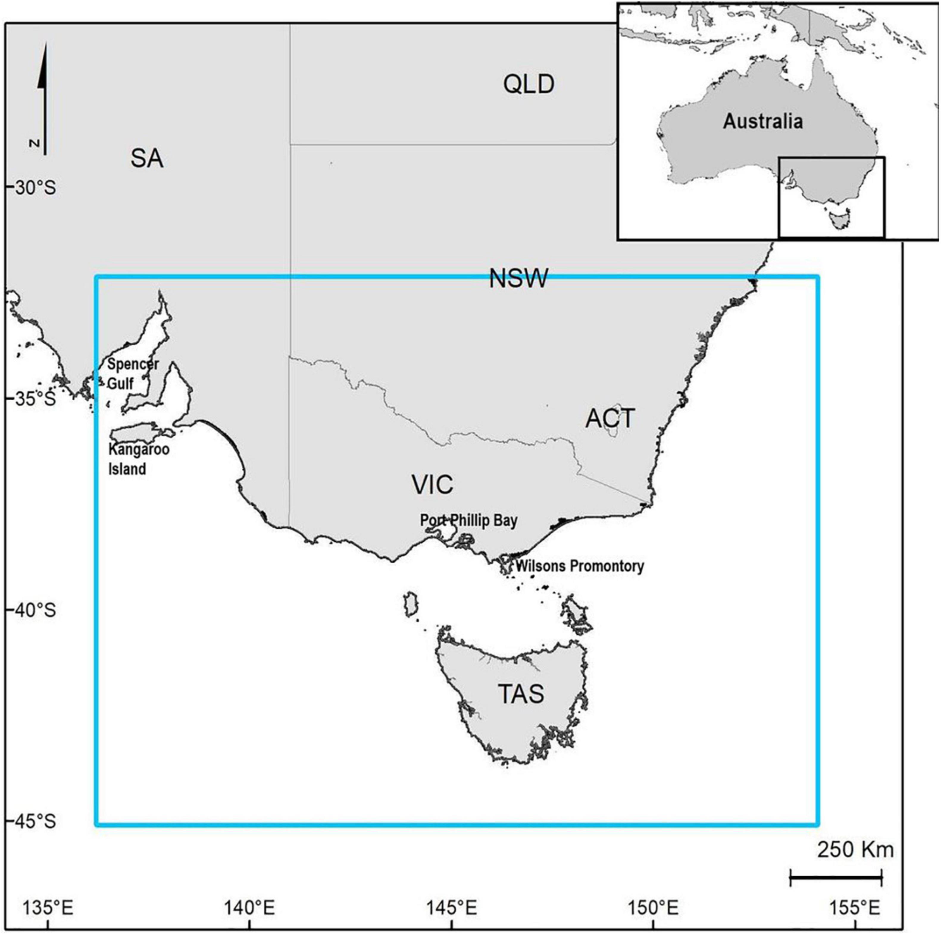
Figure 1. Map of the study area.
We identified habitat patches using data available through Seamap Australia National Benthic Habitat Classification Scheme (Butler et al., 2017). Data from this dataset were downloaded at state-resolution then merged. The extent of the study domain is 1,990 km × 1,850 km. We selected only habitats that are classified as rocky reefs contained in the domain area, and we aggregated habitat patches that showed a very limited size (of order of less of 1 km2) into a single patch, where possible. We defined 236 rocky reefs patches across the whole region for an extent of 15,248 km2 of available habitat for the sea urchin and 264,050 km2 for the snapper, which includes reefs surrounding area that could be used by this species.
Seascape Connectivity for Snapper (C. auratus)
To model adult snapper movements across the seascape and quantify habitat connectivity, we (1) built a cost surface layer based on magnitude and direction of oceanic currents, and (2) completed a least-cost path analysis to quantify seascape connectivity. The cost surface, required for the least cost path analysis (LCP), assumed fish movement was influenced by the magnitude and the direction of currents, with least cost following the direction of currents. Magnitude and direction of currents were derived from a global ocean circulation model (HYCOM)1 using the Marine Geospatial Ecology Toolbox, MGET (Roberts et al., 2010) in ArcGIS® 10.5.1 (ESRI, 2017). Data were aggregated into single annual cumulative cost layers, representative of currents magnitude and currents direction for the entire region (see Supplementary Figure 1). Following examples from terrestrial habitat, first we created two cost surfaces, one for currents’ magnitude and one currents’ direction, quantifying the increasing relative cost of moving across the seascape. Generally, due to the dominant eastward flow of currents, the cost of moving in this direction was less than traveling westward (Caldwell and Gergel, 2013). We reclassified both layers and assigned a relative score representing the cost of traveling (Rayfield et al., 2010), ranging from 1 to 10, with a score of 1 representing the least cost, while 10 represented the greatest cost of travel, ten times more costly compared to cells with a value of 1. Finally, we combined the currents magnitude and currents direction cost surfaces, calculating the weighted mean and defining one cumulative movement cost surface among all study area, assuming parameters have equal weight. See Supplementary Material for further details.
We performed LCP analysis using Linkage Mapper 2.0.0 (McRae and Kavanagh, 2011) a toolbox freely available for ArcGIS® 10.5.1 (ESRI, 2017). To add realism to the model, we applied a maximum threshold of 100 km of traveled distance, based on maximum swimming linear distances recorded from acoustic tagging of snapper in South-east Australia (Fowler et al., 2017). We modeled only ecologically meaningful corridors among all habitat patches within the swimming range of snappers. Our LCP analysis resulted in maps representing seascape connectivity for adult snapper, with routes showing the least costly paths among all habitat patches (nodes). This LCP network was used to further quantify the structure of seascape connectivity (see Supplementary Figure 3).
Seascape Connectivity for Purple Sea Urchin (H. erythrogramma)
For marine invertebrates such as H. erythrogramma, movements across the seascape are largely determined by the larval dispersal phase. We modeled larval connectivity using an existing spatially explicit biophysical marine connectivity model (Treml et al., 2012). In this model, we used (1) a map defining suitable rocky reef habitat patches, same data as above for snapper, where all the habitat patches are source and destination sites for larvae, (2) data describing the ocean currents (HYCOM), and (3) species-specific life history traits for H. erythrogramma (Supplementary Table 1), obtained from the literature (Okubo, 1971; Rumrill, 1987; Lamare and Barker, 1999; Huggett et al., 2008; Swanson et al., 2012; Williams and Hastings, 2013).
We simulated larval dispersal from 1992 to 2012 at a 3-hourly time-step, using all the available data for all spawning times. Clouds of larvae were released from source reef patches and the likelihood of larval settlement to all destination patches was estimated based on species-specific biological parameters and ocean characteristics. The model output was a dispersal matrix, recording the cumulative quantity of larvae released from each source patch that survived and settled to each destination patch, summarizing across all modeled dispersal events and years, and scaled by the size of the available habitat area. Migration matrices are commonly used to study larval connectivity, for this reason the dispersal matrices were converted to migration matrices, M, representing the proportion of settled larvae arriving at each destination (columns in the matrix) that came from each source patch (rows in the matrix). The migration matrix was used to build a network of seascape connectivity, where rocky reef patches correspond to graph nodes and presence of larval connectivity was represented as graph edges (Supplementary Figure 4).
Network Analysis and Spatial Generalization of Centrality Measures
The species-specific connectivity data were used to quantify patch-level metrics representing patch importance, a common spatial ecology approach (Estrada and Bodin, 2008; Bodin and Saura, 2010; Carroll et al., 2012). All metrics were calculated in R (R Core Team, 2019) with the “igraph” package (Csardi and Nepusz, 2006). For all patches, we calculated degree centrality, betweenness centrality and eigenvector centrality. Centrality metrics indicate how central a node is in a network, therefore a node with a high value of centrality is expected to have high habitat connectivity importance. Degree centrality is the number of outgoing and incoming links with each node in the network. Betweenness centrality is a measure based on shortest paths, and it is calculated as the number of shortest paths between all pairs of nodes in the graph that pass through that node (Freeman, 1978; Newman, 2005). Eigenvector centrality is a measure of importance of a node, essentially identifying highly connected nodes that are also connected to other highly connected nodes. Compared to other centrality metrics eigenvector centrality values are defined between 0 and 1, where a value of 1 is assigned to the most influential node in the network and 0 to the least influential. This metric assigns relative scores to all nodes in the network and is estimated as the principal eigenvector of the adjacency matrix defining the network (Borgatti, 2005).
Species distribution models require continuous explanatory variables, therefore we interpolated our centrality estimates across the seascape domain. The interpolation technique and distance used was dependent on each species’ capacity to move throughout the seascape. In the case of the purple sea urchin, with its limited ability to move great distances following settlement, centrality values were interpolated locally only and assigned to all habitat cells in the focal rocky reef patch. For the snapper we assigned the corresponding centrality value to each patch cell, and due to the likelihood of movement at greater distances, we extrapolated the centrality measure into the neighboring seascape using a negative exponential function with respect to distance. Consistent with the 100 km threshold used in the LCP analysis (Fowler et al., 2017), a maximum dispersal distance of 100 km corresponds to a probability of presence of p = 0.05 (Urban and Keitt, 2001; Foltête et al., 2012). We multiplied this probability by the centrality value of the habitat patch. Where values from two or more patches intersect, the mean centrality value was used in these intervening areas. The results are continuous centrality surfaces which can then be appropriately integrated into SDMs.
Species Distribution Modeling and Comparison of Models’ Performance
We developed SDMs for both species, including and excluding the species-specific centrality surfaces. Species occurrences data recorded inside our spatial domain were derived from the Atlas of Living Australia [ALA] (2019, 2020)2, and contained reliable occurrence data for species around Australia. Environmental parameters were extracted using the “Bio-Oracle” package in R, which contains many marine data layers for ecological modeling (Tyberghein et al., 2012). Given that ALA data cover a temporal period of more than 100 years, we cleaned the data set to remove the oldest data and duplicates to better align to the temporal extent of the environmental data. For both species we selected only data from 1980. The final presence data for purple sea urchin consists of 875 observations, distributed across the study area, with the largest concentration within Port Phillip Bay, while snapper occurrence data consists of 780 observations, distributed across Victoria, South Australia and northern Tasmania, reflecting the known habitat of this species.
We selected a group of ecologically important parameters which were believed to contribute to the distribution of both species. Temperature, chlorophyll A concentration, primary production (measured as net primary productivity of carbon), current velocity, dissolved oxygen data were summarized by the long-term monthly mean, pH, bathymetry, and salinity were downloaded from models or summarized in situ measurements (for additional information see Supplementary Material). In addition to these environmental data, we included the seascape connectivity layers of betweenness centrality, degree centrality and eigenvector centrality (Figure 2). Collinearity among predictors was quantitatively checked, and those with a Pearson correlation threshold of 0.7 or greater were identified and one was eliminated leaving the most ecologically meaningful parameter in the model. Collinearity is a known source of uncertainty, and when collinearity increases, the efficiency and statistical power of the model decrease (De Marco and Nóbrega, 2018).
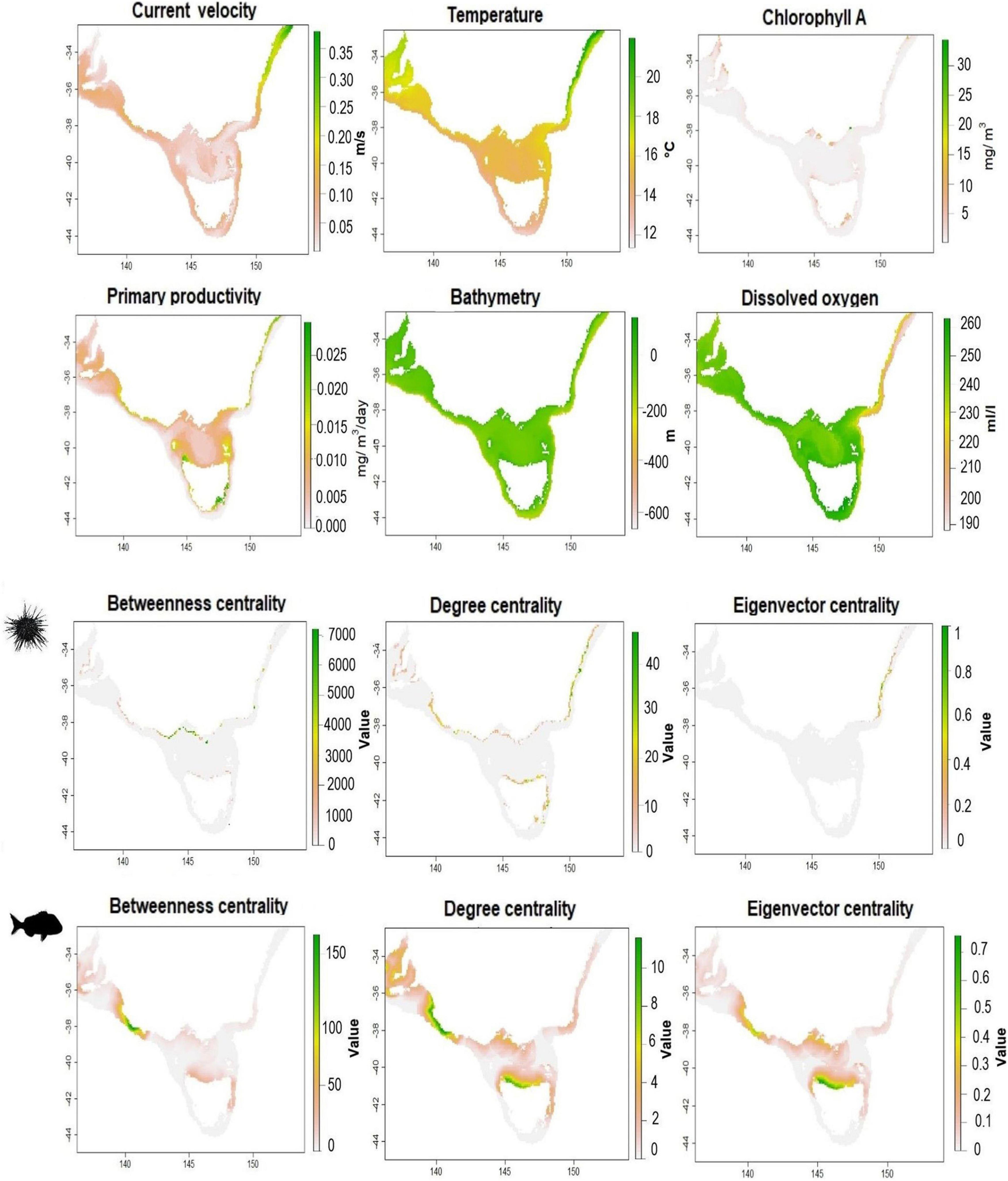
Figure 2. Maps of environmental and connectivity predictors used in the SDMs for purple sea urchin, H. erythrogramma (top), and snapper, C. auratus (bottom). All Maps in WGS84.
Among the many SDMs algorithms available, we used a popular machine learning method, boosted regression trees (BRT) (Elith et al., 2008). BRT is a form of logistical regression using decision trees and a boosting algorithm, an optimization technique that reduces predictive deviance by combining numerous trees into a single model. BRT has a powerful predictive performance and it has features such as handling different type of predictors, missing data, moderate collinearity, and complex non-linear relationships (Elith et al., 2008; Cimino et al., 2020). BRT also performs well for presence-only data (Elith et al., 2006). To model presence-only data with machine learning methods, a random sample of the background landscape is taken to represent unavailable “absence” data. In each model we defined 10,000 pseudo-absences, distributed equally across the coastal areas within the study area, representative of the potential species habitat. We followed the protocol for fitting BRT established within the “dismo” package (Hijmans et al., 2017) in R, to understand which was the best predictive model and compare the significance of including seascape connectivity in the models. We built a training dataset and a test dataset by resampling presence and background data, allocating them to cross validation (cv) folds. Evaluation was completed at two levels, first we used 10-folds to evaluate the models, then for each training fold a 5-folds internal cross validation procedure was completed for tuning the parameters of the BRT model using the “dismo” R package (Hijmans et al., 2020). Models’ settings (Table 1) were selected according to the recommendations in the literature (see Elith et al., 2008). The selected settings directly affect the number of optimal trees. As a result, by keeping the learning rate and tree complexity constant, we can optimize the number of trees to fit a good model. The settings were selected to aim for a model with a high number of trees, so the model can reliably estimate our response (Elith et al., 2008). We used cross-validation to evaluate the predictive power of the models and assessed performance using AUC-ROC, or area under the curve – receiver operating characteristics curve approaches. Then, we quantified the relative influence of seascape centrality metrics with respect to all other environmental variables to assess their contribution in predicting species distributions. We also quantified pairwise interactions between environmental and connectivity variables and environmental variables themselves, which is useful to define the most suitable environment for the species (Elith et al., 2008). BRT automatically models predictor interactions, allowing their magnitude, and therefore ranking, to be calculated (Hastie et al., 2009). Interaction results can be visualized as three-dimensional partial dependence plots.
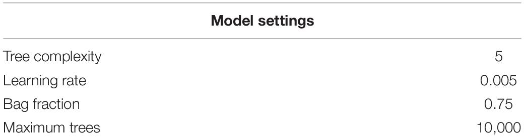
Table 1. Boosted regression trees settings applied to all models.
For each species we present results for two connectivity-enhanced models compared to a model without connectivity. First, we investigated the effect of connectivity adding to the model all centrality metrics (degree, betweenness, and eigenvector centrality) to understand which metric has the largest influence and we compared it to the model without centrality metrics. Then, to minimize overfitting and maximize predictive performance (Duan et al., 2014), we selected the single centrality metric with the largest relative influence in the model to remain in the model during fitting and we explored the SDMs results when we included or excluded connectivity. These additional models help to understand the role of connectivity and whether the SDM predictions were influenced by the number of connectivity parameters included in the model.
Finally, we mapped the spatial distribution of species across the study area to visualize and quantify differences in spatial predictions. To evaluate if there is a statistical relationship between centrality measures and models’ predictions, we tested them for correlation. Spatial indicators were used to quantify the differences in predicted habitat suitability from integrating connectivity or excluding connectivity. An overlay analysis was performed to identify areas within the SDM predictions that corresponded to critical connectivity areas revealed in the network analysis.
Results
Seascape Connectivity
We estimated seascape connectivity for both species (Supplementary Figures 2, 3) and no consistent spatial trend existed between species, revealing different connectivity structures across the seascape, according to species-specific dispersal characteristics. All centrality measures showed some spatial consistency within species, identifying similar areas of high and low values, revealing that hubs of connectivity (high degree centrality), populations stepping-stones (high betweenness centrality) and critical nodes (high eigenvector centrality) largely matched and were clustered in similar locations. Purple sea urchin showed well-connected areas, high eigenvector centrality and degree centrality, across north and east Tasmania, eastern Victoria, and New South Wales coast, while South Australia nodes had weak connections with the rest of the domain (Figure 2). Purple sea urchin stepping-stone habitats are clustered in central and eastern Victoria. Snapper connectivity revealed high values of centrality for patches along north of Tasmania and central Victoria coasts, while areas on the eastern and western boundaries of the domain, along South Australia and New South Wales coasts, showed less connectivity (Figure 2).
Species Distribution Modeling and Comparison of Models’ Performance
The final SDMs included mean sea water temperature, chlorophyll A concentration, primary production, bathymetry, dissolved oxygen concentration, current velocity and centrality measures (Supplementary Table 2). Salinity and pH were removed for both species, due to strong correlation with other environmental variables, specifically salinity was highly correlated with temperature while pH was highly correlated with temperature and current velocity. Note that centrality measures displayed low correlation with the environmental variables included in the models, although they displayed greater correlation between centrality metrics, especially for snapper (Supplementary Figures 4, 5).
The optimal models’ results are summarized in Table 2. For both species, SDMs used a tree complexity of 5, a learning rate of 0.005, bag fraction of 0.75, 5 folds for tuning and a maximum of 10,000 trees. The optimal model for sea urchin used 4,300 trees for the model integrating all centrality metrics, 4,700 trees for the model including degree centrality only and 5,700 for the model without centrality metrics. Models showed good predictive performance with same mean AUC score (0.95 ± 0.01) for all models (with all centrality metrics, degree centrality only and without connectivity). The optimal model for snapper used 4,000 trees for the model integrating centrality metrics, 3,300 trees when only degree centrality is included in the model and 3,200 trees when seascape connectivity was excluded. The mean AUC score was 0.91 ± 0.03 for the models including all centrality metrics and degree centrality only while it was slightly lower (0.90 ± 0.03) in the model without connectivity.
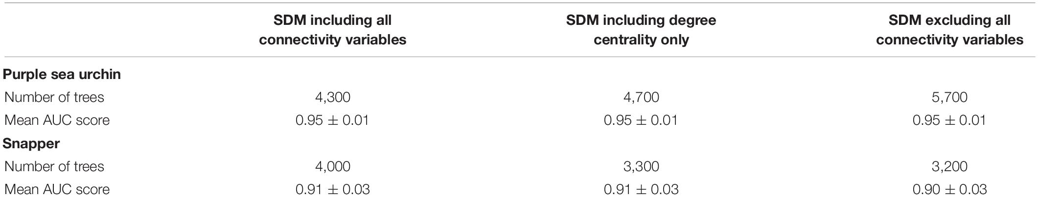
Table 2. Optimal SDMs models results for each species.
Environmental variables emerged as the most influential predictors for both species. For the sea urchin bathymetry showed the largest influence in all models, respectively, contributing between 25 and 30% to SDMs predictions, followed by temperature and dissolved oxygen which had a relative influence between 13 and 17% across the three sea urchin models (Figures 3A–C). Primary production, chlorophyll A and current velocity had a lower contribution, with relative influence varying between 7 and 15% (Figures 3A–C). For snapper, temperature was the most influential variable contributing between 36.5 and 40% to SDMs predictions in all the models (Figures 3D–F). Other environmental variables that showed an important relative influence for snapper were current velocity (13.2, 15.2, and 17.2%), followed by chlorophyll A (10.1, 11.6, and 13.3%). Dissolved oxygen, primary production and bathymetry were less influential with relative influence values varying from 7 to 11.5% (Figures 3D–F).
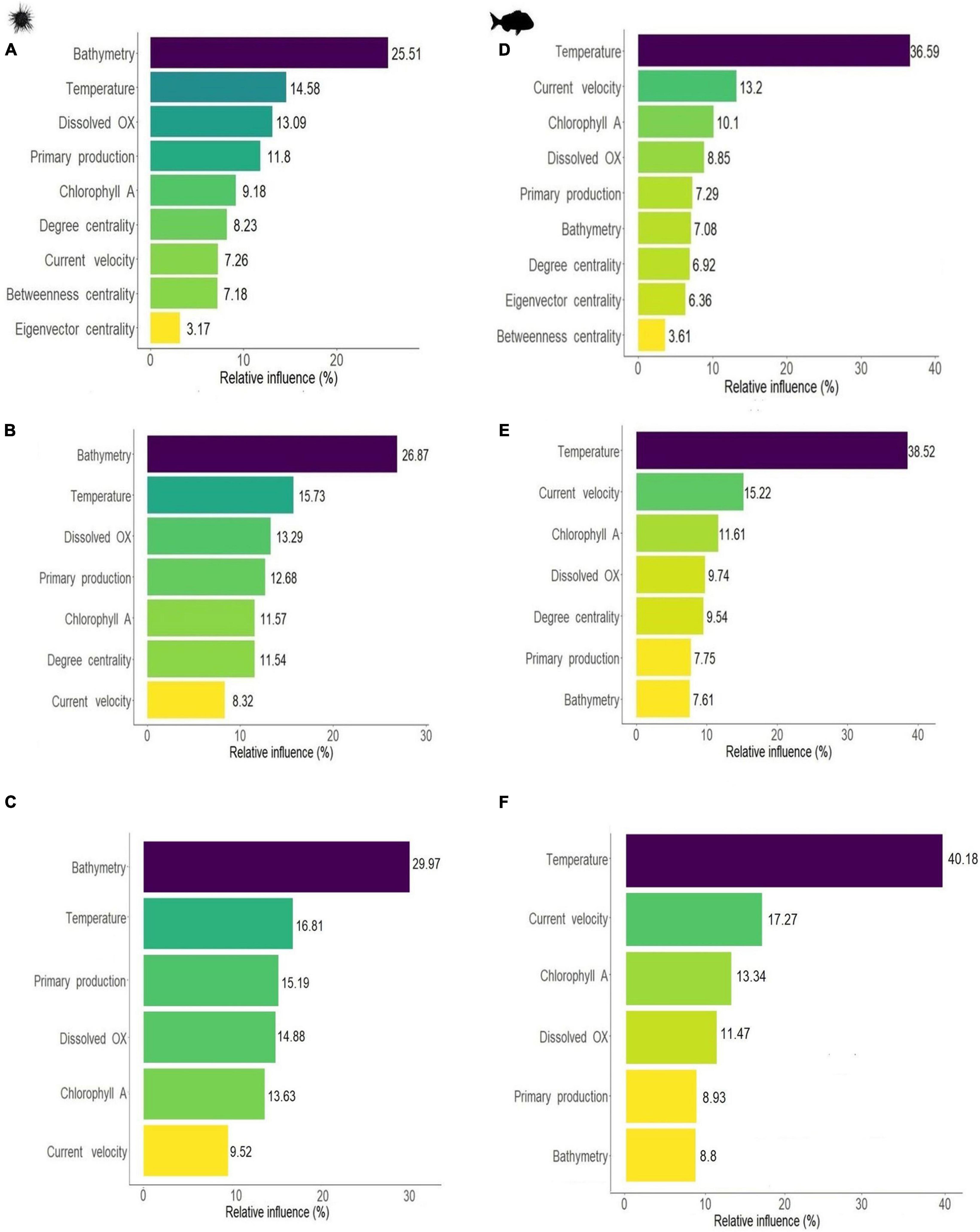
Figure 3. Relative influence of environmental parameters and centrality metrics on SDM results for sea urchin H. erythrogramma (left) and snapper, C. auratus (right). Fitting BRT including all centrality measures (A,D) or selecting only the most influential variable degree centrality (B,E), or excluding centrality (C,F). Relative influence expressed in percentage (i.e., total influence sums up to 100%).
Centrality measures had some influence across both species with degree centrality emerging as the most important centrality measure. For the purple sea urchin SDM, connectivity contributed to a total of 18.6% to the final model, with degree centrality having the largest relative influence (8.2%), followed by betweenness centrality (7.2%) and eigenvector centrality (3.2%) (Figure 3A). Degree centrality was more influential than current velocity (7.3%) and similar to chlorophyll A concentration (9.2%). Centrality measures showed pairwise interactions with several of the environmental variables (see three-dimensional dependence plots Supplementary Figures 7, 8). Eigenvector centrality had the strongest interactions with current velocity and primary production, degree centrality had interactions with primary production and bathymetry, while betweenness centrality interacted with temperature and bathymetry. For snapper, all centrality measures had a lower relative influence than the environmental parameters, and contributed at most 17% to SDM predictions. Degree centrality was the most influential among the centrality metrics, with a relative influence of 6.9%, followed by eigenvector centrality (6.4%) and betweenness centrality (3.6%) (Figure 3D). Centrality measures interacted with environmental variables, and the strongest interactions were with temperature for degree centrality and eigenvector centrality, and bathymetry for betweenness centrality (Supplementary Figures 7, 8).
We selected only the network-based metric with the largest influence to reduce the number of variables and increase the predictive power. Degree centrality was selected for both species, and we therefore compared the SDM results between models with and without degree centrality included (Table 2). Note that a lower number of predictors is expected to result in an overall increase in relative influence across all variables. In the purple sea urchin model, the relative influence of degree centrality was maintained among models, more influential than current velocity and similar to chlorophyll A concentration, primary production and dissolved oxygen (Figure 3B). For the sea urchin, the order of variables based on relative influence remained the same for the model including all centrality measures (e.g., Figures 3A vs. B), and degree centrality maintained a similar order of influence, comparable to chlorophyll A and well above the influence of current velocity. Degree centrality had some interactions with all the environmental parameters, but the strongest interactions were with bathymetry and high dissolved oxygen (Supplementary Figures 7, 8). In the snapper model the order of influence changed when only degree centrality was used, moving ahead of primary productivity and bathymetry in influence. The relative influence of degree centrality, when used as the sole connectivity metric moved in front of both primary productivity and bathymetry, and was comparable in influence to dissolved oxygen concentration (Figure 3E). Degree centrality interacted with all environmental variables, particularly with warm temperature and high bathymetry (Supplementary Figures 7, 8). Across all models and both species, connectivity metrics appeared to maintain a relative influence between 9.5 and 18.5% on species distributions.
We predicted species distribution and compared maps of habitat suitability, highlighting differences in species range (see Supplementary Figure 9 for habitat suitability predictions for all models). Despite these models predicted somewhat different species distribution range, when tested for pairwise correlation, the differences in spatial distribution showed very low correlation with the seascape centrality metrics for both species (Supplementary Figure 10).
The impact of including (or not) connectivity in the SDM predictions revealed geographic structure in terms of the magnitude of increase or decrease in modeled habitat suitability (Figure 4). For the purple sea urchin, most areas showed a decrease in habitat suitability when connectivity was included (i.e., these areas became less suitable in the model), particularly for Port Phillip Bay in Victoria and Spencer Gulf in South Australia and areas far from the coastline (Figure 4). Areas of increased habitat suitability were smaller and focused around “central” rocky reefs (Figure 4B). Located primarily around high degree centrality sites in central and western Victoria, north and east Tasmania and New South Wales (Figure 4A). Rocky reef patches with high betweenness centrality and eigenvector centrality did not correspond to key zones revealed from SDMs results (Supplementary Figure 11). Snapper habitat suitability predictions decreased for models including connectivity, especially for areas far from the coast. Areas associated to high degree centrality largely corresponded to higher suitability, particularly along north Tasmania, central Victoria and on the border between Victoria and New South Wales and South Australia habitats (Figure 4D). Areas of high eigenvector centrality in central Victoria and north Tasmania also correspond to high degree centrality, while there was no consistent spatial trend for betweenness centrality (Supplementary Figure 11).
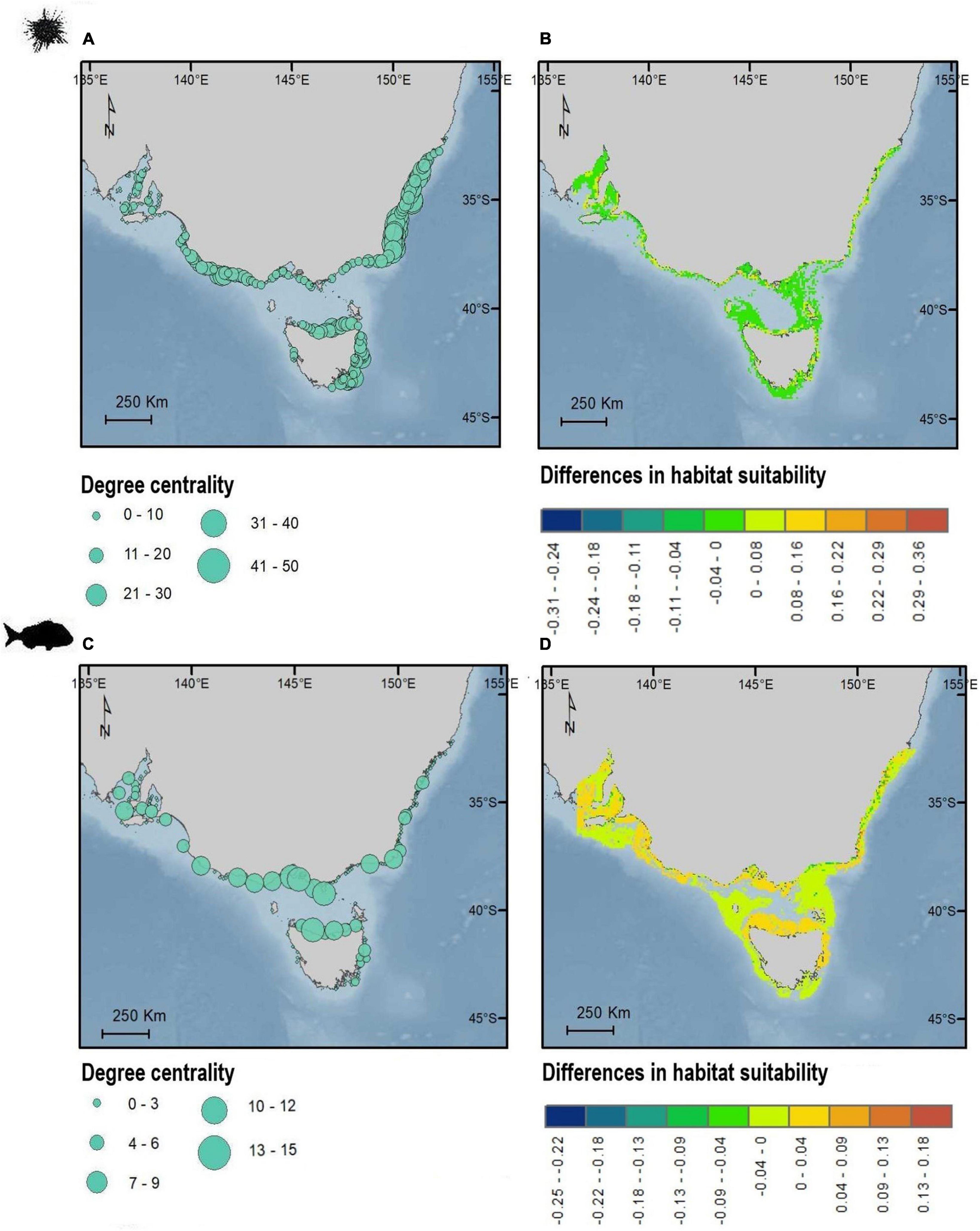
Figure 4. Maps showing the geographic distribution of degree centrality (A,C) and differences in spatial predictions of habitat suitability (B,D) for sea urchin H. erythrogramma (top) and snapper, C. auratus (bottom). Degree centrality (A,C) is shown as dots corresponding to the habitat patches centroids. Values of habitat suitability are positive when predicted habitat suitability is larger for SDM incorporating connectivity compared to the SDM without connectivity. Values of habitat suitability are negative when predicted habitat suitability is lower for SDM incorporating connectivity compared to the SDM without connectivity. Maps in WGS84.
Discussion
Seascape connectivity is essential for ensuring long term species persistence and determining the distribution of species (Engelhard et al., 2017; Weeks, 2017), and as a result is expected to have a significant influence on predicting species distribution with SDMs. Graph-based centrality metrics may influence SDMs predictions and degree centrality appeared to be the most important metric among the centrality measures.
Degree centrality was the most significant among the centrality measures included in the model. Degree centrality identifies hubs of high connectivity, and it is critically important for benthic species dispersing only during the larval stage, representing the quantity of larval connectivity, identifying important sources and destinations of larvae (Treml et al., 2015; Zamborain-Mason et al., 2017). Hotspots of connectivity ensure persistence in marine metapopulations (Zamborain-Mason et al., 2017; Cecino and Treml, 2021), and in this work was also significant in defining the species spatial distribution, showing that highly central nodes identified areas of greater habitat suitability. Connectivity variables had interactions with the environmental parameters revealing that the most suitable habitat also corresponded to critical habitats for connectivity. Quantifying interactions among variables helps to define more clearly which is the most suitable habitat for the species (Elith et al., 2008), showing how the effect of one environmental predictor on a species changes according to the levels of other predictors. Recognizing these environmental interactions is critical to assess changing environmental conditions, and integrating environmental and ecological interactions produces more robust SDMs and improves understanding of causes of species’ distributions (Guisan et al., 2006).
The results for degree centrality indicate that the sea urchin is predicted to occur in shallow waters, around high oxygen concentrations and in hubs of connectivity (degree centrality values between 10 and 20 ecological linkages). Both depth and connectivity are critical to define benthic species distribution, while dispersal largely influences the spatial distribution and range extension (Ling et al., 2009). Depth was found to influence reproduction in sea urchin, where higher gonad index was associated to individual occupying the intertidal zone compared to sea urchins living in the subtidal zone (Basch and Tegner, 2007). The role of temperature as an influential predictor of sea urchin distribution is particularly relevant to the management of sea urchin species due to their range expansion along with the tropicalization of south-eastern Australian waters and the consequential loss of kelp. Using mechanistic species distribution models, range shifts of sea urchins were predicted, revealing how these shifts are driven by climate, therefore leading to the contraction of habitat-forming species such as kelp (Castro et al., 2020).
Snapper, in contrast, is predicted to be found around hubs of connectivity (degree centrality of value 4 and 8), and in warm shallow waters. Elevated temperature is associated with increased larval size and survival influencing the snapper adult population dynamics (McMahon et al., 2020). Adult snapper movement appeared to concentrate around these warmer habitats, where conditions are optimal for larval rearing (Fielder et al., 2005). Current velocity emerged as another influential environmental parameter influencing the snapper SDMs (Figure 3). Current velocities proved to be critical to distinguish between juvenile and adult habitat for New Zealand snapper populations (Compton et al., 2012). Water column features such as currents largely influence species distribution predictions of south-east Australian nearshore temperate reef fishes, while other environmental variables like bathymetry appeared to be less important predictors (Young and Carr, 2015).
Machine learning methods such as BRT offer the advantage of exploring not only model performance but also the extent of each variable’s relative influence. If predictors have no contribution, the model algorithm calculates the relative variable influence as zero or near zero. In our species distribution models, connectivity contributes to the model, yet the influence on predictions was not as strong as key environmental variables, such as temperature, currents and chlorophyll. As a result, if centrality metrics were omitted, the resultant models would have resulted in different habitat suitability predictions, especially affecting their spatial range. When we included the most influential metric, degree centrality, the influence of connectivity on SDMs predictions increased together with the other predictors remaining among the least influential variables, however, its influence showed a larger increase compared to other environmental predictors. In both species the area under the curve (AUC-ROC) of the models was close to one, indicating that the model performance and predictions were very good (Jiménez-Valverde, 2012). AUC scores were similar for models with and without connectivity, suggesting no differences in the models’ predictive performance, however, the spatial range of habitat suitability predictions differed among the models, indicating that differences between the models exist. This apparent contradiction may be explained by the high accuracy typical of machine-learning algorithms (Bucklin et al., 2015). Independent to connectivity, the most influential environmental drivers were bathymetry and temperature for purple sea urchin, and temperature and current velocity for snapper (Figure 3), commonly found to have large influence across many marine-focused SDMs (Reiss et al., 2011; Tyberghein et al., 2012).
Despite the limited differences in habitat suitability magnitude, when incorporating connectivity in SDMs’ spatial predictions revealed reduced suitability primarily for deep waters, defining a more restricted geographic range for snapper and sea urchins, limiting the distributions to shallow coastal waters. In addition, the inclusion of connectivity in the SDMs increase to a small extent the suitability around several clusters of connectivity hubs. Habitats with high degree centrality, were identified in central Victoria, in proximity of Wilsons Promontory particularly for snapper population, key habitats for metapopulation persistence across species and corresponding to marine protected areas and reserves (Cecino and Treml, 2021). This region significance is well known and includes several ecological features, which define the structure of the coastal communities. Eastern Victoria was identified as potential biogeographic break for many taxa often associated with limits in species’ ranges and changes in community assemblages (Colton and Swearer, 2012). Habitat patches in northern Tasmania may also be essential for ensuring connectivity between Tasmania and Victoria coasts. In Eastern Tasmania, the oceanographic mixing zone where subantarctic water masses, driven by westerly winds, interact with eddies from the East Australian current, lead to enhanced productivity, and phytoplankton blooms and mass aggregations of coastal temperate taxa occur (Hosack and Dambacher, 2012; Dambacher et al., 2012; Commonwealth of Australia, 2015). Snapper’s hubs of connectivity in South Australia are also consistent with key habitat sites for the snapper fishery and for spawning grounds (Fowler and Jennings, 2003).
Both study species used for this work have somewhat limited dispersal ability, especially in relationship to the extent of the model domain. This choice of model domain was made to highlight an ecologically and economically important Australian seascape, and the influence of ocean dynamics and life histories. However, further research effort may be needed where species have extended home ranges, long-distance swimming capacity, or where dispersal periods extend for many weeks or months.
Applying SDMs to marine species can be particularly challenging. Challenges in understanding how species are distributed across space arise when comprehensive sampling is not possible, for example for species with high degree of niche specialization, and/or restricted range (Araujo and Guisan, 2006). Several issues are somewhat unique of the marine environment. For example, a strong spatial bias in data collection, since different effort is required to collect data in shallow waters compared to deep waters, and the widespread spatial-temporal bias in global satellite-derived ocean measurements, due to unpredicted or unusual atmospheric properties affecting the algorithm interpretation, and the lack of in situ data to use for tuning (Robinson et al., 2011, 2017). In our models, occurrence data collected from the Atlas of Living Australia include data from early 1900s, while environmental data were based on information collected from 2000 (see Supplementary Material for details) and the connectivity models used ocean current data for the period 1992–2012. This might result in an underestimation of the importance of connectivity and its influence on model predictions. Despite the large temporal extent of the ALA data sets the oldest data largely corresponded the distribution of occurrences recorded in recent years. However, we focused our analysis on a cleaned and reduced data set, reducing the temporal differences among species data, environmental predictors and centrality metrics. The lack of true absence data may be another limitation when developing SDMs, especially for marine species, where presence data sampling is biased toward coastal waters and areas near ports (Robinson et al., 2011). Though we addressed this limitation to some degree by choosing BRT methods, an appropriate procedure when working with species presence and pseudo-absence data (Cerasoli et al., 2017). We selected BRTs over presence-only methods such as Maxent because BRTs allow for better control and quantification of predictors interactions, allows appropriate model complexity and tunes model parameters with internal cross-validation. Moreover, the predictive performance of BRT are comparable to Maxent for predicting presence-only species data (Valavi et al., 2021). BRTs outperform other approaches like generalized linear and additive models, as well as combine many decision trees to improve model’s accuracy, include stochasticity, reducing variance and improving predicting performance (Cimino et al., 2020). That said, BRTs are often criticized for their tendency to overfit models. Other limitations common to SDMs include changes in habitat conditions due to climate change and human impacts, and attempting to predict species around range shifts. For exploited taxa like snapper, the distribution of fishing effort likely influences species distribution and presence/absence data. Our models could potentially be improved by including data on fishing pressure and environmental changes to producing more realistic spatial predictions.
Across two very different marine taxa, centrality measures proved to be appropriate and flexible proxies to describe seascape connectivity and can effectively identify hotspots and stepping-stones of connectivity. Using these patch-level metrics to describe seascape connectivity is an efficient way to incorporate connectivity information into marine-based SDMs. Centrality metrics proved to have a limited contribution to SDMs, yet they contribute to define the spatial distribution patterns and the most suitable habitat patches. Importantly, centrality metrics interact with other environmental predictors, highlight the suitability of habitats combining environmental and connectivity characteristics. Connectivity is fundamentally important for marine species and should be considered in models of species distribution or abundance. Our new methods chart a pathway forward for efficiently incorporating connectivity into marine-based SDMs and open the door for exploring the broader influence of dispersal and movement on species distributions.
Data Availability Statement
Publicly available datasets were analyzed in this study. This data can be found here: https://doi.org/10.26197/5e337e7061fa7, https://doi.org/10.26197/5d673e22c2429, https://www.hycom.org/, and https://www.bio-oracle.org/code.php.
Author Contributions
GC: conceptualization, methodology, formal analysis, data curation, investigation, visualization, and writing – original draft preparation. RV: methodology, formal analysis, and writing – review and editing. ET: supervision, conceptualization, software, resources, and writing – review and editing. All authors contributed to the article and approved the submitted version.
Funding
Funding was provided through a Melbourne Research Scholarship to GC.
Conflict of Interest
The authors declare that the research was conducted in the absence of any commercial or financial relationships that could be construed as a potential conflict of interest.
Publisher’s Note
All claims expressed in this article are solely those of the authors and do not necessarily represent those of their affiliated organizations, or those of the publisher, the editors and the reviewers. Any product that may be evaluated in this article, or claim that may be made by its manufacturer, is not guaranteed or endorsed by the publisher.
Acknowledgments
Simulations were completed on the University of Melbourne High Performance Computing cluster, Spartan. We thank the reviewers for their thoughtful comments and efforts toward improving our manuscript.
Supplementary Material
The Supplementary Material for this article can be found online at: https://www.frontiersin.org/articles/10.3389/fmars.2021.766915/full#supplementary-material
Footnotes
References
Adams, M. P., Saunders, M. I., Maxwell, P. S., Tuazon, D., Roelfsema, C. M., Callaghan, D. P., et al. (2016). Prioritizing localized management actions for seagrass conservation and restoration using a species distribution model. Aquat. Conserv. Mar. Freshw. Ecosyst. 26, 639–659. doi: 10.1002/aqc.2573
Agardy, M. T. (1994). Advances in marine conservation: the role of marine protected areas. Trends Ecol. Evol. 9, 267–270. doi: 10.1016/0169-5347(94)90297-6
Araujo, M. B., and Guisan, A. (2006). Five (or so) challenges for species distribution modelling. J. Biogeogr. 33, 1677–1688. doi: 10.1111/j.1365-2699.2006.01584.x
Atlas of Living Australia [ALA] (2019). Chrysophrys auratus Occurrence Data. ALA. doi: 10.26197/5d673e22c2429
Atlas of Living Australia [ALA] (2020). Heliocidaris erythrogramma Occurrence Data. ALA. doi: 10.26197/5e337e7061fa7
Báez, J. C., Olivero, J., Peteiro, C., Ferri-Yáñez, F., Garcia-Soto, C., and Real, R. (2010). Macro-environmental modelling of the current distribution of Undaria pinnatifida (Laminariales, Ochrophyta) in northern Iberia. Biol. Invas. 12, 2131–2139. doi: 10.1007/s10530-009-9614-1
Basch, L. V., and Tegner, M. J. (2007). Reproductive responses of purple sea urchin (Strongylocentrotus purpuratus) populations to environmental conditions across a coastal depth gradient. Bull. Mar. Sci. 81, 255–282.
Bax, N., and Williams, A. (2000). Habitat and Fisheries Productivity in the South East Fishery Ecosystem. Deakin West, ACT: Fisheries Research and Development Corporation.
Bode, M., Burrage, K., and Possingham, H. P. (2008). Using complex network metrics to predict the persistence of metapopulations with asymmetric connectivity patterns. Ecol. Model. 214, 201–209. doi: 10.1016/j.ecolmodel.2008.02.040
Bodin, O., and Norberg, J. (2007). A network approach for analyzing spatially structured populations in fragmented landscape. Landsc. Ecol. 22, 31–44. doi: 10.1007/s10980-006-9015-0
Bodin, Ö, and Saura, S. (2010). Ranking individual habitat patches as connectivity providers: integrating network analysis and patch removal experiments. Ecol. Model. 221, 2393–2405. doi: 10.1016/j.ecolmodel.2010.06.017
Borgatti, S. P. (2005). Centrality and network flow. Soc. Netw. 27, 55–71. doi: 10.1016/j.socnet.2004.11.008
Bucklin, D. N., Basille, M., Benscoter, A. M., Brandt, L. A., Mazzotti, F. J., Romañach, S. S., et al. (2015). Comparing species distribution models constructed with different subsets of environmental predictors. Divers. Distrib. 21, 23–35. doi: 10.1111/ddi.12247
Burgess, S. C., Nickols, K. J., Griesemer, C. D., Barnett, L. A., Dedrick, A. G., Satterthwaite, E. V., et al. (2014). Beyond connectivity: how empirical methods can quantify population persistence to improve marine protected-area design. Ecol. Appl. 24, 257–270. doi: 10.1890/13-0710.1
Butler, C., Proctor, R. D., Flukes, E. D., Walsh, P., Johnson, C. P., and Lucieer, V. D. (2017). Seamap Australia - A National Seafloor Habitat Classification Scheme. Hobart TAS: University of Tasmania.
Caldwell, I. R., and Gergel, S. E. (2013). Thresholds in seascape connectivity: influence of mobility, habitat distribution, and current strength on fish movement. Landsc. Ecol. 28, 1937–1948. doi: 10.1007/s10980-013-9930-9
Carroll, C., McRAE, B. H., and Brookes, A. (2012). Use of linkage mapping and centrality analysis across habitat gradients to conserve connectivity of gray wolf populations in western North America. Conserv. Biol. 26, 78–87. doi: 10.1111/j.1523-1739.2011.01753.x
Castro, L. C., Cetina-Heredia, P., Roughan, M., Dworjanyn, S., Thibaut, L., Chamberlain, M. A., et al. (2020). Combined mechanistic modelling predicts changes in species distribution and increased co-occurrence of a tropical urchin herbivore and a habitat-forming temperate kelp. Divers. Distrib. 26, 1211–1226. doi: 10.1111/ddi.13073
Cecino, G., and Treml, E. A. (2021). Local connections and the larval competency strongly influence marine metapopulation persistence. Ecol. Appl. 31:e02302. doi: 10.1002/eap.2302
Cerasoli, F., Iannella, M., D’Alessandro, P., and Biondi, M. (2017). Comparing pseudo-absences generation techniques in Boosted Regression Trees models for conservation purposes: a case study on amphibians in a protected area. PLoS One 12:e0187589. doi: 10.1371/journal.pone.0187589
Cimino, M. A., Santora, J. A., Schroeder, I., Sydeman, W., Jacox, M. G., Hazen, E. L., et al. (2020). Essential krill species habitat resolved by seasonal upwelling and ocean circulation models within the large marine ecosystem of the California current system. Ecography 43, 1536–1549. doi: 10.1111/ecog.05204
Clauzel, C., Girardet, X., and Foltête, J.-C. (2013). Impact assessment of a high-speed railway line on species distribution: application to the European tree frog (Hyla arborea) in Franche-Comté. J. Environ. Manage. 127, 125–134. doi: 10.1016/j.jenvman.2013.04.018
Colton, M. A., and Swearer, S. E. (2012). Locating faunal breaks in the nearshore fish assemblage of Victoria, Australia. Mar. Freshw. Res. 63, 218–231. doi: 10.1071/MF10322
Commonwealth of Australia (2015). South-East Marine Region Profle: A Description of the Ecosystems, Conservation Values and Uses of the South-East Marine Region. Canberra ACT: department of agriculture water and the environment.
Compton, T. J., Morrison, M. A., Leathwick, J. R., and Carbines, G. D. (2012). Ontogenetic habitat associations of a demersal fish species, Pagrus auratus, identified using boosted regression trees. Mar. Ecol. Prog. Ser. 462, 219–230. doi: 10.3354/meps09790
Cowen, R. K., and Sponaugle, S. (2009). Larval dispersal and marine population connectivity. Annu. Rev. Mar. Sci. 1, 443–466.
Csardi, G., and Nepusz, T. (2006). The igraph software package for complex network research. Inter J. Complex Syst. 1695, 1–9.
Dambacher, J. M., Hayes, K. R., Hosack, G. R., Lyne, V., Clifford, D., Dutra, L. X., et al. (2012). National Marine Ecological Indicators. Hobart, Tas: CSIRO Mathematics, Informatics and Statistics.
De Marco, P. J., and Nóbrega, C. C. (2018). Evaluating collinearity effects on species distribution models: an approach based on virtual species simulation. PLoS One 13:e0202403. doi: 10.1371/journal.pone.0202403
Duan, R.-Y., Kong, X.-Q., Huang, M.-Y., Fan, W.-Y., and Wang, Z.-G. (2014). The predictive performance and stability of six species distribution models. PLoS One 9:e112764. doi: 10.1371/journal.pone.0112764
Elith, J., Graham, C. H., Anderson, R. P., Dudik, M., Ferrier, S., Guisan, A., et al. (2006). Novel methods improve prediction of species’ distributions from occurrence data. Ecography 29, 129–151. doi: 10.1111/j.2006.0906-7590.04596.x
Elith, J., and Leathwick, J. R. (2009). Species distribution models: ecological explanation and prediction across space and time. Annu. Rev. Ecol. Evol. Syst. 40, 677–697. doi: 10.1146/annurev.ecolsys.110308.120159
Elith, J., Leathwick, J. R., and Hastie, T. (2008). A working guide to boosted regression trees. J. Anim. Ecol. 77, 802–813. doi: 10.1111/j.1365-2656.2008.01390.x
Engelhard, S. L., Huijbers, C. M., Stewart-Koster, B., Olds, A. D., Schlacher, T. A., and Connolly, R. M. (2017). Prioritising seascape connectivity in conservation using network analysis. J. Appl. Ecol. 54, 1130–1141.
Estrada, E., and Bodin, O. (2008). Using network centrality measures to manage landscape connectivity. Ecol. Appl. 18, 1810–1825. doi: 10.1890/07-1419.1
Fielder, D. S., Bardsley, W. J., Allan, G. L., and Pankhurst, P. M. (2005). The effects of salinity and temperature on growth and survival of Australian snapper, Pagrus auratus larvae. Aquaculture 250, 201–214. doi: 10.1016/j.aquaculture.2005.04.045
Fischer, J., Kleidon, A., and Dittrich, P. (2015). Thermodynamics of random reaction networks. PLoS One 10:e0117312. doi: 10.1371/journal.pone.0117312
Foltête, J. C., Clauzel, C., Vuidel, G., and Tournant, P. (2012). Integrating graph-based connectivity metrics into species distribution models. Landsc. Ecol. 27, 557–569. doi: 10.1007/s10980-012-9709-4
Fowler, A., Huveneers, C., and Lloyd, M. (2017). Insights into movement behaviour of snapper (Chrysophrys auratus, Sparidae) from a large acoustic array. Mar. Freshw. Res. 68, 1438–1453. doi: 10.1071/MF16121
Fowler, A. J., and Jennings, P. R. (2003). Dynamics in 0+ recruitment and early life history for snapper (Pagrus auratus, Sparidae) in South Australia. Mar. Freshw. Res. 54, 941–956. doi: 10.1071/MF02172
Freeman, L. C. (1978). Centrality in social networks conceptual clarification. Soc. Netw. 1, 215–239. doi: 10.1016/0378-8733(78)90021-7
Girardet, X., Foltete, J. C., and Clauzel, C. (2013). Designing a graph-based approach to landscape ecological assessment of linear infrastructures. Environ. Impact Assess. Rev. 42, 10–17. doi: 10.1016/J.EIAR.2013.03.004
Gormley, K. S., Hull, A. D., Porter, J. S., Bell, M. C., and Sanderson, W. G. (2015). Adaptive management, international co-operation and planning for marine conservation hotspots in a changing climate. Mar. Policy 53, 54–66. doi: 10.1016/j.marpol.2014.11.017
Grober-Dunsmore, R., Pittman, S. J., Caldow, C., Kendall, M. S., and Frazer, T. K. (2009). “A landscape ecology approach for the study of ecological connectivity across tropical marine seascapes,” in Ecological Connectivity Among Tropical Coastal Ecosystems, ed. I. Nagelkerken (New York, NY: Springer), 493–530.
Guisan, A., Lehmann, A., Ferrier, S., Austin, M., Overton, J. M. C., Aspinall, R., et al. (2006). Making better biogeographical predictions of species’ distributions. J. Appl. Ecol. 43, 386–392. doi: 10.1111/j.1365-2664.2006.01164.x
Hamer, P. A., Acevedo, S., Jenkins, G. P., and Newman, A. (2011). Connectivity of a large embayment and coastal fishery: spawning aggregations in one bay source local and broad-scale fishery replenishment. J. Fish Biol. 78, 1090–1109. doi: 10.1111/j.1095-8649.2011.02921.x
Harasti, D., Lee, K. A., Gallen, C., Hughes, J. M., and Stewart, J. (2015). Movements, home range and site fidelity of snapper (Chrysophrys auratus) within a temperate marine protected area. PLoS One 10:e0142454. doi: 10.1371/journal.pone.0142454
Hastie, T., Tibshirani, R., and Friedman, J. (2009). The Elements of Statistical Learning: Data Mining, Inference, and Prediction, 2nd Edn. New York, NY: Springer series in statistics.
Hijmans, R. J., Phillips, S., Leathwick, J., and Elith, J. (2020). dismo: Specie Distribution Modeling. R package version 1.3-3. Available online at: https://CRAN.R-project.org/package=dismo (accessed October 11, 2021).
Hijmans, R. J., Phillips, S., Leathwick, J., Elith, J., and Hijmans, M. R. J. (2017). Package ‘dismo’. Circles 9, 1–68.
Hosack, G., and Dambacher, J. (2012). Ecological Indicators for the Exclusive Economic Zone of Australia’s South East Marine Region. CSIRO;2012. Canberra, ACT: CSIRO, doi: 10.4225/08/584c44e1a4389
Huggett, M. J., Crocetti, G. R., Kjelleberg, S., and Steinberg, P. D. (2008). Recruitment of the sea urchin Heliocidaris erythrogramma and the distribution and abundance of inducing bacteria in the field. Aquat. Microb. Ecol. 53, 161–171. doi: 10.3354/AME01239
Jiménez-Valverde, A. (2012). Insights into the area under the receiver operating characteristic curve (AUC) as a discrimination measure in species distribution modelling. Glob. Ecol. Biogeogr. 21, 498–507. doi: 10.1111/J.1466-8238.2011.00683.X
Jones, M. C., and Cheung, W. W. (2015). Multi-model ensemble projections of climate change effects on global marine biodiversity. ICES J. Mar. Sci. 72, 741–752. doi: 10.1093/icesjms/fsu172
Lamare, M. D., and Barker, M. F. (1999). In situ estimates of larval development and mortality in the New Zealand sea urchin Evechinus chloroticus (Echinodermata : Echinoidea). Mar. Ecol. Prog. Ser. 180, 197–211. doi: 10.3354/meps180197
Ling, S., Ibbott, S., and Sanderson, J. (2010). Recovery of canopy-forming macroalgae following removal of the enigmatic grazing sea urchin Heliocidaris erythrogramma. J. Exp. Mar. Biol. Ecol. 395, 135–146. doi: 10.1016/j.jembe.2010.08.027
Ling, S., Scheibling, R., Rassweiler, A., Johnson, C., Shears, N., Connell, S., et al. (2015). Global regime shift dynamics of catastrophic sea urchin overgrazing. Philos. Trans. R. Soc. B Biol. Sci. 370:20130269. doi: 10.1098/rstb.2013.0269
Ling, S. D., Johnson, C. R., Ridgway, K., Hobday, A. J., and Haddon, M. (2009). Climate-driven range extension of a sea urchin: inferring future trends by analysis of recent population dynamics. Glob. Change Biol. 15, 719–731. doi: 10.1111/j.1365-2486.2008.01734.x
McMahon, S. J., Parsons, D. M., Donelson, J. M., Pether, S. M., and Munday, P. L. (2020). Elevated temperature and CO2 have positive effects on the growth and survival of larval Australasian snapper. Mar. Environ. Res. 161:105054. doi: 10.1016/j.marenvres.2020.105054
McRae, B. H., and Kavanagh, D. M. (2011). Linkage Mapper Connectivity Analysis Software. Arlington, TX: The Nature Conservancy.
Meyer, C. G., Papastamatiou, Y. P., and Clark, T. B. (2010). Differential movement patterns and site fidelity among trophic groups of reef fishes in a Hawaiian marine protected area. Mar. Biol. 157, 1499–1511. doi: 10.1007/s00227-010-1424-6
Minor, E. S., and Urban, D. L. (2007). Graph theory as a proxy for spatially explicit population models in conservation planning. Ecol. Appl. 17, 1771–1782. doi: 10.1890/06-1073.1
Monk, J., Ierodiaconou, D., Versace, V. L., Bellgrove, A., Harvey, E., Rattray, A., et al. (2010). Habitat suitability for marine fishes using presence-only modelling and multibeam sonar. Mar. Ecol. Prog. Ser. 420, 157–174. doi: 10.3354/meps08858
Newman, M. E. (2005). A measure of betweenness centrality based on random walks. Soc. Netw. 27, 39–54. doi: 10.1016/j.socnet.2004.11.009
O’Hara, T. (2002). Endemism, rarity and vulnerability of marine species along a temperate coastline. Invertebr. Syst. 16, 671–684. doi: 10.1071/IT01034
Okubo, A. (1971). Oceanic Diffusion Diagrams. Deep-Sea Research 18, 789–802. doi: 10.1016/0011-7471(71)90046-5
Pearson, R. G. (2007). Species’ distribution modeling for conservation educators and practitioners synthesis. Am. Museum Nat. Hist. 50, 54–89.
Pederson, H. G., and Johnson, C. R. (2006). Predation of the sea urchin Heliocidaris erythrogramma by rock lobsters (Jasus edwardsii) in no-take marine reserves. J. Exp. Mar. Biol. Ecol. 336, 120–134. doi: 10.1016/j.jembe.2006.04.010
R Core Team (2019). R: A Language and Environment for Statistical Computing. Vienna: R Foundation for Statistical Computing.
Rayfield, B., Fortin, M.-J., and Fall, A. (2010). The sensitivity of least-cost habitat graphs to relative cost surface values. Landsc. Ecol. 25, 519–532. doi: 10.1007/s10980-009-9436-7
Reiss, H., Cunze, S., König, K., Neumann, H., and Kröncke, I. (2011). Species distribution modelling of marine benthos: a North Sea case study. Mar. Ecol. Prog. Ser. 442, 71–86. doi: 10.3354/meps09391
Roberts, J. J., Best, B. D., Dunn, D. C., Treml, E. A., and Halpin, P. N. (2010). Marine geospatial ecology tools: an integrated framework for ecological geoprocessing with ArcGIS, Python, R, MATLAB, and C++. Environ. Model. Softw. 25, 1197–1207. doi: 10.1016/j.envsoft.2010.03.029
Robinson, L., Elith, J., Hobday, A., Pearson, R., Kendall, B., Possingham, H., et al. (2011). Pushing the limits in marine species distribution modelling: lessons from the land present challenges and opportunities. Glob. Ecol. Biogeogr. 20, 789–802. doi: 10.1111/j.1466-8238.2010.00636.x
Robinson, N. M., Nelson, W. A., Costello, M. J., Sutherland, J. E., and Lundquist, C. J. (2017). A systematic review of marine-based species distribution models (SDMs) with recommendations for best practice. Front. Mar. Sci. 4:421. doi: 10.3389/fmars.2017.00421
Rose, K. A., Cowan, J. H. Jr., Winemiller, K. O., Myers, R. A., and Hilborn, R. (2001). Compensatory density dependence in fish populations: importance, controversy, understanding and prognosis. Fish Fish. 2, 293–327. doi: 10.1046/j.1467-2960.2001.00056.x
Rumrill, S. S. (1987). Differential Predation Upon Embryos and Larvae of Temperate Pacific Echinoderms. Edmonton, AB: University of Alberta.
Swanson, R. L., Byrne, M., Prowse, T. A. A., Mos, B., Dworjanyn, S. A., and Steinberg, P. D. (2012). Dissolved histamine: a potential habitat marker promoting settlement and metamorphosis in sea urchin larvae. Mar. Biol. 159, 915–925. doi: 10.1007/s00227-011-1869-2
Tarabon, S., Bergès, L., Dutoit, T., and Isselin-Nondedeu, F. (2019). Environmental impact assessment of development projects improved by merging species distribution and habitat connectivity modelling. J. Environ. Manage. 241, 439–449. doi: 10.1016/j.jenvman.2019.02.031
Terres, M. A., Lawrence, E., Hosack, G. R., Haywood, M. D., and Babcock, R. C. (2015). Assessing habitat use by Snapper (Chrysophrys auratus) from baited underwater video data in a coastal marine park. PLoS One 10:e0136799. doi: 10.1371/journal.pone.0136799
Treml, E. A., Ford, J. R., Black, K. P., and Swearer, S. E. (2015). Identifying the key biophysical drivers, connectivity outcomes, and metapopulation consequences of larval dispersal in the sea. Mov. Ecol. 3:16. doi: 10.1186/s40462-015-0045-6
Treml, E. A., Halpin, P. N., Urban, D. L., and Pratson, L. F. (2008). Modeling population connectivity by ocean currents, a graph-theoretic approach for marine conservation. Landsc. Ecol. 23, 19–36. doi: 10.1007/s10980-007-9138-y
Treml, E. A., Roberts, J. J., Chao, Y., Halpin, P. N., Possingham, H. P., and Riginos, C. (2012). Reproductive output and duration of the pelagic larval stage determine seascape-wide connectivity of marine populations. Integr. Comp. Biol. 52, 525–537. doi: 10.1093/icb/ics101
Tyberghein, L., Verbruggen, H., Pauly, K., Troupin, C., Mineur, F., and De Clerck, O. (2012). Bio-ORACLE: a global environmental dataset for marine species distribution modelling. Glob. Ecol. Biogeogr. 21, 272–281. doi: 10.1111/j.1466-8238.2011.00656.x
Urban, D., and Keitt, T. (2001). Landscape connectivity: A graph-theoretic perspective. Ecology 82, 1205–1218.
Valavi, R., Guillera-Arroita, G., Lahoz-Monfort, J. J., and Elith, J. (2021). Predictive performance of presence-only species distribution models: a benchmark study with reproducible code. Ecol. Monogr. e1486. doi: 10.1002/ecm.1486
Vanderklift, M. A., and Kendrick, G. A. (2004). Variation in abundances of herbivorous invertebrates in temperate subtidal rocky reef habitats. Mar. Freshw. Res. 55, 93–103. doi: 10.1071/MF03057
Watson, J. R., Siegel, D. A., Kendall, B. E., Mitarai, S., Rassweiller, A., and Gaines, S. D. (2011). Identifying critical regions in small-world marine metapopulations. Proc. Natl. Acad. Sci. U.S.A. 108, E907–E913. doi: 10.1073/pnas.1111461108
Weeks, R. (2017). Incorporating seascape connectivity in conservation prioritisation. PLoS One 12:16. doi: 10.1371/journal.pone.0182396
Williams, P. D., and Hastings, A. (2013). Stochastic dispersal and population persistence in marine organisms. Am. Natural. 182, 271–282.
Young, M., and Carr, M. H. (2015). Application of species distribution models to explain and predict the distribution, abundance and assemblage structure of nearshore temperate reef fishes. Divers. Distrib. 21, 1428–1440. doi: 10.1111/ddi.12378
Keywords: centrality measures, fragmented habitat, graph theory, machine learning, predictive model, seascape connectivity
Citation: Cecino G, Valavi R and Treml EA (2021) Testing the Influence of Seascape Connectivity on Marine-Based Species Distribution Models. Front. Mar. Sci. 8:766915. doi: 10.3389/fmars.2021.766915
Received: 30 August 2021; Accepted: 24 November 2021;
Published: 14 December 2021.
Edited by:
Mark J. Henderson, United States Geological Survey, United StatesReviewed by:
Xiaolong Yang, National Marine Environmental Monitoring Center, ChinaVera Rullens, University of Waikato, New Zealand
Copyright © 2021 Cecino, Valavi and Treml. This is an open-access article distributed under the terms of the Creative Commons Attribution License (CC BY). The use, distribution or reproduction in other forums is permitted, provided the original author(s) and the copyright owner(s) are credited and that the original publication in this journal is cited, in accordance with accepted academic practice. No use, distribution or reproduction is permitted which does not comply with these terms.
*Correspondence: Giorgia Cecino, Z2lvcmdpYS5jZWNpbm9AZmF0aG9tcGFjaWZpYy5jb20=
†Present address: Giorgia Cecino, Fathom Pacific Pty Ltd., Melbourne, VIC, Australia