Interannual Abundance Fluctuations of Two Oceanic Squids in the Pacific Ocean Can Be Evaluated Through Their Habitat Temperature Variabilities

Introduction

Ommastrephid squids are economically imperative targets in the global distant-water fisheries (Arkhipkin et al., 2015b). Annual catches of Ommastrephid squids in the 2000s were over 2 million tons and accounted for over 50% of the total catches of cephalopod in the world (Chen et al., 2008). In the Pacific Ocean, neon flying squid (Ommastrephes bartramii) and jumbo flying squid (Dosidicus gigas) are the primary targets of Chinese Squid-jigging fleets. Within 2010∼2019, mean catches of O. bartramii and D. gigas were 41136.40 and 274442.89 tons, respectively. O. bartramii and D. gigas have become the most essential squid targets in the Pacific Ocean, accounting for 20∼40% of the yearly Chinese cephalopod catches during the 2010s. However, the catches had high fluctuations over years.

Ommastrephes bartramii (O. bartramii) and Dosidicus gigas (D. gigas) play crucial roles in the pelagic ecosystem (Markaida and Sosa-Nishizaki, 2003; Kumar et al., 2014). The spatial and temporal variations of O. bartramii and D. gigas and their association with the ocean environment are hot topics because they are highly migratory species and have large fluctuations in abundance. Previous studies can be divided into two parts: small scale and large scale. At the small scale, studies focused on the seasonal (intra-annual) variations (abundance and distribution) of the squids’ fishing ground and its relationship with environmental parameters derived from satellite remote-sensing data [such as seawater temperature (SST), sea surface height (SSH), sea surface salinity (SSS), chlorophyll-a (Chl-a), and sea level anomaly (SLA), Taipe et al., 2001; Paulino et al., 2016; Yu et al., 2016a, 2017b, 2019; Liu et al., 2017; Feng et al., 2018]. Specifically, the habitat models [such as habitat index model (HSI) and maximum entropy model (MaxEnt)] are widely used to simulate the spatial distribution of O. bartramii and D. gigas and explain seasonal (intra-annual) variations of abundance by combining with environmental parameters (Chen et al., 2010; Alabia et al., 2015a,b; Yu et al., 2019). To summarize, the distribution and abundance are extremely sensitive to the dynamics of oceanographic features (such as temperature, feeding conditions, and oceanic mesoscale processes) derived from the environment parameters. Among all the environmental parameters, SST is believed to be the most important factor (Alabia et al., 2015b).

At the large scale, the annual and interannual abundance and habitat fluctuations of O. bartramii and D. gigas and their association with the environment or climate variabilities are investigated. A recent issue is the mechanisms of their recruitment formation. The abundance of O. bartramii and D. gigas, which are the short-lived species (O’Dor, 1998; Ichii et al., 2009; Arkhipkin et al., 2015b), is considered to be greatly affected by the environment-induced recruitment dynamics in 1 year (Yatsu et al., 2000; Ichii et al., 2002; Chen et al., 2007; Cao et al., 2009). Previous studies suggested that the recruitment dynamics of O. bartramii could be related to the proportion of favorable SST areas (Chen et al., 2007), food conditions (Ichii et al., 2011; Nishikawa et al., 2014), and physical ocean processes (Nishikawa et al., 2015; Igarashi et al., 2017; Yu et al., 2017a,b) at its spawning ground. Concerning D. gigas, Waluda and Rodhouse (2006) reported that the favorable SST for hatching and development was 24∼28°C. Many studies confirmed that the SST can be the most imperative one affecting the entire life history dynamics of O. bartramii and D. gigas (Yatsu et al., 2000; Ichii et al., 2009; Yu et al., 2021a).

Since O. bartramii and D. gigas are regarded as major commercial squid fisheries in the Pacific Ocean, their annual and interannual abundance fluctuations are of high concern to many researchers. One question can be summarized as the mechanisms of abundance fluctuations under the middle- or large-scale climate variabilities [such as El Niño and La Niña and the Pacific Decadal Oscillation (PDO)]. Many studies reported the internal or indirect links in which the climate variabilities can affect annual and interannual abundance fluctuations of O. bartramii and D. gigas through the small-scale/local environment changes at the habitat (Yatsu et al., 2000; Taipe et al., 2001; Waluda et al., 2006; Chen et al., 2007; Yu et al., 2016a,b,c; Ichii et al., 2009, 2011; Igarashi et al., 2017; Yu and Chen, 2018). The other complication is the annual and interannual variabilities of the stock abundance, which is the basis of scientific study and rational fishery management. The O. bartramii and D. gigas are currently regulated and monitored by the North Pacific Fisheries Commission (NPFC) and South Pacific Regional Fisheries Management Organization (SPRFMO), respectively. Some studies supported stock assessment results for these two squids as the references in management (Ichii et al., 2006; Wang et al., 2016; Xu et al., 2017; Cordue et al., 2018). Nevertheless, Arkhipkin et al. (2020) summarized that the difficulties of the stock assessment and management of cephalopods species are their unique life history characteristics such as short life spans and semelparous reproduction, high natural mortality rates, rapid and often no asymptotic growth, and complex population structures. Furthermore, Arkhipkin et al. (2020) recommended that the depletion model should be applied in the stock assessment of cephalopods. In this way, the in-season catch and catch per unit effort (CPUE) times series are focused, and the fast dynamics of cephalopod life histories could be captured. In short, the small-scale/local environment changes cannot be neglected in the studies of the annual and interannual abundance fluctuations for O. bartramii and D. gigas.

Nonetheless, focusing on the abundance dynamics at the large-scale studies is also important because they can expand the perspectives to the long-term changes of marine species and ecosystems (so-called regime shift). Studies of the stock of the autumn cohort of O. bartramii revealed that its abundance was at a very low level before 1992 and thereafter increased (Yatsu et al., 2000; Ichii et al., 2009). The high/low-level periods correspond to a well-documented regime shift in the Pacific Ocean: anchovy- and sardine-dominant ecosystem (Chavez et al., 2003). Regarding D. gigas, individuals in Peruvian waters can be distinguished to three phenotypic groups (small, middle, and large) based on maximum body size and the size at which they reach sexual maturity (Argüelles et al., 2008). Argüelles et al. (2019) suggested that the predominance of three phenotypic groups at different times could be used as the indicator of regime shift in Peruvian waters (for example, 1989∼1999: a warmer period, a phenotypic group that matures at small- and medium-size predominant and 2000∼2016: A colder period, a phenotypic group that matures at large size predominant). Specifically, because these two squids are the major targets of Chinese squid-jigging fleets concurrently in the Pacific Ocean and can be caught at the same month in 1 year, Chinese fishery enterprises need to assign fishing efforts (the number of fishing vessels that should be distributed for these two squids) based on which squid is more abundant (Yu et al., 2021a). Yu et al. (2021a) demonstrated synchronous variations in abundance and distribution between O. bartramii and D. gigas from September to November during 2006∼2015, as well as a significant negative relationship in the abundance between these two squids because the proportion of favorable-SST area conversely shifts due to the SST anomaly changes at Niño 3.4 and Niño 1 + 2 regions. In addition, Yu et al. (2021b) investigated the habitat differences of O. bartramii and D. gigas between warm and cold PDO phases. They revealed that the changes in the PDO-induced opposite suitable habitat area would lead to the alternate shift of their abundance.

The results of Yu et al. (2021a,b) were based on the seasonal (September to November) instead of the all-year fishery data. However, the analysis based on the all-year fishery data can promote a better understanding for the mechanisms of the annual and interannual abundance fluctuations under small- and large-scale environmental or climate variabilities. This can also ensure the ration and suitable management of these two squids and provide a reference for the research on the role of squids in the marine ecosystem regime shift. In this study, annual and interannual abundance fluctuations of O. bartramii and D. gigas within 2003∼2020 are investigated based on the historical Chinese Squid-jigging fleets operation data. The study focuses on the stock of the western winter-spring cohort of O. bartramii (captured at the western water of 170°E) and the group of D. gigas off Peru Exclusive Economic Zone (PEEZ) waters. The stock/group studied is the main fishing target of O. bartramii and D. gigas by Chinese Squid-jigging fleets. Specifically, the Hodrick—Prescott filter analysis (Hodrick and Prescott, 1997) is used to quantify the annual and interannual abundance fluctuations since the annual abundance fluctuations had large variations.

Previous studies demonstrated that (1) the temperature (SST) is the most crucial environmental factor in the life histories of O. bartramii and D. gigas and (2) climate variabilities (especially, El Niño and La Niña and PDO) can affect annual and interannual abundance fluctuations of O. bartramii and D. gigas through the small-scale/local environmental changes at the habitat. In this study, annual and interannual abundance fluctuations associated with habitat temperature variabilities are examined. The habitat temperature variabilities are defined as the effective principal components of the SST at the squids’ two essential habitats (spawning and feeding ground) through life histories according to the principal component analysis (PCA, Venables and Ripley, 2002). We hypothesize that the impacts of habitat temperature variabilities correspond to abundance fluctuations at different time scales (annual and interannual, respectively). The generalized additive model (GAM) is employed to validate this assumption. Specifically, the habitat temperature variabilities are evaluated by their correlation with the climate indices [Ocean Niño Index (ONI) and PDO Index (PDOI)] to better understand the indirect links between climate variabilities and squids’ abundance fluctuations. The results can contribute to evaluating the abundance dynamics of commercial squids.

Materials and Methods

Fishery Data and Squid Abundance Calculation

The fishery data of O. bartramii and D. gigas were collected from the Chinese Squid-jigging Technology Group of National Data Centers of Chinese Distant-Water Fisheries, Shanghai Ocean University. Fishing activities were operated from 2003 to 2020. The data comprised the time, location (latitude and longitude), and catch (unit: ton) of each squid fishing fleets’ operation. The stock/group studied in the analysis was chosen based on the fishery history and biological information described as follows.

According to catch data from 2003 to 2020, the Chinese main fishing ground of O. bartramii in the Northwest Pacific Ocean was in the western water of 170°E, 35°N-45°N (Area 1, Figure 1. The boundary is based on the historical fishing location for O. bartramii. The latitude and longitude points for drawing the boundary of Area 1 are presented in Supplementary Table 1). During 2003∼2018, Area 1 accounted for 82.35–99.95% of the overall catch (Figure 2A). These proportions only had a decrease in 2019 (79.35%) and 2020 (63.36%). Previous studies revealed that the O. bartramii had two cohorts: the western winter-spring cohort and the eastern autumn cohort (Yatsu et al., 1997; Nagasawa et al., 1998). The stock of the winter-spring cohort is mainly located at the western water of 170°E, while the autumn cohort is primarily distributed in the eastern area of 170°E (Chen and Chiu, 2003; Wang and Chen, 2005; Yu et al., 2016a). Through the biological analysis based on hard tissue (beak and statolith), significant differences in the population structure had been observed (such as sex ratio, growth, and age, Jin, 2015), as well as trophic position and migration patterns (Fang et al., 2016a,b) for the individuals captured between the eastern and western waters of 170°E. Based on the fishery history and the biological differences, the fishery data of O. bartramii within Area 1 were used, and all catches were simply considered as the stock of the winter-spring cohort in our analysis.

FIGURE 1

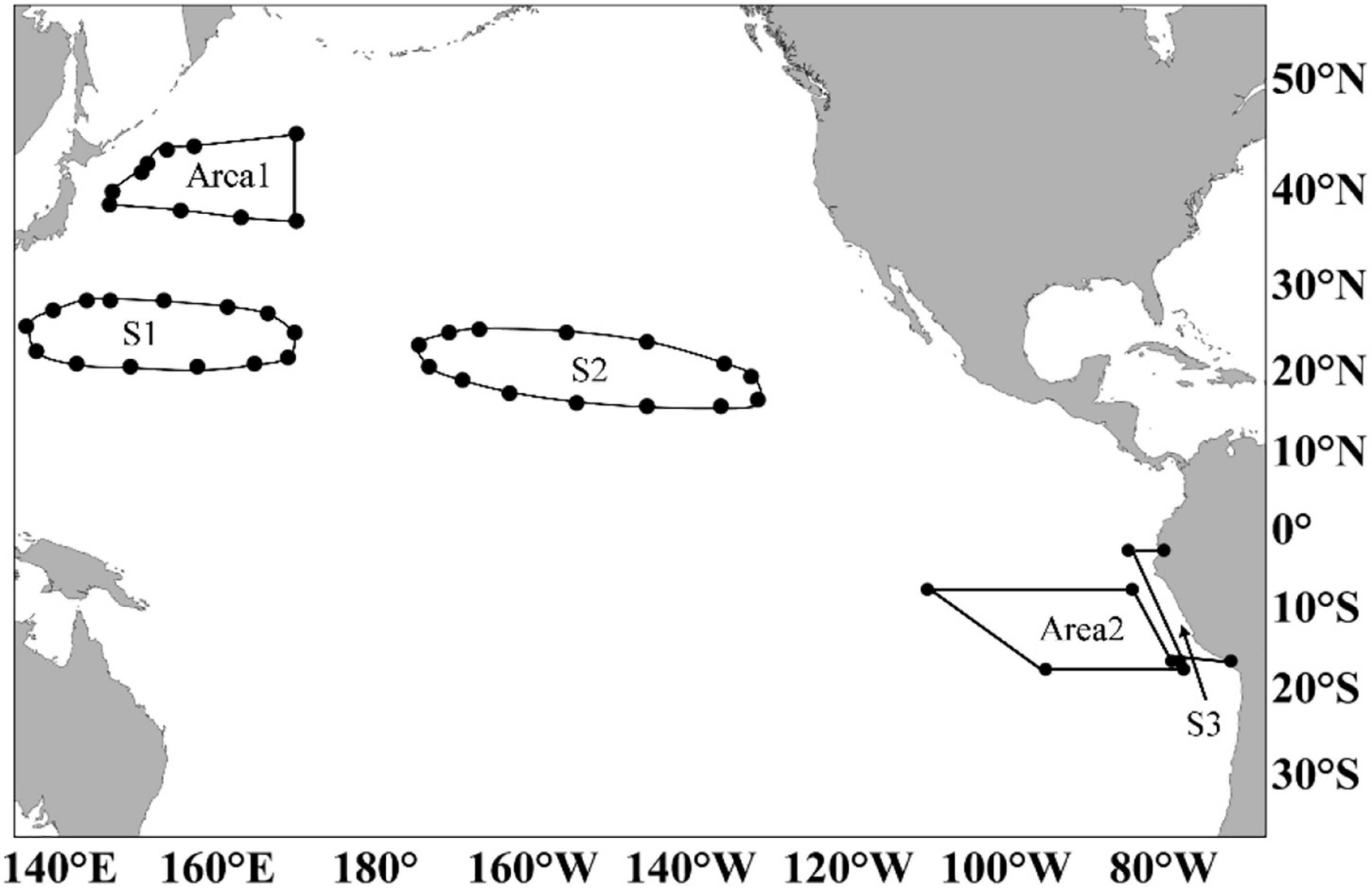
Figure 1. Spawning and feeding grounds (also fishing grounds) of Ommastrephes bartramii (stock of the winter-spring cohort) and Dosidicus gigas (off Peru Exclusive Economic Zone, PEEZ). S1 and S2: the spawning ground of O. bartramii; Area 1: the feeding ground (also the main fishing ground) of O. bartramii; S3: the spawning ground of D. gigas; Area 2: the feeding ground (also the main fishing ground) of D. gigas. Latitude and longitude points for drawing the boundary of S1, S2, S3, Area 1, and Area 2 are presented in Supplementary Table 1.

FIGURE 2

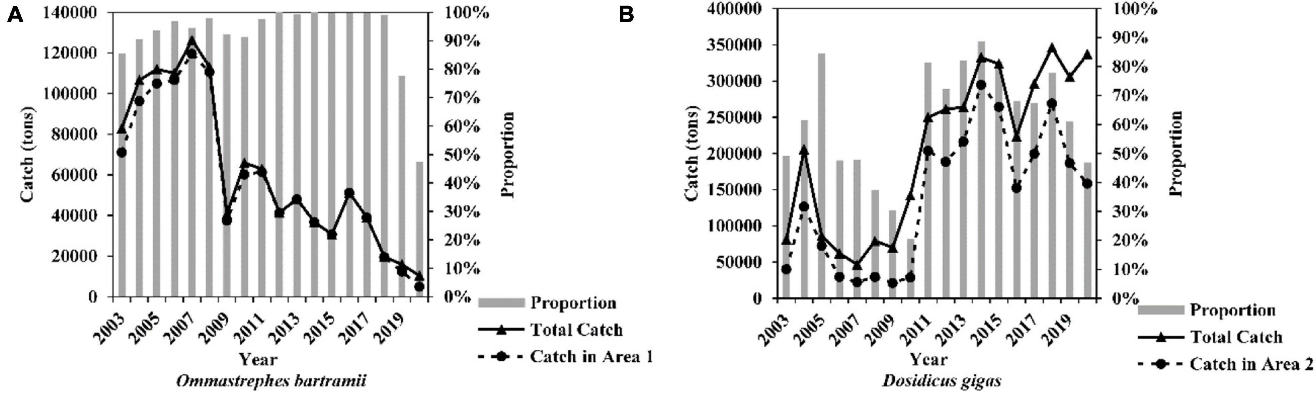
Figure 2. Annual catch, the catch, and its proportion within Area 1 (for Ommastrephes bartramii, A) and Area 2 (for Dosidicus gigas, B) in 2003–2020 for China squid-jigging fleets (Area 1: the Chinese main fishing ground of O. bartramii, west water of 170^°E. Area 2: the Chinese main fishing ground of D. gigas off Peru Exclusive Economic Zone waters (see Figure 1).

Before 2012, the main fishing grounds of D. gigas included the waters off PEEZ, off the Exclusive Economic Zone of Costa Rica or Chile (Chen et al., 2008; Liu et al., 2013a). After 2012, some squid-jigging fleets transferred to the equatorial waters (EW, 5°N-5°S, 95°-120°W), which has become a new fishing ground for D. gigas. Catch proportions in different regions exhibited high fluctuations in the 2000s due to the exploration of the new fishing grounds. Nevertheless, from 2011 to 2019, catch in the waters off PEEZ (Area 2, Figure 1, the boundary is based on the historical fishing location for D. gigas. The latitude and longitude points for drawing the boundary of Area 2 are listed in Supplementary Table 1), accounted for 61.02–88.60% of the overall catch (Figure 2B). D. gigas in different geographic regions have various size structures, age compositions (Liu et al., 2013a,2015b; Gong et al., 2017), and migration patterns (Liu et al., 2015a). Considering the complicated population classification, spawning ground locations, migration routes, and the fishery history of D. gigas, we only chose the fishery data of D. gigas within Area 2 for analysis in this study.

Cooper (2006) proposed that quantifying the fishery stock abundance could be determined from both the fishery-dependent data and the fishery-independent survey. Catch, effort or CPUE data derived from the fishery-dependent data, such as landing records, logbooks, vessel monitoring systems, and onboard observers, are commonly regarded as a crucial signal of fishery stock abundance dynamics (Cooper, 2006; Tian et al., 2009b; Pauly et al., 2013). A fishery-independent survey utilizing standardized sampling gears, including trawls, seines, hydroacoustics, and video, is expensive, particularly for the high sea fishery stocks (Cooper, 2006; Dennis et al., 2015). For example, for O. bartramii, only Japanese scientists conducted the driftnet surveys for the stock of the eastern autumn cohort before 2021 (Ichii et al., 2011; Igarashi et al., 2017). Currently, most studies of environment- and climate-induced oceanic squid stock abundance dynamics based on historical Chinese Squid-jigging fleets operation data consider the nominal CPUE as the squid abundance index (for example, Chen et al., 2007; Cao et al., 2009; Yu et al., 2017a,2021a,2021b). We followed their choice. And the nominal CPUE was defined as:

$\text{CPUE}=\mathrm{Catch}/\mathrm{Effort}$

where CPUE denotes the yearly nominal CPUE (ton/days) at Area 1 or Area 2; Catch represents the total yearly catch for all squid-jigging fleets at Area 1 or Area 2; Effort indicates total yearly fishing days at Area 1 or Area 2. The nominal CPUE could be regarded as a credible index of squid abundance for three reasons: (1) According to the collected squid-jigging fleets’ parameters and historical reports (Wang and Chen, 2005), Chinese squid-jigging fleets for O. bartramii and D. gigas had almost similar fishing powers, lamps, and engines; all fleets operated one time in a night during fishing season. (2) Study areas were restricted at the main fishing grounds for these two squids (Area 1 and Area 2) and without bycatch and (3) previous studies have done the CPUE standardization works to investigate if the catchability is constant for the O. bartramii and D. gigas abundance based on the same fishery data source in our analysis and suggested that the standardized CPUE and nominal CPUE were similar and had the same trends (Tian et al., 2009a; Xu et al., 2017). Thus, although catchability can be impacted by fishers’ behaviors, fishing gear type, ocean environment, management and other factors (Campbell, 2004), it is reasonable to infer that that the nominal CPUE is proportional to the squid abundance in this study.

Such as Seawater Temperature and Climate Index Data

Monthly SST data in the Pacific Ocean from 2002 to 2020 were available at the Oceanwatch database from NOAA.¹ The data were provided by the NOAA Coral Reef Watch (CRW) program with 5 km × 5 km spatial resolution.

ONI and PDOI were applied as the representatives for the climate events El Niño and La Niña and PDO. The ONI indicated the 3-month running mean of SST anomalies (NOAA ERSST.V5) in the Niño 3.4 region (5°N∼5°S, 120°∼170°W). The PDOI is the first principal component of monthly SST anomalies in the North Pacific Ocean (poleward of 20°N) based on the empirical orthogonal function. These data covered the period 2002–2020 and had the time resolution of a month, available in the NOAA Physical Sciences Laboratory.² Since the study aims to explore the abundance fluctuations of squids at annual and interannual scales, monthly ONI and PDOI were calculated as annual mean in the analysis (Supplementary Figure 1).

Analysis

Habitat Temperature Variabilities

Monthly SST at the two crucial habitats of O. bartramii and D. gigas, spawning ground, and feeding ground were employed to define habitat temperature variabilities. The location of these two squids’ spawning and feeding ground and the monthly periods of SST to be examined were based on their biological and fishery information described as follows.

(1) Ommastrephes bartramii (O. bartramii)

According to the analysis of squid hard tissues (beak, statolith), O. bartramii samples caught by China squid-jigging fleets hatched during October–June and peaked in January–April (Fang et al., 2016b). The result is consistent with previous studies of the spawning period for the stock of the winter-spring cohort (Nagasawa et al., 1998; Yatsu et al., 1998). Beak elemental concentration and larval surveys demonstrated that the stock of winter-spring cohort of O. bartramii possessed two spawning grounds located at the waters between 20°–30°N and 130°–170°E (S1) and between 20°–30°N and 130°–170°W (S2, Figure 1, the latitude and longitude points for drawing the boundary of S1 and S2 are provided in Supplementary Table 1; Ichii et al., 2004; Fang et al., 2019; Aho et al., 2021). Therefore, mean SST at S1 and S2 from January to April was adopted to describe the spawning ground temperature characteristics for O. bartramii.

From the spawning ground, the stock of winter-spring cohort of O. bartramii has northern migration to the feeding ground for growth (Bower and Ichii, 2005). The feeding ground of the stock of the winter-spring cohort of O. bartramii is distributed in the waters of 145°E-130°W, 35°N-50°N, and affected by the subarctic frontal zone (Bower and Ichii, 2005; Ichii et al., 2009; Aho et al., 2021). The feeding ground is distributed farther where the main fishing ground of China for O. bartramii in the North Pacific Ocean is located (Area 1, Figure 1). The historical catch records indicated that fishing operations at Area 1 last from June to November every year. This period is identical to the feeding time for the stock of winter—spring of O. bartramii (Fang et al., 2016b). Thus, mean SST at Area 1 from June to November was adopted to depict the feeding ground temperature characteristics of O. bartramii.

(2) Dosidicus gigas (D. gigas)

Statolith within 2008∼2010 and beak in 2013 of D. gigas samples caught by China squid-jigging fleets in the fishing ground suggested that the D. gigas off PEEZ waters hatched year-round but peaked from December of last year to May (Liu et al., 2013b; Hu et al., 2016). The spawning ground of D. gigas is believed to be along the continental slope of Peru and its internal shelf waters (Tafur and Rabí, 1997; Nigmatullin et al., 2001; Tafur et al., 2001; Sakai et al., 2008; Liu et al., 2013b). Liu et al. (2013b) revealed that the waters around the 11°S off PEEZ were also the spawning ground of D. gigas since more than 50% of the females sampled from these areas were mature. However, further experiments for the gonad of the female samples captured in the following years demonstrated that the individuals did not have spawning activity off PEEZ (unpublished data). Thus, this study restricted the spawning ground of D. gigas at the continental shelf and slope waters within PEEZ in this study according to the PEEZ line (S3, Figure 1. The latitude and longitude points for drawing the boundary of S3 can be seen in Supplementary Table 1). Consequently, mean SST at S3 from December of last year to May was selected to describe the spawning ground temperature characteristics for D. gigas.

Although D. gigas is a migratory species, unlike O. bartramii, there are no studies providing a specific distribution of its feeding grounds. D. gigas is an opportunistic predator with a wide range of food sources (Lorrain et al., 2011; Field et al., 2013; Liu et al., 2013a). Its short-scale migration patterns can be determined according to food conditions (Bazzino et al., 2010). As indicated in the diet analysis of the stomachs, more than 85% of individuals captured in the fishing ground had food remains (Liu et al., 2013a), reflecting that most species had feeding behaviors before being captured. Thus, the distribution of D. gigas fishing ground (Area 2) was applied to illustrate the range of its feeding ground in our study. The feeding ground ranges we used are analogs with the past report of the D. gigas’ geographic distribution off PEEZ waters by Nigmatullin et al. (2001). Considering that D. gigas could be captured through a year, mean SST at Area 2 from January to December was employed to represent its feeding ground temperature characteristics.

The habitat temperature variabilities are defined as the effective principal components of the SST at the squids’ two essential habitats (spawning and feeding ground) through life histories based on the PCA (Venables and Ripley, 2002). The PCA was used because too many factors were considered in the analysis according to the monthly mean SST dataset of O. bartramii and D. gigas. PCA can reduce the number of the factors and some independent principal components (PC_i, i = 1, 2, 3……) were extracted, accounting for a large proportion of the major characteristics for the habitat temperature. The analysis was based on the correlation matrix of the monthly mean SST dataset of O. bartramii and D. gigas. Furthermore, the number of PC_i was determined using the scree plot test method (Chatfield and Collins, 2018).

Hodrick—Prescott Filter Analysis

The annual and interannual abundance trends of O. bartramii and D. gigas and their PC_i were quantified by the Hodrick—Prescott filter analysis. Given a time series (TS), the method can be considered an additive decomposition: TS = ts + cs, where ts and cs denote the trend series and the cyclical series, respectively. It is a data-smoothing technique by minimizing an objective function that penalizes the sum of squares for cs with the sum of squares of second-order differences for ts in a time series (Hodrick and Prescott, 1997; Adiabouah, 2020). The objective function can be written as (Hodrick and Prescott, 1997):

$F=\sum _{t=1}^T{(t{s}_t-c{s}_t)}^2\sum _{t=2}^{T-1}{\left[\left(c{s}_{t+1}-c{s}_t\right)-\left(c{s}_t-c{s}_{t-1}\right)\right]}^2$

where T represents the time size, and λ refers to the smooth parameter and is set to 6. Through this method, it can be assumed that the annual fluctuations are short-term variations that belong to the cs and can be removed. Thus, the long-term trend (ts) defined as an interannual trend can be better observed.

Generalized Additive Model

We hypothesized that impacts of habitat temperature variabilities separately correspond to abundance fluctuations at different time scales (annual and interannual, respectively). And considering that the associations might consist of the non-linear effects, the GAM (Zhao et al., 2014; Wood, 2017) was used to detect the relationships between the ts of abundance (TA) and its PC_i (TPC_i) and between the cs of abundance (CA) and its PC_i (CPC_i) so as to validate this assumption. The model can be written as follows (Zhao et al., 2014):

$\text{TA}=\mathrm{\alpha }+{\displaystyle \sum _{\text{i}=1}^{\text{n}}}\mathrm{s}({\text{TPC}}_{\text{i}},\mathrm{k})+\mathrm{\epsilon }$

$\text{CA}=\mathrm{\alpha }+{\displaystyle \sum _{\text{i}=1}^{\text{n}}}\mathrm{s}({\text{CPC}}_{\text{i}},\mathrm{k})+\mathrm{\epsilon }$

where n denotes the number of PC_i we determined; α refers to the model intercept; s () indicates the smoothing function of TPC_i and CPC_i in which k represents the effective degrees of freedom determining the degree of non-linearity. k was restricted to a maximum of 3 to avoid over-fitting. ε suggests the random error with the normal distribution N (0, σ²). The Restricted Maximum Likelihood Estimation (RMLE) method was applied to fit the model. Moreover, the double penalty approach was used for model fitting (Marra and Wood, 2011), in which a second penalty on each smoothing function was added and only affected the functions in the null space, that is, one smoothing function might be flat (means no effect).

Choice of the Key TPC_i or CPC_i and Its Relationship With Climate Variability

Regarding model validation and choice of the key TPC_i or CPC_i that influence the abundance fluctuations, a cross-validation test would be conducted (the 18-year data were divided into two parts: training data for 16 years and validation data for 2 years). Training data were selected to build the model. Then, the model was used to predict the validation data. Whenever possible 16 training and 2 validation data set combinations within 2003∼2020 were used at the cross-validation test. Therefore, 153 sub-models were established. After the construction of all sub-models, model validation was evaluated by the performance of the predictability to the actual TA or CA and its changing trends. Specifically, statistical measures and regression analysis were applied in the model validation step.

(1) Statistical measures

The predictability to the actual TA or CA was verified by the mean absolute error (MAE) and root mean squared error (RMSE) between the validating and actual TA or CA. The predictability to the changing trend of TA or CA was validated by the mean absolute percentage change error (MAPCE) and root mean squared percentage change error (RMSPCE) according to the actual TA or CA values in the last year. The MAPCE and RMSPCE can be written as:

$\text{MAPCE}={\displaystyle \frac{1}{306}}{\displaystyle \sum \left|({\mathrm{X}}_{\mathrm{m},\mathrm{i}}-{\mathrm{X}}_{\mathrm{i}-1})-({\mathrm{X}}_{\text{i}}-{\mathrm{X}}_{\mathrm{i}-1})\right|\times 100\%}$

$\text{RMSPCE}=\sqrt{{\displaystyle \frac{1}{306}}{\displaystyle \sum {\left[({\mathrm{X}}_{\mathrm{m},\mathrm{i}}-{\mathrm{X}}_{\mathrm{i}-1})-({\mathrm{X}}_{\text{i}}-{\mathrm{X}}_{\mathrm{i}-1})\right]}^2\times 100\%}}$

where X_m,i and X_i denote the model predicted and actual TA or CA in year i, respectively, and X_i–1 represents the actual TA or CA in the last year i-1. Particularly, if i = 2003, the TA or CA in 2003 and 2004 (X_m,i–X_i–1 = X_m,2003–X₂₀₀₄ and X_i–X_i–1 = X₂₀₀₃–X₂₀₀₄) was used to calculate the MAPCE and RMSPCE.

(2) Regression analysis

Regression analysis is a common approach to evaluate the model goodness of fit. In the analysis, a simple regression model is used as follows:

$A=\mathrm{\alpha }(M)+\mathrm{\beta }$

where A and M denote the actual and model-predicted TA, CA, and their percentage change; α and β are the regression parameters indicating their slope and intercept; if α and β are not significantly different from 1 and 0, this implies that the model has an unbiased predictive skill (Chang et al., 2010; Zhao et al., 2014; Li et al., 2017).

After the model validation, key TPC_i and CPC_i were determined by the proportion of one TPC_i or CPC_i identified as significant (significant level: 0.05) in the sub-models for the 153 runs.

Key TPC_i or CPC_i was investigated by its corrections with ONI and PDOI. Previous studies demonstrated that El Niño and La Niña and PDO could affect the habitat and abundance fluctuation of O. bartramii and D. gigas in 0∼1-year effect (Chen et al., 2007; Yu et al., 2021a,b). Therefore, ONI, PDOI, and the values in 1-year lag (ONI_–1 and PDOI_–1) were included in the analysis. The best linear combination of climate indices (ONI, ONI_–1 PDOI, and PDOI_–1) was identified based on the step regression method with the minimum Akaike information criterion (AIC) to explain the variations of key TPC_i or CPC_i (Venables and Ripley, 2002).

All analyses in this study were implemented by the statistical software “R,” version 4.1.0 with package “mgcv” (version 1.8-35, Wood, 2017) and “mFilter” (version.1-5, Balcilar, 2019). The important abbreviations and their meaning for the statement of Results and Discussion are provided in Table A1.

Results

Abundance Fluctuation of O. bartramii and D. gigas

The overall abundance, TA, and CA of O. bartramii are illustrated in Figure 3A. Within 2003∼2020, the overall abundance of O. bartramii changed in 1.25∼4.11 t/day. Its TA indicated that the abundance of O. bartramii had a downward interannual trend from 2003 to 2013 and tended to increase after 2014. Its CA suggested that its abundance at an annual scale had about 3∼4-year cycles (defined as a period during relative lowest or highest value) such as 2012–2014 (3 years), 2006–2009 (4 years). The amplitude (differences between the lowest and highest value in one cycle) for each cycle was not similar. For example, the CA changed in –0.032∼0.1 t/day during the cycle of 2003∼2005, but in –0.89∼1.24 t/day within the next cycle (2006∼2009).

FIGURE 3

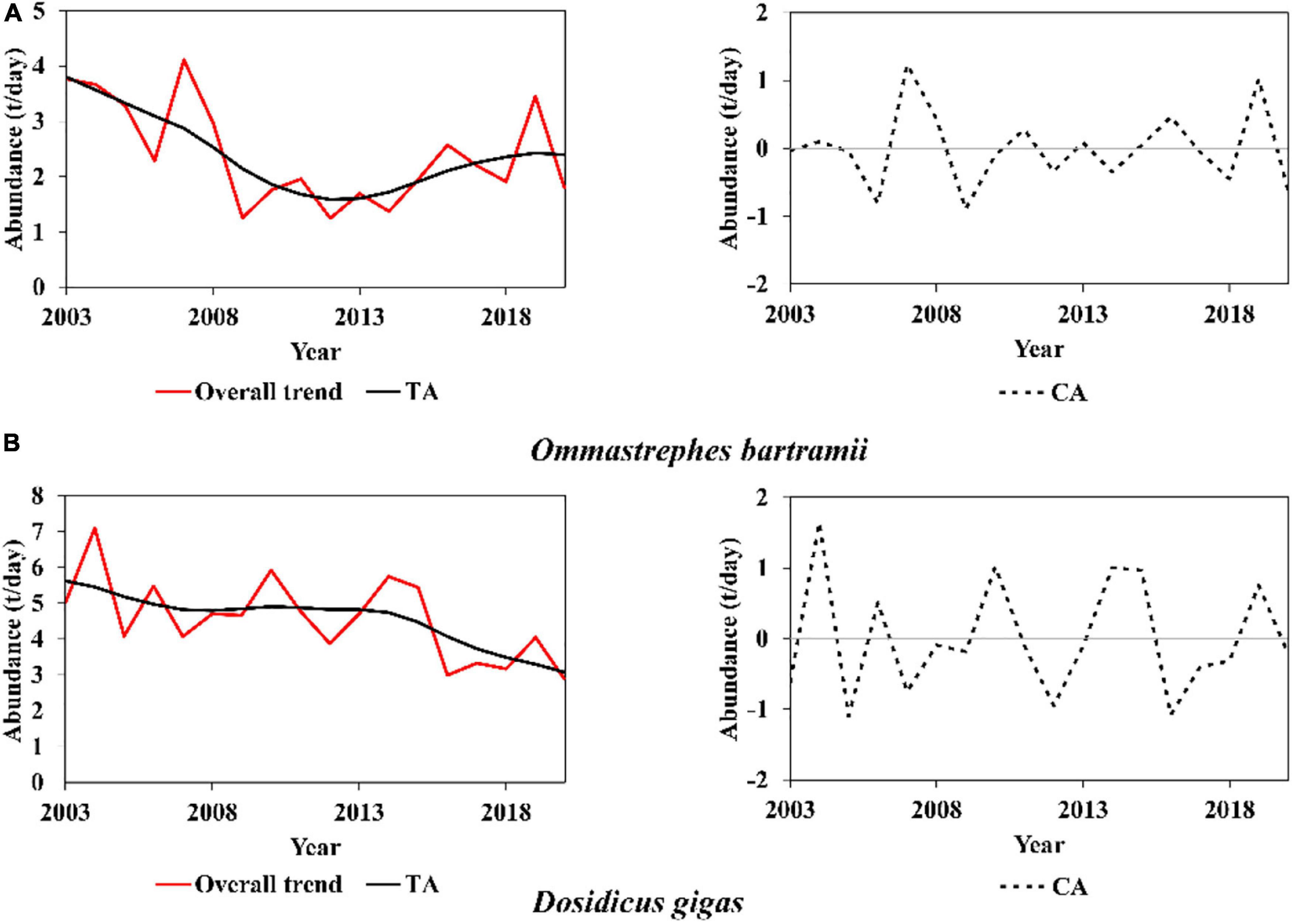
Figure 3. Overall, annual and interannual trends (annual: Cyclical series of abundance, CA, interannual: trend series of abundance, TA) based on Hodrick—Prescott filter analysis for (A) Ommastrephes bartramii and (B) Dosidicus gigas.

Within 2003∼2020, the overall abundance of D. gigas changed in 2.99∼7.10 t/day (Figure 3B). TA reflected that its interannual abundance trend kept decreasing from 2003 to 2018. But it remained steady during 2007∼2014 and started to decrease clearly after 2014. Moreover, the CA of D. gigas had a 3-year cycle within 2003∼2007 and a 5∼year cycle within 2007∼2020. Similar to O. bartramii, the amplitude of D. gigas for the 3∼year cycle was not similar. Nonetheless, the amplitude was similar (±1t/day) within the 5∼year cycle (2007∼2020).

Briefly, results showed different but not synchronous trends of abundance for O. bartramii and D. gigas. Concerning O. bartramii, the interannual abundance first decreased (2003∼2013) and then increased (after 2014). Regarding D. gigas, the interannual abundance kept decreasing within 2003∼2020. Their annual trends presented large fluctuations, with the changing amplitude greater than the increase or decrease speed of the interannual trend. There were no clear synchronous variations for the overall abundance, TA, and CA between O. bartramii and D. gigas (The correlation coefficients for the overall abundance, TA, and CA were 0.09, 0.33, and –0.07, respectively).

PCs Determined and Their Annual and Interannual Trend

The scree plot of eigenvalue and cumulative variance proportion of the SST at the spawning and feeding ground for O. bartramii indicated that six PC_i could be retained (Figure 4A). The first six PC_i totally explained 94.68% of the total variation. The results of D. gigas suggested that the first five PC_i need to be retained, accounting for 92.30% of the total variation (Figure 4B). Details of the PCA results, such as the retained loadings to each PC_i, are presented in Supplementary Tables 2, 3.

FIGURE 4

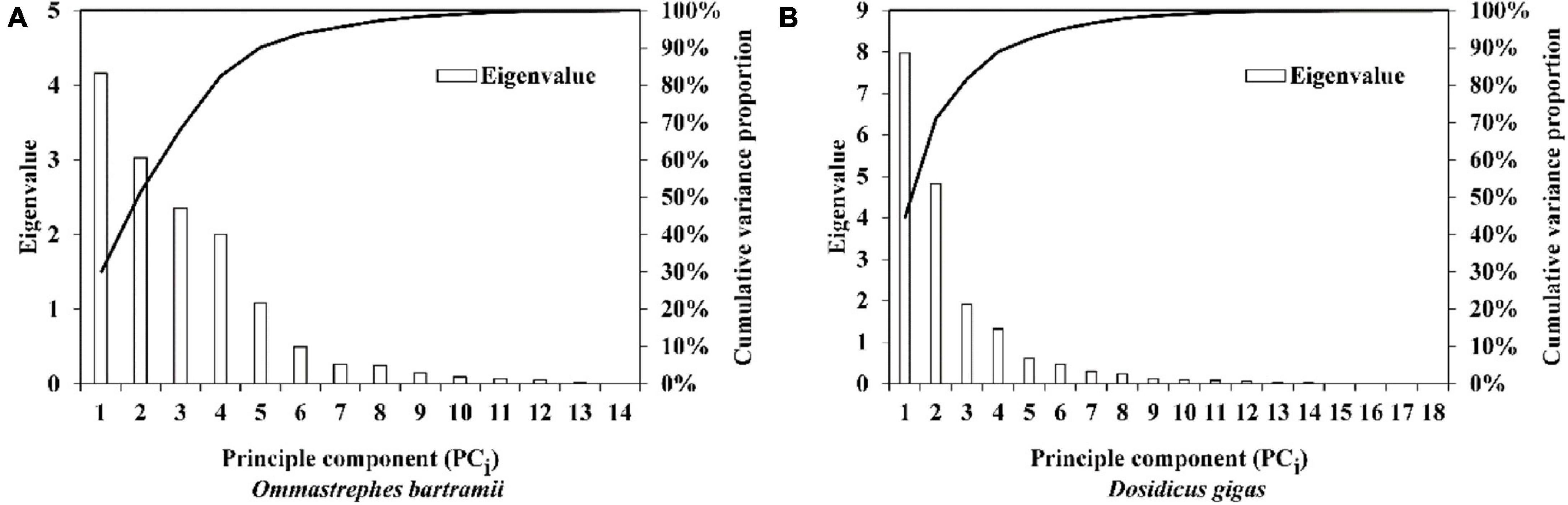
Figure 4. A scree plot from principal components analysis for the monthly sea surface temperature (SST) dataset at the spawning and feeding ground of (A) Ommastrephes bartramii and (B) Dosidicus gigas.

Figure 5 exhibits the overall, annual, and interannual trends of the first six PC_i (TPC_i and CPC_i) for O. bartramii from the Hodrick—Prescott filter analysis. Each TPC_i had its independent characteristics within 2003∼2020. TPC₁ possessed one and a half cycles with its increase within 2003∼2009 and 2016∼2020 and decrease within 2010∼2016 (Figure 5A). TPC₂ first decreased and then increased after 2012 (Figure 5B). TPC₃, TPC₄, and TPC₅ first increased, decreased, and increased, and then decreased within 2003∼2020, respectively (Figures 5C,E). TPC₆ changed little compared with the amplitude of other TPC_i (Figure 5F). There was no particular pattern of change for each CPC_i. Cycles appeared irregularly and could continue about 3∼5 years such as 2007∼2019 for CPC₂ (a cycle in 3 years, Figure 5B) and 2007∼2012 for CPC₄ (a cycle in 5 years, Figure 5D). Moreover, the amplitude in different cycles was not common. For example, a cycle of CPC₂ changed from –1.72 to 2.38 within 2015∼2018, while the range narrowed to –0.32∼0.43 for the cycle within 2018∼2020 (Figure 5B).

FIGURE 5

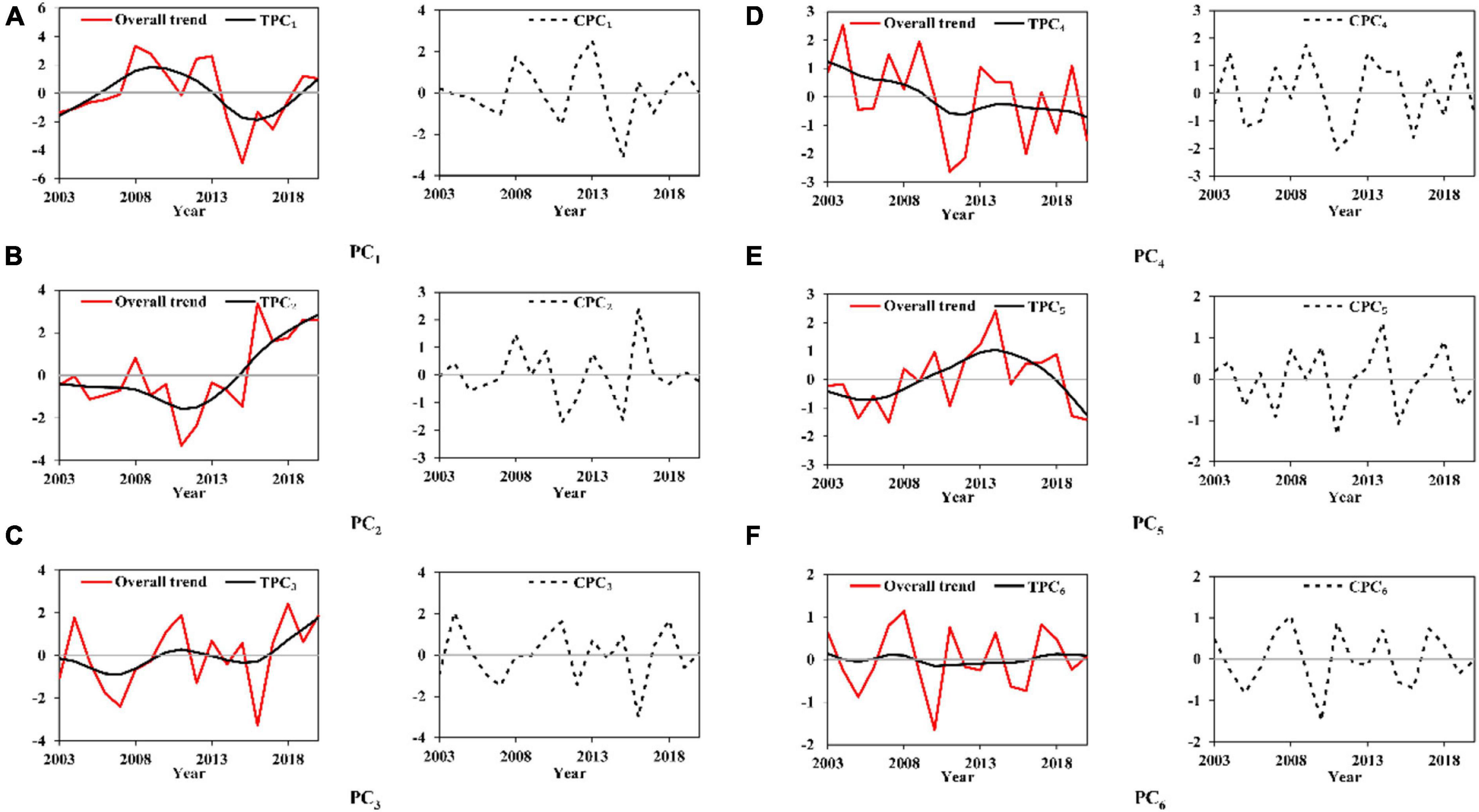
Figure 5. Overall, annual and interannual trends (CPC_i and TPC_i) of each principal component PC_i for the sea surface temperature at the spawning and feeding ground to Ommastrephes bartramii (Panels A–F indicate the Hodrick-Prescott filter analysis results of PC₁-PC₆).

Overall, annual and interannual trends of the first five PC_i for D. gigas are exhibited in Figure 6. Similar to the results of O. bartramii, each TPC_i had its trend with independent shape through time. TPC₁ had an entire cycle within 2011∼2020 while slightly decreasing before 2011 (Figure 6A). TPC₂ had a cycle of increasing in 2003∼2007 and decreasing after 2011 (Figure 6B). Within 2003∼2020, TPC₃, TPC₄, and TPC₅ generally increased, decreased, and slightly decreased, respectively (Figures 6C–E). There was no particular pattern of change for each CPC_i. Irregular cycles and different amplitudes could also be observed on the cycles for each CPC_i (Figure 6).

FIGURE 6

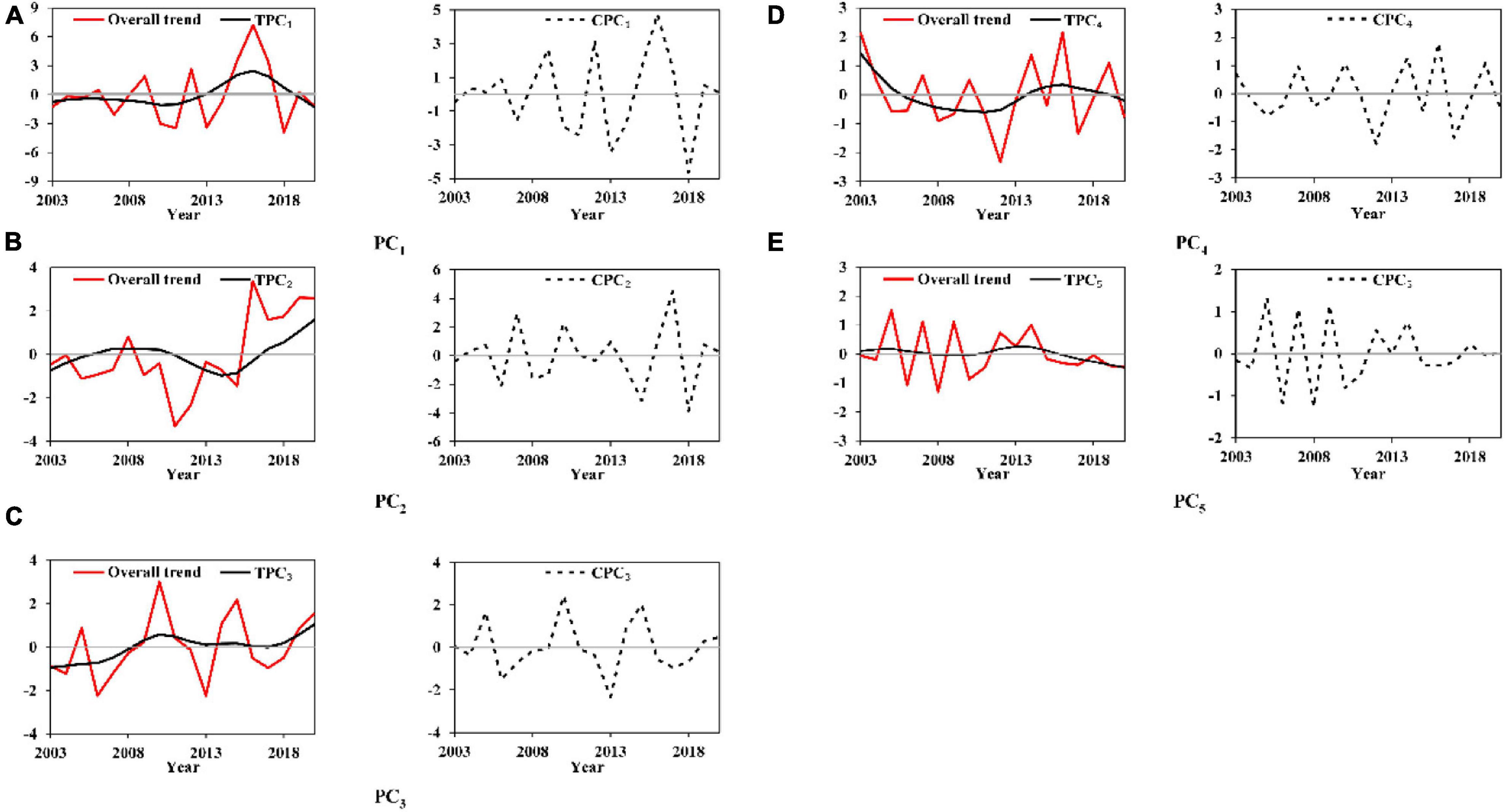
Figure 6. Overall, annual and interannual trends (CPC_i and TPC_i) of each principal component PC_i for the sea surface temperature at the spawning and feeding ground to Dosidicus gigas. (Panels A–E indicate the Hodrick-Prescott filter analysis results of PC₁-PC₅).

Briefly, each TPC_i and CPC_i for these two squids had its independent characteristics. CPC_i had larger fluctuations than those of TPC_i by the irregular cycles and different amplitudes along the years.

Generalized Additive Model Validation and Key TPC_i or CPC_i Choice

Sub-models of GAM for TA to O. bartramii and D. gigas could perform acceptable predictions for the validation data (Figures 7, 8). MAE and RMSE for O. bartramii were 0.031 t/day and 0.046 t/day, respectively. Regarding D. gigas, MAE and RMSE were 0.11t/day and 0.14 t/day, respectively. MAPCE and RMAPCE for the TA of O. bartramii were 1.39 and 2.04%, respectively. MAPCE and RMAPCE for the TA of D. gigas were 2.48 and 3.04%, respectively. The errors mainly occurred when TA_i-TA_i–1 was near 0% (–1∼3%, Figures 7C, 8C). On the contrary, sub-models of GAM for CA to O. bartramii and D. gigas presented poor predictions for the validation data (Figures 9, 10). MAE and RMSE for O. bartramii were 0.49 t/day and 0.67 t/day, respectively. For D. gigas, MAE and RMSE were 0.89 t/day and 1.05 t/day, respectively. MAPCE and RMAPCE for the CA of O. bartramii were 477.24 and 1054.93%, respectively, and 439.05 and 262.48% for the CA of D. gigas.

FIGURE 7

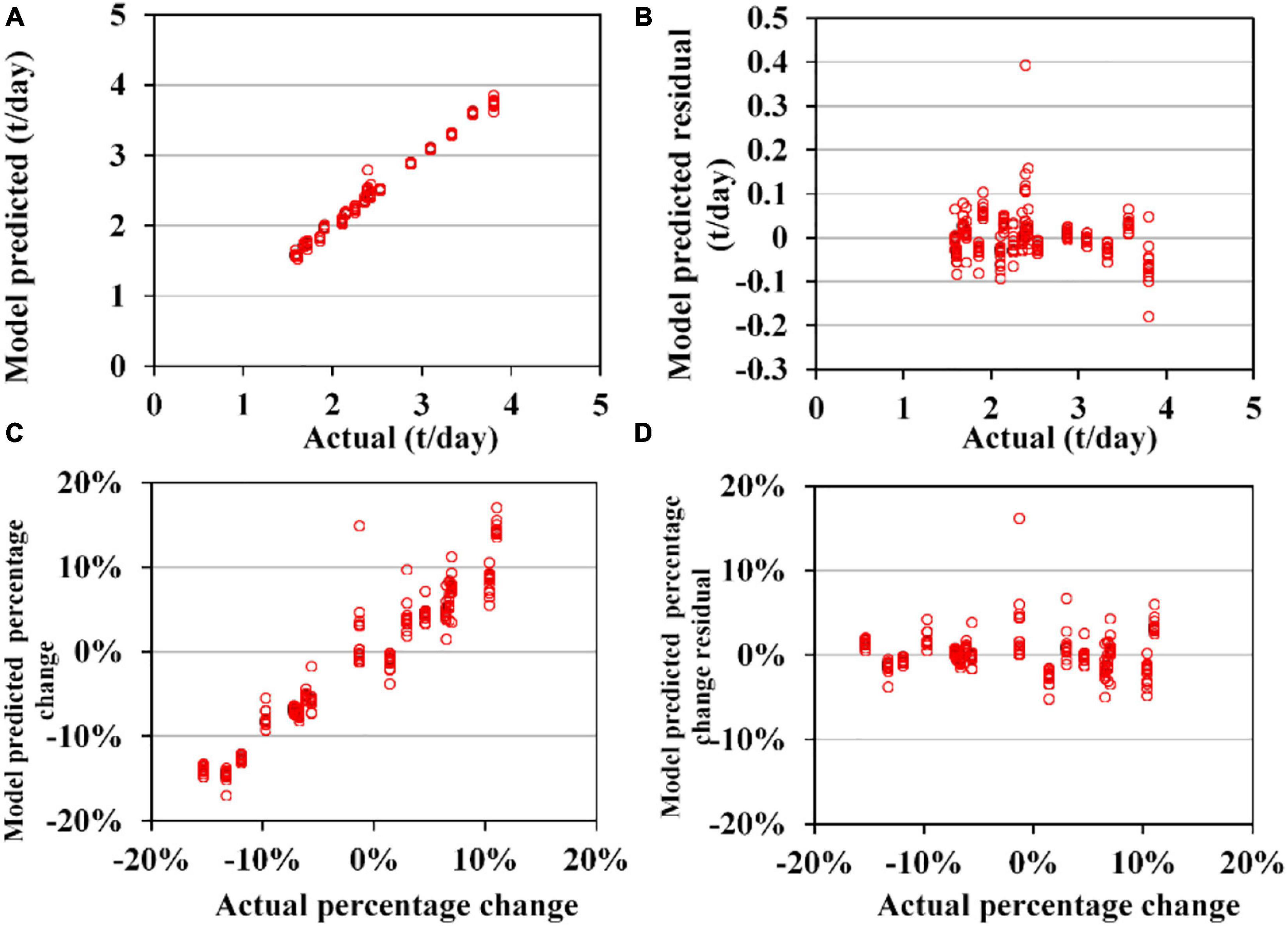
Figure 7. Cross-validation results of 153 sub-models of generalized additive models (GAM) for the interannual abundance trend of Ommastrephes bartramii (TA). (A) Model-predicted and actual TA; (B) model-predicted residual and actual TA; (C) model-predicted and actual TA percentage change compared with the last year (except for 2003 in which it is compared with the year 2004); (D) the model predicted the residual and actual value for TA percentage change compared with the last year.

FIGURE 8

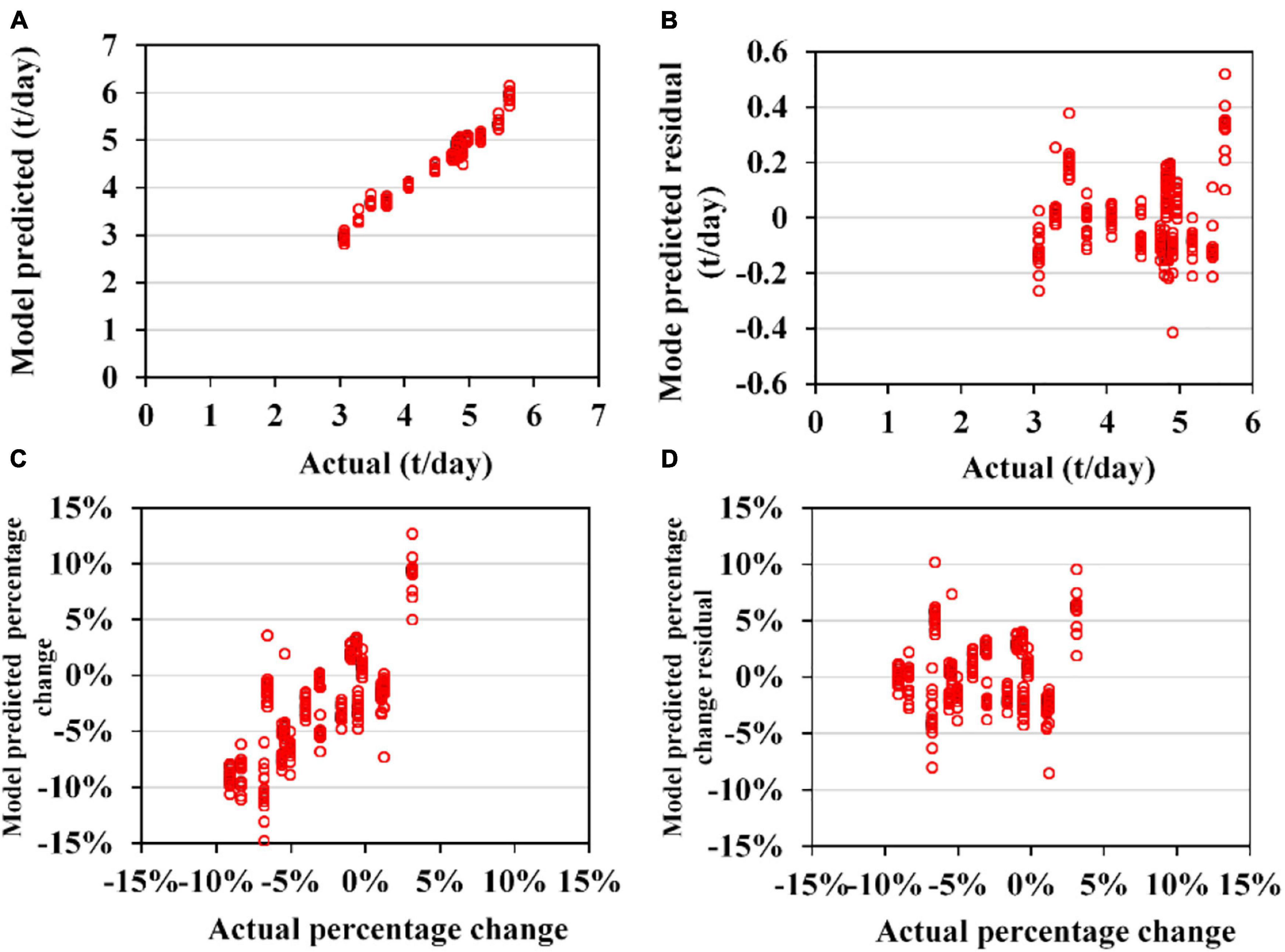
Figure 8. Cross-validation results of 153 sub-models of generalized additive models (GAM) for the interannual abundance trend of Dosidicus gigas (TA). (A) Model-predicted and actual TA; (B) model-predicted residual and actual TA; (C) model-predicted and actual TA percentage change compared with the last year (except for 2003 in which it is compared with the year 2004); (D) the model predicted the residual and actual value for TA percentage change compared with the last year.

FIGURE 9

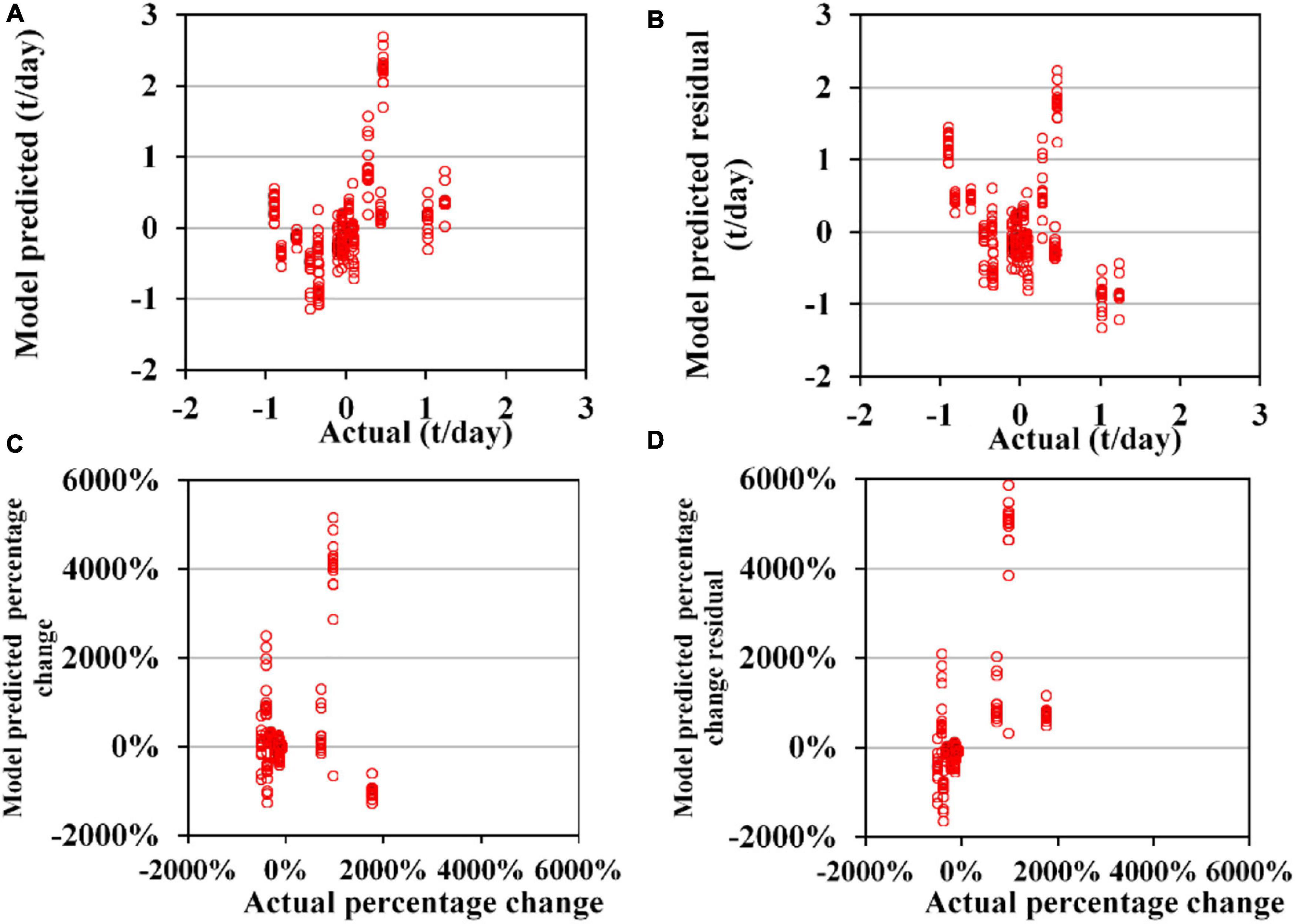
Figure 9. Cross-validation results of 153 sub-models of generalized additive models (GAM) for the annual trend of the abundance of Ommastrephes bartramii (CA). (A) Model-predicted residual and actual CA; (B) residual between model-predicted and actual CA; (C) model-predicted and actual CA percentage change compared with the last year (except for 2003 in which it is compared with the year 2004); (D) the model predicted the residual and actual value for CA percentage change compared with the last year.

FIGURE 10

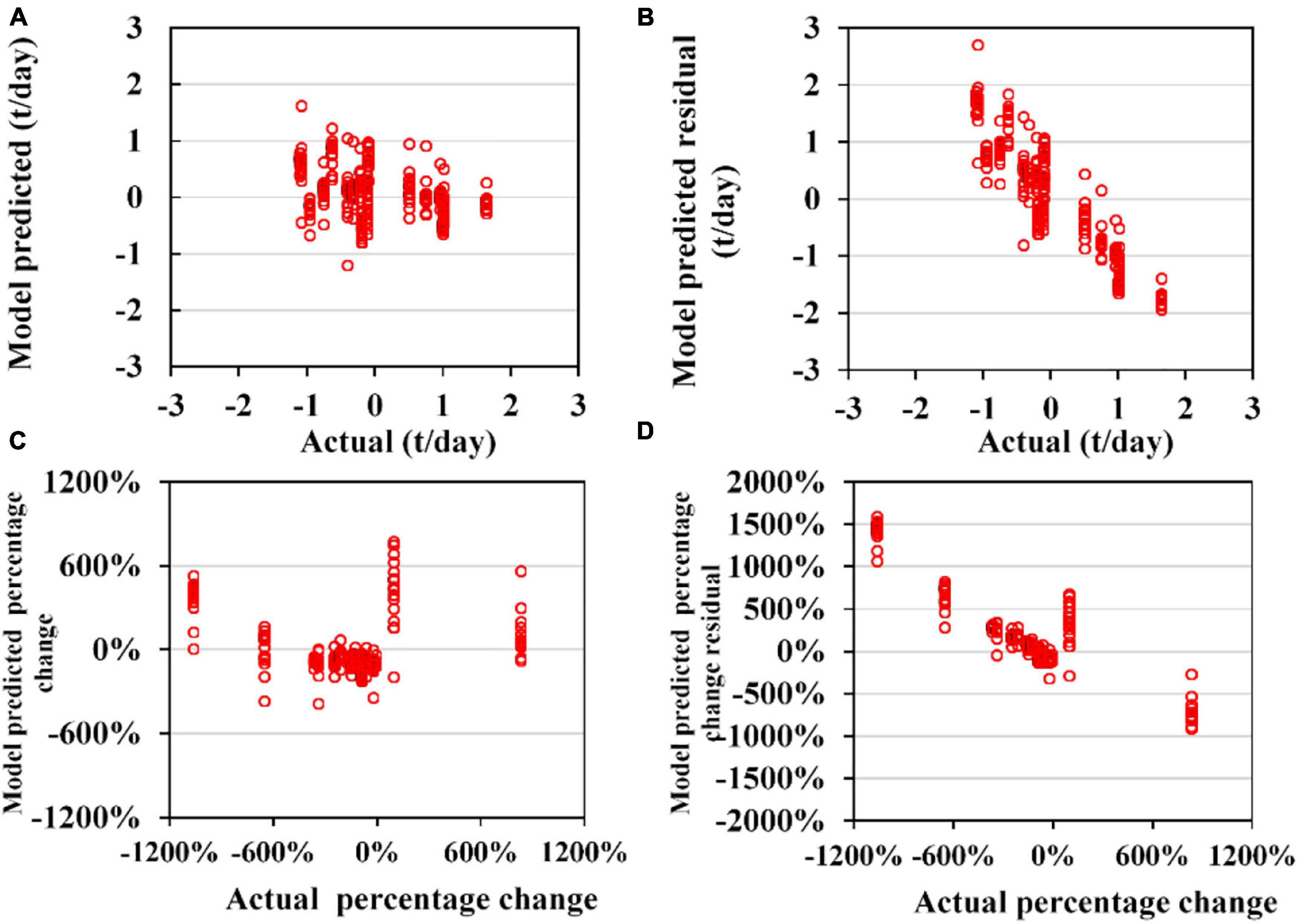
Figure 10. Cross-validation results of 153 sub-models of generalized additive models (GAM) for the annual trend of the abundance of D. gigas (CA). (A) Model-predicted and actual CA; (B) model-predicted residual and actual CA; (C) model-predicted and actual CA percentage change compared with the last year (except for 2003 in which it is compared with the year 2004); (D) the model predicted the residual and actual value for CA percentage change compared with the last year.

Regression analysis (Table 1) showed the model-predicted TA of O. bartramii positively changed with actual TA. The slope α was closer 1 (0.989), but α and intercept β were significantly different from 1 and 0 (p < 0.05). However, the coefficients α and β for the changes in the TA percentage did not present significant difference with 1 and 0 (p > 0.05). Regarding D. gigas, the model-predicted TA positively changed with the actual TA and the coefficients α and β were not significantly different from 1 and 0 (p > 0.05). But coefficients α and β for the TA percentage change had significant difference with 1 and 0 (p < 0.05). For the CA models, the null hypothesis (H₀: α = 1, β = 0) was believed to be rejected because P-values for the coefficients α and β were less than 0.05 (except for the β in the regression of the CA for O. bartramii).

TABLE 1

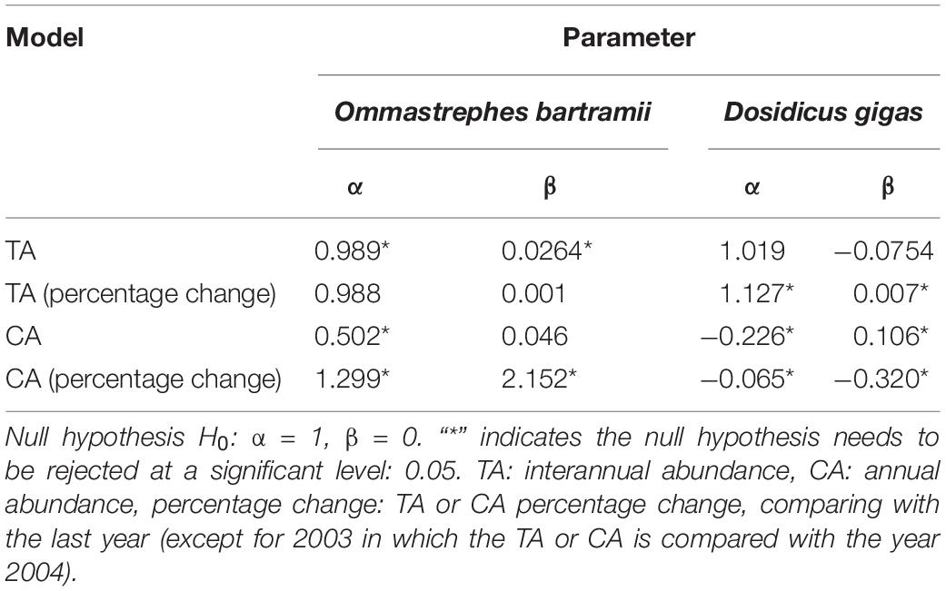
Table 1. Results of the regression models [A = α (M) + β] of actual and model-predicted values for the validation data in the cross-validation.

In summary, GAM performed well on the relationship between the abundance trend and its habitat temperature variabilities at the interannual scale while presenting poor results at the annual scale for both O. bartramii and D. gigas. In terms of the MAE, MSE, MAPCE, and RMAPCE values, GAM exhibited a better result for O. bartramii in the relationship of TA∼TPC_i than D. gigas. But from the results of regression analysis, GAM gave better predictions for the TA changing trend but had the slightly weaker predictive ability for the TA value of O. bartramii than D. gigas.

Given the poor results of CA∼CPC_i for both two squids, only key TPC_i would be determined. According to the proportion of each TPC_i identified as significant in the 153 sub-models of GAM (Table 2), TPC₁, TPC₄, and TPC₅ were considered the primary TPC_i affecting the abundance of O. bartramii with all the sub-model identifying them as significant (p < 0.05). TPC₃ was the second essential TPC_i with the proportion confirming as significant (p < 0.05) in sub-models at 92.81%. TPC₂ and TPC₆ were regarded as the least essential TPC_i with only 32.68% and 18.95% of sub-models identifying it as significant. For D. gigas, TPC₅ was taken as the most primary TPC_i with all the sub-models identifying it as significant (p < 0.05, Table 2), followed by TPC₁ (99.35%) and TPC₄ (85.62%). The least important TPC_i was TPC₂ and TPC₃ with the proportion as significance in sub-models as 54.90 and 29.41%, respectively. Therefore, TPC₁, TPC₃, TPC₄, and TPC₅ for O. bartramii and TPC₁, TPC₄, and TPC₅ for D. gigas were believed to be the key TPC_i affecting the interannual abundance trend of O. bartramii and D. gigas. Thus, they were used for further analysis.

TABLE 2

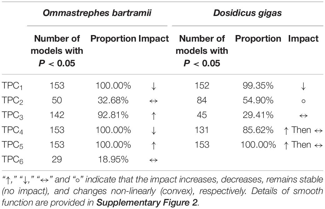
Table 2. The proportion of each trend series of principal component (TPC_i) identified as significant (significant level α: 0.05) in all sub-models (n = 153) of generalized additive models (GAM) for Ommastrephes bartramii and Dosidicus gigas, and the impact of each TPC_i on the TA (smooth function) based on the generalized additive models (GAM) with all-year data (2003∼2020).

Additionally, GAM was operated with all-year data (2003∼2020) to explore the impact of each TPC_i on TA (Supplementary Table 2). The impact of TPC₁, TPC₃, TPC₄, and TPC₅ on TA for O. bartramii decreased, increased, decreased, and increased, respectively. The impact of TPC₁, TPC₄, and TPC₅ on TA for D. gigas decreased, increased, stopped changing, and increased, respectively (Supplementary Table 2 and Supplementary Figure 2). Details of smooth function plots are provided in Supplementary Figure 2.

Key TPC_i and Its Association With Climate Index

According to step regression analysis with minimum AIC value (Table 3), TPC₁ for O. bartramii could be explained by PDOI. TPC₁ and PDOI had a negative relationship with the decrease that occurred when PDO changed from the warm phase to the cold phase, and vice versa (Figure 6A and Supplementary Figure 1). TPC₅ could be explained by PDOI and PDOI_–1. Nonetheless, the regression result was not convincing because no significant relationship was found from the ANOVA test (p > 0.05), lower R² (0.19), and no significant parameters. No combination of parameters was demonstrated to be better compared to the null model for TPC₃ and TPC₄ (TPC₃/TPC₄ ∼ Intercept). Regression results for D. gigas suggested that TPC₁ could be explained by PDOI. TPC₁ and PDOI had a positive relationship with the value generally along the trend of PDOI (Figure 6A and Supplementary Figure 1). TPC₅ could be explained by PDOI and PDOI_–1, although the regression was not significant (P = 0.07). Furthermore, TPC₄ was related to ONI and ONI_–1, and both the model and its parameters were significant (p < 0.05).

TABLE 3

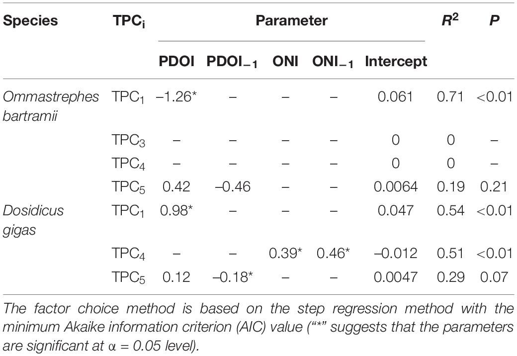
Table 3. Best results for the relationship between each significant trend series of principal component (TPC_i) and climate indices (Pacific Decadal Oscillation Index, PDOI, and Oceanic Niño Index, ONI. “–1” at the subscript of PDOI and ONI indicates its 1-year-lag effect).

Discussion

Generalized Additive Model Performance for the TA_i and CA_i

It was assumed in this study that the squids’ habitat temperature annual and interannual variability was separately related to the abundance fluctuation at the corresponding scale. The hypothesis was tested by the GAM model and cross-validation test. Results demonstrated that the model only performed well on modeling the TA (Figures 7–10). This indicated that the abundance fluctuations of O. bartramii and D. gigas could be investigated by their habitat temperature variabilities at the interannual scale instead of the annual scale. Potential mechanisms might be induced by the complicated relationship between ocean environment and oceanic squids’ unique life histories. The oceanic squids are short-lived species with a life span of 1 year for O. bartramii and 1∼2 years for D. gigas (O’Dor, 1998; Ichii et al., 2009; Arkhipkin et al., 2015b). During their short life histories, the abundance fluctuations are highly sensitive to the large- and small-scale environmental changes (Anderson and Rodhouse, 2001). The abundance-environment relationship below the annual scale has been widely investigated in previous studies. For example, Ichii et al. (2011) proposed the stock abundance of the autumn cohort of O. bartramii coincided with the Chl-a concentration in their spawning ground and feeding ground. At the feeding ground of the O. bartramii, Nishikawa et al. (2014) discovered that the higher CPUE usually occurred at the location with higher SST or lower SST anomaly. Yu et al. (2016c) observed that food availability on the spawning ground, SST, and Chl-a concentration on the fishing ground together influenced the stock abundance of the winter-spring cohort of O. bartramii. With respect to D. gigas, Waluda et al. (2006) and Waluda and Rodhouse (2006) reported that the D. gigas abundance off Peru waters was associated with the mesoscale SST variability controlled by El Niño and La Niña. In the Gulf of California, the concentration of D. gigas was controlled by SST and Chl-a (Robinson et al., 2013). Yu et al. (2019) indicated that the seasonal CPUE was affected by the SST, net primary production (NPP), and sea surface height anomaly (SSHA). In short, many results of previous studies confirmed that the intra- and annual abundance fluctuations of O. bartramii and D. gigas were sensitive to environmental changes, including, not only temperature, but also other factors such as physical oceanic environmental parameters (such as Chl-a, NPP, and SSHA). It might be the reason for a poor relationship found on CA∼CPC since we only used habitat temperature as the explanatory factor (Figures 9, 10).

On the contrary, the results suggested that the interannual abundance fluctuations of O. bartramii and D. gigas could be investigated by their habitat temperature variabilities. The CA is observed to have large fluctuations influenced by many environmental factors. In fact, for squid species with 1-year life span, these environmental factors and recruitment dynamics are only related to their abundance in the same year (in other words, abundance is not associated with its spawning biomass or the abundance in previous years, O’Dor, 1998; Ichii et al., 2009; Arkhipkin et al., 2015a). Yu et al. (2016c) verified that the oceanic squids could respond quickly to regional and large-scale environmental conditions. Therefore, TA may reflect only the effects of long-term environmental and climate variabilities on the squids’ abundance fluctuations when the short-term CA is removed.

Interestingly, why is the habitat temperature essential to the effects of long-term environmental and climate variabilities? The annual and interannual abundance fluctuations of these two squids had been widely reported by Yatsu et al. (2000), Igarashi et al. (2017), Alabia et al. (2020) and Yu et al. (2021a,b) for O. bartramii and Taipe et al. (2001) and Yu et al. (2021a,b) for D. gigas. All studies considered SST and revealed powerful relationships wherein the habitat temperature factor is the most imperative one in squids’ abundance dynamics. From the biological perspective, Sakai et al. (2004) discovered that higher temperatures within optimum ranges could improve squids’ recruitment by reducing the hatching time and benefiting embryonic development. The abundance of the stock of the winter-spring cohort of O. bartramii could be largely controlled by the proportion of favorable-SST areas at the spawning ground (Cao et al., 2009). Additionally, squid growth responds to temperature mostly in nature (Jackson and Domeier, 2003; Forsythe, 2004). Temperature is also essential for the maturity and reproduction of O. bartramii and D. gigas (Bower and Ichii, 2005; Liu et al., 2013a). In short, temperature can be the most important one affecting the entire life history of O. bartramii and D. gigas (Yatsu et al., 2000; Ichii et al., 2009; Yu et al., 2021a). From another perspective, SST, as commonly used data in the fishery oceanography, is also adopted to describe the meso-scale and large-scale oceanic processes, such as fronts (Redelsperger et al., 2019), eddys (Jia et al., 2019), El Niño and La Niña (Hayashi et al., 2020), PDO (Mantua et al., 1997), and ocean warming (Cheng et al., 2019). Thus, temperature and temperature-related oceanic processes related to their abundance might be consequently reflected on their interannual abundance fluctuations, considering the temperature plays a key role in squids’ life history.

As demonstrated by our cross-validation results, the TA and its changing trends of validation data could not be all predicted well (Table 1 and Figures 7C,D, 8C,D). Based on our fishery data, an additional hindcast for the TA of O. bartramii in 1995∼2002 was made by the GAM model for the data over 2003∼2020 (Supplementary Figure 3). The results indicated the overall shape of TA between the hindcast and actual value was similar; however, an error occurred on the TA-changing trend in 1998∼1999. Thus, a conclusion cannot be easily extended to the interannual scale that the temperature plays a critical role in the interannual abundance fluctuations, owing to some potential mechanisms. Previous studies also indicated that other factors (partly) independent from temperature were also important. For example, according to the commercial driftnet fishery monitoring data, Yatsu et al. (2000) observed the interannual stock abundance of the autumn cohort of O. bartramii and discovered relatively low-level abundance in 1978∼1992 and an increasing trend after 1992. They revealed that the interannual variability might be caused by fishing mortality and SST. Nishikawa et al. (2014, 2015), Igarashi et al. (2017), and Yu et al. (2016a) presented that the wind-induced Ekman transport and mixed layer depth could be associated with the abundance of O. bartramii. CPUE of the autumn cohort of O. bartramii was considered to be related to the location of the transition zone chlorophyll front (TZCF, Ichii et al., 2011). Medellín-Ortiz et al. (2016) demonstrated that the population size of D. gigas along Baja California’s west coast was significantly affected by the primary productivity, catches of Pacific sardine (Sardinops caeruleus), and North Pacific Gyre Oscillation (NPGO). To summarize, temperature can be connected with other oceanic processes, while these factors would not be completely included in the information of habitat temperature variabilities, resulting in the errors of the model predictive performance. Thus, other potential factors should be considered in the future to explore the differences in their importance. This can deepen our understanding of the interaction between the interannual abundance fluctuations and environmental variabilities for O. bartramii and D. gigas.

Abundance Fluctuations in Relation to Climate Variability

Our results have three findings related to PDO regarding these two squids. (1) Based on the GAM results (Supplementary Table 2 and Supplementary Figure 2), the impacts of TPC₁ to TA of both O. bartramii and D. gigas were similar (decrease); (2) TPC₁ of O. bartramii was negatively related to PDOI, while TPC₁ of D. gigas had a positive correlation with PDOI; (3) the PDO-related TPC₁ between O. bartramii and D. gigas had a significant negative relationship (r = –0.76, p < 0.01). Thus, the mechanism of the effect of PDO on the O. bartramii and D. gigas is that PDO could induce opposite conditions of habitat temperature variabilities for these two squid species while acting similarly to the interannual abundance fluctuations for O. bartramii and D. gigas through habitat temperature variabilities. This is consistent with the conclusions of Yu et al. (2021b) who investigated the habitat variations of O. bartramii and D. gigas in 1950∼2015 and their relationship with PDO. They revealed that, during the cold PDO phase, SST anomaly increased but led to a decrease for the area with suitable SST for O. bartramii, while the decrease of SST anomaly led to the formation of areas with more suitable SST for D. gigas, and vice versa. What is more, SST and other environmental factors were usually included in the habitat suitability index model (Yu et al., 2017b,2021b; Alabia et al., 2020). This model explained well in the association between the PDO and the spatial and temporal abundance variabilities for O. bartramii and D. gigas and, again, demonstrated PDO-induced opposite habitat conditions between these two squids.

In our studies, by the cross-validation test of GAM, TPC₁ of O. bartramii was believed to be the primary TPC_i affecting the interannual abundance trend. Regarding D. gigas, TPC₁ was the second important factor (Table 2). This TPC_i was related to PDO according to the step regression analysis (Table 3). Moreover, the PDO affects the abundance of O. bartramii and D. gigas through its habitat environment (including temperature), in line with the statement of previous studies, and TPC₁ of O. bartramii and D. gigas accounts for the most proportion of variance of habitat temperature variabilities in PCA. It can be concluded that the PDO is an essential climatic factor affecting the interannual abundance fluctuations of squids through habitat temperature variabilities.

A limitation of our studies is that ONI and PDOI were used in the annual mean, only to conduct the preliminary analysis between habitat temperature variabilities and climate variabilities. It can be confirmed in the PDO situations since the warm or cold phases last for many years. Nevertheless, the monthly ONI data indicated that the events of El Niño and La Niña last for 5∼19 months in 2003∼2020. As a result, we might be unable to well examine the impacts of El Niño and La Niña in the relationship between TPC_i and the annual mean of ONI. From the step regressions results, TPC₄ of D. gigas was also a crucial TPC_i and related to ONI and ONI_–1 (Tables 2, 3) while not all sub-models in the cross-validation test identified TPC₄ as significant (85.62%, Table 2). None of the key TPC_i of O. bartramii could be explained by ONI and ONI_–1 (Table 3). The effects of El Niño and La Niña on these two squids’ abundance have also been widely documented (Ichii et al., 2002; Waluda et al., 2006; Chen et al., 2007; Yu et al., 2021a). Moreover, the long-term abundance fluctuation of D. gigas associated with the environmental changes by El Niño was reported at the Gulf of California (Robinson et al., 2016; Frawley et al., 2019). After the El Niño events in 2009, the landings of D. gigas declined due to the warmer waters, weak winter/spring winds, and extremely low Chl-a along the Gulf of California in the following years. From our analysis, a similar trend in decrease can be found in TA of D. gigas after the 2015∼2016 El Niño events (Figure 3B) and TPC₄ declined (Figure 6D). From the GAM results, TA increased with TPC₄ (Supplementary Figure 2B). But the TA of D. gigas kept steady during 2007∼2014 and TPC₄ increased after the El Niño events in 2009 (Figures 3B, 6D). In previous studies, only a 2-month lag effect between the SST anomaly at Niño 3.4 and Niño 1 + 2 regions was observed, as well as the SST at these two squids’ fishing (feeding) ground, which consequently affected their abundance (Yu et al., 2021a). This indicates the stock/group of O. bartramii and D. gigas we studied responses quickly for the El Niño and La Niña when habitat temperature conditions changed. Therefore, it is not clear whether the effects of El Niño and La Niña on the abundance fluctuations of D. gigas we studied in the waters off PEEZ are just below the annual scale or can be extended to interannual scale. It is suggested that further research needs to collect the data with a wider year range to evaluate it.

Additionally, TPC₅ of O. bartramii and D. gigas was also an important TPC_i affecting the interannual abundance trend based on the cross-validation test of GAM. However, it was not related well to PDO and PDO_–1 (Table 3, P = 0.07). Moreover, there is another key TPC_i (TPC₃ and TPC₄ for O. bartramii, Table 2) that could not be explained by the PDOI and ONI we examined. One possible reason is that other environmental and climate variabilities drive the variations of key TPC_i. These factors, which are independent of the El Niño and La Niña and PDO effects but related to habitat temperature variabilities, indirectly affect the interannual fluctuations of squid abundance. In other studies of cephalopod’s fishery, for example, common Chinese cuttlefish catches were demonstrated to be negatively affected by both Asian Monsoon Index (AMI) and winter SST in the East China Sea (Pang et al., 2018). Meanwhile, the SST had an association with Asian Monsoon (Li et al., 2008; Bao and Ren, 2014). November Arctic Oscillation had been reported to impact the subsequent SST at tropical Pacific Ocean (Chen et al., 2015, 2018). There is evidence that the Arctic Oscillation-related sea ice drives the variations of tropical Pacific SST (Rigor et al., 2002; Purich et al., 2016). These emphasized again the importance of combining other potential factors in future works.

Finally, we conclude that the PDO and El Niño and La Niña can impact the abundance fluctuations in the same way but play an opposite role for the suitable habitat between the O. bartramii and D. gigas from the results of Yu et al. (2021a,b) and our analysis. Nevertheless, it is not correct that their abundance had synchronous variations because of PDO or El Niño and La Niña. For example, no significant relationship could be found between these two squids if we viewed the abundance series from the same fishery data source on the annual and interannual scales (Figure 3). And there was no clear increase in the abundance fluctuations if we observe the abundance of D. gigas at the cold PDO phase within 2007∼2013 (Figure 3B and Supplementary Figure 1). From our studies, it can be confirmed that, at least, on the interannual scale, there is another potential key factor related to habitat temperature variabilities affecting the abundance fluctuations. The results from Yu et al. (2021a,b) were based on the seasonal fishery data (from September to November) on the fishing ground and resulted from similar life histories in the feeding season at the feeding ground. Even though the seasonal variations are crucial to the stock assessment and fishery management, studies of the overall, annual, and interannual abundance dynamics are essential for keeping a long-term sustainable fishing activity and supporting the studies of the ecosystem regime shift. Therefore, their complex life histories and related small- and large-scale environmental and climate variabilities should be comprehensively considered in future analysis to better understand the abundance dynamics of O. bartramii and D. gigas.

Conclusion

Our studies reported the abundance fluctuations of the stock of the western winter-spring cohort of O. bartramii and the group of D. gigas off PEEZ waters within 2003∼2020. The results demonstrated different trends in the abundance of the two squids. For O. bartramii, the interannual abundance first decreased (2003∼2013) and then increased (after 2014). Regarding D. gigas, the interannual abundance kept decreasing within 2003∼2020. Their annual trends had large fluctuations with the changing amplitude greater than the increase or decrease speed of the interannual trend. From PCA, the first six PC_i for O. bartramii and the first five PC_i of D. gigas from the SST at their habitat (spawning and feeding ground) through life history can be used to represent the habitat temperature variabilities. Each annual and interannual trend of PC_i (TPC_i and CPC_i) for these two squids had its independent characteristics. Irregular cycles and different amplitudes of CPC_i indicated its larger fluctuations than those of TPC_i. As verified by the GAM model and cross-validation test, TPC₁, TPC₃, TPC_4, and TPC₅ for O. bartramii and TPC₁, TPC_4, and TPC₅ for D. gigas were believed to be the key TPC_i affecting their interannual abundance trend. Nevertheless, the model failed to simulate the relationship for CA∼ CPC_i. Subsequent analysis indicated the TPC₁ of O. bartramii and D. gigas was related to PDO. However, expect for the ONI-related TPC₄ of D. gigas, other TPC_i could not be explained well by both PDOI and ONI. Thus, the interannual abundance fluctuation of O. bartramii and D. gigas could be investigated through their habitat temperature variabilities. PDO is an essential factor affecting the interannual abundance fluctuations of squids through habitat temperature variabilities. Further studies might research if other potential factors should be considered in the exploration of the differences in their importance so as to further explain the annual and interannual abundance fluctuations of O. bartramii and D. gigas. Furthermore, there is another limitation in our studies. PCA results suggested that the importance of spawning and feeding cannot be distinguished well because the loadings of the monthly SST between spawning and feeding ground are similar (Supplementary Tables 2, 3). It is better to perform a separate PCA for the dataset of spawning and feeding ground. Nonetheless, we cannot conduct it due to the year range of our data. Hence, more data, including more years, should be collected for future analysis. Data with a wider year range could also contribute to extracting more complete information and exploring their roles in the ecosystem regime shifts.

Data Availability Statement

The original contributions presented in the study are included in the article/Supplementary Material, further inquiries can be directed to the corresponding author/s.

Ethics Statement

Ethical review and approval was not required for the animal study because the study objectives are two commercial squids and no laboratory experiments were done for this study.

Author Contributions

PC and XC conceptualized the study. PC and WY designed the methodology, provided the software, and analyzed the data for the study. PC wrote the original draft. WY revised the original draft. DL provided biological information of the squids studied and some important advice in the manuscript. XC was involved in the funding acquisition. The manuscript was written through contributions of all the authors. All the authors have given approval to the final version of the manuscript.

Funding

This study was financially supported by the National Key Research and Development Program of China under Grant No. 2019YFD901404, the Science and Technology Innovation Plan of Shanghai Science and Technology Commission under Grant No. 19DZ1207502, the National Natural Science Foundation of China under Grant No. NSFC41876141, the Open Foundation of National Engineering Research Center for Oceanic Fisheries and Key Laboratory of Sustainable Exploitation of Oceanic Fisheries Resources (Shanghai Ocean University), the Ministry of Education under Grant No. 2C2021000093, and the Natural Science Foundation of Shanghai under Grant No. 19ZR1423000. The funds were also used for the open access publication fees for this journal.

Conflict of Interest

The authors declare that the research was conducted in the absence of any commercial or financial relationships that could be construed as a potential conflict of interest.

Publisher’s Note

All claims expressed in this article are solely those of the authors and do not necessarily represent those of their affiliated organizations, or those of the publisher, the editors and the reviewers. Any product that may be evaluated in this article, or claim that may be made by its manufacturer, is not guaranteed or endorsed by the publisher.

Acknowledgments

We thank the National Data Centers of Chinese Distant-Water Fisheries, Shanghai Ocean University, China, for providing the squid fishery data, and the National Oceanic and Atmospheric Administration, United States, for providing the SST and climate data.

Supplementary Material

The Supplementary Material for this article can be found online at: https://www.frontiersin.org/articles/10.3389/fmars.2021.770224/full#supplementary-material

Footnotes

1. ^ https://oceanwatch.pifsc.noaa.gov/erddap/index.html
2. ^ https://psl.noaa.gov/data/climateindices/list/

References

Adiabouah, A. S. (2020). Revisiting the Hodrick-Prescott filter: a new perception of the minimization problem. Am. Sci. Res. J. Eng. Technol. Sci. 64, 179–186.

Google Scholar

Aho, J., Kubota, H., Matsui, M., Wakabayashi, T., and Sakai, M. (2021). Fisheries and Research on Neon Flying Squid (Ommastrephes bartramii). In Ota, T. (ed) The Current status of international fishery stocks. Fisheries Agency and Japan Fisheries Research and Education. Agency. Available online at: http://kokushi.fra.go.jp/R02/R02_71_OFJ.pdf (Accessed June 15, 2021).

Google Scholar

Alabia, I., Saitoh, S., Igarashi, H., Ishikawa, Y., and Imamura, Y. (2020). Spatial habitat shifts of oceanic cephalopod (Ommastrephes bartramii) in oscillating climate. Remote Sens. 12:521. doi: 10.3390/rs12030521

CrossRef Full Text | Google Scholar

Alabia, I., Saitoh, S., Mugo, R., Igarashi, H., Ishikawa, Y., Usui, N., et al. (2015a). Identifying pelagic habitat hotspots of neon flying squid in the temperate waters of the Central North Pacific. PLoS One 10:e0142885. doi: 10.1371/journal.pone.0142885

PubMed Abstract | CrossRef Full Text | Google Scholar

Alabia, I., Saitoh, S., Mugo, R., Igarashi, H., Ishikawa, Y., Usui, N., et al. (2015b). Seasonal potential fishing ground prediction of neon flying squid (Ommastrephes bartramii) in the western and central North Pacific. Fish. Oceanogr. 24, 190–203. doi: 10.1111/fog.12102

CrossRef Full Text | Google Scholar

Anderson, C., and Rodhouse, P. (2001). Life cycles, oceanography and variability: ommastrephid squid in variable oceanographic environments. Fish. Res. 54, 133–143. doi: 10.1016/s0165-7836(01)00378-2

CrossRef Full Text | Google Scholar

Argüelles, J., Csirke, J., Grados, D., Tafur, R., and Mendoza, J. (2019). “Changes in the predominance of phenotypic groups of jumbo flying squid Dosidicus gigas and other indicators of a possible regime change in Peruvian waters,” in Paper presented at the Working paper presented to the 7th meeting of the Scientific Committee of the SPRFMO, La Havana, Cuba, 5-12 October 2019. SPRFMO Doc. SC7-SQ03: 19, (Wellington: SPRFMO).

Google Scholar

Argüelles, J., Tafur, R., Taipe, A., Villegas, P., Keyl, F., Dominguez, N., et al. (2008). Size increment of jumbo flying squid Dosidicus gigas mature females in Peruvian waters, 1989–2004. Progr. Oceanogr. 79, 308–312. doi: 10.1016/j.pocean.2008.10.003

CrossRef Full Text | Google Scholar

Arkhipkin, A., Argüelles, J., Shcherbich, Z., and Yamashiro, C. (2015a). Ambient temperature influences adult size and life span in jumbo squid (Dosidicus gigas). Can. J. Fish. Aquat. Sci. 72, 400–409. doi: 10.1139/cjfas-2014-0386

CrossRef Full Text | Google Scholar

Arkhipkin, A., Hendrickson, L., Payá, I., Pierce, G., Roa-Ureta, R., Robin, J., et al. (2020). Stock assessment and management of cephalopods: advances and challenges for short-lived fishery resources. ICES J. Mar. Sci. 78, 714–730. doi: 10.1093/icesjms/fsaa038

CrossRef Full Text | Google Scholar

Arkhipkin, A., Rodhouse, P., Pierce, G., Sauer, W., Sakai, M., Allcock, L., et al. (2015b). World squid fisheries. Rev. Fish. Sci. Aquac. 2, 92–252. doi: 10.1080/23308249.2015.1026226

CrossRef Full Text | Google Scholar

Balcilar, M. (2019). Package ‘mFilter’. Available online at: https://cran.r-project.org/web/packages/mFilter/mFilter.pdf (Accessed August 3, 2021).

Google Scholar

Bao, B., and Ren, G. (2014). Climatological characteristics and long-term change of SST over the marginal seas of China. Cont. Shelf Res. 77, 96–106. doi: 10.1016/j.csr.2014.01.013

CrossRef Full Text | Google Scholar

Bazzino, G., Gilly, W., Markaida, U., Salinas-Zavala, C., and Ramos-Castillejos, J. (2010). Horizontal movements, vertical-habitat utilization and diet of the jumbo squid (Dosidicus gigas) in the Pacific Ocean off Baja California Sur, Mexico. Progr. Oceanogr. 86, 59–71. doi: 10.1016/j.pocean.2010.04.017

CrossRef Full Text | Google Scholar

Bower, J., and Ichii, T. (2005). The red flying squid (Ommastrephes bartramii): a review of recent research and the fishery in Japan. Fish. Res. 76, 39–55. doi: 10.1016/j.fishres.2005.05.009

CrossRef Full Text | Google Scholar

Campbell, R. (2004). CPUE standardisation and the construction of indices of stock abundance in a spatially varying fishery using general linear models. Fish. Res. 70, 209–227. doi: 10.1016/j.fishres.2004.08.026

CrossRef Full Text | Google Scholar

Cao, J., Chen, X., and Chen, Y. (2009). Influence of surface oceanographic variability on abundance of the western winter-spring cohort of neon flying squid Ommastrephes bartramii in the NW Pacific Ocean. Mar. Ecol. Progr. Ser. 381, 119–127. doi: 10.3354/meps07969

CrossRef Full Text | Google Scholar

Chang, J., Chen, Y., Holland, D., and Grabowski, J. (2010). Estimating spatial distribution of American lobster Homarus americanus using habitat variables. Mar. Ecol. Progr. Ser. 420, 145–156. doi: 10.3354/meps08849

CrossRef Full Text | Google Scholar

Chatfield, C., and Collins, A. (2018). Introduction to Multivariate Analysis. Boca Raton, FL: Routledge.

Google Scholar

Chavez, F., Ryan, J., Lluch-Cota, S., and Ñiquen, M. (2003). From anchovies to sardines and back: multidecadal change in the Pacific Ocean. Science 299, 217–221. doi: 10.1126/science.1075880

PubMed Abstract | CrossRef Full Text | Google Scholar

Chen, C., and Chiu, T. (2003). Variations of life history parameters in two geographical groups of the neon flying squid, Ommastrephes bartramii, from the North Pacific. Fish. Res. 63, 349–366. doi: 10.1016/s0165-7836(03)00101-2

CrossRef Full Text | Google Scholar

Chen, S., Wu, R., and Chen, W. (2018). A strengthened impact of November Arctic oscillation on subsequent tropical Pacific sea surface temperature variation since the late-1970s. Clim. Dyn. 51, 511–529. doi: 10.1007/s00382-017-3937-x

CrossRef Full Text | Google Scholar

Chen, S., Wu, R., Chen, W., and Yu, B. (2015). Influence of the November Arctic Oscillation on the subsequent tropical Pacific sea surface temperature. Int. J. Climatol. 35, 4307–4317. doi: 10.1002/joc.4288

CrossRef Full Text | Google Scholar

Chen, X., Liu, B., and Chen, Y. (2008). A review of the development of Chinese distant-water squid jigging fisheries. Fish. Res. 89, 211–221. doi: 10.1016/j.fishres.2007.10.012

CrossRef Full Text | Google Scholar

Chen, X., Tian, S., Chen, Y., and Liu, B. (2010). A modeling approach to identify optimal habitat and suitable fishing grounds for neon flying squid (Ommostrephesbartramii) in the Northwest Pacific Ocean. Fish. Bull. 108, 1–14.

Google Scholar

Chen, X., Zhao, X., and Chen, Y. (2007). Influence of El Niño/La Niña on the western winter–spring cohort of neon flying squid (Ommastrephes bartramii) in the northwestern Pacific Ocean. ICES J. Mar. Sci. 64, 1152–1160. doi: 10.1093/icesjms/fsm103

CrossRef Full Text | Google Scholar

Cheng, L., Zhu, J., Abraham, J., Trenberth, K., Fasullo, J., Zhang, B., et al. (2019). 2018 Continues record global ocean warming. Adv. Atmos. Sci. 36, 249–252. doi: 10.1007/s00376-019-8276-x

CrossRef Full Text | Google Scholar

Cooper, A. B. (2006). A Guide to Fisheries Stock Assessment: From Data to Recommendations. New Hampshire: University of New Hampshire.

Google Scholar

Cordue, P., Arguelles, J., Csirke, J., Tafur, R., Ttito, K., Lau, L., et al. (2018). “A stock assessment method for jumbo flying squid (Dosidicus gigas) in Peruvian waters and its possible extension to the wider SPRFMO Convention area,” in South Pacific Regional Fisheries Management Organisation 6th Meeting of the Scientific Committee Puerto Varas, Chile, 9–14 September 2018, (Puerto Varas: SPRFMO).

Google Scholar

Dennis, D., Plagányi, É, Van Putten, I., Hutton, T., and Pascoe, S. (2015). Cost benefit of fishery-independent surveys: are they worth the money? Mar. Policy 58, 108–115. doi: 10.1016/j.marpol.2015.04.016

CrossRef Full Text | Google Scholar

Fang, Z., Li, J., Thompson, K., Hu, F., Chen, X., Liu, B., et al. (2016a). Age, growth, and population structure of the red flying squid (Ommastrephes bartramii) in the North Pacific Ocean, determined from beak microstructure. Fish. Bull. 114, 34–44. doi: 10.7755/fb.114.1.3

CrossRef Full Text | Google Scholar

Fang, Z., Liu, B., Chen, X., and Chen, Y. (2019). Ontogenetic difference of beak elemental concentration and its possible application in migration reconstruction for Ommastrephes bartramii in the North Pacific Ocean. Acta Oceanol. Sin. 38, 43–52. doi: 10.1007/s13131-019-1431-5

CrossRef Full Text | Google Scholar

Fang, Z., Thompson, K., Jin, Y., Chen, X., and Chen, Y. (2016b). Preliminary analysis of beak stable isotopes (δ¹³C and δ¹⁵N) stock variation of neon flying squid, Ommastrephes bartramii, in the North Pacific Ocean. Fish. Res. 177, 153–163. doi: 10.1016/j.fishres.2016.01.011

CrossRef Full Text | Google Scholar

Feng, Y., Chen, X., and Liu, Y. (2018). Examining spatiotemporal distribution and CPUE-environment relationships for the jumbo flying squid Dosidicus gigas offshore Peru based on spatial autoregressive model. J. Oceanol. Limnol. 36, 942–955. doi: 10.1007/s00343-018-6318-3

CrossRef Full Text | Google Scholar

Field, J., Elliger, C., Baltz, K., Gillespie, G., Gilly, W., Ruiz-Cooley, R., et al. (2013). Foraging ecology and movement patterns of jumbo squid (Dosidicus gigas) in the California Current System. Deep Sea Res. II Top. Stud. Oceanogr. 95, 37–51. doi: 10.1016/j.dsr2.2012.09.006

CrossRef Full Text | Google Scholar

Forsythe, J. (2004). Accounting for the effect of temperature on squid growth in nature: from hypothesis to practice. Mar. Freshw. Res. 55:331. doi: 10.1071/mf03146

CrossRef Full Text | Google Scholar

Frawley, T., Briscoe, D., Daniel, P., Britten, G., Crowder, L., Robinson, C., et al. (2019). Impacts of a shift to a warm-water regime in the Gulf of California on jumbo squid (Dosidicus gigas). ICES J. Mar. Sci. 7, 2413–2426. doi: 10.1093/icesjms/fsz133

CrossRef Full Text | Google Scholar

Gong, Y., Chen, X., Li, Y., and Fang, Z. (2017). Geographic variations of jumbo squid (Dosidicus gigas) based on gladius morphology. Fish. Bull. 116, 50–59. doi: 10.7755/FB.116.1.5

CrossRef Full Text | Google Scholar

Hayashi, M., Jin, F., and Stuecker, M. (2020). Dynamics for El Niño-La Niña asymmetry constrain equatorial-Pacific warming pattern. Nat. Commun. 11:4230. doi: 10.1038/s41467-020-17983-y

PubMed Abstract | CrossRef Full Text | Google Scholar

Hodrick, R., and Prescott, E. (1997). Postwar U.S. business cycles: an empirical investigation. J. Money, Credit Bank. 29, 1–16. doi: 10.2307/2953682

CrossRef Full Text | Google Scholar

Hu, G., Fang, Z., Liu, B., Yang, D., Chen, X., and Chen, Y. (2016). Age, growth and population structure of jumbo flying squid Dosidicus gigas off the Peruvian exclusive economic zone based on beak microstructure. Fish. Sci. 82, 597–604. doi: 10.1007/s12562-016-0991-y

CrossRef Full Text | Google Scholar

Ichii, T., Mahapatra, K., Okamura, H., and Okada, Y. (2006). Stock assessment of the autumn cohort of neon flying squid (Ommastrephes bartramii) in the North Pacific based on past large-scale high seas driftnet fishery data. Fish. Res. 78, 286–297. doi: 10.1016/j.fishres.2006.01.003

CrossRef Full Text | Google Scholar

Ichii, T., Mahapatra, K., Sakai, M., and Okada, Y. (2009). Life history of the neon flying squid: effect of the oceanographic regime in the North Pacific Ocean. Mar. Ecol. Progr. Ser. 378, 1–11. doi: 10.3354/meps07873

CrossRef Full Text | Google Scholar

Ichii, T., Mahapatra, K., Sakai, M., Inagake, D., and Okada, Y. (2004). Differing body size between the autumn and the winter-spring cohorts of neon flying squid (Ommastrephes bartramii) related to the oceanographic regime in the North Pacific: a hypothesis. Fish. Oceanogr. 13, 295–309. doi: 10.1111/j.1365-2419.2004.00293.x

CrossRef Full Text | Google Scholar

Ichii, T., Mahapatra, K., Sakai, M., Wakabayashi, T., Okamura, H., Igarashi, H., et al. (2011). Changes in abundance of the neon flying squid Ommastrephes bartramii in relation to climate change in the central North Pacific Ocean. Mar. Ecol. Progr. Ser. 441, 151–164. doi: 10.3354/meps09365

CrossRef Full Text | Google Scholar

Ichii, T., Mahapatra, K., Watanabe, T., Yatsu, A., Inagake, D., and Okada, Y. (2002). Occurrence of jumbo flying squid Dosidicus gigas aggregations associated with the countercurrent ridge off the Costa Rica Dome during 1997 El Niño and 1999 La Niña. Mar. Ecol. Progr. Ser. 231, 151–166. doi: 10.3354/meps231151

CrossRef Full Text | Google Scholar

Igarashi, H., Ichii, T., Sakai, M., Ishikawa, Y., Toyoda, T., Masuda, S., et al. (2017). Possible link between interannual variation of neon flying squid (Ommastrephes bartramii) abundance in the North Pacific and the climate phase shift in 1998/1999. Progr. Oceanogr. 150, 20–34. doi: 10.1016/j.pocean.2015.03.008

CrossRef Full Text | Google Scholar

Jackson, G., and Domeier, M. (2003). The effects of an extraordinary El Niño / La Niña event on the size and growth of the squid Loligo opalescens off Southern California. Mar. Biol. 142, 925–935. doi: 10.1007/s00227-002-1005-4

CrossRef Full Text | Google Scholar

Jia, Y., Chang, P., Szunyogh, I., Saravanan, R., and Bacmeister, J. (2019). A modeling strategy for the investigation of the effect of mesoscale SST variability on atmospheric dynamics. Geophys. Res. Lett. 46, 3982–3989. doi: 10.1029/2019gl081960

CrossRef Full Text | Google Scholar

Jin, Y. (2015). Comparison of Western and Eastern Cohorts of Neon Flying Squid Ommastrephes bartramii Based on the Beak in the North Pacific Ocean. [dissertation/master’s thesis]. Shanghai: Shanghai Ocean University.

Google Scholar

Kumar, P., Pillai, G., and Manjusha, U. (2014). El Nino Southern Oscillation (ENSO) impact on tuna fisheries in Indian Ocean. SpringerPlus 3:591. doi: 10.1186/2193-1801-3-591

PubMed Abstract | CrossRef Full Text | Google Scholar

Li, B., Tanaka, K., Chen, Y., Brady, D., and Thomas, A. (2017). Assessing the quality of bottom water temperatures from the Finite-Volume Community Ocean Model (FVCOM) in the Northwest Atlantic Shelf region. J. Mar. Syst. 173, 21–30. doi: 10.1016/j.jmarsys.2017.04.001

CrossRef Full Text | Google Scholar

Li, H., Dai, A., Zhou, T., and Lu, J. (2008). Responses of East Asian summer monsoon to historical SST and atmospheric forcing during 1950–2000. Clim. Dyn. 34, 501–514. doi: 10.1007/s00382-008-0482-7

CrossRef Full Text | Google Scholar

Liu, B., Chen, X., Chen, Y., Tian, S., Li, J., Fang, Z., et al. (2013a). Age, maturation, and population structure of the Humboldt squid Dosidicus gigas off the Peruvian exclusive economic zones. Chin. J. Oceanol. Limnol. 31, 81–91. doi: 10.1007/s00343-013-2036-z

CrossRef Full Text | Google Scholar

Liu, B., Chen, X., and Yi, Q. (2013b). A comparison of fishery biology of jumbo flying squid, Dosidicus gigas outside three exclusive economic zones in the Eastern Pacific Ocean. Chin. J. Oceanol. Limnol. 31, 523–533. doi: 10.1007/s00343-013-2182-3

CrossRef Full Text | Google Scholar

Liu, B., Chen, Y., and Chen, X. (2015a). Spatial difference in elemental signatures within early ontogenetic statolith for identifying Jumbo flying squid natal origins. Fish. Oceanogr. 24, 335–346. doi: 10.1111/fog.12112

CrossRef Full Text | Google Scholar

Liu, B., Fang, Z., Chen, X., and Chen, Y. (2015b). Spatial variations in beak structure to identify potentially geographic populations of Dosidicus gigas in the Eastern Pacific Ocean. Fish. Res. 164, 185–192. doi: 10.1016/j.fishres.2014.12.001

CrossRef Full Text | Google Scholar

Liu, Y., Zheng, Q., and Li, X. (2017). “The impact of oceanographic conditions on fishing ground distribution of flying squid (Ommastrephes bartrami) in the Western North Pacific using remotely sensed satellite data,” in Proceedings of the 2017 IEEE International Geoscience and Remote Sensing Symposium (IGARSS), (Piscataway, NJ: IEEE), 2171–2174.

Google Scholar

Lorrain, A., Argüelles, J., Alegre, A., Bertrand, A., Munaron, J., Richard, P., et al. (2011). Sequential isotopic signature along gladius highlights contrasted individual foraging strategies of jumbo squid (Dosidicus gigas). PLoS One 6:e22194. doi: 10.1371/journal.pone.0022194

PubMed Abstract | CrossRef Full Text | Google Scholar

Mantua, N., Hare, S., Zhang, Y., Wallace, J., and Francis, R. (1997). A pacific interdecadal climate oscillation with impacts on salmon production. Bull. Am. Meteorol. Soc. 78, 1069–1079. doi: 10.1175/1520-04771997078<1069:apicow<2.0.co;2

CrossRef Full Text | Google Scholar

Markaida, U., and Sosa-Nishizaki, O. (2003). Food and feeding habits of jumbo squid Dosidicus gigas (Cephalopoda: Ommastrephidae) from the Gulf of California, Mexico. J. Mar. Biol. Assoc. U.K. 83, 507–522. doi: 10.1017/s0025315403007434h

CrossRef Full Text | Google Scholar

Marra, G., and Wood, S. (2011). Practical variable selection for generalized additive models. Comput. Stat. Data Anal. 55, 2372–2387. doi: 10.1016/j.csda.2011.02.004

CrossRef Full Text | Google Scholar

Medellín-Ortiz, A., Cadena-Cárdenas, L., and Santana-Morales, O. (2016). Environmental effects on the jumbo squid fishery along Baja California’s west coast. Fish. Sci. 82, 851–861. doi: 10.1007/s12562-016-1026-4

CrossRef Full Text | Google Scholar

Nagasawa, K., Mori, J., and Okamura, H. (1998). “Parasites as biological tags of stocks of neon flying squid (Ommastrephes bartramii) in the North Pacific Ocean,” in Paper Presented at the Contributed Papers to International Symposium on Large Pelagic Squids, ed. T. Okutani (Tokyo: Japan Marine Fishery Resources Research Center), 49–64.

Google Scholar

Nigmatullin, C., Nesis, K., and Arkhipkin, A. (2001). A review of the biology of the jumbo squid Dosidicus gigas (Cephalopoda: Ommastrephidae). Fish. Res. 54, 9–19. doi: 10.1016/s0165-7836(01)00371-x

CrossRef Full Text | Google Scholar

Nishikawa, H., Igarashi, H., Ishikawa, Y., Sakai, M., Kato, Y., Ebina, M., et al. (2014). Impact of paralarvae and juveniles feeding environment on the neon flying squid (Ommastrephes bartramii) winter-spring cohort stock. Fish. Oceanogr. 23, 289–303. doi: 10.1111/fog.12064

CrossRef Full Text | Google Scholar

Nishikawa, H., Toyoda, T., Masuda, S., Ishikawa, Y., Sasaki, Y., Igarashi, H., et al. (2015). Wind-induced stock variation of the neon flying squid (Ommastrephes bartramii) winter-spring cohort in the subtropical North Pacific Ocean. Fish. Oceanogr. 24, 229–241. doi: 10.1111/fog.12106

CrossRef Full Text | Google Scholar

O’Dor, R. (1998). Can understanding squid life-history strategies and recruitment improve management? S. Afr. J. Mar. Sci. 20, 193–206. doi: 10.2989/025776198784126188

PubMed Abstract | CrossRef Full Text | Google Scholar

Pang, Y., Tian, Y., Fu, C., Wang, B., Li, J., Ren, Y., et al. (2018). Variability of coastal cephalopods in overexploited China Seas under climate change with implications on fisheries management. Fish. Res. 208, 22–33. doi: 10.1016/j.fishres.2018.07.004

CrossRef Full Text | Google Scholar

Paulino, C., Segura, M., and Chacón, G. (2016). Spatial variability of jumbo flying squid (Dosidicus gigas) fishery related to remotely sensed SST and chlorophyll-a concentration (2004-2012). Fish. Res. 173, 122–127. doi: 10.1016/j.fishres.2015.10.006

CrossRef Full Text | Google Scholar

Pauly, D., Hilborn, R., and Branch, T. A. (2013). Fisheries: does catch reflect abundance? Nature 494, 303–306. doi: 10.1038/494303a

PubMed Abstract | CrossRef Full Text | Google Scholar

Purich, A., England, M., Cai, W., Chikamoto, Y., Timmermann, A., Fyfe, J., et al. (2016). Tropical pacific SST drivers of recent Antarctic Sea ice trends. J. Clim. 29, 8931–8948. doi: 10.1175/jcli-d-16-0440.1

CrossRef Full Text | Google Scholar

Redelsperger, J., Bouin, M., Pianezze, J., Garnier, V., and Marié, L. (2019). Impact of a sharp, small-scale SST front on the marine atmospheric boundary layer on the Iroise Sea: analysis from a hectometric simulation. Q. J. R. Meteorol. Soc. 145, 3692–3714. doi: 10.1002/qj.3650

CrossRef Full Text | Google Scholar

Rigor, I., Wallace, J., and Colony, R. (2002). Response of sea ice to the Arctic oscillation. J. Clim. 15, 2648–2663. doi: 10.1175/1520-04422002015<2648:rositt<2.0.co;2

CrossRef Full Text | Google Scholar

Robinson, C., Gómez-Gutiérrez, J., and de León, D. (2013). Jumbo squid (Dosidicus gigas) landings in the Gulf of California related to remotely sensed SST and concentrations of chlorophyll a (1998–2012). Fish. Res. 137, 97–103. doi: 10.1016/j.fishres.2012.09.006

CrossRef Full Text | Google Scholar

Robinson, C., Gómez-Gutiérrez, J., Markaida, U., and Gilly, W. (2016). Prolonged decline of jumbo squid (Dosidicus gigas) landings in the Gulf of California is associated with chronically low wind stress and decreased chlorophyll a after El Niño 2009–2010. Fish. Res. 173, 128–138. doi: 10.1016/j.fishres.2015.08.014

CrossRef Full Text | Google Scholar

Sakai, M., Brunetti, N., Ivanovic, M., Elena, B., and Nakamura, K. (2004). Interpretation of statolith microstructure in reared hatchling paralarvae of the squid Illex argentinus. Mar. Freshw. Res. 55:403. doi: 10.1071/mf03148

CrossRef Full Text | Google Scholar

Sakai, M., Mariátegui, L., Wakabayashi, T., Yamashiro, C., and Tuchiya, K. (2008). “Distribution and abundance of jumbo flying squid paralarvae (Dosidicus gigas) off Peru and in waters west of the Costa Rica Dome during the 2007 La Ni~na,” in Proceedings of the 4th International Symposium on Pacific Squids, eds E. Acu~na, L. Cubillos, and C. Ibanez (Coquimbo), 95–97.

Google Scholar

Tafur, R., and Rabí, M. (1997). Reproduction of the jumbo flying squid, Dosidicus gigas (Orbigny, 1835)(Cephalopoda: Ommastrephidae) off Peruvian coasts. Sci. Mar. 61, 33–37.

Google Scholar

Tafur, R., Villegas, P., Rabí, M., and Yamashiro, C. (2001). Dynamics of maturation, seasonality of reproduction and spawning grounds of the jumbo squid Dosidicus gigas (Cephalopoda: Ommastrephidae) in Peruvian waters. Fish. Res. 54, 33–50. doi: 10.1016/s0165-7836(01)00379-4

CrossRef Full Text | Google Scholar

Taipe, A., Yamashiro, C., Mariategui, L., Rojas, P., and Roque, C. (2001). Distribution and concentrations of jumbo flying squid (Dosidicus gigas) off the Peruvian coast between 1991 and 1999. Fish. Res. 54, 21–32. doi: 10.1016/s0165-7836(01)00377-0

CrossRef Full Text | Google Scholar

Tian, S., Chen, X., Chen, Y., Xu, L., and Dai, X. (2009a). Evaluating habitat suitability indices derived from CPUE and fishing effort data for Ommatrephesbratramii in the northwestern Pacific Ocean. Fish. Res. 95, 181–188. doi: 10.1016/j.fishres.2008.08.012

CrossRef Full Text | Google Scholar

Tian, S., Chen, X., Chen, Y., Xu, L., and Dai, X. (2009b). Standardizing CPUE of Ommastrephes bartramii for Chinese squid-jigging fishery in Northwest Pacific Ocean. Chin. J. Oceanol. Limnol. 27, 729–739. doi: 10.1007/s00343-009-9199-7

CrossRef Full Text | Google Scholar

Venables, W., and Ripley, B. (2002). Modern Applied Statistics with S. New York, NY: Springer.

Google Scholar

Waluda, C., and Rodhouse, P. (2006). Remotely sensed mesoscale oceanography of the Central Eastern Pacific and recruitment variability in Dosidicus gigas. Mar. Ecol. Progr. Ser. 310, 25–32. doi: 10.3354/meps310025

CrossRef Full Text | Google Scholar

Waluda, C., Yamashiro, C., and Rodhouse, P. (2006). Influence of the ENSO cycle on the light-fishery for Dosidicus gigas in the peru current: an analysis of remotely sensed data. Fish. Res. 79, 56–63. doi: 10.1016/j.fishres.2006.02.017

CrossRef Full Text | Google Scholar

Wang, J., Yu, W., Chen, X., and Chen, Y. (2016). Stock assessment for the western winter-spring cohort of neon flying squid (Ommastrephes bartramii) using environmentally dependent surplus production models. Sci. Mar. 1, 69–78. doi: 10.3989/scimar.04205.11A

PubMed Abstract | CrossRef Full Text | Google Scholar

Wang, Y., and Chen, X. (2005). The Resource and Biology of Economic Oceanic Squid in the World. Beijing: Ocean Press.

Google Scholar

Wood, S. (2017). Generalized Additive Models. Boca Raton, FL: CRC press.

Google Scholar

Xu, L., Li, B., Li, G., Chen, X., and Chen, Y. (2017). “A Stock assessment of the jumbo flying squid (Dosidicus gigas) in Southeast Pacific Ocean (2017),” in South Pacific Regional Fisheries Management Organisation 5th Meeting of the Scientific Committee. Shanghai, 23–28 September 2017, (Shanghai: SPRFMO).

Google Scholar

Yatsu, A., Midorikawa, S., Shimada, T., and Uozumi, Y. (1997). Age and growth of the neon flying squid, Ommastrephes bartrami, in the North Pacific ocean. Fish. Res. 29, 257–270. doi: 10.1016/s0165-7836(96)00541-3

CrossRef Full Text | Google Scholar

Yatsu, A., Tanaka, H., and Mori, J. (1998). “Population structure of the neon flying squid, Ommastrephes bartramii, in the North Pacific,” in Proceedings of the Contributed Papers to International Symposium on Large Pelagic Squids, ed. T. Okutani (Tokyo: Japan Marine Fishery Resources Research Center), 31–38.

Google Scholar

Yatsu, A., Watanabe, T., Mori, J., Nagasawa, K., Ishida, Y., Meguro, T., et al. (2000). Interannual variability in stock abundance of the neon flying squid, Ommastrephes bartramii, in the North Pacific Ocean during 1979-1998: impact of driftnet fishing and oceanographic conditions. Fish. Oceanogr. 9, 163–170. doi: 10.1046/j.1365-2419.2000.00130.x

CrossRef Full Text | Google Scholar

Yu, W., and Chen, X. (2018). Ocean warming-induced range-shifting of potential habitat for jumbo flying squid Dosidicus gigas in the Southeast Pacific Ocean off Peru. Fish. Res. 204, 137–146. doi: 10.1016/j.fishres.2018.02.016

CrossRef Full Text | Google Scholar

Yu, W., Chen, X., and Liu, L. (2021a). Synchronous variations in abundance and distribution of Ommastrephes bartramii and Dosidicus gigas in the Pacific Ocean. J. Ocean Univers. China 20, 695–705. doi: 10.1007/s11802-021-4644-0

CrossRef Full Text | Google Scholar

Yu, W., Chen, X., and Yi, Q. (2016a). Interannual and seasonal variability of winter-spring cohort of neon flying squid abundance in the Northwest Pacific Ocean during 1995–2011. J. Ocean Univers. China 15, 480–488. doi: 10.1007/s11802-016-2884-1

CrossRef Full Text | Google Scholar

Yu, W., Chen, X., and Yi, Q. (2017b). Fishing ground distribution of neon flying squid (Ommastrephes bartramii) in relation to oceanographic conditions in the Northwest Pacific Ocean. J. Ocean Univers. China 16, 1157–1166. doi: 10.1007/s11802-017-3354-0

CrossRef Full Text | Google Scholar

Yu, W., Chen, X., Chen, C., and Zhang, Y. (2017a). Impacts of oceanographic factors on interannual variability of the winter-spring cohort of neon flying squid abundance in the Northwest Pacific Ocean. Acta Oceanol. Sin. 36, 48–59. doi: 10.1007/s13131-017-1069-0

CrossRef Full Text | Google Scholar

Yu, W., Chen, X., and Zhang, Y. (2019). Seasonal habitat patterns of jumbo flying squid Dosidicus gigas off Peruvian waters. J. Mar. Syst. 194, 41–51. doi: 10.1016/j.jmarsys.2019.02.011

CrossRef Full Text | Google Scholar

Yu, W., Chen, X., Yi, Q., and Chen, Y. (2016b). Influence of oceanic climate variability on stock level of western winter–spring cohort of Ommastrephes bartramii in the Northwest Pacific Ocean. Int. J. Remote Sens. 17, 3974–3994. doi: 10.1080/01431161.2016.1204477

CrossRef Full Text | Google Scholar

Yu, W., Chen, X., Yi, Q., and Chen, Y. (2016c). Spatio-temporal distributions and habitat hotspots of the winter–spring cohort of neon flying squid Ommastrephes bartramii in relation to oceanographic conditions in the Northwest Pacific Ocean. Fish. Res. 175, 103–115. doi: 10.1016/j.fishres.2015.11.026

CrossRef Full Text | Google Scholar

Yu, W., Wen, J., Chen, X., Gong, Y., and Liu, B. (2021b). Trans-Pacific multidecadal changes of habitat patterns of two squid species. Fish. Res. 233:105762. doi: 10.1016/j.fishres.2020.105762

CrossRef Full Text | Google Scholar

Zhao, J., Cao, J., Tian, S., Chen, Y., Zhang, S., Wang, Z., et al. (2014). A comparison between two GAM models in quantifying relationships of environmental variables with fish richness and diversity indices. Aquat. Ecol. 48, 297–312. doi: 10.1007/s10452-014-9484-1

CrossRef Full Text | Google Scholar

Appendix

TABLE A1

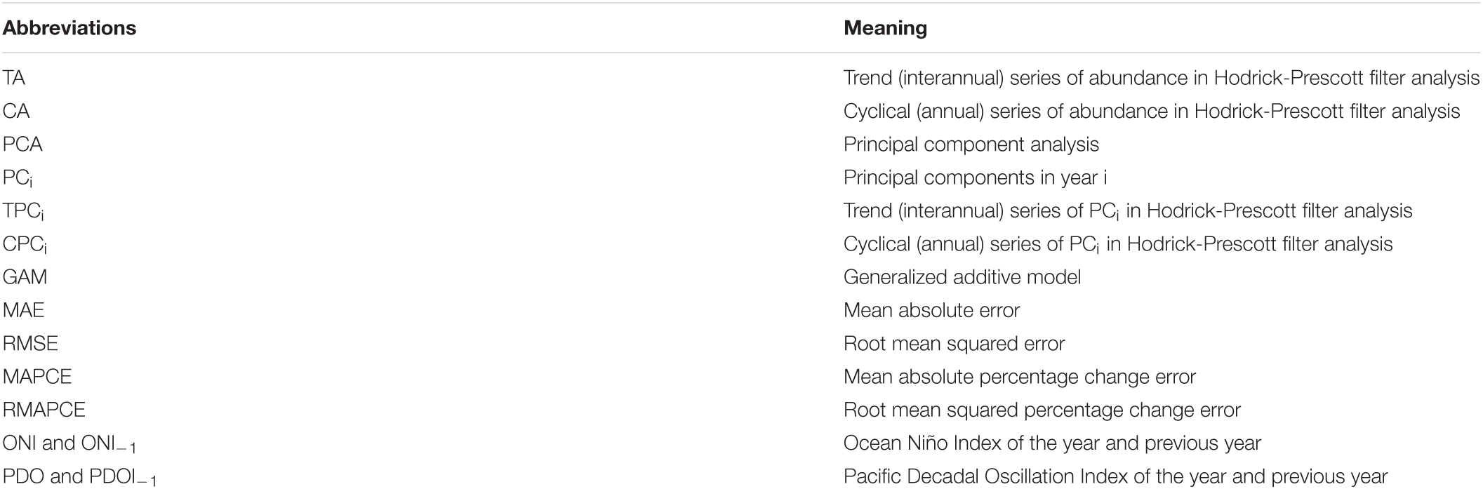
Table A1. Important abbreviations and their meaning.