Effects of Measuring Devices and Sampling Strategies on the Interpretation of Monitoring Data for Long-Term Trend Analysis

Introduction

Measuring changes in water temperature over time is important for assessing climate change impacts. In this context, temperature changes have a fundamental impact not only on the kinetic energy in the system but can also affect the overall cross-taxon structure of marine biodiversity and, therefore, the global distribution of life in the oceans (Tittensor et al., 2010). Because of this central role of temperature in aquatic ecosystem research, regular measurements, especially of surface water temperature, started two centuries ago. Two of the longest near-surface water temperature measurements are a time series from Great Harbor, Woods Hole, Massachusetts, which started in 1886 on a daily basis (Nixon et al., 2004) and a time series from Helgoland in the southern North Sea (54°11.3′N, 7°54.0′E), which started in 1873 with almost daily samples (Wiltshire and Manly, 2004). At these stations, sampling was initially done manually using the traditional bucket thermometer measurement (Nixon et al., 2004), where water was sampled from the near-surface by a simple bucket and temperature was measured immediately with a mercury-in-glass thermometer, with a precision of approximately 0.1°C.

It was only at the end of the last century when watertight temperature sensors became available off the shelf at an affordable price and successively replaced most manual measurement devices. Today, digital temperature sensors are available for most in situ applications, covering a wide range of accuracy and precision (JCGM, 2008), as well as price levels. The rapid development of digital sensor technology not only for temperature but also for most other environmental parameters, as well as the rapid progress in automated sensor technology for automated biota monitoring from lower eukaryotes (Baschek et al., 2017) up to higher trophic levels, such as fish (Fischer et al., 2007), has enabled science to intensify year-round monitoring approaches, even in remote areas. Currently, fully automated monitoring stations are established even in remote areas, such as polar regions, and deliver a continuously increasing amount of environmental information in real-time, year-round (Fischer, 2020). The importance of in situ sensors instead of sea surface measurements derived by satellite and/or model-generated data for coastal regions has been stressed by Smit and Schlegel (2016). They pointed out that remotely sensed gridded sea surface temperature data in coastal waters normally do not approach a sufficient resolution to monitor short-term local changes in temperature as those patterns can be highly dynamic and significantly affected by varying levels of water exchange in lagoons resulting in varying patterns in eutrophication, sedimentation and turbidity. Furthermore, the precision of gridded data is also often too low for climate-quality data to reveal longer-term trends.

Remote in situ measurements of hydrographic and higher trophic level variables opened an entirely new field of technology-driven research in aquatic sciences (Baschek et al., 2017) with the possibility of deriving and testing scientific hypotheses from continuous real-time field observations, which were previously only possible in terrestrial or atmospheric research. However, there are some challenges that accompany these developments, such as sensor maintenance, data flow management, (big) data handling, and data interpretation, that need to be considered (Buck et al., 2019; Fischer, 2020).

In addition to defining specific in situ sensor maintenance intervals, data flow, and handling routines for permanent aquatic monitoring stations, the overall setup of long-term monitoring infrastructure for ecological and climate change-related parameters will determine the scientific output and relevance of such systems and, therefore, long-term financial support. Two of the overall questions that scientists operating sensor-based long-term in situ measurements are confronted with are the required sensor accuracy and precision (JCGM, 2008) and the sampling frequency (Cabella et al., 2019), both of which have a significant effect on the financial requirements of the operations.

According to ISO 5725-1:1994,¹ the term accuracy describes the systematic deviation of a measurement from the “assumed” true value from an accepted reference value (Figure 1).

FIGURE 1

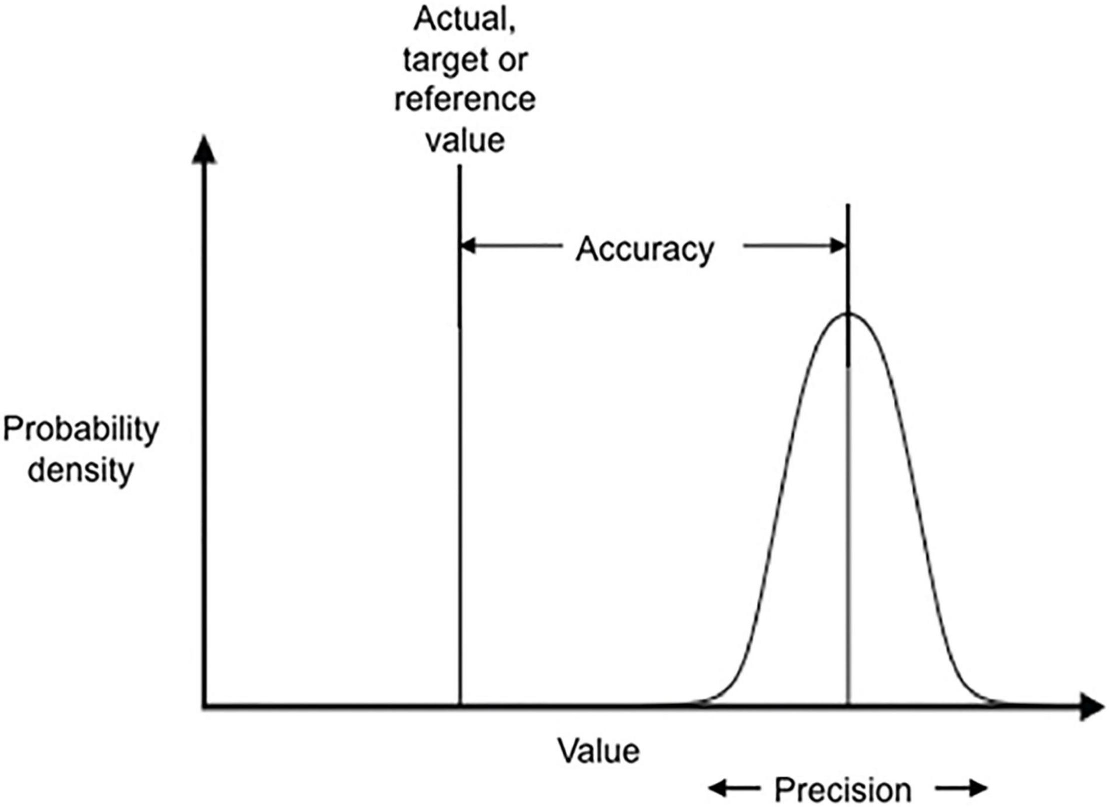
Figure 1. Visualization of accuracy and precision according to ISO 5725-1:1994. The bell-shaped distribution describes a set of measurements of a single parameter (e.g., water temperature) over time with a single sensor or the distribution of synoptic measurements with multiple sensors. Higher measurement accuracy means that the maximum of the distribution moves closer to the reference value. The precision of a sensor refers to the width of the bell-shaped distribution. The more precise a measurement is, the narrower the bell shape of the distribution.

In contrast, the term precision relates to the reproducibility of measurements and their variability between repeated measurements due to, for example, electronic or resolution-based, variabilities of the measurements itself (Figure 1).

Even though both accuracy and precision are defined in their respective ISO standards, the precise meaning of these definitions are debated (Behkamal et al., 2014). For the present work, for accuracy, we strictly followed the definition of ISO 5725-1:1994. This definition is synonymous with the term “semantic accuracy” used in Behkamal et al. (2014), describing the correctness of a data value in comparison to an actual real-world value. In this context, Peralta (2006) defined accuracy as a “semantic correctness factor,” providing the degree of correctness and validity of the data in comparison to the real world or with reference data agreed to be correct. Therefore, when using the term accuracy in the sense of ISO 5725-1:1994, trusted reference data that are assumed to represent the real data must be agreed upon by the sensor user. This trusted data may be either the reference data provided by the manufacturer or it may be trusted reference data provided by the user itself like, e.g., statistically derived mean or median values from multi-sensor approaches or other scientifically convincing procedures agreed upon to deliver “real” values.

Compared to defining a sensor’s accuracy, the calculation of precision seems to be much easier. According to ISO 5725-1:1994, the precision of data depends only on the distribution of random errors around an assumed statistical value, which is, however, not necessarily the true value in the sense of the real value referred to in the above accuracy section. Precision is usually expressed in terms of imprecision and computed as the standard deviation of the measured mean value, which is reflected by a larger standard deviation or confidence limit (ISO/TC-69/SC-6, 1994).

Even though most sensor manufacturers provide lab-derived accuracy values for new sensors, the meaning and consequences of these parameters for in situ measurements are often not completely clear to users in the scientific community. Furthermore, the determination of accuracy and precision often does not follow a common standard. More importantly, the values provided are not the same as in situ, as values significantly depend on factors such as sensor age, exposure time, biofouling, and other external factors (Callow and Callow, 2011; Androulakis et al., 2020).

Therefore, the in situ accuracy and precision values for sensors that are in experimental or operational use in science are usually not well known and are therefore not provided in many scientific manuscripts. However, a reasonable estimate of both values unquestionably improves the likelihood of finding significant evidence if an environmental parameter, for example, changes over time, or if it only fluctuates randomly without a real trend.

In the first part of this paper, we address the issue of sensor accuracy, precision, and comparability of different commercially available temperature sensors within the available price categories between 200 and 15,000 EUR on the potential to measure one or more environmental variables over a certain range as accurately and precisely as possible. Therefore, we conducted laboratory intercomparison experiments to compare the in situ accuracy and precision ranges of different sensors and evaluate the comparability between these sensors. This comparability is particularly important as sensors are replaced after some time, or data from different sensors are analyzed and interpreted together in studies.

In addition to the above-described sensor-specific issues, scientists are often confronted with the decision on how often a sensor should sample per time unit to best assess possible changes and dynamics of a focus parameter. Similar to the above-described issue of accuracy and precision, there are also valid and scientifically proven theoretical concepts to determine an adequate sampling frequency for a certain monitoring task. One of these concepts is the Shannon–Nyquist theorem (Nyquist, 1928), which states that the temporal dynamics of a continuous signal (e.g., the water temperature) of any shape (e.g., daily changes with tide or seasonal dynamics over the year) can be reliably discriminated from random fluctuations only when the sampling frequency is more than twice as high as the frequency of the real signal (Lévesque, 2014). The Nyquist effect can be illustrated by tidal temperature fluctuations in coastal areas. To reliably measure the temperature dynamics in a tidal area with a tide frequency of 12 h for a full tidal cycle, the temperature must be measured at least every 6 h to understand the tidal influence on water temperature. However, this concept holds true only if the underlying signal (in this case, the tide) is strictly continuous with a fixed temporal pattern. An inadequate (too low) sampling frequency may produce deceptive patterns and eventually lead to aliasing effects, and therefore to misinterpretations. Good examples of such misinterpretations resulting from an insufficient sampling frequency in ecological studies are given in Pearcy et al. (1989) based on the Nyquist theorem (Nyquist, 1928). Although these concepts are known in physics and signal processing, most environmental studies do not strictly follow these theoretical concepts when analyzing long-term monitoring datasets. This is simply because ecologically interesting and relevant patterns often only emerge after several years of observations at a specific site and hence, the patterns are not known when initially setting up a monitoring strategy. When reviewing literature on statistical approaches to discriminate real long-term changes in marine or limnic water temperatures from random water temperature fluctuations over time, linear regression over time is one of the most often used methodologies (Taylor et al., 1957; Maul and Davis, 2001; Nixon et al., 2004; Wiltshire and Manly, 2004; Smit and Schlegel, 2016; Niedrist and Füreder, 2020). The main focus of this work is thereof not the requirements of sampling frequency when trying to resolve short-term changes in SSWT, for example, daily or seasonal rhythms, but on the requirements of sampling frequency when trying to discriminate real temperature changes in SSWT from random fluctuations over longer time periods (years) using linear regression.

In the second part of the manuscript, we therefore address the question of how different sampling schemes with different sampling frequency (hourly, daily, weekly, or monthly) affect the observed long-term temperature trend over a period of 5 years. For this analysis, we used a dataset from an Arctic coastal observatory in Svalbard (Fischer et al., 2017; Fischer, 2020) of shallow water temperature changes in the Kongsfjorden ecosystem from 2013 to 2017 (Fischer et al., 2018a,c,d,e,f).

This study is not intended to evaluate or develop standard operating procedures (SOPs) to determine sensor accuracy and precision and not to provide SOPs for the determination of the sampling frequency for a specific monitoring approach as this must be completed specifically for each experimental setup. Rather, the goal of this study is to demonstrate how different sampling schemes with respect to the sampling frequency and use of sensors with different accuracy and precision values can affect the outcome of monitoring programs. The results are thus discussed considering: (1) the requirement to select suitable sensors for long-term oceanographic measurements, including cost-benefit considerations when using either expensive oceanographic sensors, such as CTD or thermo salinometers, compared to multiple relatively cheap temperature sensors that are available off the shelf and (2) the possible effects of different temporal sampling schemes on the results. The latter considerations are essential when deciding how much money and workforce should be invested for a long-term sampling program to detect relevant changes in the target parameter (here water temperature) with high reliability and accuracy without exaggerating the sampling and data handling efforts.

Materials and Methods

To test the influence of different sensors and sampling strategies to observe a specific environmental parameter over longer periods of time, we used the variable water temperature as it is the most important hydrographic variable across the aquatic disciplines in the context of climate change (Tittensor et al., 2010). In two approaches, in vitro and in situ setups, standard aquatic temperature sensors with different manufacturer specifications for accuracy and precision were used (Tables 1, 2).

TABLE 1

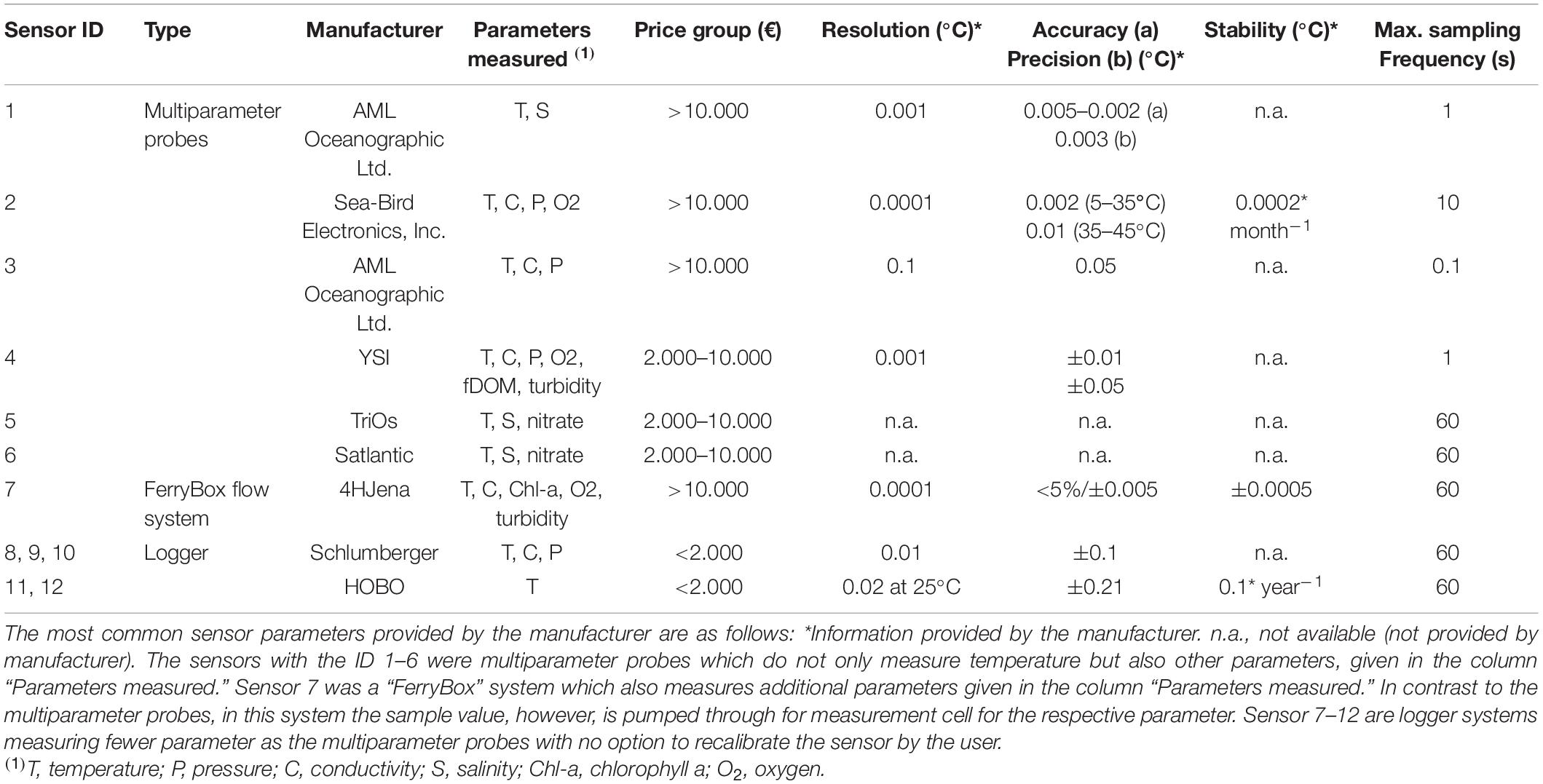
Table 1. Sensor analysis in the intercomparison experiment.

TABLE 2

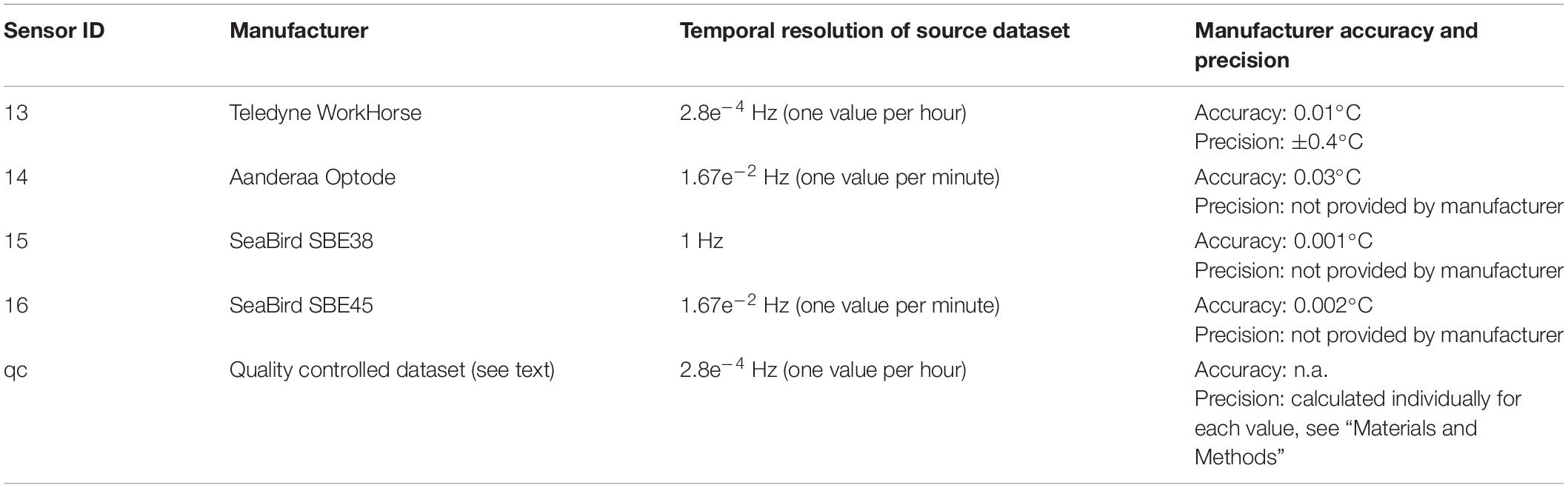
Table 2. Sensors, respectively, datasets available for the in situ approach.

In vitro Experiments

For the in vitro experimental setup, a 24 h experiment was conducted as a joint experiment comprising the five Helmholtz Institutes Alfred-Wegener-Institute, Helmholtz-Centre for Marine and Coastal Sciences (AWI), Hereon (HZG), Helmholtz-Zentrum für Ozeanforschung Kiel (GEOMAR), Helmholtz-Zentrum für Umweltforschung (UFZ), and Deutsches GeoForschungsZentrum (GFZ) within the framework of Modular Observation Solutions for Earth Systems (MOSES) (Weber et al., 2021). The main goal of the experiment was to compare different sensors as they came from different cooperating research institutes, which are often involved in comparative measurements during joint field campaigns. Thereby, the main focus of the here presented experimental approach was, if the different sensors provide comparable results and not the numerical deviation of the single sensors from an assumed “true” value. This latter topic can only be addressed in a certified sensor calibration lab under strictly controlled conditions.

In the in vitro experiments, 14 different temperature sensors continuously measured the seawater temperature in an experimental tank of 100 cm × 60 cm × 100 cm (600 L). The sea water temperature in the tank was gradually lowered from 18.8 to 15.8°C within a period of 13 h (Figure 2) by continuously adding freshwater of a constant temperature of 15.8°C. Complete mixing in each basin was ensured owing to the circulation circuit. Parallel rails were installed above the basins and the sensors were deployed from them in the basin at the same depth of 60 cm. The sampling frequency of each sensor was set according to the sensor manuals to the highest frequency possible for the sensor [Table 1, column “Max. Sampling Frequency (sec)”], as this is, to our experience, the most applied sampling frequency set-up in operational science.

FIGURE 2

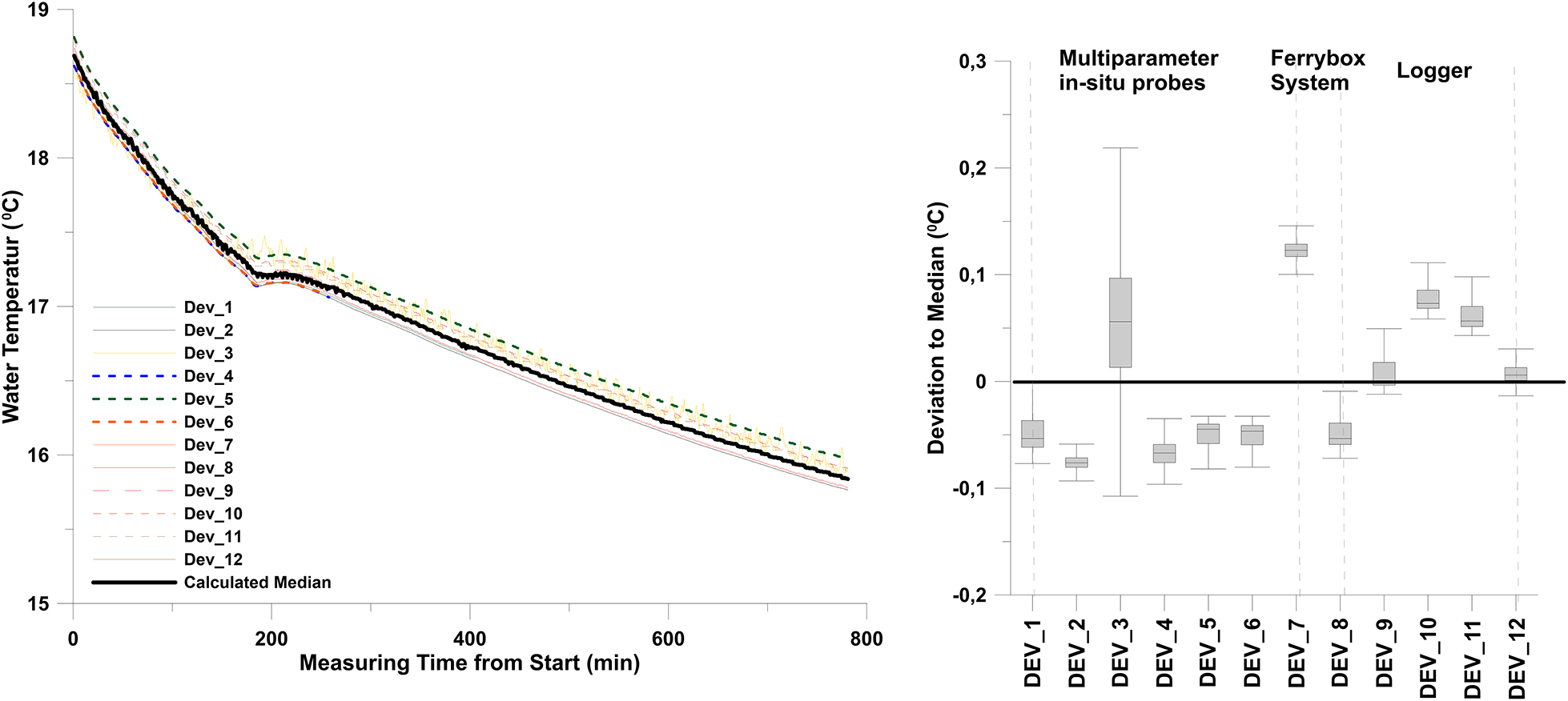
Figure 2. Water temperature over time in a water basin for all of 12 sensors (inbox). Deviation to the calculated median (°C).

For the data analysis, all data were averaged over 1 min to reduce the bias toward sensors with a higher sampling frequency. As the experiments targeted the interoperability of the sensors, we used the median temperature of all 14 sensors as reference data for each time step.

The sensors included low-cost water temperature data loggers, water level loggers, instrument clusters, such as CTD probes, and flow-through systems, such as FerryBoxes (4H Jena Engineering GmbH). These sensors represent a price range between 200 and 15,000 EUR. The measurement principle of the different sensors varied with different resolutions and accuracies (Table 1). The sensors are usually applied to a wide range of environmental research questions covering ground water, fresh water, coastal, and marine compartments.

Pre-experiment sensor handling followed standardized routines defined by the sensor manufacturers and individual routines. All sensor operators prepared their sensors exactly, as they normally do for standard scientific missions. Specific across-institute concerted sensor preparation procedures were explicitly not provided, as we wanted to focus on possible variations of measurement between different standard sensors under SOPs as applied by different scientific operators and institutes. Therefore, we did not provide any guidelines with respect to sensor calibration and routine maintenance prior to the experiment, except that the routines must be in full agreement with the respective institute guidelines for good sensor handling practice prior to scientific measurement campaigns.

In situ Data

Study Site and Sensors

As an in situ dataset for evaluating the effects of different sampling frequencies, we used a dataset from January 01, 2013 to January 31, 2017 from the Svalbard AWIPEV observatory close to the Arctic research settlement in NyÅlesund (Figure 3).

FIGURE 3

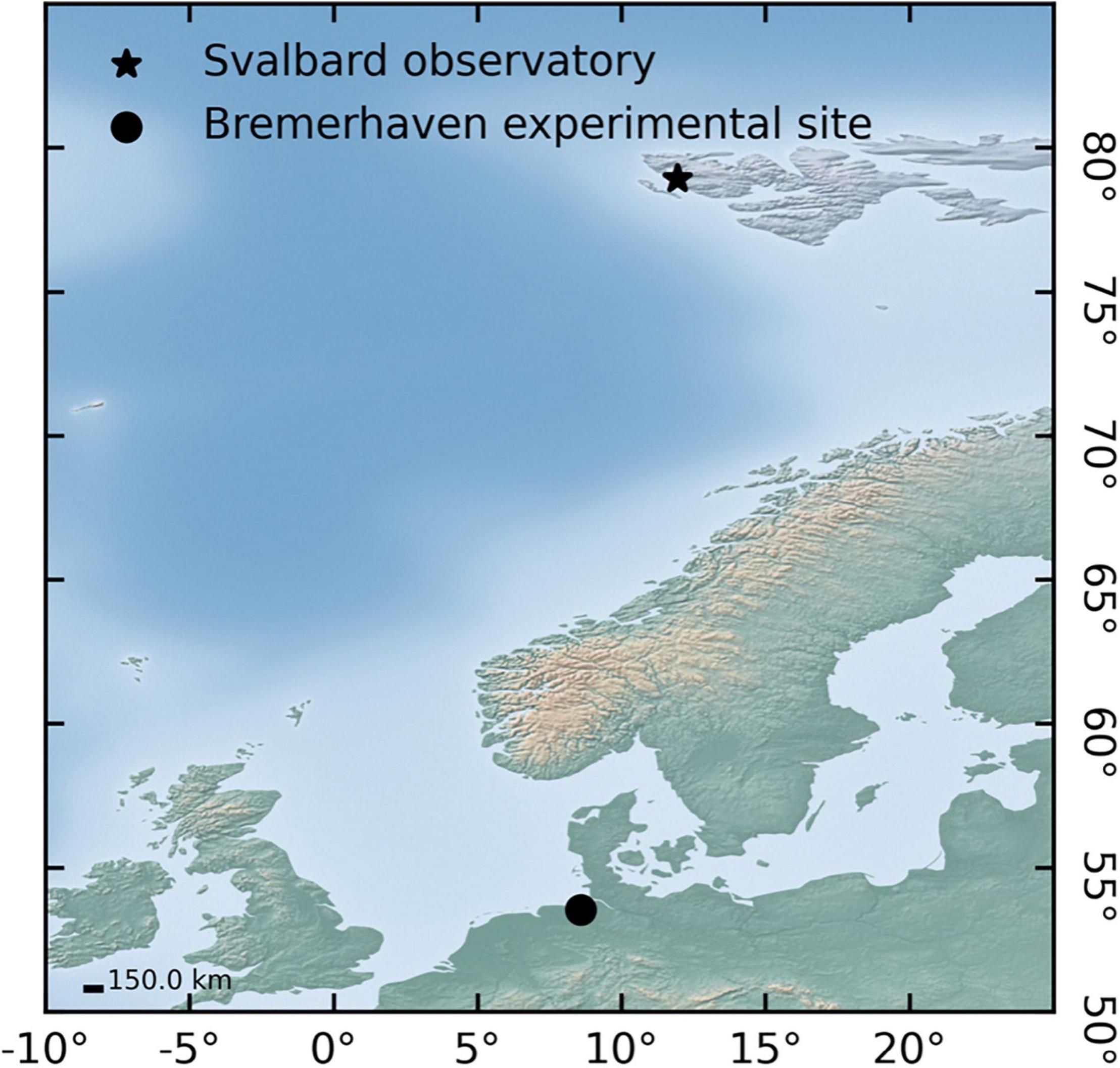
Figure 3. Location of the Bremerhaven experimental site for the lab experiments and the COSYNA observatory in the Arctic Ocean, Svalbard archipelago (78.93045°N, 11.9190°E), base map: Natural Earth (2018).

The dataset comprised temperature data from four different sensor types (Table 2) measuring the water temperature year-round at a frequency of 1 s^–1 to 1 h^–1. The sensors were placed a maximum of 1.5 m apart in a water depth of 11 m to 12 m ± 1.5 m tidal cycle and were operated continuously except during maintenance and repair.

Overall Data Treatment

The data flow and handling of the raw data from the Svalbard observatory is described in Figure 4 using R (R Core Team, 2021a,b) with the packages listed in Supplementary Appendix 1. For the analysis, we used raw datasets from four different sensors on which plausibility checks according to Silva et al. (2020) were applied, classifying the data into good, probably good, probably bad, and bad data (Figure 4, step 1). In the next step (Figure 4, step 2), all data were visually inspected on a monthly basis using an interactive Shiny (Chang et al., 2021) application in R programming language (R-Studio Team, 2020). The data point plausibility classification from step 1 was confirmed based on expert knowledge. Data points that were obviously wrongly classified as “good” were manually classified as “probably bad.” The output of this step was used as single-sensor plausibility-checked datasets for further analysis.

FIGURE 4

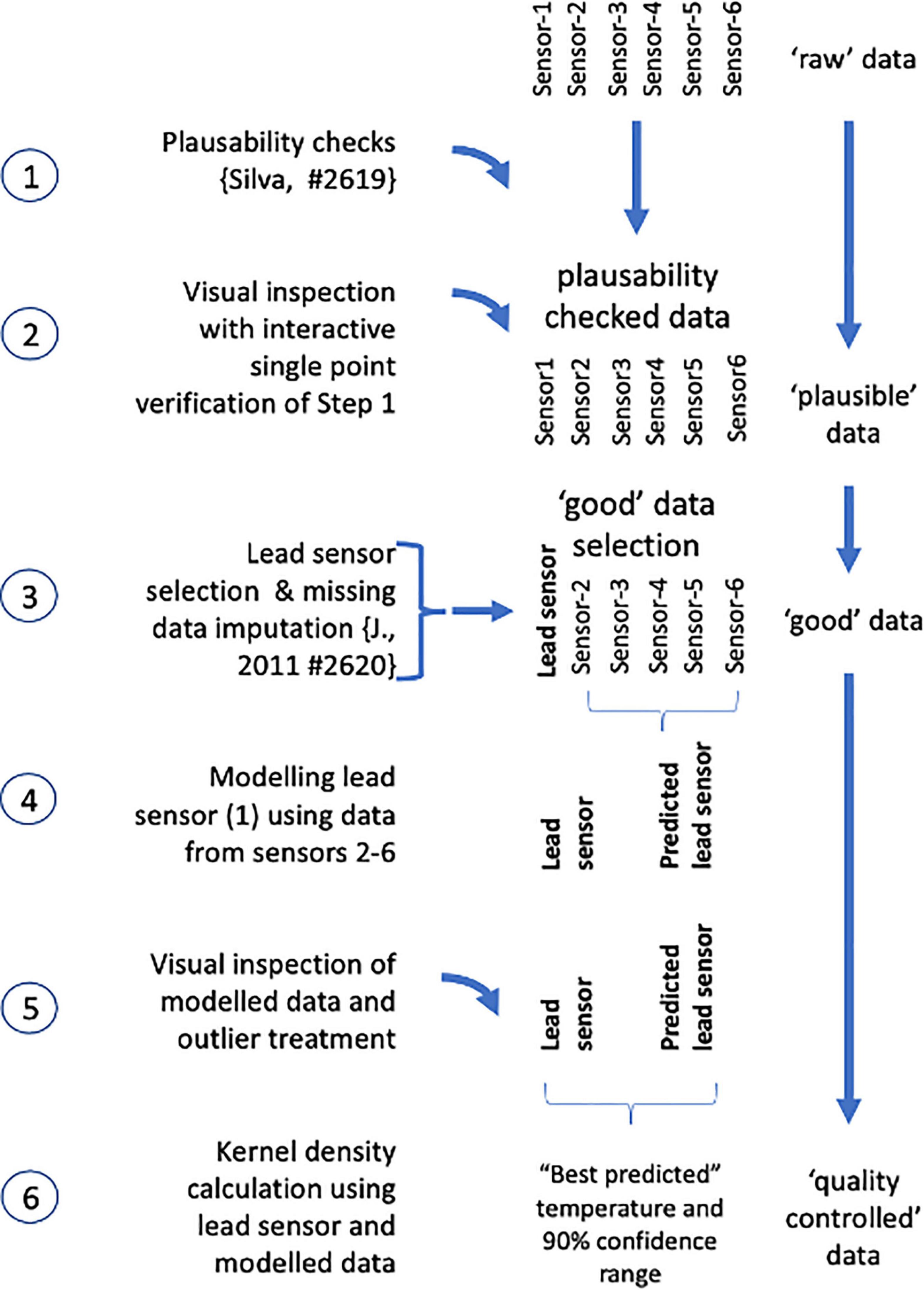
Figure 4. Data flow and handling from single sensor raw data sets to quality controlled data. Further explanations see text.

Quality Controlled Data Set

Additionally to the single sensor datasets, quality controlled datasets from 2012 to 2017 were used which have been published as yearly datasets in the Pangaea data repository (Fischer et al., 2018b,c,d,e,f,g). Similar to the approach described by Henson et al. (2010), for multiple satellite models targeting the same parameter, we derived an integrated temperature dataset from the single-sensor datasets described above. From these datasets, the sensor with the highest manufacturer accuracy and precision, the least obvious outliers, and the lowest temporal drift in the plausibility check procedure (Figure 4, steps 1–2) was defined as the lead sensor. Missing data in this lead sensor were imputed as far as possible (Figure 4, step 3) using the imputation routine “Amelia” from the R package Amelia II (Honaker et al., 2011). In the next step, using multiple linear regression, a model for predicting the lead sensor values was applied using the other sensor data as predictors (Figure 4, step 4). Using this model, an as complete as possible dataset “predicted lead sensor values” was created. The lead sensor and predicted lead sensor data were then analyzed with respect to their goodness of fit by computer-aided analysis (Figure 4, step 5). In this step, the residuals of the fitted to lead sensor values were calculated and visually inspected. Lead sensor values and associated predicted lead sensor values with a numerical difference of more than 3 × studentized standard deviation of the lead sensor were classified as probably bad. Using the remaining “good” data of the lead sensor and the associated predicted lead sensor, kernel density estimates (for details, see Deng and Wickham, 2014) were calculated (Figure 4, step 6). A kernel weight value of 1 was used for the lead sensor value. For the associated predicted lead sensor value, a kernel weight value of 0.7 was applied. Based on these parameters, the kernel maximum values and their 90% confidence limits were calculated as the assumed best fit for the in situ mean temperature and the associated 90% confidence limits of the mean temperature at a certain time. This dataset is referred to as “quality-controlled dataset” in all subsequent steps.

For all further calculations, both the four single sensor data sets and the quality-controlled dataset were averaged (arithmetic mean) per hour so that mean hourly temperature data were available.

Virtual Sampling Campaigns

Using these five time series, virtual sampling campaigns were conducted from 2012 to 2017, simulating a realistic monitoring program on SSWT in the Arctic. When setting up the sampling frequency and procedure, we used our experiences of long-term sampling programs with logistic support available on year-round operated polar field stations. Based on these considerations, the five source datasets with temporal resolutions of 1 h were sampled in silico in four different temporal scenarios: full hourly resolution, sampling once every day, once every week, and once every month. As stated before, to follow as best as possible a realistic field sampling scenario, sampling in the daily, weekly, and monthly scenarios was performed during the workday between 10:00 and 15:00. Within the temporal scenarios daily, weekly, and monthly, three different sampling sub-scenarios were performed (Table 3). All calculations and routines for the in silico sampling were done in R-Studio (R-Studio Team, 2020) and are available as R notebook at Github (Supplementary Appendix 1; Fischer, 2021).

TABLE 3

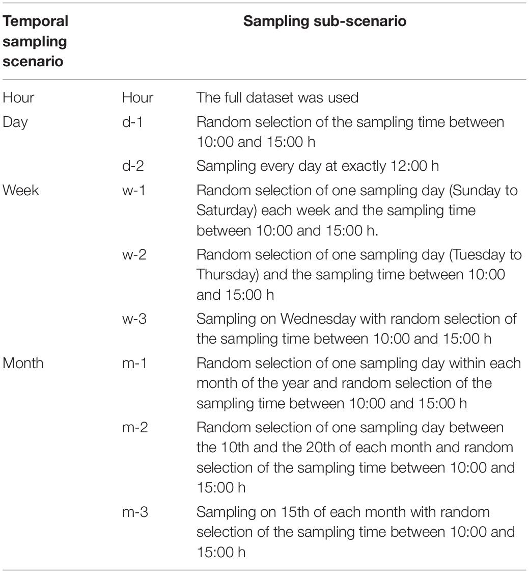
Table 3. Overview of the temporal (hourly, day, week, and month) sampling scenarios in the in silico sampling procedure.

In the d-1 scenario, sampling was performed every workday year-round with a random selection of the exact sampling time between 10:00 and 15:00 every day. In the daily d-2 sampling scenario, sampling was also performed every workday, but exactly at 12:00.

For the different weekly sampling scenarios (Table 2, w-1 to w-3), one sample was taken per week either on any day of the week (w-1) including Saturday and Sunday, only from Tuesday to Thursday (w-2), or only on Wednesday (w-3). In the weekly scenarios, the exact sampling time per day was always randomly selected between 10.00 and 15:00.

For the three-monthly sampling scenarios (Table 2, m-1 to m-3), one sample per month was performed either on any day of the month (m-1), only between the 10th and the 20th of each month (m-2), or exactly at the 15th of each month (m-3). As in the weekly scenarios, the exact sampling time per day was randomly selected between 10.00 and 15:00 h.

Applying this sampling strategy, nine different virtual sampling scenarios (Table 3) were analyzed using a comparative approach. All five datasets (Table 2, sensor ID 13-17) were analyzed with respect to significant temperature changes over time from January 2012 to December 2017 and their potential to detect significant changes over time.

Data Analysis

All analyses were performed with R-Studio (R-Studio Team, 2020) and Python, and the packages are listed in Supplementary Appendix 1. For the in vitro experiments, a Bland–Altman analysis was performed to evaluate the agreement between the two series of measured values. In particular, it provides information about the influence of the height of the measured values on the magnitude of the deviations/differences. The Bland–Altman analysis is based on the quantification of the agreement between two quantitative measurements by determining the bias or mean difference as a measure of accuracy and construct limits of agreement (LOA) as a measure of precision (Altman and Bland, 1983; Bland and Altman, 1986). This is used to evaluate the agreement between two different instruments or two measurement techniques (Montenij et al., 2016). For the in situ and in silico analysis of temperature changes in water temperature in Svalbard over time, we applied ANOVA with subsequent linear regression analysis (temperature versus time). For all virtual samplings where the possibility for a random choice of the sampling hour, day, or week was given (all sampling schemes except for hour and d-2), 100 computer-generated repetitive samplings were performed. For sampling scheme w-2, for example, the computer conducted 100 (virtual) repetitive samplings with a random choice of sampling day (Tuesday, Wednesday, or Thursday) and sampling hour (between 10:00 and 15:00). The results of these 100 samplings were used as input variables for subsequent statistical tests on the effects of the parameters “sampling time,” “sensor-id,” and (in silico) “replicate sampling” on the possibility of detecting an increase in water temperature over time. Furthermore, the 100 slopes of the “samplings” were used to calculate the predictive capacity of a significant increase in temperature over time.

Results

In vitro Data

In addition to evaluating the comparability of the tested sensors with respect to sensor accuracy and precision, we also evaluated whether specific sensors may be more appropriate for scientific tasks based on measurement characteristics. We specifically checked if there were sensors that were more appropriate for (1) measuring the “true” temperature as accurately as possible or (2) determining minimal small-scale temperature changes over time. While task (1) has less strict requirements regarding the accuracy of the measurements, task (2) requires a high precision of the temperature measurements.

The median of all sensor data for each time step was determined to analyze the accuracy of the different sensors within the intercomparison experiment. Usually, sensor accuracy is calculated using a “true” value. However, measurements of the true value are extremely challenging, and reference techniques can only provide an approximation. In this set-up, the real “true” temperature was unknown. Therefore, the difference between each measured data and the calculated median at each time step was determined. Figure 2 displays the temporal behavior of all the sensors and the deviation of each sensor to the calculated median. Figure 2 indicates that data from all multiparameter probes were below the median value, except for DEV_3. In addition, FerryBox revealed warmer temperatures. The loggers’ water temperatures were either very close to the median value or above the median value. DEV_8–DEV_10 were of the same type, but DEV_8 measured colder than the median water temperatures, while DEV_3 and DEV_10 measured higher water temperatures, indicating a high variability of this type of sensor.

As described above, one aim was to find reasonable and feasible metrics to select the most appropriate sensors for a specific scientific task. It is essential to be certain that the sensor of interest is as accurate as a reference or as an assumed “true” value. Therefore, it is crucial to measure the agreement between the two sensors.

One approach to evaluate the agreement is using Bland–Altman analysis between two sensors, rather than validating the sensors to a “true” reference. Bland–Altman analysis is based on quantifying the agreement between two quantitative measurements by studying the mean difference and constructing the LOA (Giavarina, 2015). The LOA is a confidence interval, and it is commonly computed by ±1.96 × standard deviation of the difference for each comparison. LOA describes how far apart the measurements of two methods are likely to be for most individuals. Here, Bland–Altman analysis was performed using the median of all sensors as a reference to determine the mean accuracy (bias) (Figure 5). The Bland–Altman diagram in Figure 5 shows the differences between each measuring device (DEV), the median of all sensors (REF) on the Y-axis (DEV − REF), and the mean of these two parameters [(DEV + REF)/2]. Figure 5 shows that the means are different for a bias = 0. A bias close to zero indicates an accurate sensor. The sum of the distance of the upper and lower LOAs to 0 indicates the precision (Figure 5).

FIGURE 5

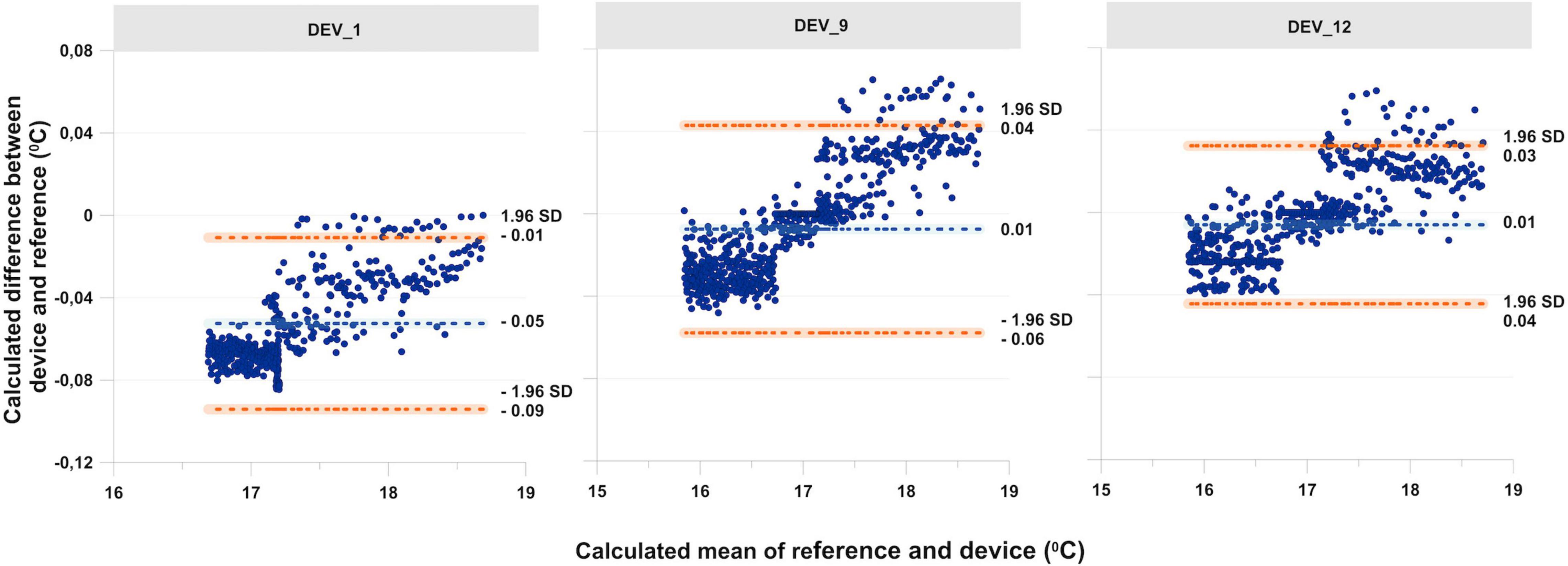
Figure 5. Example of Bland–Altman analysis taking the median of the reference sensor and three different sensors (DEV_1, DEV_9, and DEV_12) and the calculated reference as the median of all sensors; the light blue stripe indicates the mean difference of the device to the reference and represents the bias. The two orange bars represent the confidence interval at 95%.

In Figure 5, it can be seen that the sensors are precise if the limits are close to the bias. In this example, DEV_9 was the most accurate and DEV_12 was the most precise in relation to the median.

These percentage differences between the reference and the sensor show that mean accuracy is the best benchmark to find the sensor that measures the temperature as accurately or “true” as possible. In Figure 6, the results indicate that within the intercomparison experiment, DEV_7 (FerryBox System, in Figure 6A1) and DEV_12 (logger, in Figure 6A2) are the most appropriate. In addition, parameter precision is suitable for selecting repeatable sensors and can record small temperature changes. For the latter research questions (resolving small temperature changes), DEV_6 (Multiparameter in situ probe, in Figure 6P1), DEV_11, and DEV_12 (Logger, in Figure 6P2) should be selected.

FIGURE 6

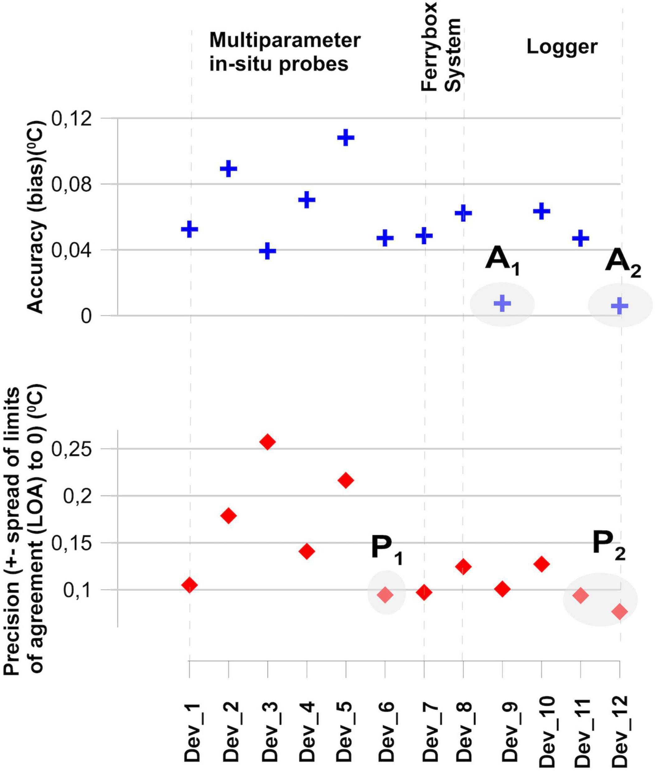
Figure 6. Percentage difference between sensor and reference from the Bland–Altmann analysis: (upper panel) bias or mean difference as a measure of accuracy, if bias >0 then median >sensor and, as a result, the median provides a bigger retention than the sensor and vice versa. A1–A3 are the most suitable sensors for accuracy estimates; (lower panel) spread of limits of agreement (LOA) to 0 as a measure of precision, P1–P2 are most suitable sensors for precision estimates.

In situ Data

Figure 7 shows the base datasets of water temperature of the Svalbard AWIPEV underwater observatory from 2012 to 2017 of the four single sensors and the quality-controlled data set. The statistical analysis revealed a highly significant increase (p < 0.001, lower right panel, column significance slope) in water temperature over time for all five datasets, with a numerical range of the temperature increase between 0.14 and 0.33°C year^–1 (lower right panel, column slope).

FIGURE 7

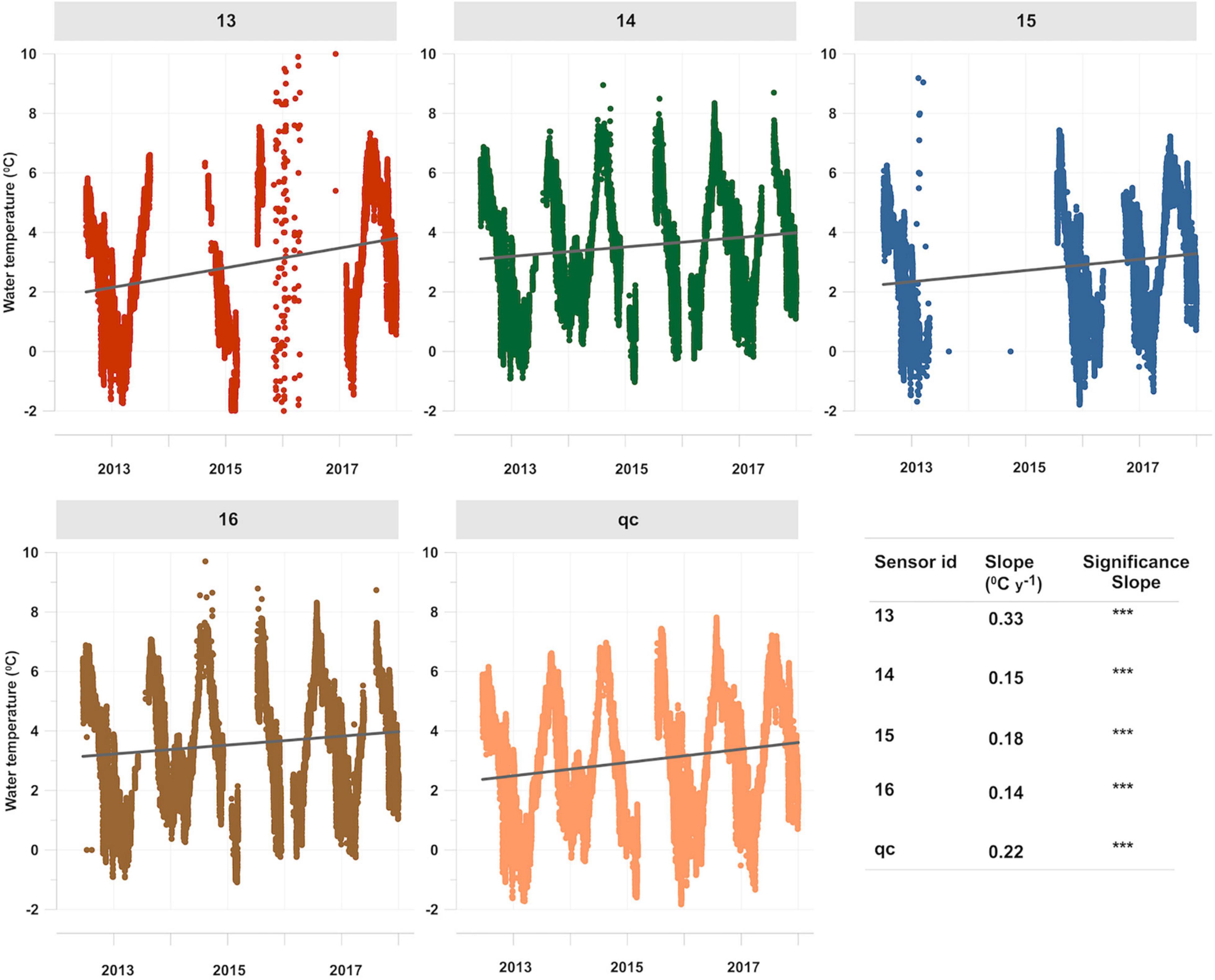
Figure 7. Water temperatures (temporal resolution 1 h) of the Svalbard AWIPEV underwater observatory from 2012 to 2017 for the four single sensors and the quality controlled data set. In each plot, the available data of each sensor are shown after applying the plausibility control procedure (Silva et al., 2020). Additionally, the linear regression fit for each sensor is plotted and the respective numerical slope value and slope significance class are shown in the lower right facet. ***p < 0.01.

This basic dataset (subsequently referred to as an “hourly” dataset) was used for all subsequent virtual sampling campaigns. Table 4 shows the results of hourly, daily, weekly, and monthly sampling schemes, as well as the effects of a very strict sampling plan with no free choice of the hour or day of the sampling versus a liberal sampling plan where the station personnel (here the computer) can schedule the hour or the day of the sampling within the predefined range according to their wishes.

TABLE 4

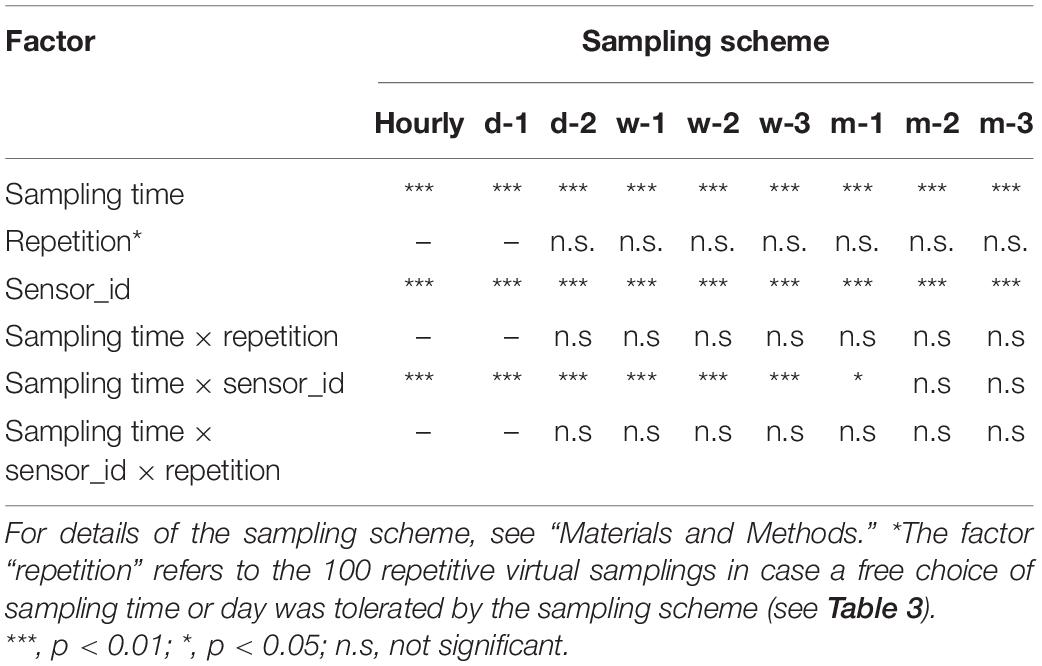
Table 4. ANOVA results on the statistical effects and interactions of the parameters “sampling time,” “sensor-id,” “repetition,” and “sampling scheme” on the increase of water temperature per year (slope).

The results in Table 4 show that in all sampling schemes, “sampling time” and “sensor id” had a significant effect on the temperature measurements. In contrast, “repetition” had no significant effects. Furthermore, the interactions between “sampling time × sensors_id” were highly significant (p < 0.01) for hourly, daily, and weekly sampling schemes, indicating that for these sampling frequencies, the measured temperature change (slope) over time was significantly different among the different sensors.

However, when sampling monthly, this difference between the sensors over time could only be resolved with the restricted sampling scheme when the monthly sampling was performed exactly on the 15th of each month (m1) over the entire time period and only with p = 0.05. In contrast, when sampling monthly with the “half” or “full” sampling scheme (m2, m3), no significant interaction between sampling time and sensor was observed.

Finally, the interaction term including the factor replicate (time × repetition as well as time × sensor × repetition) was not significant in any sampling scheme, indicating that the random selection of the sampling time or day in the 100 virtual sampling events within each time slot did not confound the analysis with respect to hidden temporal patterns introduced by the sampling scheme.

Figure 8 shows the predictive capacity of the different sampling schemes in detail. For this analysis, 100 replicate samples within one sampling scheme (d1, d2, w1, w2, w3, m1, m2, m3) were analyzed. The percentage of 100 repetitive samplings in each sampling scheme was calculated to detect the temperature increase over time with the same significance level as that found in the hourly sampling.

FIGURE 8

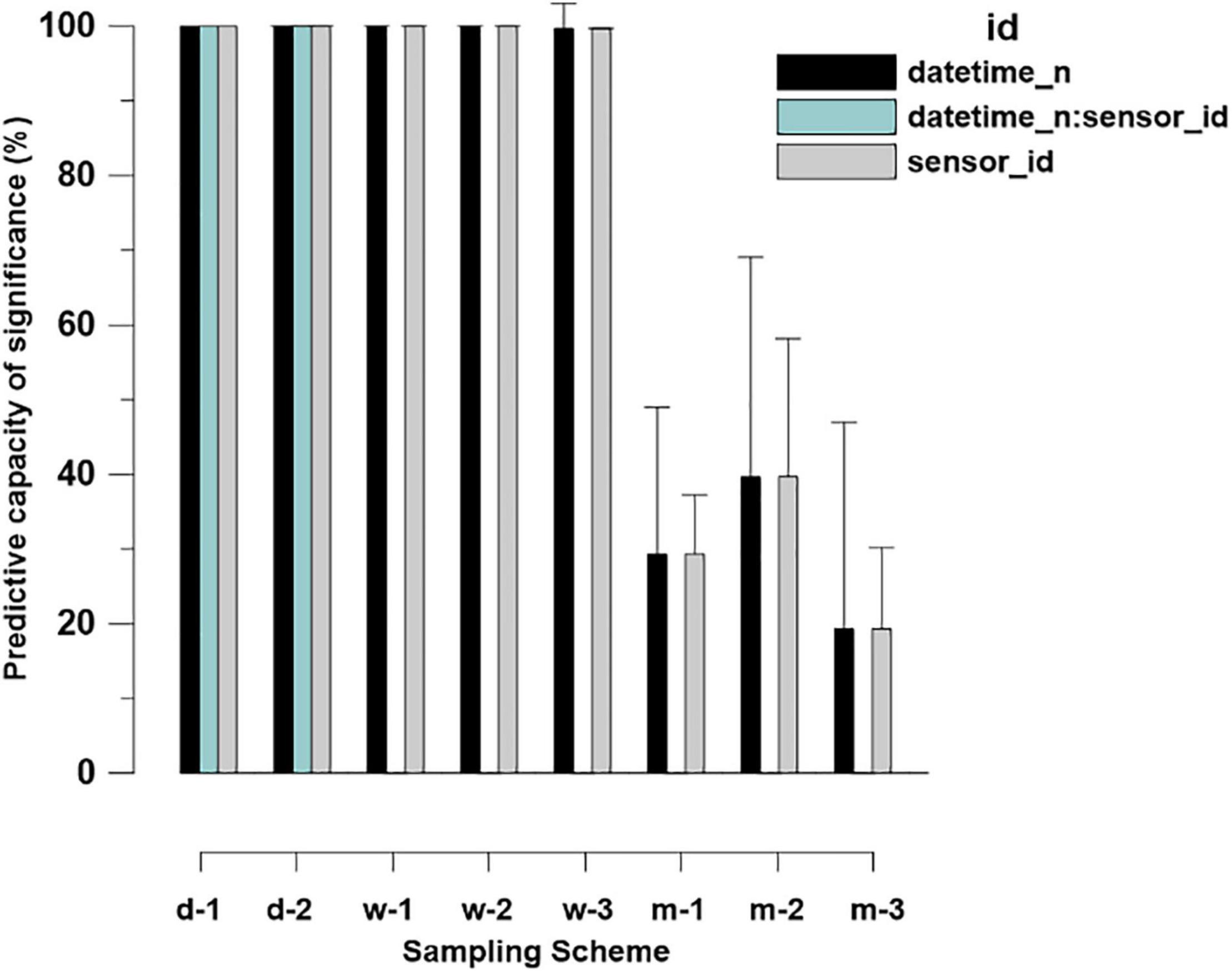
Figure 8. Predictive capacity of different sampling schemes compared to hourly sampling. Hundred percent predictive capacity means that all 100 virtual repetitive samplings within a sampling scheme detected the significance in temperature increase over the period found in the hourly sampling. Zero percent predictive capacity means that none of the 100 virtual samplings within a sampling scheme detected the significant temperature increase over the period.

Our analyses show that daily sampling (either full random or restricted, d1, d2) revealed identical results as hourly sampling for all sensors and sampling times, and for the interactions between sampling time and sensor ID.

Weekly sampling was similar except for the interaction term “sampling time × sensor_id.” For this interaction term, the predictive capacity dropped to 0% in the weekly restricted sampling scheme. This shows that only daily sampling allows statistical disentangling of the effects of sampling frequency on the effects of sensor type when analyzing temperature increase over time.

When switching to the monthly sampling scheme, the predictive capacity dropped sharply. This means that with this sampling scheme, it is no longer possible to reliably determine the temperature increase over time from undirected signal noise. In the 100 repetitive samplings, a statistically significant relationship between temperature increase and time was found in only 40%, and the effect of the different sensors on the temperature measurements was found to be less than 20%.

In the next step, we analyzed the temperature measurements of each sensor in detail to focus on the effects of using different sensor types to determine long-term temperature changes (referring to the factor “sensor-id” and “sensor-id × sampling time” in the above analysis). Figure 9 shows the calculated mean temperature increase per year (slope) measured with the different sensors from January 2013 to December 2017 for the individual sampling schemes. Additionally, the standard deviations of the slope measurements of the 100 replicate samplings within each sampling scheme are shown. The analysis revealed that the temperature increases per year (slope) measured by the individual sensors were quite different. The highest temperature increase per year was detected by sensor 13 with an average increase of 0.34°C per year, a minimum value of 0.31°C (±0.08°C), and a maximum value of 0.39°C per year (±0.01°C). With all daily and weekly sampling schemes, the temperature increase measurements of this sensor were significantly higher (p < 0.001) than those of all other sensors. When the sampling frequency dropped to monthly, this difference was no longer significant, and the p-value between the sensors dropped to 0.05 (Table 4), even though the numerical differences in the temperature increase measurements of this sensor to all others were still obvious.

FIGURE 9

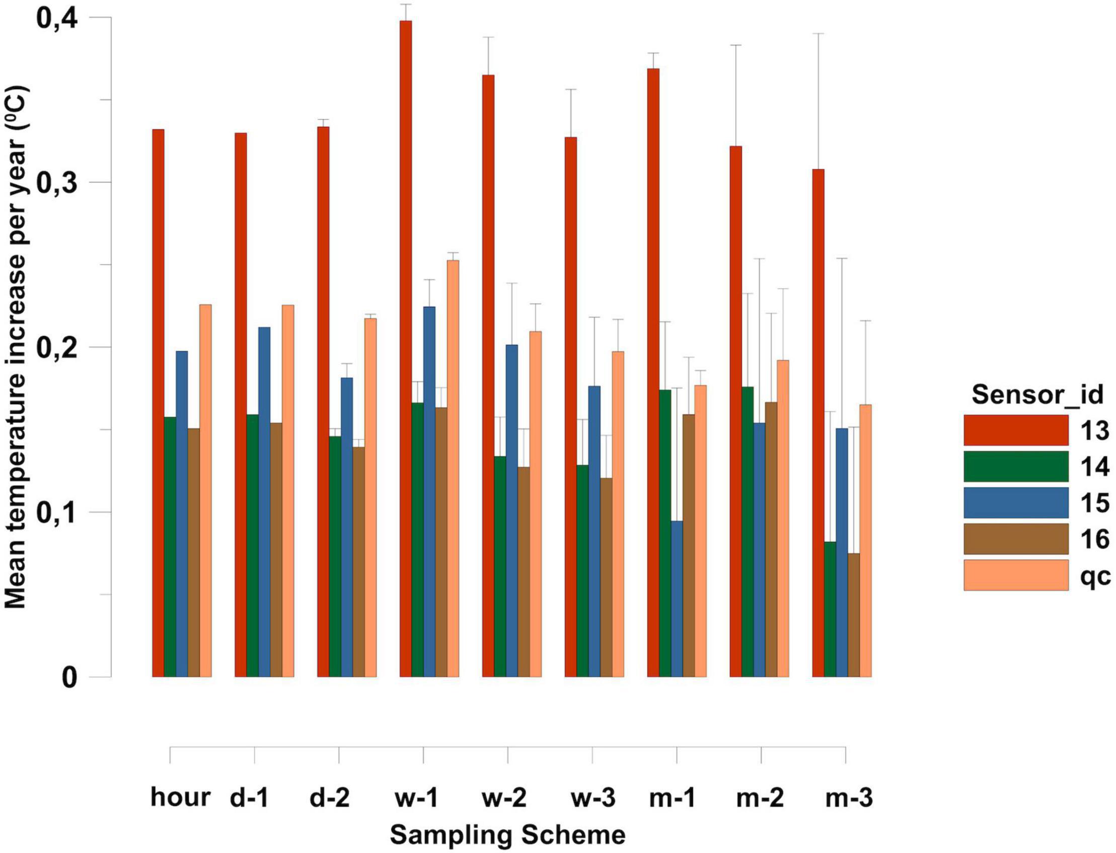
Figure 9. Calculated mean temperature increase per year (slope) from January 2013 to December 2017 measured with the different sensors. Shown are the mean slope values calculated from 100 virtual replicate sampling within the individual sampling schemes. Additionally, the standard deviations of the slope measurements are shown as whiskers.

In the last step, which is identical to the calculation of the predictive capacity of the different sampling schemes, we calculated the predictive capacity of each individual sensor to discriminate a real increase in water temperature over time from random temperature fluctuations (Figure 10). This analysis revealed that when using a single sensor, reliable determination of real temperature increase over time (100% detection) from random temperature fluctuations was only possible with hourly and daily sampling schemes. When switching to weekly sampling, the predictive capacity dropped in almost all sensors to a value of only 50% in the validated dataset, most sensors were even below 40%. A higher value above 90% predictive capacity was only shown by the ADCP temperature sensor, which, however, showed significantly higher temperature increase values than all other sensors. When finally switching to a monthly sampling scheme, the predictive capacity of all sensors approached values was close to or at 0.

FIGURE 10

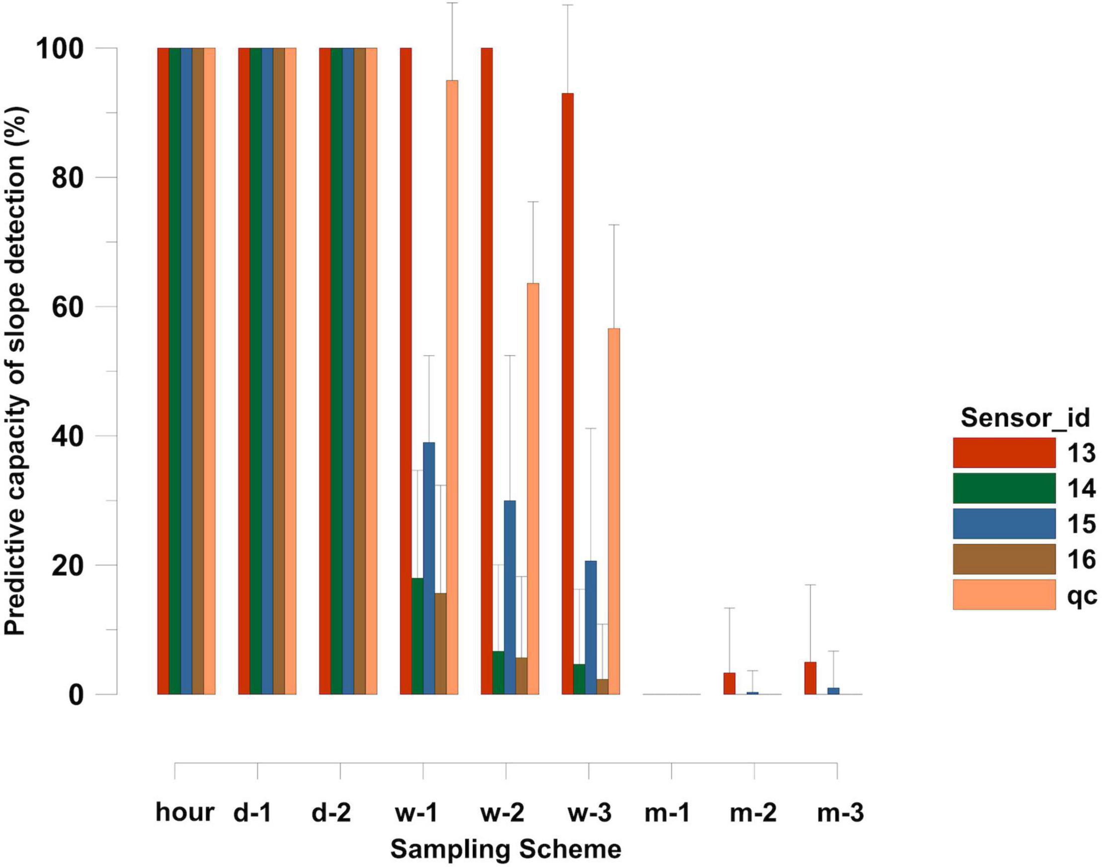
Figure 10. Calculated mean temperature increase per year (slope) from January 2013 to December 2017 measured with the different sensors. Shown are the mean slope values calculated from 100 virtual replicate sampling within the individual sampling schemes. Additionally, the standard deviations of the slope measurements are shown as whiskers.

Discussion

Best practices and standards for aquatic monitoring have gained increasing attention in recent years (Buck et al., 2019; Pearlman et al., 2019). These discussions are highly valuable and are required for setting up theoretical frameworks to achieve good and FAIR data (Wilkinson et al., 2016), especially for longer lasting monitoring programs.

According to our experiences, however, such frameworks are sometimes not written in an operational way to allow easy implementation in a concrete data workflow and, therefore, are not used to their full effect in the ecological community. The sometimes high level of abstraction prevents the implementation of the often well-designed but theoretical procedures in the data workflow, meaning that they do not make their way to operational science as scientists are not able to adapt the suggested procedures to their specific scientific application. These problems in the translation process from theoretical data quality considerations to operational science can be observed at many levels of operational monitoring and, unfortunately, sometimes prevent the comprehensive implementation of described workflows on data quality in operational scientific work.

In vitro Data

Our results from the in vitro experiments show that the simple formula of “the more expensive a sensor is, the better is the data quality” does not hold true. The intercomparison experiment showed that the sensors used in the experiment span from sensors with a high accuracy but a lower precision (example DEV 3) to sensors with a lower accuracy but a higher precision (DEV 6). Most interestingly, these sensor characteristics were not linked to the sensor’s cost. A sensor with a high accuracy means that the sensor measures are highly accurate with a low deviation from the expected temperature. On the other hand, a sensor with high precision can discriminate small-scale temperature changes even though the absolute measured temperature may deviate from the expected temperature more than in the highly accurate sensor (JCGM, 2008). This discussion, however, becomes highly complex especially when approaching the resolution limit of a sensor. In this operational limit, it is almost impossible to decide if small-scale temperature variations detected in a highly precise but less accurate sensor are the result of real changes in the field, or simply accuracy deviations generated in the sensor itself. The rule of thumb could be that any validation of small-scale variations in water temperature should be larger than the known accuracy deviation of the particular sensor in question. Following this argumentation, the precision of a sensor becomes a relative value that depends also on its accuracy. The best choice to obtain climate-quality SST data for instance would be to have both, a highly accurate as well as highly precise sensor. These theoretical considerations clearly show, that additional to comparative and more operational experiments, as performed in this study, in depth benchmark studies for each type of sensor are very useful and required for researchers to make a choice according to their available budget and objective of the measurements (e.g., short-term local variations versus long-term global trends across a range of sites).

The sensor systems used in our intercomparison experiment varied in measurement technique and price, from high-end FerryBox systems and multiparameter in situ probes to low-cost single-parameter temperature loggers. Depending on the scientific question and the local circumstances, scientists need to decide whether a single expensive sensor with long-term high frequency logging and multi-parameter measurement options is more appropriate for their program than multiple cheaper sensors or exchanging sensors every month when cheap sensors are available with similar or sufficient sensor accuracy and precision. For instance, the low-cost loggers of HOBO (DEV 11 and 12) measured the temperature during our intercomparison experiment with good accuracy and precision.

Another remarkable finding of the intercomparison experiment was that the behavior of each sensor is sensor-specific, and even sensors of identical type and manufacturer sometimes do not show the same behavior or provide different data under defined experimental conditions (e.g., DEV 8, 9, and 10). It is often assumed that periodic calibration ensures accurate and precise data, as a known reference standard with high accuracy is used for the calibration. In our experiments, all participants confirmed that their sensors were in a calibrated state; thus, we assumed that all sensors were well calibrated and ready for accurate use. The results of the experiments indicate that even proper calibration has the potential to retain errors. Calibrated sensors are assumed to be initially true and have a bias less than their precision error. Our results clearly show that calibrated sensors need to be checked against each other frequently, especially for comparative measurements with multiple sensors, for example, on joint cruises with different ships or synoptic measurements at different places.

This also holds true for the accuracy and precision of new sensors from manufacturer datasheets. These values are often only valid for a brand-new sensor and sometimes do not reflect the specific sensor, but only the sensor type. In this case, the question arises if such reported manufacturer values are trustworthy for field experiments. On the other hand, it has been reported that in some sensors, the accuracy and precision actually improve over time as the sensor stabilizes while in other cases it was observed that the accuracy and precision deteriorates over time, e.g., when the battery power decreases below a certain threshold. This shows that intercomparison experiments as well as proper sensor preparation prior to field campaigns should be a standard routine to assess and document the sensor performance prior to each campaign and that those operational “metadata” of the sensor should be accessible for later data analysis.

Our experiments show that during the planning and implementation phase of measuring or monitoring programs with multiple (different) sensors and in programs where different institutions with different sensor handling procedures are involved, it is highly recommended to perform intercomparison experiments. Such experiments are easy to perform, foster information and knowledge exchange and transfer among sensor operators, and help to select suitable sensors with regard to resolution, accuracy, and price. Our analysis showed that even low-cost sensors can be suitable and the low price allows the implementation of a measurement array at the same cost as a single, more expensive sensor. These kinds of considerations including the respective accuracy and precision information have to be properly documented in the data’s metadata especially when submitted to global datasets. In this context, it must be considered, however, that data of lower accuracy and precision, even though sufficiently accurate and precise for local scientific questions, may compromise global datasets obtained by higher accurate and precise sensors. Therefore, data portal administrators should be aware especially of such considerations when accepting data from various institutions using different sensor types and deployment methods.

In addition, the observed variability between sensors of the same type from the same manufacturer in our experiments supports the need for intercomparison experiments to assess reliability across sensors of the same type. In particular, larger research communities with different departments and cooperation partners need to establish standardized facilities to compare sensors and to carry out standardized calibrations with defined reference values. This information on data intercompatibility is necessary for data blending or common analysis and interpretation, and therefore contributes to the FAIR principles (Wilkinson et al., 2016) of scientific data. Furthermore, such standardized sensor intercomparison and calibration facilities also serve the goal of combining resources to preserve financial and human resources by avoiding the repeated re-examination of problems/issues across institutions.

In situ Data

In addition to proper sensor selection, the re-analysis of the Svalbard dataset from 2012 to 2017 revealed that the overall measurement strategy, in particular the sampling frequency, is crucial for a possible statistical-reliable discrimination of long-term interannual temperature changes. In particular, for long-term field measurements over several years, setting up the sampling scheme must include not only accuracy and precision consideration of the sensors themselves but also the long-term availability of the workforce on site for sensor maintenance, possible weather constraints preventing sampling for some time, and possible temporal or spatial restrictions with respect to access to the area. While scientists often want to achieve a strict sampling plan with fixed sampling days or even hours at as high as possible temporal frequency, logistics station personnel who have to conduct the sampling in the field prefer the sampling plan to be as flexible as possible to fit their daily, weekly, or monthly routines, as well as their preferred field times. Unfortunately, such discussions are often not based on an in-depth knowledge or evaluation of the consequences of the proposed sampling scheme for data reliability and data quality for a certain question, but rather follow the “experience” factor either of the scientist or the “feasibility” factor of the station personnel.

A proper long-term reliable sampling plan and the respective preparation including all the above-mentioned technical, human, and legal points will facilitate the long-term success of a monitoring program and will better focus on the scientific question, instead of technical or logistic issues.

Our experiments revealed that the sampling frequency is most critical for the chance to determine long-term changes in a parameter (here temperature) with a relevant statistical significance. We detected average increases in temperature over time in the shallow area of the Kongsfjorden ecosystem close to the settlement NyÅlesund between 0.1 and 0.4°C per year depending on the sensor used. Using our best estimates based on our quality control dataset, an average increase of 0.22°C per year was calculated. These values fit quite well with the overall estimate of the effect of global warming in the Arctic realm. Recent studies have shown a significantly faster increase in Arctic temperatures due to global warming than the global average, with Svalbard lying in the global hot-spot area in recent decades (AMAP, 2012, 2021). A recent study by Hop et al. (2019) revealed an average increase of 0.14°C year^–1 in the deeper water layers of the Kongsfjorden ecosystem, and AMAP (2021) showed an average increase in air temperature of 3.1°C year^–1. It is assumed that the shallow waters of the Kongsfjorden get an additional temperature pulse from the atmosphere, explaining the superior warming of the shallow water ecosystem compared to the deeper water masses. Considering arctic amplification and the global relevance of Arctic water mass temperature elevation for climate change, it is most important to be able to assess water temperature and the temperature increase over time as accurately and precisely as possible. Our results show that, depending on the sampling frequency per time, a measured increase in water temperature was significant over time or not and this was additionally dependent on the sensor in use. In our experiment, we found significant data only when a daily sampling scheme was applied. All sensors revealed that the temperature increase over time was significant at a p level of at least 0.05, independent of the time of sampling during the day. Hourly or daily sampling, therefore, proved to be a robust sampling scheme when attempting to prove the observed increase in water temperature statistically over time. However, this result is, so far, only validated for our Arctic dataset from Svalbard and it would be interesting to test these findings for other non-Arctic long-term data.

When looking at the ability to significantly prove the observed increase in water temperature by weekly sampling, the probability that the observed temperature increase over time reaches a statistical significance (Figure 9, predictive capacity of slope detection) dropped from 100% (as in the daily sampling scheme) to lower values and became sensor-dependent and partly erratic. While one sensor (Figure 9, sensor 13) detected a significant predicted increase in temperature over time in almost all of the 100 simulated samplings independent of the weekly sampling strategy (w-1, w-2, or w-3), another sensor (sensor 16), had a detection rate less than 20% under identical conditions. Using the quality-controlled dataset (qc), the detection rate of the weekly sampling scheme also dropped to less than 60% in the w-3 sampling scheme, meaning that the chance to prove a long-term increase in water temperature statistically only reached less than 60%, and therefore is almost random.

When shifting to a monthly sampling scheme, the chance of detecting a significant increase over time was almost 0, independent of the sensor used and if the sampling was done on the same day of the month or on a random day of the month.

Summarizing these results, in our monitoring program, a sampling frequency of less than “daily” is inappropriate for trying to discriminate random fluctuations in arctic water temperature from a directional change in temperature over time.

Wiltshire and Manly (2004) discussed the option of not using mean values but rather minimum or maximum values, and whether this may elevate the probability of detecting significant changes in environmental parameters over time. In an additional calculation (Supplementary Appendix 2), we tried this approach for the Svalbard data and used the minimum and maximum temperature values for the calculations. When using maximum temperatures for data integration over time, the calculated temperature increases are partly distinctively deviated from the mean value approach. A temperature increase of up to 0.41°C year^–1 was found when using maximum temperature values integrated over months for sensor 13. In contrast, when using the maximum temperature values per month for sensor 15, a negative trend in temperature was identified at −0.06°C year^–1. Thus, in our scenarios, the use of maximum or minimum values is not recommended for calculating long-term trends in temperature in shallow water areas.

Another interesting issue emerged when examining the results of sensor 13. Independent of the sampling scheme, this sensor revealed the highest temperature increase, with an average of 0.33°C year^–1. Evaluating this value in the context of all other sensors and the quality-controlled dataset strongly suggests that this value is a sensor-specific overestimation of the real temperature increase over time. This may be due to the larger number of measurement gaps due to technical failures. It is well known that data gaps can confound underlying “real” trend signals in long-term datasets especially when the covered overall time period is relatively short and data have a pronounced seasonality (Slater and Villarini, 2016). The observation that in this study, the highest warming trends in the time-series is recorded by the sensor with the largest gaps in the measurements seem to confirm this hypothesis and underlines the overall importance of as complete as possible datasets for monitoring programs in environmental trends studies especially in highly dynamic coastal ecosystems. On the other hand, larger gaps were also observed for sensor 15, which showed an average increase of only 0.18°C year^–1. In addition to the higher temperature increase identified by sensor 13, the probability that this temperature increase was statistically significant was above 90% for all three weekly sampling schemes (Figure 9). So, even though sensor 13 had large gaps and showed a suspiciously high temperature increase over time, the general trend of this sensor was the same as for the other sensors, but the numerical value was most certainly a distinct overestimation.

This result may be explained by the method of linear regression, as the calculation of statistical significance of a slope is done by analyzing the increase in the measured value after time using t-statistics. Therefore, when the rate of the measured temperature increase over time is comparatively constant over time, even though it is too high for a specific area, the statistical test will show a significant result, even though the absolute numerical value is too high. This consideration, however, also indicates that when the overall temperature increase rates over time in a certain area are higher compared to our study site, a weekly sampling strategy may also be valid and provide reliable results.

In contrast, in integration scenarios m-1, m-2, and m-3, almost all calculated slopes were insignificant, except for the 0.33°C year^–1 increase from sensor 13, which showed a p-value of 0.05. This additionally can be taken into account when rating this sensor as suitable for such long-term analysis. Adding the manufacturers metadata to this assessment, the user can extract the information that even though the accuracy of this sensor is 0.01°C, its precision is only 0.4°C. This indicates that this type of sensor may not be appropriate for measuring temperature for long-term trend analysis as the expected changes over time are in the same order of magnitude as the sensor precision. This kind of information and background considerations should be a more prominent part of any datasets metadata as there is a certain risk that such data are used in science especially when available as temperature data for a certain area in international databases.

Summarizing the observed patterns for the hourly, daily, weekly, and monthly sampling schemes, a consistent picture emerges. While hourly and daily sampling provided stable results independent of the sensor and independent of the aggregation procedure (minimum, mean, or maximum values), weekly sampling may show significant results in long-term temperature changes over time; however, these results are highly sensor-dependent and are potentially associated with a high probability of error. In our analysis, monthly sampling schemes did not provide significant results for long-term temperature changes over time, independent of the sensor used and the sampling scenario.

Sampling aquatic environments, especially in remote areas, is time-consuming and expensive. Our results showed that for the Svalbard dataset, only hourly and daily sampling is a reliable sampling strategy for monitoring long-term changes in water temperature for climate change monitoring programs. Even daily sampling programs based on discrete water samplings, for example, with a small ship or even from a pier or any other access point to the water, are not practical, even when considering a year-round operated research base in the Arctic, such as the AWIPEV research base in NyÅlesund used for our study. Winter conditions with extreme outside temperatures and Arctic polar nights make such a human-based sampling program not feasible. Furthermore, measuring further environmental parameters such as pH or chlorophyll a by discrete water sampling is also not feasible on a daily basis, even in more friendly environments, as the workload is too high and hiring extra personnel for such programs is often not possible. Cable observatories are often assumed to be expensive and technically demanding. However, when considering the financial expense and workload effort required for daily sampling based on human operation, cabled observatories are often more cost-effective, not only in remote areas. Cable connected fully automated sampling facilities have become operational standards over the last decade, and data handling procedures for quality control and storage have been developed and established in most scientific institutions. Considering these technological developments and the findings from this study that at least daily sampling is most appropriate and reliable in terms of statistical power to discriminate random fluctuations in water temperature from directional changes over time, observatory technology with sensors measuring at least on a daily resolution is a cost efficient and reliable method for environmental monitoring. Our results are transferable to other aquatic research questions and non-polar regions. Increases in surface water temperatures constitute a global challenge and are monitored in many coastal and terrestrial regions. Hence, it is important to evaluate sensor behavior and provide elaborate and feasible sampling schemes.

However, these results do not address the problem that sensor-based measurements have a higher potential for bias than discrete water samples. Therefore, we propose a synergistic approach of sensor-based measurements of at least a daily frequency, with a regular discrete sampling scheme several times per year to validate the sensor data and ensure a high accuracy of the continuous sensor data. In our experience, such a validation by discrete water samples must be done in pre-defined intervals, depending on the variable and the environment, as well as on the requirements of the data quality.

Conclusion

Our experiments show that differences in temperature measurements with different sensors are within the order of magnitude of the expected temperature increase in the Arctic Ocean. Hop et al. (2019) found temperature increases of 0.14°C year^–1 in deep water. Our experiments revealed that water temperature increases in the same order of magnitude ranged from 0.1 to 0.33°C year^–1 depending on the sensor used and the sampling frequency. This finding clearly demonstrates the importance of the sensor selection and sampling scheme when conducting long-term climate research and modeling.

The paper shows that the selection of suitable sensors is essential to meet previously defined scientific tasks. There are two main scientific tasks that are very important for sensor selection: distinguishing differences (high accuracy) and distinguishing trends (high precision). Consequently, a comprehensive evaluation of the accuracy and precision of sensors is required, even after successful calibration. Usually, sensors are assumed to be initially true and have a bias less than their precision error after calibration. However, the sensor characteristics depend also on the prevailing environmental conditions, proper handling routines, and sensor age, and vary within a specific range. With rapid changes in environmental conditions, the functionality of sensors must be maintained to provide data of consistently high quality. Furthermore, a thorough theoretical knowledge of possible impacts of a sensor’s accuracy and precision on the usability of a dataset for a specific scientific question is required, as, e.g., a highly precise but not very accurate sensor, e.g., may yield in numerically false values for long-term trend studies while a highly accurate but not very precise dataset may fail in discriminating smallest scale temperature differences, e.g., in studies of a water columns stratification.

Exact knowledge of the variability and influence of the sensors used is important to ensure reliable data interpretation. It is evident that the conversion from theoretical concepts and corresponding data regarding sensor calibration from the laboratory to operational monitoring is complex. Therefore, intercomparison experiments provide an opportunity to assess the variability of various sensors with changing experimental conditions to provide valuable information for the decision process on which type of sensor is suitable for a specific task.

The intercomparison experiment data discussed in this paper indicate that low-cost sensors do not necessarily have lower measurement quality than expensive sensors in terms of accuracy and precision. Low-cost sensors may allow the exposure of multiple sensors in sensor clusters, which is ideal in some cases. In addition, the authors recommend that it may be more effective to apply multiple sensors, even from different manufacturers. There is discussion to be had over whether multiple low-cost sensors are better than one expensive sensor which, to a major part, depends on the primary scientific question addressed with the measurements but also if the data shall be later integrated into a global database with predefined accuracy and precision requirements.

Our long-term data evaluation of Svalbard data shows that when it comes to the reliability of statistical analysis, the sampling scheme is more important than the sensor characteristics, especially in terms of accuracy and precision. Hence, the sampling frequency is the most sensitive attribute for detecting long-term, statistically significant changes. In this context, it is important to consider that although the highest possible sampling frequency is desirable to enable maximum statistical significance in the analysis of the target data set, in operational practice, the sampling frequency can sometimes be limited by technical aspects such as the lifetime of the batteries in autonomous sensors. Especially in these cases, it is very important to know exactly the statistical consequences of different sampling frequencies for the later data analysis. Choosing a frequency that is too low due to technical limitations may mean that the scientific question cannot be answered at all with adequate statistical significance and thus the entire sampling program may have been in vain. A statistically justified determination of the minimum sampling frequency should therefore always take precedence over any technical framework conditions. Another issue that has to be considered in this context is also the continuity of data sets. Especially larger gaps in datasets may considerably confound the statistical output of long-term trend analysis. There is unfortunately limited research available on the consequences of data gaps in environmental datasets but Slater and Villarini (2016) stressed this topic and showed that data gaps may have considerable consequences for a reliable data analysis.

Regarding the definition of the sampling frequency, our statistical analysis of the Svalbard data showed that with an hourly and daily sampling rate, long-term temperature trends could be detected reliably and accurately. Only hourly and daily sampling delivered reliable, stable, and comparable results with respect to temperature increase over time. When sampling was weekly, a similar overall trend in temperature increase was not evident and the uncertainty to detect this trend was much higher. Random factors due to simple sampling procedures may confound the results. With even lower sampling frequencies, no significant temperature trend could be predicted.

Nevertheless, suitable sensor selection is crucial. A slightly lower temporal sampling resolution of 1 week, either using discrete sampling data from single sampling events or integrated sampling data with mean values, can have diverse results, spanning from non-significant to highly significant, depending on the sensor used. An increase in water temperature of up to 0.33°C year^–1 was derived by selecting an unsuitable sensor which means a 57% higher prediction of the long-term temperature increase compared to an average increase of 0.21°C year^–1 across all sensors. For climate projections, this difference is significant and mitigating it is essential for reliable interpretation.

Data Availability Statement

The raw data supporting the conclusions of this article will be made available by the authors, without undue reservation.

Author Contributions

PF, UK, and PD coordinated the production of the manuscript. All authors collaborated on the manuscript and provided critical feedback on the experiments, the analyses and the manuscript.

Funding

This work was supported by funding from the Helmholtz Association in the framework of Modular Observation Solutions for Earth Systems (MOSES). We acknowledge funding from the Initiative and Networking Fund of the Helmholtz Association through project “Digital Earth” (funding code ZT-0025). This project made use of the facilities that are part of the JERICO-S3 project, which is funded by the European Commission’s H2020 Framework Programme under grant agreement No. 871153. Project coordinator: Ifremer, France.

Conflict of Interest

The authors declare that the research was conducted in the absence of any commercial or financial relationships that could be construed as a potential conflict of interest.

Publisher’s Note

All claims expressed in this article are solely those of the authors and do not necessarily represent those of their affiliated organizations, or those of the publisher, the editors and the reviewers. Any product that may be evaluated in this article, or claim that may be made by its manufacturer, is not guaranteed or endorsed by the publisher.

Acknowledgments

We thank the Zentrum für Aquakulturforschung (ZAF) for providing their facilities for the sensor intercomparison experiment. We highly appreciate the support of the AWI Center for Computation and AWI Computing and Data Centre for the year-round maintenance of the Svalbard observatory. Finally, we also want to thank the two reviewers AN’Y and RV for their extremely constructive and helpful comments on the first version of the manuscript.

Supplementary Material

The Supplementary Material for this article can be found online at: https://www.frontiersin.org/articles/10.3389/fmars.2021.770977/full#supplementary-material

Footnotes

1. ^ https://www.iso.org/obp/ui/#iso:std:iso:5725:-1:ed-1:v1:en

References

Altman, D. G., and Bland, J. M. (1983). Measurement in Medicine - the Analysis of Method Comparison Studies. J. R. Stat. Soc. Series D-Stat. 32, 307–317. doi: 10.2307/2987937

CrossRef Full Text | Google Scholar

AMAP (2012). “Arctic Climate Issues 2011: Changes in Arctic Snow, Water, Ice and Permafrost,” in SWIPA 2011 Overview Report. Arctic Monitoring and Assessment Programme (AMAP), (Oslo).

Google Scholar

AMAP (2021). “Arctic Climate Change Update 2021: Key Trends and Impacts,” in SWIPA 2011 Overview Report. Arctic Monitoring and Assessment Programme (AMAP), (Oslo).

Google Scholar

Androulakis, D. N., Banks, A. C., Dounas, C., and Margaris, D. P. (2020). An Evaluation of Autonomous In Situ Temperature Loggers in a Coastal Region of the Eastern Mediterranean Sea for Use in the Validation of Near-Shore Satellite Sea Surface Temperature Measurements. Remote Sens. 2020:12. doi: 10.3390/rs12071140

CrossRef Full Text | Google Scholar

Baschek, B., Schroeder, F., Brix, H., Riethmüller, R., Badewien, T. H., Breitbach, G., et al. (2017). The Coastal Observing System for Northern and Arctic Seas (COSYNA). Ocean Sci. 13, 379–410. doi: 10.5194/os-13-379-2017

CrossRef Full Text | Google Scholar

Behkamal, B., Bagheri, E., Kahani, M., and Sazvar, M. (2014). “Data accuracy: What does it mean to LOD?,” in 4th International Conference on Computer and Knowledge Engineering, (ICCKE). doi: 10.1109/ICCKE.2014.6993457

CrossRef Full Text | Google Scholar

Bland, J. M., and Altman, D. G. (1986). Statistical Methods for Assessing Agreement between Two Methods of Clinical Measurement. Lancet 1, 307–310. doi: 10.1016/S0140-6736(86)90837-8

PubMed Abstract | CrossRef Full Text | Google Scholar

Buck, J. J. H., Bainbridge, S. J., Burger, E. F., Kraberg, A. C., Casari, M., Casey, K. S., et al. (2019). Ocean Data Product Integration Through Innovation-The Next Level of Data Interoperability. Front. Mar. Sci. 2019:6. doi: 10.3389/fmars.2019.00032

CrossRef Full Text | Google Scholar

Cabella, B., Meloni, F., and Martinez, A. S. (2019). Inadequate Sampling Rates Can Undermine the Reliability of Ecological Interaction Estimation. Math. Comp. Appl. 2019:24. doi: 10.3390/mca24020048

CrossRef Full Text | Google Scholar

Callow, J. A., and Callow, M. E. (2011). Trends in the development of environmentally friendly fouling-resistant marine coatings. Nat. Commun. 2:244. doi: 10.1038/ncomms1251

PubMed Abstract | CrossRef Full Text | Google Scholar

Chang, W., Cheng, J., Allaire, J. J., Sievert, C., Schloerke, B., Xie, Y., et al. (2021). Shiny: Web Application Framework for R. R Package Version 1.6.0. Available online at: https://CRAN.R-project.org/package=shiny

Google Scholar

Deng, H., and Wickham, H. (2014). Density Estimation in R. Available online at: https://www.semanticscholar.org/paper/Density-estimation-in-R-Deng-Wickham/7eaec1d6f1a136ddc6e4671877dbd559360e5641 (accessed November 14, 2021).

Google Scholar

Fischer, P. (2020). “Intelligent Sensor Technology: A ‘Must-Have’ for Next-Century Marine Science,” in AI Technology for Underwater Robots, eds D. Kühn, F. Kirchner, N. Hoyer, and S. Straube (New York, NY: Springer), 19–36. doi: 10.1007/978-3-030-30683-0_2

CrossRef Full Text | Google Scholar

Fischer, P. (2021). Effects Measuring Devices Sampling Strategies Monitoring Data. Rmd, R Notebook. Available online at: https://github.com/pfischerawi/centre_for_scientific_diving/blob/241534ac4f9c170279dff7d0dd59ee19c66efecf/Effects_measuring_devices_sampling_strategies_monitoring_data.Rmd

Google Scholar

Fischer, P., Brand, M., Moller, K.-O. C. B., Posner, U., Brix, H., and Baschek, B. (2018a). Hydrographical time series data of Helgoland-Margate underwater experimental area 2018. Husum: Alfred Wegener Institute - Biological Institute Helgoland Pangaea.

Google Scholar

Fischer, P., Schwanitz, M., Brand, M., Posner, U., Brix, H., and Baschek, B. (2018b). Hydrographical time series data of the littoral zone of Kongsfjorden, Svalbard 2013. Husum: Alfred Wegener Institute - Biological Institute Helgoland Pangaea.

Google Scholar

Fischer, P., Schwanitz, M., Brand, M., Posner, U., Brix, H., and Baschek, B. (2018c). Hydrographical time series data of the littoral zone of Kongsfjorden, Svalbard 2014. Husum: Alfred Wegener Institute - Biological Institute Helgoland Pangaea.

Google Scholar

Fischer, P., Schwanitz, M., Brand, M., Posner, U., Brix, H., and Baschek, B. (2018d). Hydrographical time series data of the littoral zone of Kongsfjorden, Svalbard 2015. Husum: Alfred Wegener Institute - Biological Institute Helgoland Pangaea.

Google Scholar

Fischer, P., Schwanitz, M., Brand, M., Posner, U., Brix, H., and Baschek, B. (2018e). Hydrographical time series data of the littoral zone of Kongsfjorden, Svalbard 2016. Husum: Alfred Wegener Institute - Biological Institute Helgoland Pangaea.

Google Scholar

Fischer, P., Schwanitz, M., Brand, M., Posner, U., Brix, H., and Baschek, B. (2018f). Hydrographical time series data of the littoral zone of Kongsfjorden, Svalbard 2017. Husum: Alfred Wegener Institute - Biological Institute Helgoland Pangaea.

Google Scholar

Fischer, P., Schwanitz, M., Brand, M., Posner, U., Brix, H., and Baschek, B. (2018g). Hydrographical time series data of the littoral zone of Kongsfjorden, Svalbard 2018. Husum: Alfred Wegener Institute - Biological Institute Helgoland Pangaea.

Google Scholar

Fischer, P., Schwanitz, M., Loth, R., Posner, U., Brand, M., and Schröder, F. (2017). First year of practical experiences of the new Arctic AWIPEV-COSYNA cabled Underwater Observatory in Kongsfjorden. Spitsbergen. Ocean Sci. 13, 259–272. doi: 10.5194/os-13-259-2017

CrossRef Full Text | Google Scholar

Fischer, P., Weber, A., Heine, G., and Weber, H. (2007). Habitat structure and fish: assessing the role of habitat complexity for fish using a small, semi-portable, 3D underwater observatory. Limnol. Oceanogr. Methods 5, 250–262. doi: 10.4319/lom.2007.5.250

CrossRef Full Text | Google Scholar

Giavarina, D. (2015). Understanding Bland Altman analysis. Biochem. Med. 25, 141–151. doi: 10.11613/BM.2015.015

PubMed Abstract | CrossRef Full Text | Google Scholar

Henson, S. A., Sarmiento, J. L., Dunne, J. P., Bopp, L., Lima, I., Doney, S. C., et al. (2010). Detection of anthropogenic climate change in satellite records ofocean chlorophyll and productivity. Biogeosciences 7, 621–640. doi: 10.5194/bg-7-621-2010

CrossRef Full Text | Google Scholar

Honaker, J., King, G., and Blackwell, M. (2011). Amelia II: A Program for Missing Data. J. Stat. Softw. 45, 1–47. doi: 10.18637/jss.v045.i07

CrossRef Full Text | Google Scholar

Hop, H., Cottier, F., and Berge, J. (2019). “Autonomous Marine Observatories in Kongsfjorden, Svalbard,” in The Ecosystem of Kongsfjorden, Svalbard, eds H. Hop and C. Wienke (New York, NY: Springer), 515–533. doi: 10.1007/978-3-319-46425-1_13

CrossRef Full Text | Google Scholar

ISO/TC-69/SC-6 (1994). ISO 5725-1:1994(en) Accuracy (trueness and precision) of measurement methods and results — Part 1: General principles and definitions. Geneva: ISO.

Google Scholar

JCGM (2008). International vocabulary of metrology — Basic and general concepts and associated terms (VIM). Geneva: ISO.

Google Scholar

Lévesque, L. (2014). Nyquist sampling theorem: understanding the illusion of a spinning wheel captured with a video camera. Phys. Educ. 49, 697–705. doi: 10.1088/0031-9120/49/6/697

CrossRef Full Text | Google Scholar

Maul, G. A., and Davis, A. M. (2001). Seawater Temperature Trends at USA Tide Gauge Sites. Geophys. Res. Lett. 28, 3935–3937. doi: 10.1029/2001GL013458

CrossRef Full Text | Google Scholar

Montenij, L. J., Buhre, W. F., Jansen, J. R., Kruitwagen, C. L., and De Waal, E. E. (2016). Methodology of method comparison studies evaluating the validity of cardiac output monitors: a stepwise approach and checklist. Br. J. Anaesth. 116, 750–758. doi: 10.1093/bja/aew094

PubMed Abstract | CrossRef Full Text | Google Scholar

Natural Earth (2018). Cross Blended Hypso with Shaded Relief and Water [Online]. Available online at: https://www.naturalearthdata.com/downloads/50m-cross-blend-hypso/50m-cross-blended-hypso-with-shaded-relief-and-water/ (accessed March 3, 2021).

Google Scholar

Niedrist, G. H., and Füreder, L. (2020). Real-time warming of Alpine streams: (re)defining invertebrates’ temperature preferences. River Res. Appl. 37, 283–293. doi: 10.1002/rra.3638

CrossRef Full Text | Google Scholar

Nixon, S. W., Granger, S., Buckley, B. A., Lamont, M., and Rowell, B. (2004). A one hundred and seventeen year coastal water temperature record from Woods Hole, Massachusetts. Estuaries 27, 397–404. doi: 10.1007/BF02803532

CrossRef Full Text | Google Scholar

Nyquist, H. (1928). Certain Topics in Telegraph Transmission Theory. Transac. Am. Inst. Elect. Eng. 47, 617–644. doi: 10.1109/T-AIEE.1928.5055024

CrossRef Full Text | Google Scholar

Pearcy, R. W., Ehleringer, J. R., Mooney, H. A., and Rundel, P. W. (1989). Plant Physiological Ecology. Netherlands: Springer. doi: 10.1007/978-94-009-2221-1

CrossRef Full Text | Google Scholar

Pearlman, J., Bushnell, M., Coppola, L., Karstensen, J., Buttigieg, P. L., Pearlman, F., et al. (2019). Evolving and Sustaining Ocean Best Practices and Standards for the Next Decade. Front. Mar. Sci. 2019:6.

Google Scholar

Peralta, V. (2006). Data Freshness and Data Accuracy: A State of the Art. Facultad de Ingeniería: Instituto de Computación,Universidad de la República.

Google Scholar

R Core Team (2021a). R: A Language and Environment for Statistical Computing. Pages. Vienna: R Core Team.

Google Scholar

R Core Team (2021b). Shiny: Web Application Framework for R. R package version 1.6.0, Pages. Vienna: R Core Team.

Google Scholar

R-Studio Team (2020). RStudio: Integrated Development for R. RStudio. Boston, MA: PBC.

Google Scholar

Silva, B., Kaffashzadeh, N., Nixdorf, E., Immoor, S., Fischer, P., Anselm, N., et al. (2020). Automatic quality control and quality control schema in the Observation to Archive. EGU Gen. Ass. U2020:15961. doi: 10.5194/egusphere-egu2020-15961

CrossRef Full Text | Google Scholar

Slater, L., and Villarini, G. (2016). On the impact of gaps on trend detection in extreme streamflow time series. Internat. J. Climat. 37:4954. doi: 10.1002/joc.4954

CrossRef Full Text | Google Scholar

Smit, A. J., and Schlegel, R. W. (2016). Climate Change in Coastal Waters: Time Series Properties Affecting Trend Estimation. J. Clim. 29, 9113–9124. doi: 10.1175/JCLI-D-16-0014.1

CrossRef Full Text | Google Scholar

Taylor, C. C., Bigelow, H. B., and Graham, H. W. (1957). Climatic trends and the distribution of marine animals in New England. Fishery Bull. 115, 293–345.

Google Scholar

Tittensor, D. P., Mora, C., Jetz, W., Lotze, H. K., Ricard, D., Berghe, E. V., et al. (2010). Global patterns and predictors of marine biodiversity across taxa. Nature 466, 1098–1101. doi: 10.1038/nature09329

PubMed Abstract | CrossRef Full Text | Google Scholar

Weber, U., Attinger, S., Baschek, B., Boike, J., Borchardt, D., Brix, H., et al. (2021). MOSES: a novel observation system to monitor dynamic events across Earth compartments. Bull. Am. Meteorol. Soc. 1–23. doi: 10.1175/bams-d-20-0158.1

CrossRef Full Text | Google Scholar

Wilkinson, M. D., Dumontier, M., Aalbersberg, I. J., Appleton, G., Axton, M., Baak, A., et al. (2016). The FAIR Guiding Principles for scientific data management and stewardship. Sci. Data 3:160018. doi: 10.1038/sdata.2016.18

PubMed Abstract | CrossRef Full Text | Google Scholar

Wiltshire, K. H., and Manly, B. F. J. (2004). The warming trend at Helgoland Roads, North Sea: phytoplankton response. Helgoland Mar. Res. 58, 269–273. doi: 10.1007/s10152-004-0196-0

CrossRef Full Text | Google Scholar