Prototype-Scale Physical Model of Wave Attenuation Through a Mangrove Forest of Moderate Cross-Shore Thickness: LiDAR-Based Characterization and Reynolds Scaling for Engineering With Nature

Introduction

As coastal communities search for effective, resilient adaptation strategies to coastal hazards including sea level rise, erosion, and storm-driven wave and surge events, natural and nature-based systems have gained attention for their ecological, social, and engineering benefits. In particular, emergent vegetation such as mangroves in subtropical and tropical regions have been lauded for their ability to sequester carbon (Alongi, 2008), improve water quality (Struve and Falconer, 2001; Wang et al., 2010), provide habitat for shorebirds, juvenile fish, and other species (Odum et al., 1982; USFWS, 1999), supply resources and opportunities for recreation and tourism (Situmorang, 2018; Spalding and Parrett, 2019), and provide engineering services including shoreline stabilization (Pennings et al., 2021), wave attenuation (Mazda et al., 1997a,2006; Kibler et al., 2019) and damage mitigation during tsunami or tropical cyclone events (Danielsen et al., 2005; Das and Vincent, 2009; Krauss et al., 2009; Goda et al., 2019; Tomiczek et al., 2020a; Zhu et al., 2020). Observations of these services have led to an exponential increase in interest in natural and nature-based solutions in academic publications (UNDRR, 2021) and have engendered national and global initiatives for integrating natural and nature-based systems into conventional infrastructure. Several organizations including the United States Army Corps of Engineers (Bridges et al., 2015), Environmental Defense Fund (Cunniff and Schwartz, 2015), Federal Highways Administration (Webb et al., 2019), World Association for Waterborne Transport Infrastructure (PIANC, 2018), European Commission (Science for Environmental Policy, 2021), United Nations (UNDRR, 2020, 2021), and World Bank (Browder et al., 2019) have supported implementation, monitoring, and research of natural infrastructure to facilitate development of design guidelines for utilizing these systems.

While the benefits of natural infrastructure systems are increasingly documented, uncertainty remains about the effects of these systems on engineering performance metrics such as wave height attenuation, load mitigation, or overtopping reduction, and on parameters including uncertainty required for design. The uniqueness, natural variability, and inconsistent characterization of natural systems create challenges in predicting their performance, ultimately leading to a lack of rigorous engineering standards for widespread implementation (Browder et al., 2019; UNDRR, 2021). Therefore, a robust characterization and a greater understanding of wave interaction with natural and nature-based infrastructure are required in order to develop rigorous design guidance for these systems. This paper addresses these knowledge gaps through a prototype-scale physical model investigation of wave attenuation through a Rhizophora sp. forest of moderate (18 m) cross-shore width to quantify relationships between incident conditions, wave height decay, and associated uncertainties. The next section presents details of the specimen, which was designed based on field measurements of the Rhizophora sp., as well as experimental configurations tested. Hydrodynamic conditions considered in this study are then detailed. A practical methodology is then described to determine the projected area of a mangrove forest using LiDAR scanning that captures the added complexity of the intertwined root structure. The method also allows for cross-sections to be selected at intermediate points within the mangrove forest, which can then be analyzed to estimate the average projected area and associated uncertainty for the entire model forest. The following section presents calculated wave decay and drag coefficients, which include the projected area uncertainty and hydrodynamic uncertainty. Results from two reduced-scale experiments published previously are used to verify a Reynolds scaling relationship that allows for future comparison with reduced-scale models. Using the combined three data sets, a general equation is proposed to estimate the drag coefficient as a function of the Reynolds number for a Rhizophora mangrove forest.

Previous Studies of Wave Height Attenuation Through Emergent Vegetation

Previous studies have investigated the effects of emergent vegetation on wave attenuation through theoretical, field, computational, and physical model investigations. Theoretical equations posed by the National Academy of Sciences (1977), Dalrymple et al. (1984), and Mendez and Losada (2004), among others, have related wave height decay to incident wave conditions, vegetation characteristics, and an empirical drag coefficient, C_D, specific to the vegetation. The equations proposed initially by National Academy of Sciences (1977) assumed linear wave theory and shallow-water wave conditions. These equations were extended by Dalrymple et al. (1984) for intermediate and deep-water wave conditions. In their formulation, the transmitted wave height, H_t, normalized by the incident wave height, H_i, is a function of the cross-shore distance of vegetation, x, through which the wave propagates, given by

$$\frac{H_t}{H_i}=\frac{1}{1+\mathrm{\alpha }x}(1)$$

where α is the wave height decay coefficient expressed as

$$\mathrm{\alpha }=\frac{4\overline{A_t}N{H}_i{C}_{D}k}{9\mathrm{\pi }}\frac{{\sinh }^3(kd)+3\text{sinh}(kd)}{\sinh \left(kh\right)(\sinh \left(2kh\right)+2kh)}(2)$$

where $\overline{A_t}$ is the mean projected area per unit height per tree, N is the number of vegetation elements per unit area, h is the water depth, d is the mean wetted height of the vegetation, k is the wave number (2π/L), and L is the wavelength. Mendez and Losada (2004) later extended the equation of Dalrymple et al. (1984) for random waves, assuming a Rayleigh distribution and considering peak wavenumber k_p associated with the peak period T_p and the incident and transmitted root-mean-squared wave heights, H_rms,i and H_rms,t, respectively. The wave height decay coefficient for random waves, $\tilde{\mathrm{\alpha }}$, is given as

$$\tilde{\mathrm{\alpha }}=\frac{\overline{A_t}N{H}_{rms,i}{C}_D{k}_p}{3\sqrt{\mathrm{\pi }}}\frac{{\sinh }^3(k_{p}d)+3\text{sinh}(k_{p}d)}{\sinh \left(k_{p}h\right)(\sinh \left(2k_{p}h\right)+2k_{p}h)}(3)$$

Equations (1) and (3) have been used extensively to model wave height attenuation by vegetation. The quantification of C_D, $\overline{A_t}$, $\tilde{\mathrm{\alpha }}$ and related uncertainties for a mangrove forest are the focus of this investigation.

Field studies have measured wave height attenuation through mangroves for wind waves, reporting wave height attenuation rates ranging 0.002–0.012 m^–1 (Mazda et al., 1997a; Quartel et al., 2007; Bao, 2011; Horstman et al., 2014), boat wakes (La et al., 2015; Ismail et al., 2017; Thuy et al., 2017). Similar studies considering storm surge and tidal currents have shown that mangroves can build the substrate and mitigate inland flooding over larger spatial scales (Furukawa et al., 1997; Mazda et al., 1997b; Krauss et al., 2009; Montgomery et al., 2018). Numerical simulations have further investigated wave interaction with vegetation by modeling separately energy dissipation terms and expanding analyses to conditions not observed in the field or physical models (Zhang et al., 2012; Guannel et al., 2015; Maza et al., 2015; Narayan et al., 2016; Chella et al., 2020; Niazi et al., 2021). Physical models investigating wave propagation through live vegetation (Ozeren et al., 2014) or vegetation mimics (Augustin et al., 2009; Anderson and Smith, 2014; Ozeren et al., 2014; Wu and Cox, 2015, 2016) have identified relationships between C_D and parameters including the Reynolds number, Re, and Keulegan–Carpenter number, KC.

Several physical modeling studies have focused on mangroves of the Rhizophora genus to investigate wave attenuation by the species’ complex trunk-aerial prop root system (Strusińska-Correia et al., 2014; Zhang et al., 2015; Maza et al., 2017, 2019; Chang et al., 2019; Tomiczek et al., 2020b). Chang et al. (2019) constructed a 1:7-geometric scale physical model based on 3D scan measurements of a 19-year old tree in Vietnam and estimated drag and inertial coefficients for regular wave conditions. The authors presented relationships between the drag coefficient and Reynolds number and Keulegan–Carpenter number, as well as between the inertial coefficient and the Keulegan–Carpenter number. Maza et al. (2017) used a parameterized model of the Rhizophora proposed by Ohira et al. (2013) to construct a 1:12-scale forest to investigate turbulent kinetic energy and C_D values for unidirectional flow. The authors quantified uncertainty in the drag coefficient due to the estimation of the projected area. Later, Maza et al. (2019) used the same model at 1:6-scale to investigate wave attenuation and drag forces for regular and random waves, presenting C_D as a function of the Reynolds number calculated using the depth-averaged velocity and equivalent mean diameter. Strusińska-Correia et al. (2014) considered interaction of solitary waves and tsunami bores with mangrove forest models constructed at a geometric scale of 1:20 and reported tsunami transmission rates of 20% through the forest models. Similarly, Tomiczek et al. (2020b) used a 1:16-scale model of a Rhizophora mangrove forest sheltering an idealized urban array to show that mangrove forests of moderate cross-shore width caused cross-shore force reductions of 11–65% on sheltered structures for transient wave conditions compared to the baseline configuration. Zhang et al. (2015) considered interaction of unidirectional flow with a 1:7.5-scale model to estimate turbulent kinetic energy and drag coefficients and found that measured drag coefficients were consistent with values reported in previous field studies.

Many previous studies have advanced the understanding of wave attenuation through emergent vegetation by presenting relationships between incident hydrodynamic conditions, forest configurations and wave height decay. However, several issues should be addressed to increase wide-spread adoption of these systems in coastal engineering design. Few field studies presented their results in terms of a drag coefficient (Mazda et al., 1997b; Quartel et al., 2007; La et al., 2015), in part owing to the difficulty in separating the effects of the mangrove forest from other wave attenuation processes such as bottom friction, substrate percolation, and wave breaking (Horstman et al., 2014). The accuracy of computational models depends on accurate parameterization of the vegetation, such as the projected area and drag coefficient (Guannel et al., 2015). While several physical model studies have suggested relationships between C_D and Re (e.g., Chang et al., 2019; Maza et al., 2019), questions arise about interpretation of these values, because Reynolds similitude cannot be maintained when Froude similitude is achieved in reduced-scale tests. Furthermore, uncertainty owing to the determination of the projected area as well as the measurement of wave height decay propagate into the uncertainty in the drag coefficient. These uncertainties must be quantified and aggregated to improve confidence in a system’s performance and to allow, for example, a reliability analysis consistent with other types of engineered coastal structures (e.g., Burcharth, 1997; Goda and Takagi, 2000). This study addresses these questions through a prototype-scale physical model investigation of wave transformation through a fringe Rhizophora forest, in which the complex, overlapping system of above-ground prop roots (Figure 1a) causes energy dissipation.

FIGURE 1

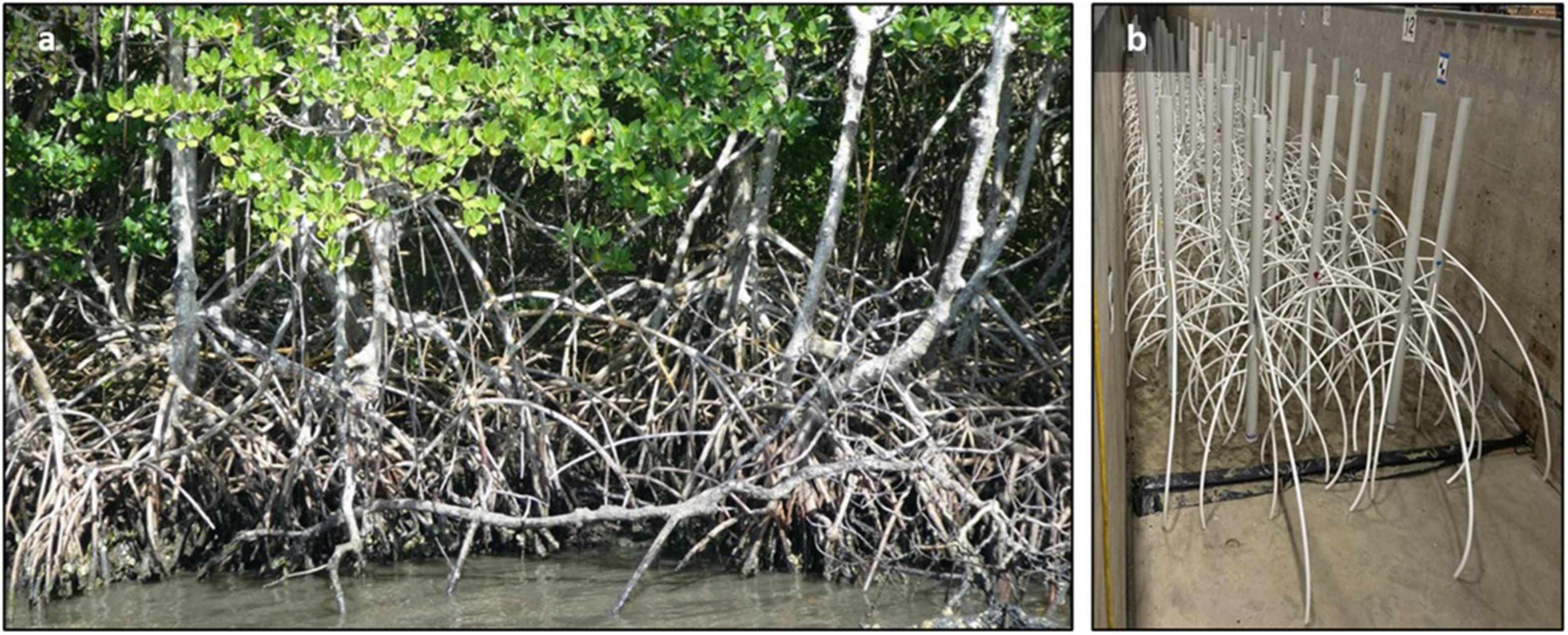
Figure 1. (a) Intertwined trunk-prop root system of R. mangle in St. Lucie Inlet State Park, FL. (b) Physical model of Rhizophora sp. trunk-prop root system.

Physical Model Setup

Mangrove Specimen

The mimics were designed based on previous field measurements of Rhizophora mangle and other mangrove species at sites in Florida (Jimenez et al., 1985; Dawes et al., 1999; Novitzky, 2010) and the Caribbean (Jimenez et al., 1985; Loría-Naranjo et al., 2014). Reported diameters at breast height D_BH ranged from 0.056 to 0.176 m, with a maximum D_BH of approximately 0.10 m at many sites. Reported forest densities ranged from 0.112 to 2.02 stems/m² (Jimenez et al., 1985; Dawes et al., 1999; Novitzky, 2010; Loría-Naranjo et al., 2014). These reported parameters are similar to those reported for Rhizophora sp. sites in India (Danielsen et al., 2005), Vietnam (Bao, 2011), and Malaysia (Ong et al., 1995), although unique sites exhibit variability in both D_BH and stem density. For the present study, a nominal value of D_BH = 0.1 m and two tree densities, 0.75 trees/m² and 0.375 trees/m² were selected to model a mature mangrove forest.

Methods have been proposed to parameterize emergent vegetation including wetland plants (Feagin et al., 2011; Liu et al., 2021; Niazi et al., 2021) and specifically the trunk-prop root system of the Rhizophora genus (Ohira et al., 2013; Niazi et al., 2021). The model of Ohira et al. (2013) was used as the basis of the design of the idealized mangrove tree for this study because it was the basis of previous laboratory studies (Maza et al., 2017, 2019; Tomiczek et al., 2020b) and an ongoing study at another laboratory (Tomiczek et al., 2021) and would facilitate comparisons of the results. Commercially available polyvinyl chloride (PVC) pipe with an outside diameter of 0.1143 m was used for the trunk, resulting in D_BH = 0.1143 m. Following Ohira et al. (2013) yielded a representative model tree with 14 roots and a mean root diameter, D_Root, of 0.0286 m with the tallest root, H_Rmax, located 1.35 m from the ground. The maximum horizontal extent of the tallest root, X_Rmax, was 2.10 m from the base of the model tree. This parameterization was modified for constructability (Tomiczek et al., 2020b), with seven root pairs (i.e., duplicate roots on either side of the tree); the vertical position above ground, H_Ri, maximum root spreading distance, X_Ri, and orientation, θ, (relative to the lowest root pair) for each root are listed in Appendix Table A1. Commercially available cross-linked polyethylene (PEX) with an outside diameter of 0.0286 m was used for the prop roots (Figure 1b).

Bathymetry, Instrumentation, and Test Configurations

The mangrove specimens were installed in the 104 m long × 3.66 m wide Large Wave Flume (LWF) at Oregon State University (OSU) as shown in Figure 2. A piston-type wavemaker was located at the far end of the flume for wave generation. An 18 m long constant-depth section was followed by a piecewise continuous, impermeable bathymetry constructed using 3.6 m by 3.6 m concrete slabs at predetermined locations (termed “bays”) numbered 1–22 in Figure 2. The bathymetry started with a 7 m long 1:12 slope, led to a second 35 m long constant-depth section, and ended with a second 1:12 slope for energy dissipation. The 18 m long mangrove forest was placed on the second constant depth section, set back 11 m from the crest of the first 1:12 slope to minimize effects of wave transformation to the test section.

FIGURE 2

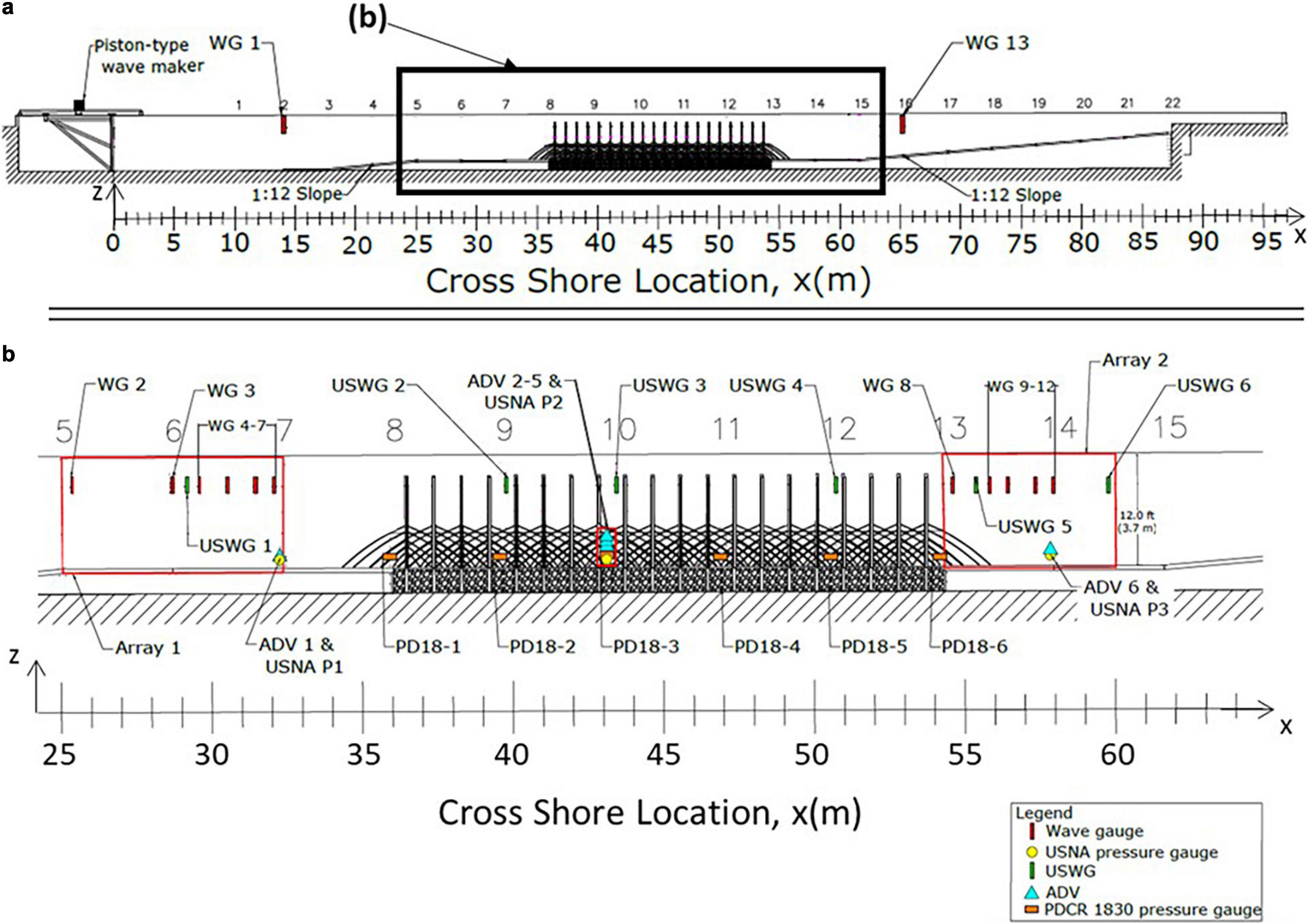
Figure 2. (a) Profile view of flume showing bathymetry, location of mangrove forest, and numbered bays 1–22. (b) Detail profile view of horizontal test section between bays 5–15 showing instrumentation locations in test section.

Figures 2a,b show the locations of instrumentation used during experiments. The seaward-most wave gage (WG1) was positioned at the onset of the foreshore slope, and the landward-most wave gage (WG13) was positioned near the start of the beach to record wave conditions before and after propagating through the test section. Within the forest test section (Figure 2b), a total of 13 wire-resistance wave gages (WG), 6 PDCR 1830 pressure gages (PD18), 6 ultrasonic wave gages (USWG), 3 RBR solo3D pressure loggers, and 6 acoustic-Doppler velocimeters (ADV) were installed to measure hydrodynamic conditions in front of, within, and leeward of the mangrove forest. All WGs, PD18s, USWGs, and ADVs were synchronized to the start of the wavemaker displacement time series and sampled at a rate of 100 Hz. Measured water levels by PD18s were corrected to the free surface accounting for dynamic wave pressure attenuation with depth.

Figure 3a shows a plan view of the LWF. Three configurations were tested for this study: a baseline configuration (BL) with no mangroves to determine the wave attenuation due to bottom and sidewalls and two configurations with a high-density (HD, 0.75 stems/m², Figure 3b) and low-density (LD, 0.375 stems/m², Figure 3c) mangrove forest. When installing the trees (Figure 4a), roots of mangrove specimens that were positioned in locations where their horizontal spreading would intersect the flume walls were precut to account for the flume walls. The model trees were then secured to bases in the test section. A 0.076 m thick concrete cap was used to secure the root ends of the model trees.

FIGURE 3

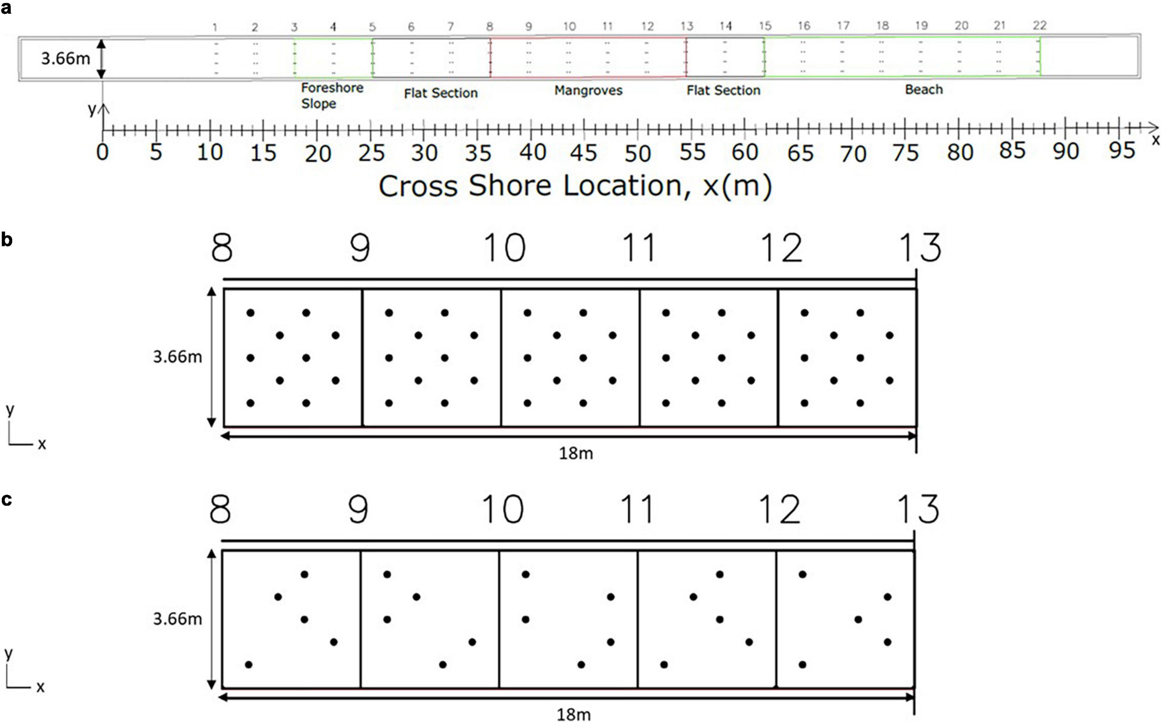
Figure 3. (a) Plan view of large wave flume showing baseline (BL) configuration. (b,c) Detailed view of mangrove test section showing mangrove locations in (b) high-density (HD) and (c) low-density (LD) configurations.

FIGURE 4

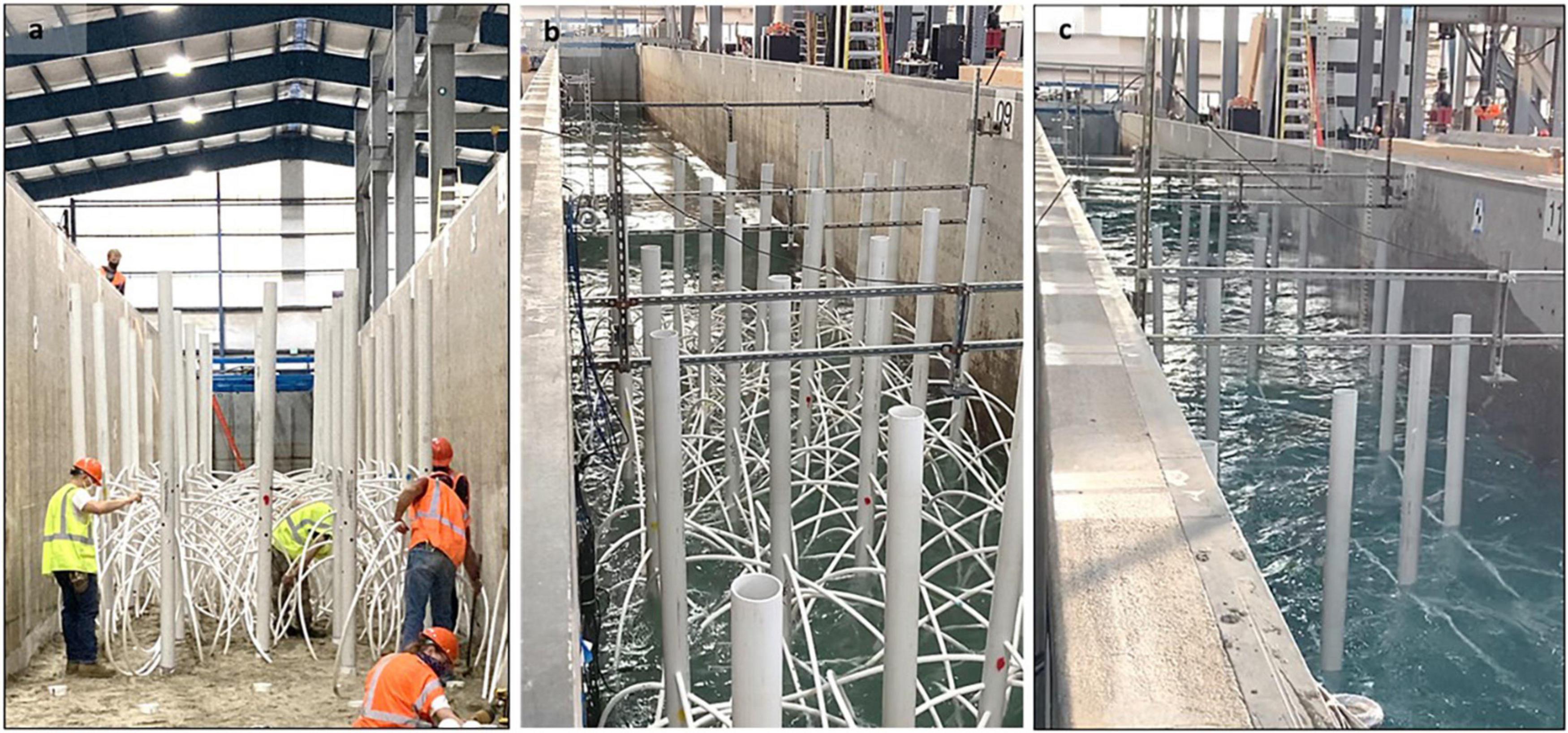
Figure 4. (a) Construction of the model mangrove test section, high-density (HD) configuration; view toward wavemaker with (b) high-density (HD) mangrove configuration, h_v = 0.73 m, H_mo = 0.19 m, T_p = 4.82 s, and (c) low-density (LD) mangrove configuration, h_v = 1.85 m, H_mo = 0.73 m, T_p = 7.45 s.

As seen in Figure 3b, the specimens were positioned in a staggered arrangement for the HD configuration, similar to many previous laboratory studies that used artificial vegetation. By nature of the construction, mangrove specimens were removed from the HD configuration to create the LD configuration. To avoid introducing circulation or cross-mode effects into the model owing to positioning of the specimens, mangroves were selected for removal such that the number of specimens in each 3.66 m by 3.66 m section was reduced from 10 to 5 and such that each cross-shore row (spaced regularly in the alongshore-direction) had a total of 5 trees. This procedure resulted in a non-uniform positioning of specimens for the LD configuration. While forces on individual stems can vary from uniform to random arrangements, idealized and random arrangements have been shown numerically to produce comparable results for overall wave height attenuation (Maza et al., 2015).

Hydrodynamic Conditions

Random and regular waves were generated for the HD, LD, and BL configurations to assess wave attenuation and load reduction by the model mangrove forest (Kelty et al., 2021). Photographs of the HD configuration construction and waves interacting with the HD and LD configurations are shown in Figures 4a–c, respectively. Table 1 lists the wave conditions measured at the seaward-most pressure gage in the mangrove forest section (PD18-1), including water depth at the vegetation h_v, significant wave height H_m0, peak period T_p and wavelength L_p calculated using the peak period. Wave conditions were selected such that three non-dimensional cases of relative wave height H_mo/h_v and relative water depth k_ph_v were considered for random waves and six non-dimensional cases of relative wave height H/h_v and relative water depth kh were considered for regular waves across varying water depths, wave periods, and wave heights. For random waves, dimensionless ratios of water depth at the vegetation to wavelength (h_v/L_p), significant wave height to water depth (H_m0/h_v), vegetation cross-shore length, L_veg, to wavelength (L_veg/L_p) and wavelength to flume width, W, (L_p/W) are also presented in Table 1. Hydrodynamic conditions for regular wave cases are listed in Appendix Table A2.

TABLE 1

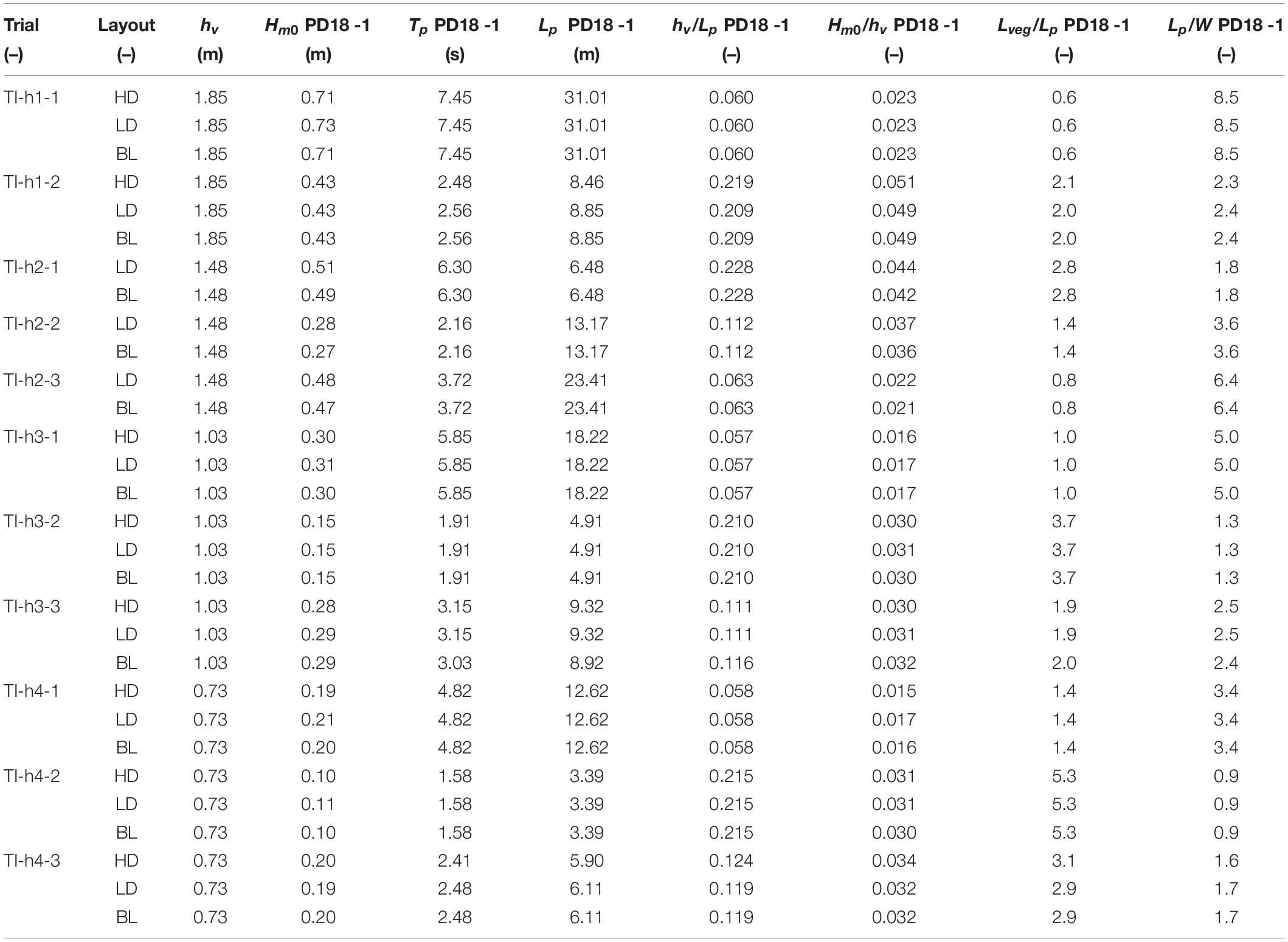
Table 1. Measured wave conditions at test section for random wave trials.

A range of wave conditions were run initially at three water depths at the vegetation test section (h_v = 1.85 m, 1.03 m, 0.73 m) for the HD, LD, and BL configurations. A fourth water depth (h_v = 1.48 m) was added for the LD and BL configurations because of additional availability of the facility, but it was not possible to repeat the HD configuration at h_v = 1.48 m. In general, the significant wave height, H_m0, and peak period, T_p, were chosen for a given water depth h_v to correspond to non-dimensional values of H_m0/h_v = 0.18 or 0.36 and h_v/L_p = 0.06 or 0.11 or 0.22. The purpose was to choose large waves so that the wave decay could be measured accurately, but not so large to avoid depth-limited and steepness-limited wave breaking, ensuring that the primary dissipation mechanisms were due to the wave interaction with the mangroves and due to the side wall and bottom friction. For each trial, 300 individual waves were generated using a JONSWAP spectrum with γ = 3.3.

Projected Area

The total projected area in the direction of flow is essential to estimating the drag coefficient via the Dalrymple et al. (1984) and Mendez and Losada (2004) formulations. For simple geometries such as vertical rods, the estimation is relatively straightforward. However, estimating the projected area of the complex aerial root structures associated with Rhizophora sp. is more involved. Previous studies have utilized photogrammetry in the field (Zhang et al., 2015) and laboratory (Maza et al., 2017, 2019), or 3D laser scanning (Chang et al., 2019) to derive the projected area of a single tree specimen. For fringing mangrove forests, roots of neighboring trees may overlap, creating a dense network (Figure 1). The intertwined root system alters the projected area seen per tree and thus calls for a practical methodology that can extract the projected area of these complex root systems, yet allow for comparison on a per-tree basis.

The HD and LD forests were scanned using a LiDAR system (BLK 360, Leica-Geosystems). The time-of-flight unit used a range 1 laser with a wavelength of 830 nm, and had a 360° and 300° field of view in the horizontal and vertical, respectively. The scanner was equipped with a 15 Mpixel 3-camera system and a 150 Mpixel full-dome capture for high dynamic range (HDR) and light emitting diode (LED) flash calibrated spherical images. For both configurations, seven overhead scans of the forest were taken, with the LiDAR scanner mounted above the test section. Scans were performed at the midpoint of bays numbered 7 – 14 (see Figure 2a). Figure 5 shows an example of the process for scanning the forest and analyzing the LiDAR images for the HD configuration.

FIGURE 5

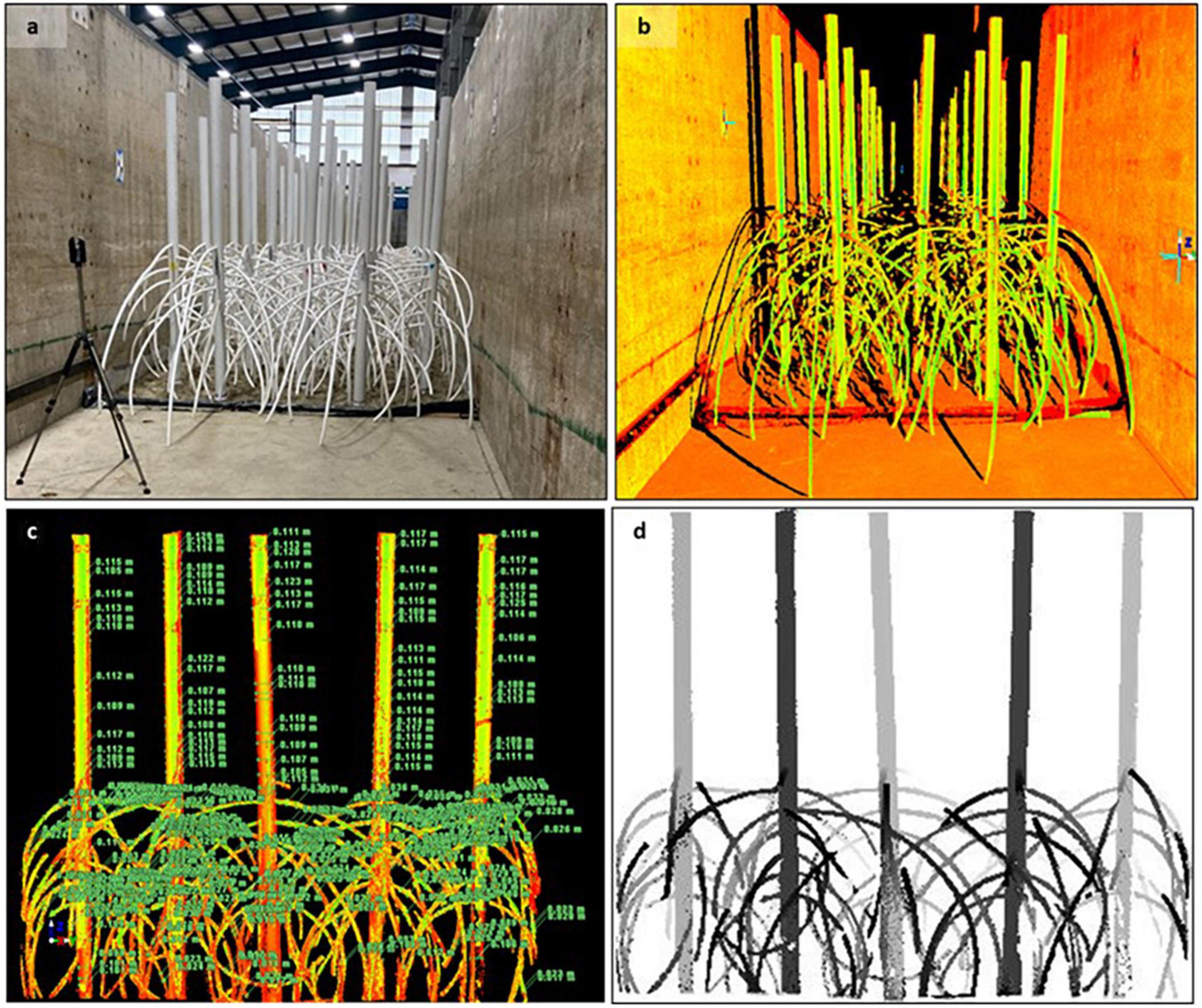
Figure 5. (a) Head-on photograph of HD model forest. (b) Scanned LiDAR image. (c) Extracted stencil showing measurements of trunk and prop roots. (d) Pixelated image for calculating projected area per unit height.

The HD and LD model forest LiDAR scans (Figure 5b) were transferred from the LiDAR scanner and registered using a proprietary software (Cyclone, Leica-Geosystems) to relate multiple scans on a common coordinate system. An alongshore Y-Z cut plane was established at the seaward boundary of the forest section. For the LD configuration, a stencil of 2.0 m cross-shore width (repeating pattern of trees) was identified within the forest to comprise two rows of model specimens, and seven stencils were extracted from bays 10–13. For the HD configuration, five stencils of 2.0 m cross-shore width were extracted from bays 10–13, which were then split into ten half stencils of 1.0 m cross-shore width to minimize under-prediction of the projected area due to root overlap. Extracted stencils and half stencils were manually cleaned for scatter and drift points. Manual measurements of the trunk and root diameters of the first extracted HD stencil (Figure 5c) were taken and compared to the known values of D_BH = 0.1143 m and D_Root = 0.0286 m. The LiDAR measurements underestimated the trunk and root diameter by 2 and 10%, respectively.

The cleaned stencils were then rasterized to create a 1 cm × 1 cm pixelated image of the LiDAR cross section (Figure 5d). Image analysis tools (Matlab R2017) were then used to discretize the pixelated image into horizontal slices of 1 cm height. The projected area was calculated by counting the number of pixels in every horizontal slice and multiplying by the dimensions of one cell (1 cm × 1 cm). The projected area per unit height, A, was then determined by dividing the projected area by the height of the horizontal slice. To check for bias in view direction (landward or seaward), a HD half stencil cross-section was rotated 180° around the z-axis. Its projected area per unit height was compared to that of the original cross-section, and the average variance was negligible. Therefore, the analysis method was not impacted by the direction (landward or seaward) that the cross-section was analyzed. An average was taken of the projected area per unit height for all of the HD and LD model forest stencils to create the representative mean profile and quantify uncertainty of the HD or LD model forest projected area. The mean profiles were divided by the mean number of trees in the analyzed cross-sections to allow for the mean projected area per unit height of the HD and LD model forests to be compared on a per tree basis, A_t. On a per-tree basis, the profiles of the HD mean half stencil and the LD mean stencil show good agreement: the HD mean half stencil’s projected area per unit height per tree was, on average, 1.4% smaller than the LD mean stencil for the root section (0 ≤ h_v ≤ 1.35 m), and 1.9% smaller for the trunk section (h_v > 1.35 m). The HD mean half stencil profile was used for further analysis in the study.

Extracting stencils at different cross-shore positions throughout the forest allowed for the determination of the uncertainty associated with the projected area, as shown in Figure 6. Figure 6a shows the mean projected area per unit height per tree for the HD half stencil (blue line, circles), determined by taking the mean projected area of the ten half-stencils of the HD forest. Horizontal lines denote error bars (one standard deviation) for each 1 cm bin. The mean projected area per unit height per tree, $\overline{A_t}$, calculated by integrating the HD mean half stencil curve to each tested water level, is shown as a vertical solid black line with height equal to its respective water depth. As indicated in the figure, at the lowest two water depths (h_v = 0.73 m and h_v = 1.03 m), $\overline{A_t}$ values are similar; as water depth increases above the root structure, $\overline{A_t}$ decreases due to the influence of the trunks. The root section (0 ≤ h_v ≤ 1.35 m) exhibits greater variability in $\overline{A_t}$ for the measured projected area per unit height per tree than the trunk section (h_v > 1.35 m). The standard deviation at each bin was used to calculate a mean standard deviation, $\overline{{\mathrm{\sigma }}_{At}}$, of the mean projected area per unit height per tree, using the same integration routine for the $\overline{A_t}$ values. These parameters were used to calculate the drag coefficient, C_D, and a range of uncertainty around C_D due to the variability of $\overline{A_t}$.

FIGURE 6

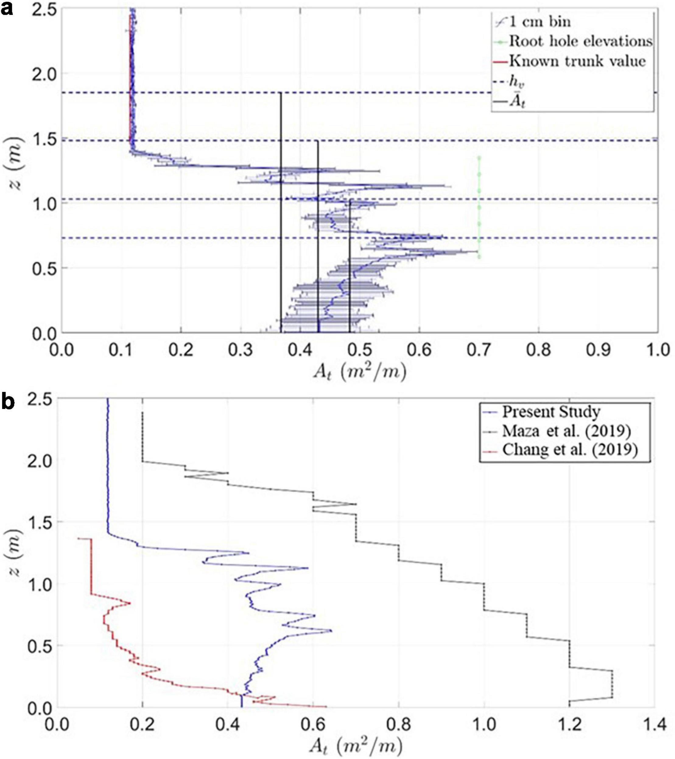
Figure 6. (a) Projected area per unit height per tree, A_t, versus the water depth at the vegetation, h_v, for the high-density (HD) mean half stencil. Error bars represent one standard deviation and vertical lines show mean projected area per unit height per tree, $\overline{A_t}$. (b) Comparison of the projected area per unit height per tree, A_t, for high-density (HD) mean half stencil (blue line and markers), prototype-scale Maza et al. (2019) (black line and markers), and prototype-scale Chang et al. (2019) (red line and markers) model tree profiles. Note change in x-axis scale from (a) to (b).

The HD mean half stencil profile of the projected area per unit height per tree, A_t, was compared with those of the studies by Chang et al. (2019) and Maza et al. (2019) in Figure 6b, rescaling the model trees considered in each study to full-scale. Figure 6b shows elevation z on the y-axis and the projected area per unit height per tree, A_t, on the x-axis, with the prototype-scale specimens of the present study, Chang et al. (2019) and Maza et al. (2019) represented by blue, black, and red lines and markers, respectively. As seen in the figure, differences are observed between the specimens, because each study considered a model tree with a different root structure, trunk diameter, and thus overall projected area per unit height per tree, reflective of the natural variability in real-world Rhizophora systems. The present study shows a reduction in A_t at lower elevations, while the models of Chang et al. (2019) and Maza et al. (2019) consistently increase toward the base of the specimen. This difference may be owing to root overlap in the analyzed stencils causing underestimation of the per-tree projected area per unit height. The present study’s projected area per unit height per tree was generally between those of Chang et al. (2019) and Maza et al. (2019). However, the authors note that the comparison shown in Figure 6b is for the projected area per unit height on a per-tree basis. The three studies considered a range of stem densities during test conditions, which affected the overall blockage provided by the mangrove models.

In the constructed Rhizophora model, the trunk diameter is an order of magnitude larger than the root diameter. That difference affects how fluid flows around either the trunks or the roots, characterized by parameters such as the Reynolds number, Re and Keulegan–Carpenter number, KC. The effective diameter, D_e can be used to characterize the flow around the model trees by taking a weighted average of the trunk and root diameters. The effective diameter was calculated at each water level as

$$D_e=\frac{\overline{A_t}}{(1+\overline{n_R})}(4)$$

where $\overline{n_R}$ is the mean number of roots at each tested water level, determined though visual analysis. Table 2 presents the mean projected area per unit height per tree, standard deviation of mean projected area per unit height per tree, mean number of roots, and effective diameter for each water depth at the vegetation tested. In general, D_e values were consistent, ranging from 0.034 m at the lowest water level to 0.041 m at the highest water level.

TABLE 2

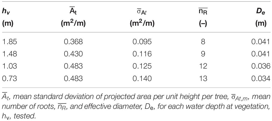
Table 2. Mean projected area per unit height per tree.

Wave Attenuation Rates and Drag Coefficients for Random Wave Trials

Wave Attenuation Rates

The wave gage arrays positioned at Array 1 (seaward) and Array 2 (inland) of the mangrove forest (Figure 2b) were used to analyze the incident spectral estimate of the significant wave height, H_m0,i, and the reflected spectral estimate of the significant wave height, H_m0, using the methods proposed by Zelt and Skjelbreia (1993) and Gronbech et al. (1997). The total (incident plus reflected) spectral estimate of the significant wave height, H_m0, was used for the WGs and PD18s in the test section. An example of the cross-shore variation of H_m0 with respect to the neutral position of the wavemaker (x = 0 m) is shown in Figure 7 for WGs (blue circles) and PD18s (green diamonds) for wave case TI-h3-3, with h_v = 1.03 m, H_m0 = 0.310 m, and T_p = 3.10 s for the HD (dark colors), LD (intermediate colors), and BL (light colors) configurations. The incident (triangles) and reflected (squares) wave heights at WG arrays seaward and inland of the mangrove forest are also shown. At Array 2, the wave reflection from the 1:12 impermeable slope was estimated to be in the range 0.02 < H_m0 < 0.03 m with an average reflection coefficient of 18% and standard deviation of 4%, which is close to the limits of this methodology. At Array 1, the reflected wave was slightly higher with an average reflection of 22% and standard deviation of 7%. This larger value could be due to reflection from the mangrove forest.

FIGURE 7

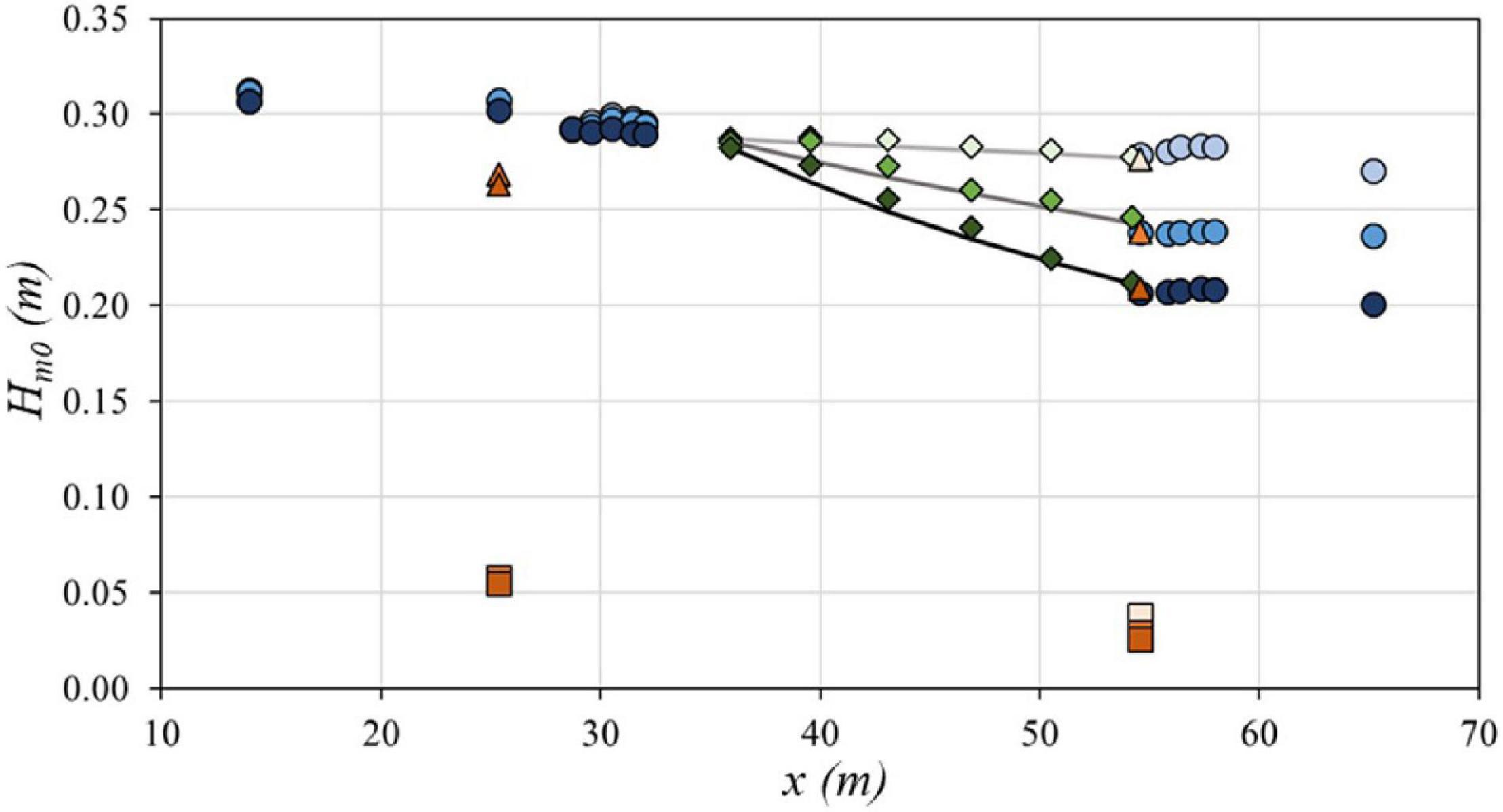
Figure 7. Total spectral estimate of the significant wave height with respect to x-location for WGs (blue circles) and PD18s (green diamonds) and the incident spectral estimate of the significant wave height (orange triangles), and reflected spectral estimate of the significant wave height (orange squares) for the high-density (dark colors), low-density (intermediate colors), and baseline (light colors) configurations for random wave case TI-h3-3, h_v = 1.03 m, H_m0 = 0.310 m, T_p = 3.10 s.

The H_m0 values from the pressure gages located in the start and end of the mangrove forest (PD18-1 and PD18-6) were similar to the mean H_m0 values from Array 1 and 2, respectively. Therefore, the H_m0 values from the pressure gages in the mangrove forest (PD18-1 to PD18-6, 35.9 m < x < 54.2 m) were used to fit wave height decay curves (solid line in Figure 7) for each case using Equation (1), using the least squares method and setting the y-intercept to the value of H_m0 at PD18-1, returning a value of the decay rate, $\tilde{\mathrm{\alpha }}$. For all layouts, H_m0 decreased landward and decay rate $\tilde{\mathrm{\alpha }}$ increased with forest density.

As seen in Figure 7, there was measurable wave height attenuation due to side wall and bottom friction in the baseline case. Therefore, the wave attenuation due to the mangrove forest, ${\tilde{\mathrm{\alpha }}}_m$, was calculated by subtracting $\tilde{\mathrm{\alpha }}$ of the BL configuration from those of the HD and LD configurations. Figure 8 shows ${\tilde{\mathrm{\alpha }}}_m$ versus h_v for the HD (dark blue circles) and LD (intermediate blue circles) configurations for random wave trials. For both the HD and LD configurations, ${\tilde{\mathrm{\alpha }}}_m$ is greatest at the shallowest water depths, where the mean projected area per unit height, $\overline{A_t},$ was the largest. The ${\tilde{\mathrm{\alpha }}}_m$ coefficient decreases approximately linearly as water depth increases. The figure shows that ${\tilde{\mathrm{\alpha }}}_m$ does not vary significantly between the different non-dimensional wave cases for each water depth, suggesting that ${\tilde{\mathrm{\alpha }}}_m$ is predominantly dependent on the water depth at the vegetation, and subsequently, the mean projected area per unit height influencing the fluid flow. The average ratio of the ${\tilde{\mathrm{\alpha }}}_m$ coefficients for the HD to LD configurations for a given water depth and wave condition was 2.0 for random waves, with a standard deviation of 0.12. This ratio is the same as the HD/LD forest density ratio of the mangrove forests, suggesting a linear relationship between the decay rate and forest density, similar to the relationship between the wave height decay coefficient and stem density was found for emergent vegetation by Anderson and Smith (2014).

FIGURE 8

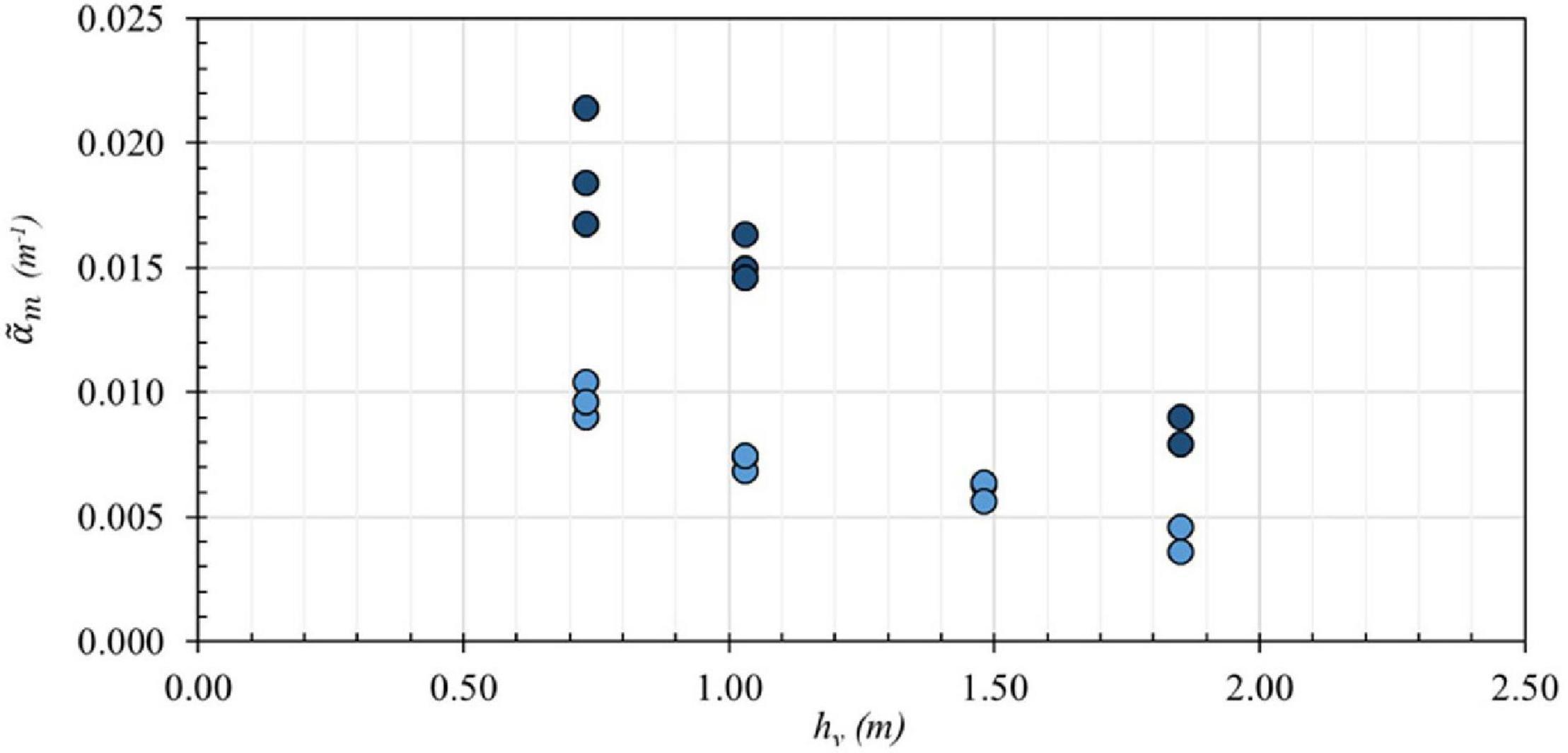
Figure 8. Wave height decay coefficient, ${\tilde{\mathrm{\alpha }}}_m$ versus the water depth at the vegetation, h_v, for random wave cases for the high-density (HD) (dark blue circles) and low-density (LD) (intermediate blue circles) configurations.

The uncertainty in the decay rate, ${\mathrm{\sigma }}_{{\tilde{\mathrm{\alpha }}}_m},$was characterized based on the difference between measured wave heights and predicted values from the best-fit curves for each wave case and layout. This uncertainty did not include potential bias in estimating H_m0 from the pressure transducers from linear wave theory. Table 3 lists ${\tilde{\mathrm{\alpha }}}_m$, ${\mathrm{\sigma }}_{{\tilde{\mathrm{\alpha }}}_m},$ and the average HD to LD ${\tilde{\mathrm{\alpha }}}_m$ coefficient ratio for each random wave case, with hydrodynamic conditions reported at the seaward-most pressure gage (PD18-1). Corresponding values for regular waves were similarly determined and are presented in Appendix Table A2.

TABLE 3

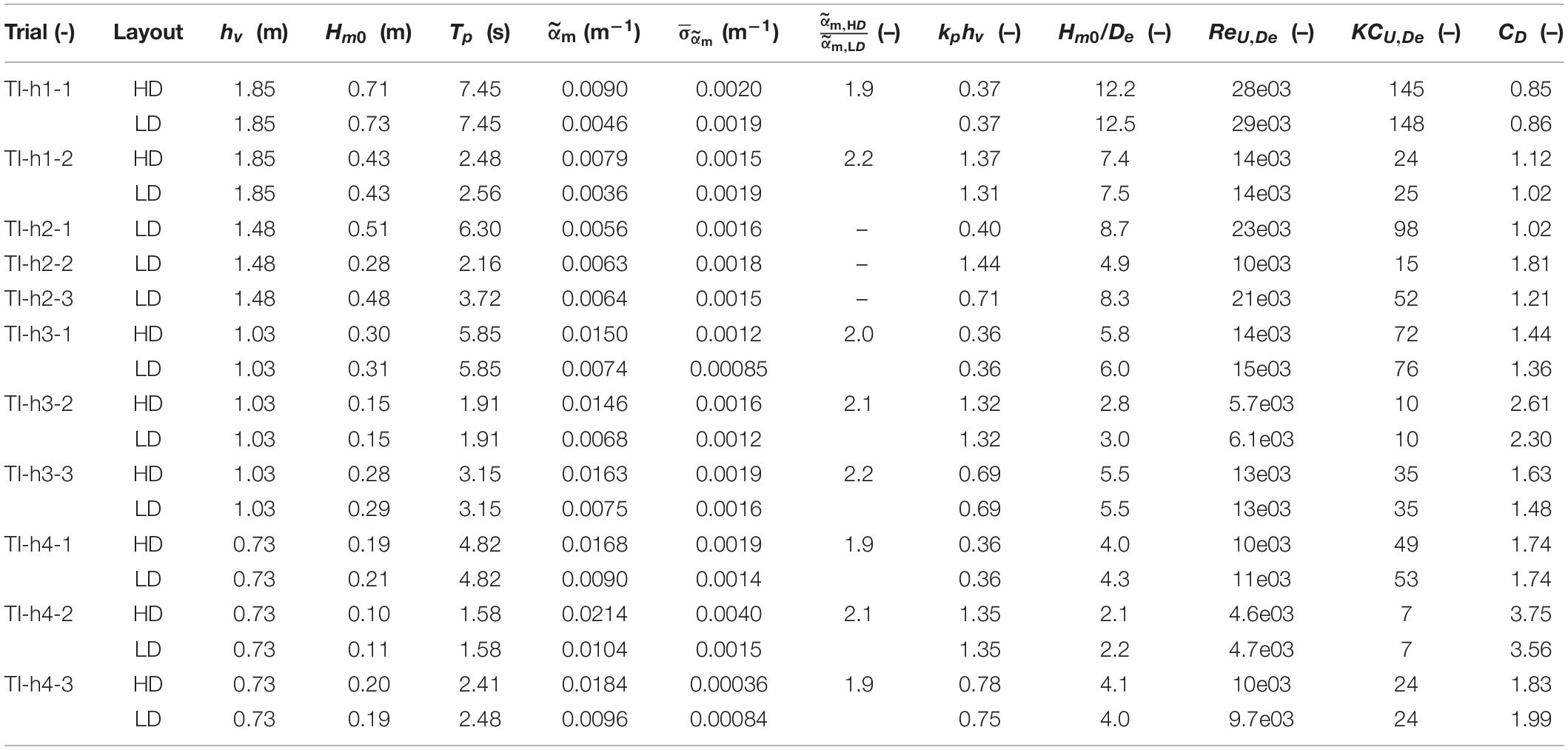
Table 3. Measured H_m0 and T_p values at PD18-1, ${\tilde{\mathrm{\alpha }}}_m$, HD/LD ratio of the ${\tilde{\mathrm{\alpha }}}_m$ coefficient, k_ph_v, H_m0/D_e, Re_U,De, KC_U,De, and C_D values for random wave cases.

Drag Coefficients

The drag coefficient, C_D, for each wave case and configuration was calculated using ${\tilde{\mathrm{\alpha }}}_m$ and Equation (3). The C_D values were then related to the Reynolds number, Re_U,De, calculated using the depth-averaged velocity, U, and the effective diameter, D_e. Table 3 further lists C_D values for each random wave case with hydrodynamic conditions given at PD18-1 for the HD and LD layouts, as well as Re_U,De and the Keulegan–Carpenter number, KC_U,De, determined using the depth-averaged velocity and effective diameter, while Appendix Table A2 provides corresponding values for regular waves, where Equation (2) was used to calculate C_D values. While for most trials KC_U,De was large, indicating drag dominance, a few cases were identified with KC_U,De ≤ 15, where the inertial force contributions are expected to be significant.

Relationships between the calculated drag coefficient and the Reynolds number were investigated for random and regular wave conditions as shown in Figure 9. Figure 9a shows C_D versus Re_U,De on a linear scale for the HD (squares) and LD (triangles) configurations for random wave conditions. Colors indicate the three tested ranges of relative water depth, k_ph_v, for random waves: 0.30 < k_ph_v < 0.40 (dark red), 0.70 < k_ph_v < 0.80 (intermediate red), and 1.30 < k_ph_v < 1.45 (light red). As seen in Figure 9a, C_D values show a consistent dependence on Reynolds number for the forest densities and relative water depth ranges considered in these experiments. Lower C_D values are observed for higher Reynolds numbers and lower relative water depths. Cases with larger C_D values correspond with cases that indicated inertial force predominance. The minimum C_D value observed in this study for random waves was 0.85, occurring at the second largest Re_U,De value and smallest k_ph_v range, and the largest observed C_D value was 3.75, corresponding to the lowest Re_U,De value and largest k_ph_v range. Figure 9b shows C_D versus Re_U,De on a linear scale for the HD (squares) and LD (triangles) configurations for regular wave conditions, with colors indicating tested ranges of relative water depth, kh_v: 0.30 < kh_v < 0.45 (dark orange), 0.45 < kh_v < 0.80 (intermediate orange), and 1.10 < kh_v < 1.40 (light orange). C_D values for regular waves varied from 0.37 to 1.74 for the range of Re_U,De tested and in general showed agreement with C_D values for random waves for similar Reynolds numbers.

FIGURE 9

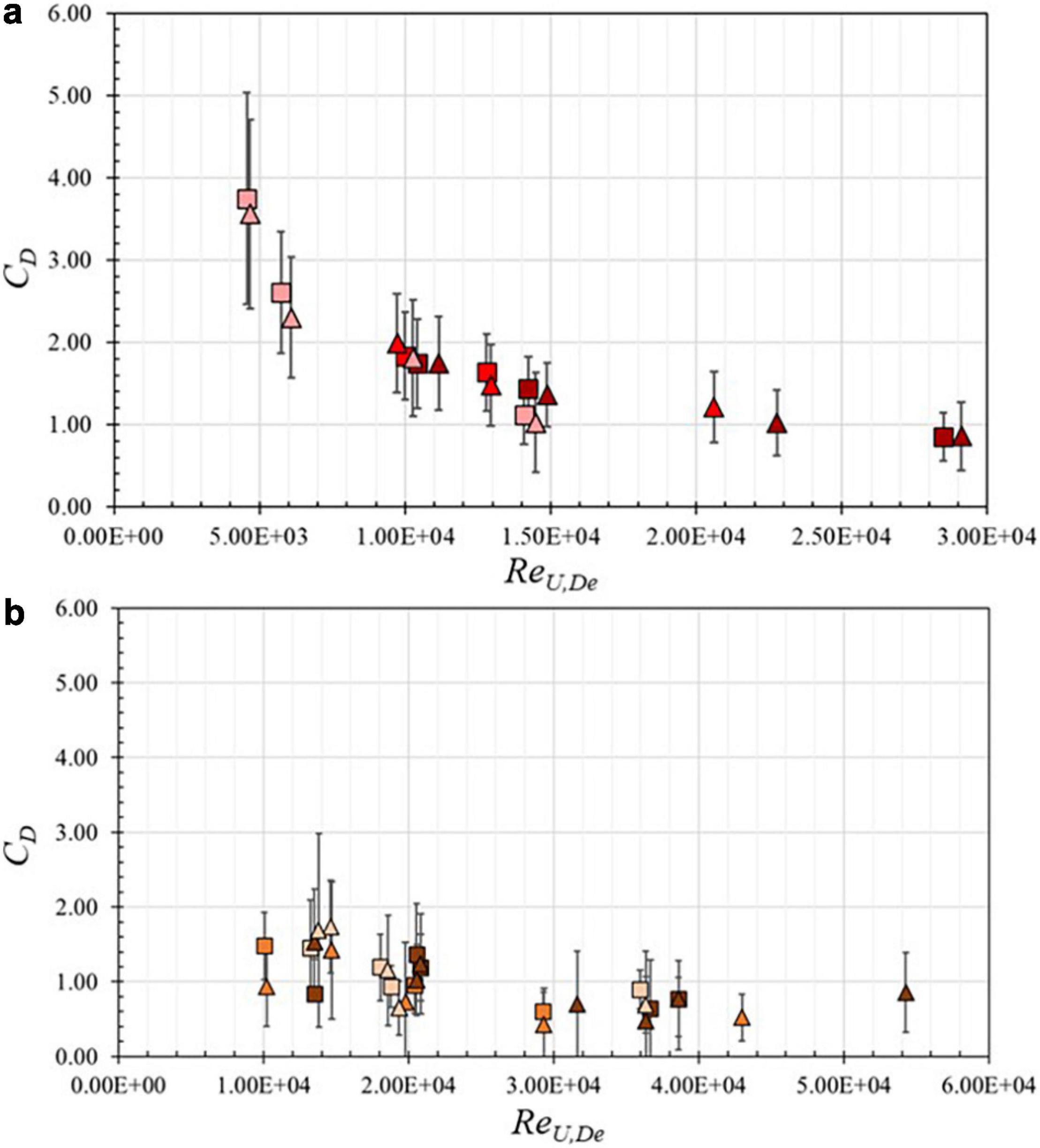
Figure 9. Drag coefficient, C_D, versus the Reynolds number, Re_U,De on a linear scale for high-density (squares) and low-density (triangles) configurations designated by relative water depth. (a) Random wave cases, 0.30 < k_ph_v < 0.40 (dark red), 0.70 < k_ph_v < 0.80 (intermediate red), and 1.30 < k_ph_v < 1.45 (light red). (b) Regular wave cases, 0.30 < kh_v < 0.45 (dark orange), 0.45 < kh_v < 0.80 (intermediate orange), and 1.10 < kh_v < 1.40 (light orange). Vertical bars show combined uncertainty due to $\overline{A_t}$ and ${\tilde{\mathrm{\alpha }}}_m.$ Note change in x-axis scale from (a) to (b).

The combined uncertainty, σ_CD, due to estimates of the projected area per unit height, $\overline{A_t}$, and measured decay rate, ${\tilde{\mathrm{\alpha }}}_m$, was determined by:

$$\frac{{\mathrm{\sigma }}_{C_D}}{C_D}={\left[{\left(\frac{\overline{{\mathrm{\sigma }}_{A_t}}}{\overline{A_t}}\right)}^2+{\left(\frac{\overline{{\mathrm{\sigma }}_{{\tilde{\mathrm{\alpha }}}_m}}}{{\tilde{\mathrm{\alpha }}}_m}\right)}^2\right]}^{\frac{1}{2}}(5)$$

where $\overline{{\mathrm{\sigma }}_{At}}$ and $\overline{{\mathrm{\sigma }}_{\tilde{\mathrm{\alpha }}m}}$ are the estimated uncertainties in the projected area and decay rate, respectively (Table 3 and Appendix Table A2), and are shown as vertical bars in Figures 9a,b. In general, uncertainty in C_D increases slightly as the Reynolds number decreases. The overall mean value of the uncertainty is $\overline{{\mathrm{\sigma }}_{CD}}$ was 0.58 and 0.56 for random and regular waves, respectively.

Scaling Law for Comparison With Reduced-Scale Data and Design Equation for C_D

The data from the present study were compared to data from the 1:6- and 1:7- reduced-scale experiments of Chang et al. (2019) and Maza et al. (2019), respectively. Maza et al. (2019) considered regular and random waves, and Chang et al. (2019) considered regular waves. Both Chang et al. (2019) and Maza et al. (2019) reported drag coefficients as a function of the Reynolds number. Maza et al. (2019) determined Re based on the projected area per unit width, and thus had larger overall values of Re than if the characteristic length scale had been taken as the diameter of the trunk or root as is more common in studies of emergent vegetation. Chang et al. (2019) used the D_BH as the characteristic length scale to determine Re.

It is well known that Reynolds similitude does not hold in a reduced-scale hydraulic model test when Froude similitude is used for the kinematic scaling. Therefore, to compare the two previous reduced-scale studies with the current prototype-scale study, a scaling relation is proposed for the Reynolds number:

$$R{e}_p=\mathit{\hspace{1em}\hspace{1em}}R{e}_m{\mathrm{\lambda }}^{\frac{3}{2}}(6)$$

where λ is the prototype-to-model geometric scale ratio and Re with subscripts p and m refer to the prototype- and reduced-scale Reynolds numbers, respectively, and the 3/2 results from Froude scaling. Similar scaling of the Reynolds number has also been used in reduced-scale studies focused on permeable core material for rubble mound breakwaters (e.g., Jensen and Klinting, 1983; Martín et al., 2003; Losada et al., 2016), which also relies on turbulence to dissipate wave energy.

Equation (6) was applied to the data of Chang et al. (2019) and Maza et al. (2019) with λ 6 and λ 7, respectively, as shown in Figure 10. As noted earlier, Maza et al. (2019) used the projected area as the characteristic length scale for Re. To provide a consistent basis for comparison, D_BH was used as the characteristic length scale to rescale their reported values of Re. In the figure, drag coefficients from the present study for regular and random wave cases are shown as light red squares and dark red circles, respectively. Drag coefficients reported by Maza et al. (2019) for regular and random wave cases are shown as light green squares and dark green circles, respectively. Drag coefficients reported by Chang et al. (2019) are shown as light blue squares. As seen in the figure, rescaling the Reynolds number results in good agreement across all three studies, despite the differences in the studies’ scales, wave conditions, and model tree geometries, suggesting that the method is fairly robust.

FIGURE 10

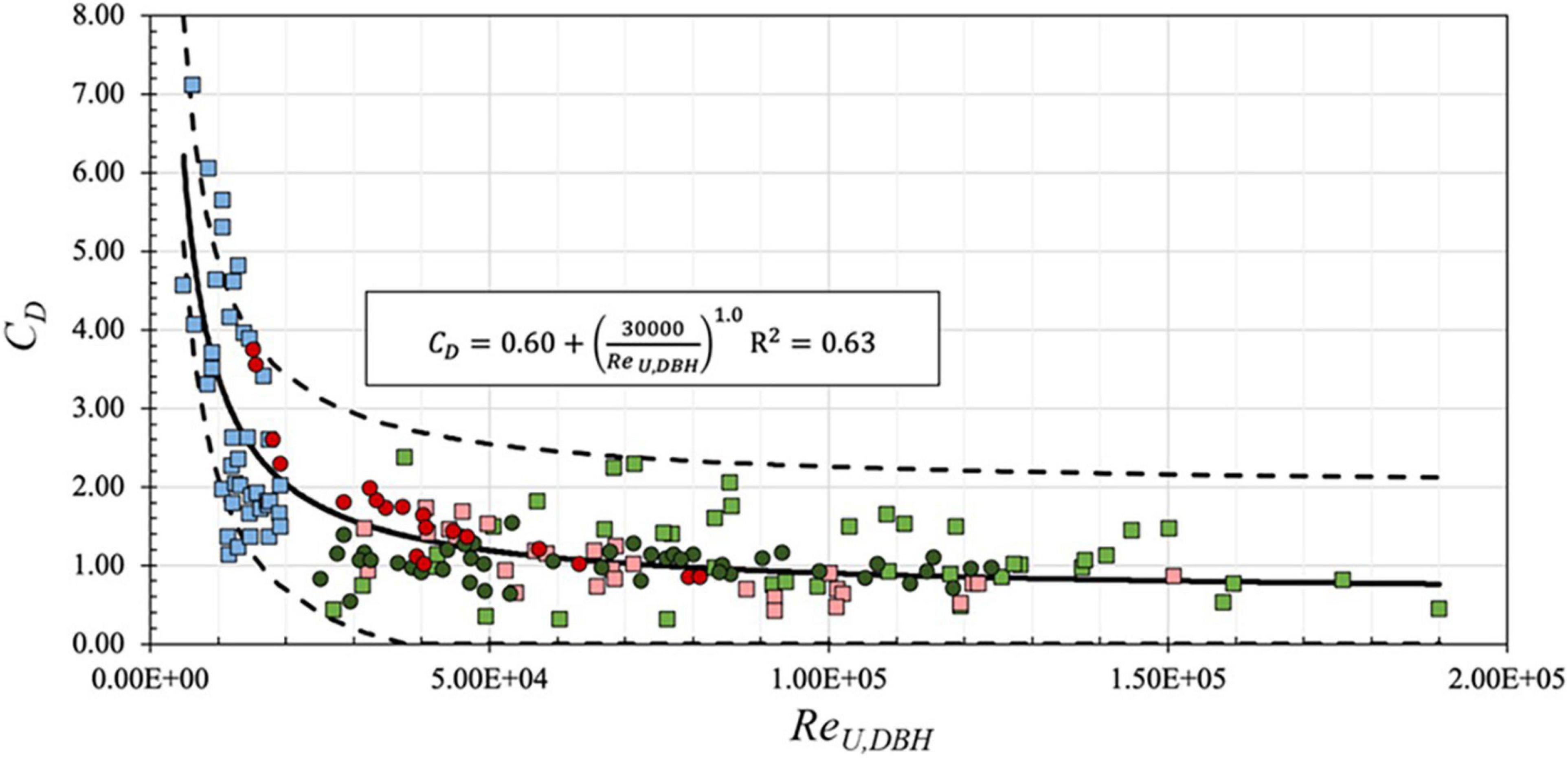
Figure 10. Drag coefficient, C_D, versus the Reynolds number, Re_U,DBH, on a linear scale for data from present study random (dark red circles) and regular (light red squares) waves, Maza et al. (2019) random (dark green circles) and regular (light green squares) waves, and Chang et al. (2019) regular (light blue squares) waves. Solid black line indicates the fitted equation with asymptote value 0.6 [Equation (8)]. Dashed black lines indicate 95% confidence intervals.

A best-fit line using the empirical equation of the form C_D = a₁ + (a₂/Re_U,DBH)^a3 was found for the combined data (Chang et al., 2019; Maza et al., 2019, and present study) with coefficients a₁ = 0.70, a₂ = 26,000, a₃ = 1.0, and R² = 0.63 for the range 4.9e03 < Re_U,DBH < 1.9e05:

$$C_D=0.70+{\left(\frac{26,000}{R{e}_{U,DBH}}\right)}^{1.0}(7)$$

Equation (7) was modified by setting the asymptote value a₁ = 0.60, consistent with results from Sarpkaya and Isaacson (1981), an accepted value for waves on vertical piles, giving an alternative best-fit line with a₂ = 30,000, a₃ = 1.0:

$$C_D=0.60+{\left(\frac{30,000}{R{e}_{U,DBH}}\right)}^{1.0}(8)$$

Equation (8) results in similar estimations of C_D based on Re_U,DBH and is shown as a solid line in Figure 10, with dashed lines showing 95% confidence intervals assuming a normal distribution of the data. As seen in Figure 10, Equation (8) shows good agreement with the combined data, with R² = 0.63. Data are generally within confidence intervals, particularly for higher Reynolds numbers. Equation (8) may therefore be used in engineering design to determine the appropriate drag coefficient for mangroves over the range of hydrodynamic conditions considered here. This drag coefficient may then be used to calculate wave height decay and attenuation via the equations proposed by Mendez and Losada (2004) for random waves.

Comparison With Drag Coefficient Relations for Emergent Vegetation

It is of some interest to show the comparison of the three mangrove studies of Figure 10 with previous studies considering emergent wetland vegetation (e.g., Spartina alterniflora) modeled using rigid cylinders (Hu et al., 2014; Ozeren et al., 2014) or flexible tubing (Anderson and Smith, 2014), since these studies also model C_D as a function of Re in the form of Equation (8). Table 4 lists the vegetation studied, wave conditions, range of Reynolds numbers considered, and proposed equation for the drag coefficient as a function of the Reynolds number for the combined data of this study (Chang et al., 2019; Maza et al., 2019, and present study) and the previous investigations of emergent vegetation.

TABLE 4

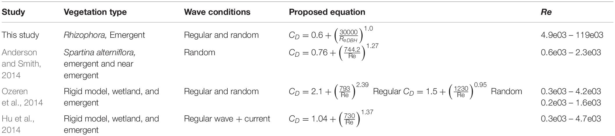
Table 4. Proposed equations for drag coefficient C_D as a function of the Reynolds number, Re.

The equations presented in the studies listed in Table 4 are shown in Figure 11, which shows C_D plotted against Re on a logarithmic scale. The black dash-dot line indicates the best-fit line developed from the combined data focusing on the Rhizophora sp. of this study (red circles) and rescaled data of Chang et al. (2019) (blue circles) and Maza et al. (2019) (green circles). Drag coefficient relations for emergent wetland vegetation are shown as dashed lines for random wave data from Anderson and Smith (2014) (orange), regular wave with current data from Hu et al. (2014) (red), and regular and random wave data from Ozeren et al. (2014) (light and dark blue, respectively). As seen in the figure, the Rhizophora studies report higher Reynolds numbers (under prototype conditions) than the emergent wetland vegetation studies, which is reasonable considering the stem diameters of the emergent wetland vegetation studies were 1–2 orders of magnitude smaller than the D_BH values of the Rhizophora studies. The Rhizophora studies were also tested under larger wave conditions than the emergent vegetation studies. The three emergent vegetation studies show a fair amount of variability in C_D. Had the results of Chang et al. (2019) and Maza et al. (2019) not been rescaled, these data would have appeared among the dashed lines of Figure 11, and could have been misinterpreted as having good agreement with previous studies of emergent wetland vegetation with smaller characteristic length-scales. However, there is a clear separation between the previous studies of emergent wetland vegetation and the mangrove studies at prototype-scale. This comparison reinforces the necessity of proper consideration of Reynolds-dependent C_D values estimated from reduced-scale tests based on the vegetation archetype considered.

FIGURE 11

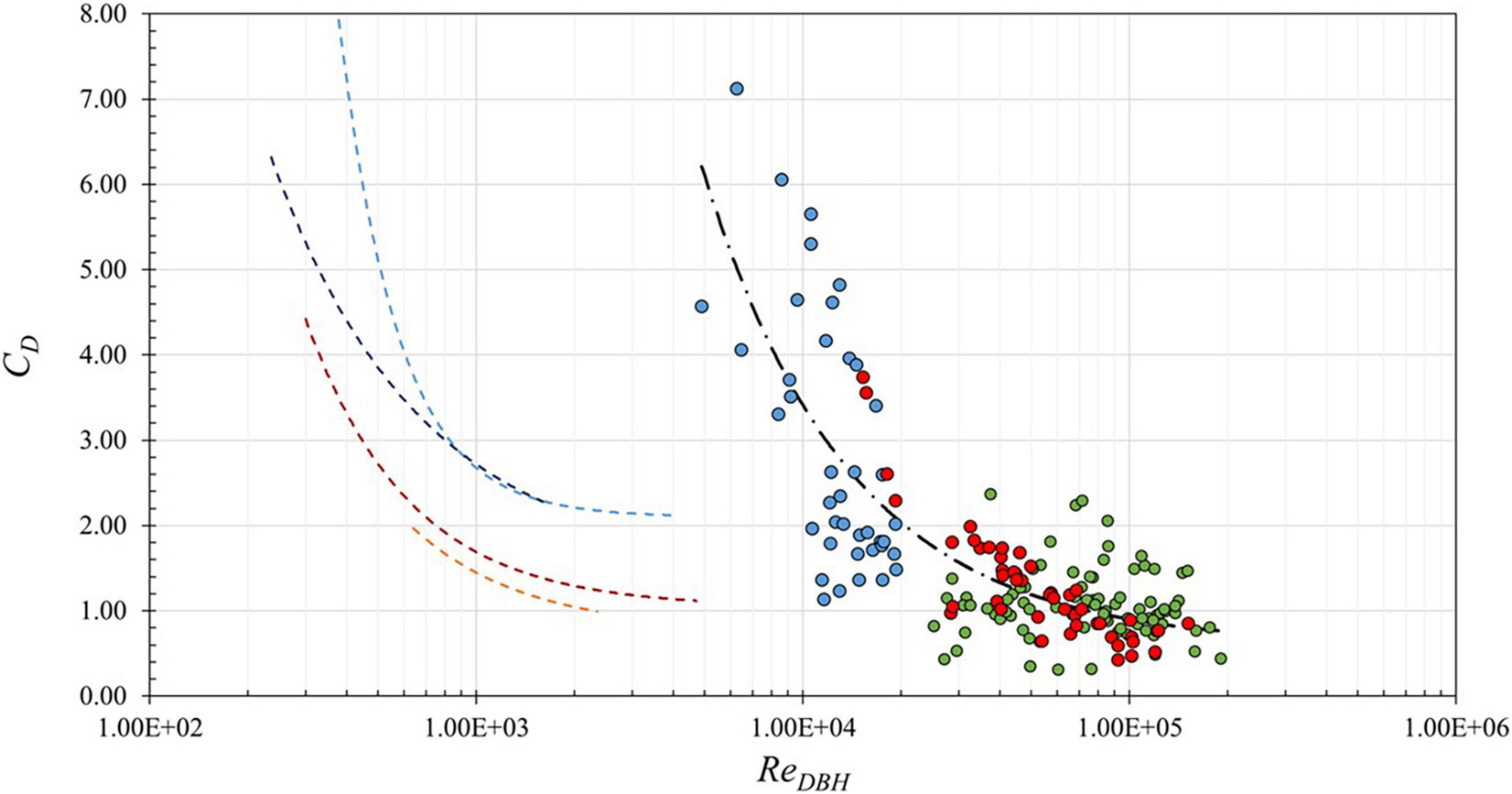
Figure 11. Drag coefficient C_D vs. Reynolds number Re_DBH on logarithmic scale for comparison of previous studies of emergent wetland vegetation (dashed lines): Anderson and Smith (2014) (random waves, orange), Hu et al. (2014) (regular waves + current, red), Ozeren et al. (2014) (regular and random waves, light and dark blue, respectively) to the proposed equations for the combined mangrove data (black dash-dot line) of present study (red circles), Chang et al. (2019) (blue circles), and Maza et al. (2019) (green circles). Note x-axis origin is at 1.00e02.

Discussion

Implications for Shoreline Protection

Results of this study can be used to inform coastal engineers and stakeholders on the potential of leveraging mangroves in engineering with nature projects. The methodology presented here for LiDAR-based characterization of the projected area and effective diameter of the mangrove forest can be extended to field applications to complement conventional methods (i.e., calipers, rulers, and measuring tape) for determining mangrove geometric characteristics. The method further can provide a non-destructive and accurate process for estimating D_BH and D_Root values of complex sites. While previous studies have used terrestrial-based LiDAR to quantify the biomass of mangrove forests (Feliciano et al., 2014; Olagoke et al., 2016) using non-destructive methods, these studies did not report projected area. Therefore, the methodology proposed here may expand upon ecological studies that use terrestrial-based LiDAR scanning for engineering applications to obtain a representative cross-section of the projected area of a mangrove forest for predicting the forest’s effects on wave attenuation. LiDAR measurements taken at different points in time can be used to assess how the projected area changes as a forest matures, after a system is damaged by a storm event (Lagomasino et al., 2021), and throughout the recovery process. The effect of uncertainty in the projected area on the drag coefficient and ultimately hydrodynamic transformation through a mangrove forest can also be quantified. Accurately characterizing the uncertainty of a system’s performance is essential for making conservative design decisions and incorporating redundancy in a shoreline protection project.

Results of this study indicate that even mangrove forests of moderate cross-shore width (∼10–50 m) can provide measurable reduction in wave heights, building on previous studies that have considered greater forest expanses (e.g., Maza et al., 2019). For random waves, wave height reductions of 13–28% and 6–16% were observed over the 18 m cross-shore forest distance for the HD and LD configurations, respectively, and for regular waves, wave height reductions of 12–32% and 6–22% were observed for the HD and LD configurations, respectively. The proposed Equation (8), which synthesizes the results of the present prototype-scale tests and two previous reduced-scale tests from the literature, can be used for a specific site given information about the mangrove forest geometry and design hydrodynamic conditions. This study also confirms that a relatively simple scaling relation of the Reynolds number can be used to compare data of reduced-scale tests under Froude similitude. The agreement between the present study’s data collected at prototype scale and the rescaled data of Chang et al. (2019) and Maza et al. (2019) based on Equation (6) supports the use of reduced-scale models, which are often more cost-, time-, and labor- effective, to improve the robustness of C_D vs. Re relationships for investigation of wave attenuation through vegetation, provided that Reynolds number scaling is considered.

Physical Model Considerations

Sources of uncertainty in addition to the two discussed in this study may affect the drag coefficient of Rhizophora sp. trees. The LiDAR methodology presented here may result in increased uncertainty in geometric measurements at field sites owing to challenges with determining the projected area of submerged portions of a mangrove forest or due to blockage by the forest canopy. While the majority of the cases tested fell within the drag-dominated regime, several cases were located within the inertia-dominated regime as indicated by the KC number in Table 3 and Appendix Table A2. These cases correspond to the largest relative water depths tested for the study. The inertial predominance indicated for these cases could lead to higher estimations of the drag coefficient, C_D, from the Mendez and Losada (2004) C_D equation [Equation (3)], which neglects inertial force in the derivation. This study did not collect direct force measurements on the model tree specimens, so the possible C_D overestimation by the Mendez and Losada (2004) equation for these cases could not be fully quantified. In addition, the derived equations came from studies that did not include a canopy for the idealized model tree. The canopy’s added effects, especially at higher water depths and milder wave conditions, could alter the drag coefficients from those presented in this study. Similarly, both the present study and Maza et al. (2019) only considered the primary prop root in constructing the model trees, while Chang et al. (2019) included the primary roots with the secondary and tertiary prop roots branching off of the primary roots. The tertiary and secondary roots provide more projected area and potentially more protection. Therefore, neglecting the canopy and additional prop roots provides conservative estimations of the protection provided by the mangroves for the range of hydrodynamic conditions considered.

In nature, mangrove forests comprise trees of different ages, growth stages, and species. The protection that mangrove forests provide can change depending on biological variables such as forest age, growth, and structure, or damage sustained during an extreme event such as a hurricane or tsunami. To assess the protection provided at various stages of the forest’s lifetime, a weighted average drag coefficient could be calculated if the percentage makeup of the forest for the different diameters at breast height are known. Similarly, natural variation in projected area through the forest may affect wave attenuation, and therefore protocols for assessing the geometric properties at various cross-shore locations within a forest are required. Understanding the temporal and spatial variation of the protection provided by mangroves is essential to quantifying the long-term protection that these forests can provide. In addition to wave height reduction, other performance metrics such as load reduction on sheltered structures or overtopping reduction of inland infrastructure may also be considered for engineering design.

Implementing mangroves and other natural systems at ecologically viable sites is critical to ensure that these systems can mature and provide the desired engineering services. For example, the day-to-day wave climate, hydrologic connectivity, and water quality can affect mangrove growth and vulnerability, and disruptions such as extreme storms, prolonged flooding, and sediment smothering can cause significant die off (Lagomasino et al., 2021). Threshold conditions at which natural systems fail to perform their design engineering service must be identified. Similarly, the ecology of these systems must be considered in engineering design to determine where these nature-based solutions are viable adaptation alternatives and understand what conditions may threaten the survivability of a project. The ability of mangroves to keep up with relative sea level rise at local sites must also be considered (Saintilan et al., 2020). Incorporating gray infrastructure such as rubble mound sills could protect the shoreline and juvenile green infrastructure systems as the vegetation matures; however, best practices for combining green and gray infrastructure must be developed, as well as methods to assess the combined performance of these hybrid systems. The most resilient mangrove system may not necessarily be the same system that optimizes engineering performance, and so a balance between ecological requirements and engineering performance must be achieved. Future research focused on these hybrid systems is needed to fully answer these questions and identify the critical components for successful design.

Conclusion

This paper presents results of an idealized, prototype-scale physical model to quantify protection provided by a Rhizophora sp. mangrove forest of moderate (18 m) cross shore width for use in engineering with nature projects. Results of this study lead to the following six conclusions:

(1) The LiDAR methodology developed for this study accurately characterized the representative projected area per unit height and associated uncertainty of the mangrove forest, allowing for an effective diameter of the system to be determined. Trunk and prop root LiDAR measurements were accurate to within 2 and 10% of known values, respectively.

(2) Mangroves of moderate cross-shore width had a measurable effect on wave attenuation for the range of wave conditions tested here. Wave height decay rates of 0.008–0.021 m^–1 and 0.004–0.010 m^–1 were observed for the high-density and low-density configurations, respectively.

(3) Increasing the density of the mangrove forest by a factor of two increased the wave decay coefficient by a factor of 2.0 on average for the random wave conditions and by 2.2 for regular wave conditions. This result is consistent with similar observations in the literature and suggests that the wave height decay was not affected by gridded or random mangrove layouts, but rather by the density variation, in agreement with the numerical findings of Maza et al. (2015).

(4) Drag coefficients were Reynolds number dependent and ranged from 3.8 to 0.4 over the range of Reynolds numbers from 4.6e03 to 119e03 with a combined uncertainty from the projected area and hydrodynamic measurements of σ = 0.58 for random waves and σ = 0.56 for regular waves.

(5) Two previous reduced-scale studies of wave attenuation by mangroves compared well with the present study when their Reynolds numbers were re-scaled by λ^3/2, where λ is the prototype-to-model geometric scale ratio.

(6) An equation is proposed to estimate the drag coefficient for a Rhizophora mangrove forest: C_D = 0.6 + 3 × 10⁴/Re_DBH with an uncertainty of σ = 0.69 over the range 5e03 < Re_DBH < 1.9e05, where Re_DBH is based on the tree diameter at breast height.

As coastal flood hazards continue to threaten nearshore communities, engineers, planners, and stakeholders are challenged to redefine conventional definitions of coastal infrastructure to include a broader suite of adaptation options that leverage natural and nature-based solutions in addition to or in tandem with gray alternatives. This shift requires transdisciplinary approaches to identify best practices for engineering with nature. A deeper understanding is required of not only the engineering performance, but also the ecological, policy, and social requirements for successful implementation of green and hybrid systems.

Data Availability Statement

The datasets presented in this study can be found in online repositories. The names of the repository/repositories and accession number(s) can be found below: Kelty et al. (2021) “Prototype-Scale Physical Model Study of Wave Attenuation by an Idealized Mangrove Forest of Moderate Cross-shore Width,” in Experimental Investigation of Wave, Surge, and Tsunami Transformation over Natural Shorelines. DesignSafe-CI. https://doi.org/10.17603/ds2-znjw-1f81.

Author Contributions

KK, TT, DC, and PL conceived and planned the experiments. KK, DC, PL, and WM carried out the experiments. All authors contributed to the interpretation of the results. KK and TT took the lead in writing the manuscript. All authors provided critical feedback and helped to shape the research, analysis, and manuscript.

Funding

This project was funded by the National Science Foundation Grants #1519679, #1825080, #1661315, and #2037914, and by the United States Army Corps of Engineers’ Engineering Research and Development Center. Any opinions, findings, and conclusions or recommendations expressed in this material are those of the authors and do not necessarily reflect the views of the National Science Foundation, United States Army Corps of Engineers, or United States Naval Academy.

Conflict of Interest

The authors declare that the research was conducted in the absence of any commercial or financial relationships that could be construed as a potential conflict of interest.

Publisher’s Note

All claims expressed in this article are solely those of the authors and do not necessarily represent those of their affiliated organizations, or those of the publisher, the editors and the reviewers. Any product that may be evaluated in this article, or claim that may be made by its manufacturer, is not guaranteed or endorsed by the publisher.

Acknowledgments

The authors gratefully acknowledge Esteban Biondi, Greg Braun, Mike Jenkins, Diego Delgado, Carmon Vare, Dave Carson, and Chris O’Day, who contributed to the success of field work. Duncan Bryant, Mary Bryant, Leigh Provost, Nia Hurst, and Anna Wargula contributed to discussions on the construction of the idealized mangrove forest. Rebekah Miller, Tim Maddux, Bruce Kim, Jamie Shultz, Courtney Beringer, and Chuan Li aided in model design, construction, and experimentation. Michael Olsen assisted with LiDAR analysis. Eric Anderson provided the authors an opportunity to disseminate project outcomes to stakeholders in southeastern Florida. Alexis Lipovich and Kayla Ostrow provided feedback on an original draft of this manuscript. The experimental data are available by contacting the authors and are available on DesignSafe.org (https://doi.org/10.17603/ds2-znjw-1f81).

Supplementary Material

The Supplementary Material for this article can be found online at: https://www.frontiersin.org/articles/10.3389/fmars.2021.780946/full#supplementary-material

References

Alongi, D. M. (2008). Mangrove forests: resilience, protection from tsunamis, and responses to global climate change. Estuar. Coast Shelf Sci. 76, 1–13. doi: 10.1016/j.ecss.2007.0

CrossRef Full Text | Google Scholar

Anderson, M. E., and Smith, J. M. (2014). Wave attenuation by flexible, idealized salt marsh vegetation. Coast. Eng. 83, 82–92. doi: 10.1016/j.coastaleng.2013.10.004

CrossRef Full Text | Google Scholar

Augustin, L. N., Irish, J. L., and Lynett, P. (2009). Laboratory and numerical studies of wave damping by emergent and near-emergent wetland vegetation. Coast. Eng. 56, 332–340. doi: 10.1016/j.coastaleng.2008.09.004

CrossRef Full Text | Google Scholar

Bao, T. Q. (2011). Effect of Mangrove forest structures on wave attenuation in coastal Vietnam. Oceanologia 53, 807–818. doi: 10.5697/oc.53-3.8

CrossRef Full Text | Google Scholar

Bridges, T. S., Wagner, P. W., Burks-Copes, K. A., Bates, M. E., Collier, Z. A., Fischenich, C. J., et al. (2015). Use of Natural and Nature-Based Features (NNBF) for Coastal Resilience. Vicksburg, MS: U.S. Army Corps of Engineers Engineer Research and Development Center.

Google Scholar

Browder, G., Ozment, S., Rehberger Bescos, I., Gartner, T., and Lange, G. M. (2019). Integrating Green and Gray: Creating Next Generation Infrastructure. Washington, DC: World Bank Group.

Google Scholar

Burcharth, H. F. (1997). “Reliability based design of coastal structures,” in Advances in Coastal and Ocean Engineering, Vol. 3, ed. P. Liu (Singapore: World Scientific Publishing).

Google Scholar

Chang, C.-W., Mori, N., Tsuruta, N., and Suzuki, K. (2019). Estimation of wave force coefficients on Mangrove models. JSCE Proc. B2 75, 1105–1110.

Google Scholar

Chella, M., Kennedy, A. B., and Westerink, J. J. (2020). Wave runup loading behind a semipermeable obstacle. J. Waterw. Port Coast. Ocean Eng. 146:4020014. doi: 10.1061/(ASCE)WW.1943-5460.0000569

PubMed Abstract | CrossRef Full Text | Google Scholar

Cunniff, S., and Schwartz, A. (2015). Performance of Natural and Nature-based Measures as Coastal Risk Reduction Features. New York, NY: Environmental Defense Fund, 35.

Google Scholar

Dalrymple, R. A., Kirby, J. T., and Hwang, P. A. (1984). Wave diffraction due to areas of energy dissipation. J. Waterway Port Coast. Ocean Eng. 110, 67–79. doi: 10.1061/(ASCE)0733-950X1984110:1(67)

CrossRef Full Text | Google Scholar

Danielsen, F., Sørenson, M. K., Olwig, M. F., Selvam, V., Parish, F., Burgess, N. D., et al. (2005). The Asian tsunami: a protective role for coastal vegetation. Science 310:643. doi: 10.1126/science.1118

CrossRef Full Text | Google Scholar

Das, S., and Vincent, J. R. (2009). Mangroves protected villages and reduced death toll during Indian super cyclone. Proc. Natl. Acad. Sci.U.S.A. 106, 7357–7360.

Google Scholar

Dawes, C., Siar, K., and Marlett, D. (1999). Mangrove structure, litter and macroalgal productivity in a Northern-most forest of Florida. Mangroves Salt Marshes 3, 259–267. doi: 10.1023/A:1009976025000

CrossRef Full Text | Google Scholar

Feagin, R. A., Irish, J. L., Möller, I., Williams, A. M., Colón-Rivera, R. J., and Mousavi, M. E. (2011). Short communication: engineering properties of wetland plants with application to wave attenuation. Coast. Eng. 58, 251–255.

Google Scholar

Feliciano, E. A., Wdowinski, S., and Potts, M. D. (2014). Assessing mangrove above-ground biomass and structure using terrestrial laser scanning: a case study in the Everglades National Park. Wetlands 34, 955–968. doi: 10.1007/s13157-014-0558-6

CrossRef Full Text | Google Scholar

Furukawa, K., Wolanski, E., and Mueller, H. (1997). Currents and sediment transport in Mangrove Forests. Estuar. Coast. Shelf Sci. 44, 301–310.

Google Scholar

Goda, K., Mori, N., Yasuda, T., Prasetyo, A., Muhammad, A., and Tsujio, D. (2019). Cascading geological hazards and risks of the 2018 Sulawesi Indonesia Earthquake and sensitivity analysis of tsunami inundation simulations. Front. Earth Sci. 7:261. doi: 10.3389/feart.2019.00261

CrossRef Full Text | Google Scholar

Goda, Y., and Takagi, H. (2000). A reliability design method of Caisson breakwaters with optimal wave heights. Coast. Eng. J. 42, 357–387. doi: 10.1142/S0578563400000183

CrossRef Full Text | Google Scholar

Gronbech, J., Jensen, T., and Andersen, H. (1997). Reflection analysis with separation of cross modes. Proc. Coast. Eng. Conf. 1, 968–980. doi: 10.1061/9780784402429.076

PubMed Abstract | CrossRef Full Text | Google Scholar

Guannel, G., Ruggiero, P., Faries, J., Arkema, K., Pinsky, M., Gelfenbaum, G., et al. (2015). Integrated modeling framework to quantify the coastal protection services supplied by vegetation. J. Geophys. Res. Oceans 120, 324–345. doi: 10.1002/2014JC009821

CrossRef Full Text | Google Scholar

Horstman, E. M., Dohmen-Janssen, C. M., Narra, P. M. F., van den Berg, N. J. F., Siemerink, M., and Hulscher, S. J. M. H. (2014). Wave attenuation in Mangroves: a quantitative approach to field observations. Coast. Eng. 94, 47–62. doi: 10.1016/j.coastaleng.2014.08.005

CrossRef Full Text | Google Scholar

Hu, Z., Suzuki, T., Zitman, T., Uittewaal, W., and Stive, M. (2014). Laboratory study on wave dissipation by vegetation in combined wave-current flow. Coast. Eng. 88, 131–142. doi: 10.1016/j.coastaleng.2014.02.009

CrossRef Full Text | Google Scholar

Ismail, I., Husain, M. L., and Zakaria, R. (2017). Attenuation of waves from boat wakes in mixed Mangrove Forest of Rhizophora and Bruguiera species in Matang Park. Malay. J. Geosci. 1, 29–32. doi: 10.26480/mjg.02.2017

CrossRef Full Text | Google Scholar

Jensen, J. O., and Klinting, P. (1983). Evaluation of scale effects in hydraulic models by analysis of laminar and turbulent flows. Coast. Eng. 7, 319–329. doi: 10.1016/0378-3839(83)90002-9

CrossRef Full Text | Google Scholar

Jimenez, J. A., Lugo, A. E., and Cintron, G. (1985). Tree mortality in Mangrove Forests. Biotropica 17:177. doi: 10.2307/2388214

CrossRef Full Text | Google Scholar

Kelty, K., Tomiczek, T., Cox, D., and Lomonaco, P. (2021). “Prototype-scale physical model study of wave attenuation by an idealized mangrove forest of moderate cross-shore width,” in Experimental Investigation of Wave, Surge, and Tsunami Transformation over Natural Shorelines, ed. DesignSafe (Seattle, WA: DesignSafe-CI). doi: 10.17603/ds2-znjw-1f81

CrossRef Full Text | Google Scholar

Kibler, K. M., Kitsikoudis, V., Donnelly, M., Spiering, D. W., and Walters, L. (2019). Flow-vegetation interaction in a living shoreline restoration and potential effect to Mangrove recruitment. Sustainability 11:3215. doi: 10.3390/su111

CrossRef Full Text | Google Scholar

Krauss, K. W., Doyle, T. W., Doyle, T. J., Swarzenski, C. M., From, A. S., Day, R. H., et al. (2009). Water level observations in mangrove swamps during two hurricanes in Florida. Soc. Wetl. Sci. 29, 142–149.

Google Scholar

La, T. V., Yagisawa, J., and Tanaka, N. (2015). Efficacy of Rhizophora apiculata and Nypa fruticans on attenuation of boat-generated waves under steep slope condition. Int. J. Ocean Water Resour. 19, 1103–1111.

Google Scholar

Lagomasino, D., Fatoyinbo, T., Castañeda-Moya, E., Cook, B. D., Montesano, P. M., Neigh, C. S. R., et al. (2021). Storm surge and ponding explain mangrove dieback in southwest Florida following Hurricane Irma. Nat. Commun. 12:4003. doi: 10.1038/s41467-021-24253-y

PubMed Abstract | CrossRef Full Text | Google Scholar

Liu, J., Kutschke, S., Keimer, K., Kosmalla, V., Schürenkamp, D., Goseberg, N., et al. (2021). Experimental characterization and three-dimensional modelling of Elymus for the assessment of ecosystem services. Ecol. Eng. 166:106233. doi: 10.1016/j.ecoleng.2021.106233

CrossRef Full Text | Google Scholar

Loría-Naranjo, M., Samper-Villarreal, J., and Cortés, J. (2014). Structural complexity and species composition of Potrero Grande and Santa Elena Mangrove Forests in Santa Rosa National Park, North Pacific of Costa Rica. Rev. Biol. Trop. 62, 33–41. doi: 10.15517/rbt.v62i4.20030

CrossRef Full Text | Google Scholar

Losada, I. J., Lara, J. L., and del Jesus, M. (2016). Modeling the interaction of water waves with porous coastal structures. J. Waterway Port Coast. Ocean Eng. 142:03116003. doi: 10.1061/(asce)ww.1943-5460.0000361

PubMed Abstract | CrossRef Full Text | Google Scholar

Martín, F., Martínez, C., Lomónaco, P., and Vidal, C. (2003). “A new procedure for the scaling of core material in rubble mound breakwater model tests,” in Proceedings of the 28th International Conference on Coastal Engineering 2002 7 – 12 July 2002 (Cardiff: World Scientific), 1594–1606. doi: 10.1142/9789812791306_0134

CrossRef Full Text | Google Scholar

Maza, M., Adler, K., Ramos, D., Garcia, A. M., and Nepf, H. (2017). Velocity and drag evolution from the leading edge of a model Mangrove Forest. J. Geophys. Res. Oceans 122, 9144–9159. doi: 10.1002/2017JC012945

CrossRef Full Text | Google Scholar

Maza, M., Lara, J. L., and Losada, I. J. (2015). Tsunami wave interaction with mangrove forests: a 3 D numerical approach. Coast. Eng. 98, 33–54.

Google Scholar

Maza, M., Lara, J. L., and Losada, I. J. (2019). Experimental analysis of wave attenuation and drag forces in a realistic fringe Rhizophora Mangrove Forest. Adv. Water Resour. 131:103376. doi: 10.1016/j.advwatres.2019.07.006

CrossRef Full Text | Google Scholar

Mazda, Y., Magi, M., Ikeda, Y., Kurokawa, T., and Asano, T. (2006). Wave reduction in a mangrove forest dominated by Sonneratia sp. Wetl. Ecol. Manag. 14, 365–378. doi: 10.1007/s11273-005-5388-0

CrossRef Full Text | Google Scholar

Mazda, Y., Magi, M., Kogo, M., and Hong, P. N. (1997a). Mangroves as a coastal protection from waves in the Tong King delta, Vietnam. Mangr. Salt Marsh 1, 127–135. doi: 10.1023/A:1009928003700

CrossRef Full Text | Google Scholar

Mazda, Y., Wolanski, E., King, B., Sase, A., Ohtsuka, D., and Magi, M. (1997b). Drag force due to vegetation in Mangrove swamps. Mangr. Salt Marsh 1, 193–199.

Google Scholar

Mendez, F. J., and Losada, I. J. (2004). An empirical model to estimate the propagation of random breaking and nonbreaking waves over vegetation fields. Coast. Eng. 51, 103–118. doi: 10.1016/j.coastaleng.2003.11.003

CrossRef Full Text | Google Scholar

Montgomery, J. M., Bryan, K. R., Horstman, E. M., and Mullarney, J. C. (2018). Attenuation of tides and surges by Mangroves: contrasting case studies From New Zealand. Water 10:1119. doi: 10.3390/w1009

CrossRef Full Text | Google Scholar

Narayan, S., Beck, M. W., Reguero, B. G., Losada, I. J., van Wesenbeeck, B., Pontee, N., et al. (2016). The effectiveness, costs, and coastal protection benefits of natural and nature-based defences. PLoS One 11:17. doi: 10.1371/journal.pone.0154735

PubMed Abstract | CrossRef Full Text | Google Scholar

National Academy of Sciences (1977). Methodology for Calculating Wave Action Effects Associated with Storm Surges. Washington, DC: National Academy of Sciences, 29.

Google Scholar

Niazi, M. H. K., Morales Nápoles, O., and van Wesenbeeck, B. K. (2021). Probabilistic characterization of the vegetated hydrodynamic system using non-parametric Bayesian Networks. Water 13:398. doi: 10.3390/w13040398

CrossRef Full Text | Google Scholar

Novitzky, P. (2010). Analysis of Mangrove Structure and latitudinal Relationships on the Gulf Coast of Peninsular Florida. Ph.D. thesis. Florida, FL: University of South Florida.

Google Scholar

Odum, W. E., McIvor, C. C., and Smith, T. S. (1982). The Ecology of Mangroves of South Florida: A Community Profile. Washington, DC: U.S. Fish and Wildlife Service, Office of Biological Services.

Google Scholar

Ohira, W., Honda, K., Nagai, M., and Ratanasuwan, A. (2013). Mangrove stilt root morphology modeling for estimating hydraulic drag in tsunami inundation simulation. Trees Struct. Funct. 27, 141–148. doi: 10.1007/s00468-012-0782-8

CrossRef Full Text | Google Scholar

Olagoke, A., Proisy, C., Féret, J. B., Blanchard, E., Fromard, F., Mehlig, U., et al. (2016). Extended biomass allometric equations for large mangrove trees from terrestrial LiDAR data. Trees 30, 935–947. doi: 10.1007/s00468-015-1334-9

CrossRef Full Text | Google Scholar

Ong, J.-E., Khoon, W., and Clough, B. F. (1995). Structure and productivity of a 20-year-old stand of Rhizophora apiculata Bl. Mangrove Forest. J. Biogeogr. 22, 417–424.

Google Scholar

Ozeren, Y., Wren, D. G., and Wu, W. (2014). Experimental investigation of wave attenuation through model and live vegetation. J. Waterway Port Coast. Ocean Eng. 140:04014019. doi: 10.1061/(asce)ww.1943-5460.0000251

PubMed Abstract | CrossRef Full Text | Google Scholar

Pennings, S. C., Glazner, R. M., Hughes, Z. J., Kominoski, J. S., and Armitage, A. R. (2021). Effects of mangrove cover on coastal erosion during a hurricane in Texas, USA. Ecology 102:e03309. doi: 10.1002/ecy.3309

PubMed Abstract | CrossRef Full Text | Google Scholar

PIANC (2018). Report N176, Environmental Commission Guide for Applying Working with Nature to Navigation Infrastructure Projects. Brussels: PIANC, 101.

Google Scholar

Quartel, S., Kroon, A., Augustinus, P. G. E. F., van Santen, P., and Tri, N. H. (2007). Wave attenuation in coastal Mangroves in the Red River delta Vietnam. J. Asian Earth Sci. 29, 576–584. doi: 10.1016/j.jseaes.2006.0

CrossRef Full Text | Google Scholar

Saintilan, N., Khan, N. S., Kelleway, J. J., Rogers, K., Woodroffe, C. D., and Horton, B. P. (2020). Thresholds of mangrove survival under rapid sea level rise. Science 368, 1118–1121. doi: 10.1126/science.aba2656

PubMed Abstract | CrossRef Full Text | Google Scholar

Sarpkaya, T., and Isaacson, M. (1981). Mechanics of Wave Forces on Offshore Structures. London: VAN NOSTRAND REINHOLD Company. doi: 10.1115/1.3162189

CrossRef Full Text | Google Scholar

Science for Environmental Policy (2021). The Solution is in Nature. Future Brief 24. Brief Produced for the European Commission DG Environment. Bristol: Science Communication Unit.

Google Scholar

Situmorang, R. O. P. (2018). Social capital in managing mangrove ecotourism area by the Muara Baimbai community. Ind. J. For. Res. 5, 21–34.

Google Scholar

Spalding, M., and Parrett, C. L. (2019). Global patterns in mangrove recreation and tourism. Mar. Policy 110:103540. doi: 10.1016/j.marpol.2019.103540

CrossRef Full Text | Google Scholar

Strusińska-Correia, A., Husrin, S., and Oumeraci, H. (2014). Attenuation of solitary wave by parameterized flexible Mangrove models. Coast. Eng. 1:13.

Google Scholar

Struve, J., and Falconer, R. A. (2001). Hydrodynamic and water quality processes in Mangrove regions. J. Coast. Res. 27, 65–75.

Google Scholar

Thuy, N. B., Nandasena, N. A. K., Dang, V. H., Kim, S., Hien, N. X., Hole, L. R., et al. (2017). Effect of river vegetation With timber piling on ship wave attenuation: investigation by field survey and numerical modeling. Ocean Eng. 129, 37–45. doi: 10.1016/j.oceaneng.2016.1

CrossRef Full Text | Google Scholar

Tomiczek, T., O’Donnell, K., Furman, K., Webbmartin, B., and Scyphers, S. (2020a). Rapid damage assessments of shorelines and structures in the Florida Keys after hurricane Irma. Nat. Hazards Rev. 21:05019006.

Google Scholar

Tomiczek, T., Wargula, A., Lomónaco, P., Goodwin, S., Cox, D., Kennedy, A., et al. (2020b). Physical model investigation of mid-scale mangrove effects on flow hydrodynamics and pressures and loads in the built environment. Coast. Eng. 162:103791. doi: 10.1016/j.coastaleng.2020.103791 [Epub ahead of print].

CrossRef Full Text | Google Scholar

Tomiczek, T., Wargula, A., Hurst, N. R., Bryant, D. B., and Provost, L. A. (2021). Engineering With Nature: The Role of Mangroves in Coastal Protection. ERDC/TN EWN-21-1. Vicksburg, MS: US Army Engineer Research and Development Center. doi: 10.21079/11681/42420

CrossRef Full Text | Google Scholar

UNDRR (2020). Ecosystem-Based Disaster Risk Reduction: Implementing Nature-based Solutions for Resilience, United Nations Office for Disaster Risk Reduction. Bangkok: Regional Office for Asia and the Pacific.

Google Scholar

UNDRR (2021). Words Into Action: Engaging for Resilience in Support of the Sendai Framework for Disaster Risk Reduction 2015 - 2030, United Nations Office for Disaster Risk Reduction. Bangkok: Regional Office for Asia and the Pacific.

Google Scholar

USFWS (1999). South Florida Multi-Species Recovery Plan. Atlanta, GA: U.S. Fish and Wildlife Service, 2172.

Google Scholar

Wang, M., Zhang, J., Tu, Z., Gao, X., and Wang, W. (2010). Maintenance of estuarine water quality by mangroves occurs during flood periods: a case study of a subtropical mangrove wetland. Mar. Pollut. Bull. 60, 2154–2160. doi: 10.1016/j.marpolbul.2010.07.025

PubMed Abstract | CrossRef Full Text | Google Scholar

Webb, B., Dix, B., Douglass, S., Asam, S., Cherry, C., and Buhring, B. (2019). Nature-Based Solutions for Coastal Highway Resilience: An Implementation Guide. Washington, DC: Federal Highway Administration.

Google Scholar

Wu, W. C., and Cox, D. T. (2015). Effects of wave steepness and relative water depth on wave attenuation by emergent vegetation. Estuar. Coast. Shelf Sci. 164, 443–450. doi: 10.1016/j.ecss.2015.08.009

CrossRef Full Text | Google Scholar

Wu, W. C., and Cox, D. T. (2016). Effects of vertical variation in vegetation density on wave attenuation. J. Waterway Port Coast. Ocean Eng. 142:04015020. doi: 10.1061/(asce)ww.1943-5460.0000326

PubMed Abstract | CrossRef Full Text | Google Scholar

Zelt, J. A., and Skjelbreia, J. E. (1993). Estimating Incident and reflected wave fields using an arbitrary number of wave gages. Proc. Coast. Eng. Conf. 1, 777–788. doi: 10.1061/9780872629332.058

PubMed Abstract | CrossRef Full Text | Google Scholar

Zhang, K., Liu, H., Li, Y., Xu, H., Shen, J., Rhome, J., et al. (2012). The role of Mangroves in attenuating storm surges. Estuar. Coast. Shelf Sci. 10, 11–23. doi: 10.1016/j.ecss.2012.0

CrossRef Full Text | Google Scholar

Zhang, X., Chua, V. P., and Cheong, H. F. (2015). Hydrodynamics in Mangrove prop roots and their physical properties. J. Hydro Environ. Res. 9, 281–294. doi: 10.1016/j.jher.2014.07.010

CrossRef Full Text | Google Scholar

Zhu, Z., Vuik, V., Visser, P. J., Soens, T., van Wesenbeeck, B., van de Koppel, J., et al. (2020). Historic storms and the hidden value of coastal wetlands for nature-based flood defence. Nat. Sustain. 3, 853–862. doi: 10.1038/s41893-020-0556-z

CrossRef Full Text | Google Scholar