Development of a Seafloor Community Classification for the New Zealand Region Using a Gradient Forest Approach

Introduction

Robust identification of priority areas for marine spatial planning is often hampered by a lack of comprehensive knowledge of biodiversity patterns (Ferrier et al., 2007; Arponen et al., 2008; Hortal et al., 2015). Species distribution models (SDMs) are correlative models that predict the occurrence of species in relation to environmental variables and can provide estimates of biodiversity patterns across broad spatial scales where data are often sparse. SDMs have become an important tool for resource management and conservation biology (Moilanen et al., 2011). However, species’ distribution estimates using SDMs are often only available for more common species, i.e., there are often large numbers of species that are either poorly described or for which there are not enough records to generate robust distribution estimates (Ellingsen et al., 2007; Anderson et al., 2016). As a consequence, the full complement of biodiversity is typically not represented in marine spatial planning, despite the important roles that biodiversity and rare species can play in the stability and functioning of marine ecosystems (Ellingsen et al., 2007).

In marine spatial planning, there is interest in understanding how communities as a whole respond to environmental gradients, and in identifying the environmental variables that best predict patterns of biodiversity (rather than individual species’ distributions). Multivariate or community-based modelling methods, which account for multiple species, can be used to summarize biodiversity patterns by classifying readily available environmental data into groups that are likely to have similar biological characteristics (e.g., Gregr and Bodtker, 2007; Dunstan et al., 2012; Leathwick et al., 2012). One such method, Gradient Forests (GF; Ellis et al., 2012; Pitcher et al., 2012), uses species distribution data to control the selection, weighting and transformation of environmental predictors to maximise their correlation with species compositional turnover and establish where along the range of environmental gradients important compositional changes occur (Ellis et al., 2012). These transformed environmental layers (representing species compositional turnover) can then be classified to define spatial groups that capture variation in species composition and turnover. A GF-based classification was recently used to describe spatial patterns of demersal fish species turnover in New Zealand using an extensive demersal fish dataset (>27,000 research trawls) and high-resolution environmental data layers (1 km² grid resolution) (Stephenson et al., 2018b,2020a). Using a large set of independent data for evaluation, this 30-group classification was found to be highly effective at summarising spatial variation in both the composition of demersal fish assemblages and species turnover (Stephenson et al., 2018b).

Such classifications have several key features that make them particularly useful for resource management and marine spatial planning. Firstly, they can be created at various hierarchical levels of group-detail [e.g., 30 groups as presented in Stephenson et al. (2018b), to 500+], a feature that makes them particularly useful when they need to be applied at differing spatial scales (national to regional to local scales) (Stephenson et al., 2020a). Secondly, because the classification is based on GF (tree-based) models of species turnover across environmental gradients, it can readily describe non-linear changes in species composition in relation to the environment, such as decreases in species turnover at depths >1,500 m (Stephenson et al., 2018b). Together, these two attributes mean that a single classification can reflect dynamic inshore environments with a greater number of groups compared to fewer groups in the relatively less dynamic environments in deeper offshore areas. Thirdly, because classifications contain spatial information on inter-group similarities (i.e., estimate of species compositional turnover), it is possible to locate and therefore implement appropriate management of areas that contain relatively unusual environments that are likely to support unique species assemblages (i.e., groups with low inter-group similarity). Finally, a GF-based classification condenses large numbers of individual species distribution layers down to a relatively small number of groups (e.g., <100 groups compared to several hundreds of species), which is generally more comprehensible and useful for managers, stakeholders and the general public.

One challenge with these classifications is the communication of a statistically complex product in a way that facilitates their use by management agencies and others involved in marine planning (Rowden et al., 2018; Stephenson et al., 2020a). This challenge can be overcome, at least in part, through the provision of maps and descriptions of the habitats and biotic assemblages associated with each classification group. A detailed description for a 30-group demersal fish classification was produced by Stephenson et al. (2020a), which aimed to bridge the gap between the typical output from numerical classifications and the readily understandable habitat and fish assemblage descriptions that result from thematic (non-numerical) classifications. The descriptions of Stephenson et al. (2020a) included geographic locations, environmental characteristics, and demersal fish assemblages in a hierarchy based on the dominant environmental variables identified in the analysis (e.g., depth, tidal current, and productivity).

Here, a numerical environmental classification and associated spatially explicit estimates of uncertainty was developed for the New Zealand marine environment with the future goal of supporting ongoing marine spatial planning at regional and national scales. This classification used a broad suite of biotic groups [benthic invertebrates, macroalgae, reef fish, as well as demersal fish data as used in Stephenson et al. (2020a)] and high-resolution environmental predictor variables. The classification – termed the New Zealand Seafloor Community Classification (New Zealand SCC) – extends from the coastal marine area to the full extent of New Zealand’s Exclusive Economic Zone (EEZ). Here we describe the development of the New Zealand SCC, and present key results including classification group descriptions.

Materials and Methods

Study Area and Environmental Data

The study area extended over 4.2 million km² of the South Pacific Ocean within the New Zealand Territorial Sea (TS) and Exclusive Economic Zone (EEZ), herein referred to as the New Zealand marine environment (≈25–57°S; 162°E–172°W; Figure 1).

FIGURE 1

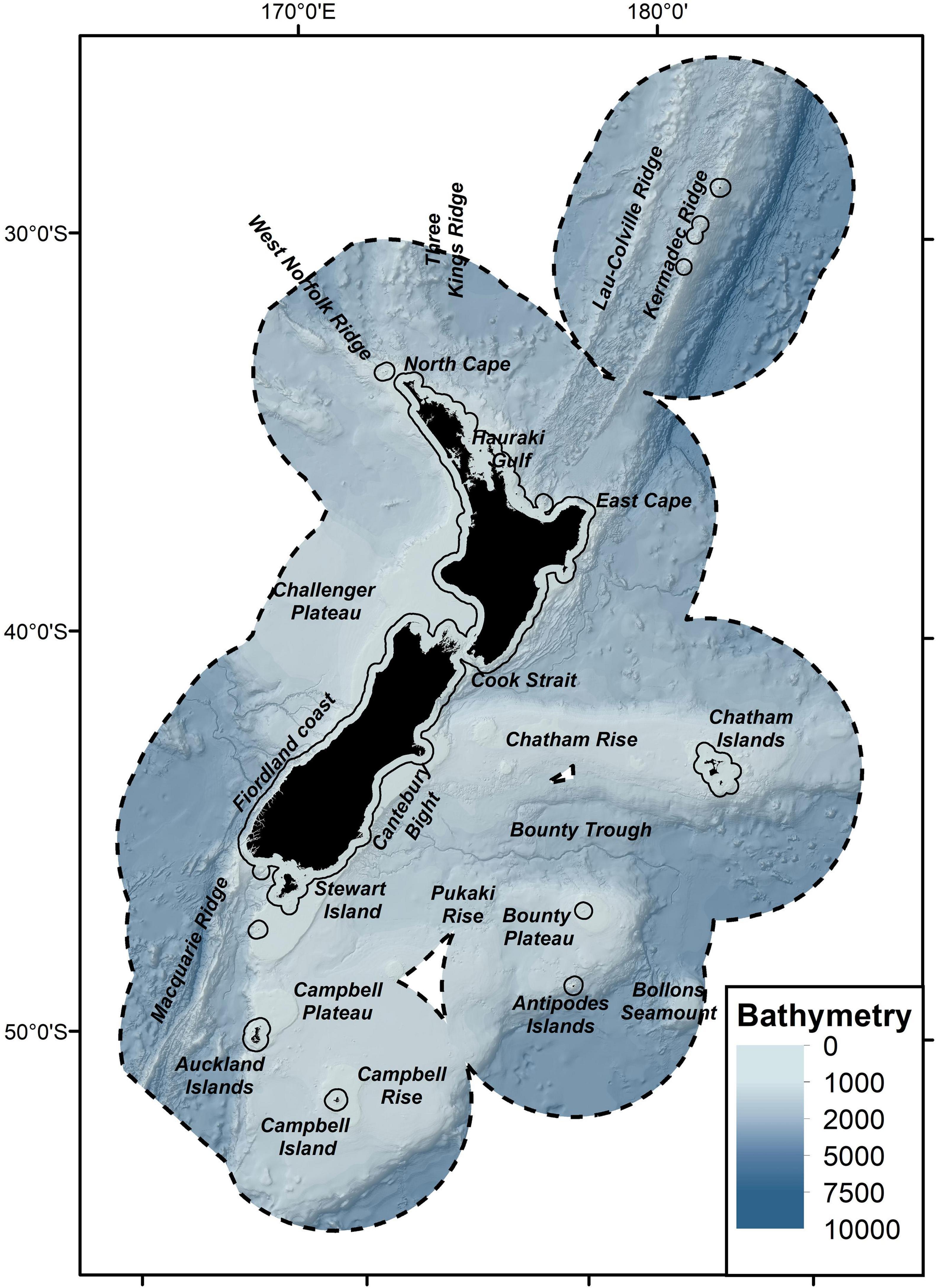
Figure 1. Map of the study region. New Zealand Exclusive Economic Zone (EEZ, black dashed line), Territorial Sea (TS, solid black line), water depth and feature names used throughout the text are displayed.

New Zealand’s marine environment was described using 36 gridded environmental variables (Supplementary Table 1), collated at two resolutions: a 250 m resolution grid from the coastline to the edge of the TS (12 NM from shore), and a 1 km resolution grid from the edge of the TS to the edge of the EEZ (Figure 1). Spatial layers were projected using an Albers Equal Area projection centred at 175°E and 40°S (EPSG:9191). The 36 environmental variables were thought to influence the distribution of benthic and demersal taxa, and therefore distribution of species composition, richness, and turnover (e.g., see Leathwick et al., 2006; Compton et al., 2013; Smith et al., 2013; Anderson et al., 2016; Rowden et al., 2017; Stephenson et al., 2018b; Georgian et al., 2019). Several environmental variables showed some co-linearity within records for biotic groups but all levels of co-linearity were considered acceptable (Pearson correlation < 0.9) for tree-based machine learning methods (Elith et al., 2010; Dormann et al., 2013) and more specifically GF modelling (Ellis et al., 2012).

A subset of twenty environmental variables were selected for GF modelling for all biotic groups (grey rows, Supplementary Table 1) through a model-tuning process which aimed to maximise model fit (see section “Estimating Compositional Turnover”). These were: bathymetry, benthic sediment disturbance, bottom nitrate, dissolved oxygen at depth, bottom phosphate, salinity at depth, bottom silicate, temperature at depth, broadscale Bathymetric Position Index, fine-scale Bathymetric Position Index, chlorophyll-a concentration spatial gradient, detrital absorption, seabed incident irradiance, downward vertical flux of particulate organic matter at the seabed, turbidity, annual amplitude of sea floor temperature, sediment classification, slope, sea surface temperature gradient, and tidal current speed.

In most cases, conventional modelling approaches seek to fit the most parsimonious model and the inclusion of many variables generally only provide minimal improvement in predictive accuracy and complicate interpretation of model outcomes (Leathwick et al., 2006). However, here, the interpretation of model outcomes (i.e., the drivers of distribution) was of secondary interest, the primary focus being on maximising the predictive accuracy of the model.

Biological Data

Occurrence records of four biotic groups (demersal fish, benthic invertebrates, macroalgae, and reef fish) were collated from various sources (Supplementary Table 2). All records were groomed: records located on land, outside the New Zealand marine environment and/or duplicated within and between databases were removed. Taxonomy was standardised across datasets and years to the most recent nomenclature. Demersal fish, reef fish and macroalgae were identified to species level, whereas benthic invertebrates were identified to genera. Further information on the data treatment and assumptions and distributions of taxa records are provided for each biotic group in Supplementary Materials 1.

Records for each of the biotic groups were separately aggregated to unique locations of different spatial resolutions: demersal fish and benthic invertebrates were aggregated to 1 km grid resolution, whereas macroalgae and reef fish taxa (coastal taxa) were aggregated to a 250 m grid resolution. Taxa with ≥10 unique sample locations were retained for the analysis (e.g., Stephenson et al., 2018b) because this ensured that there were sufficient samples to run GF models. Following quality control and spatial aggregation, a total of 630,997 records across the four biotic groups occurring at 39,766 unique locations were retained for final analysis. Values for environmental variables were derived for each taxa record location by overlaying them onto the environmental predictor layers using the “raster” package in R (Hijmans and van Etten, 2012). For demersal fish and benthic invertebrate records this procedure was undertaken using 1 km grid resolution environmental variables (including in areas where information was available at a 250 m grid resolution in order to match the spatial scale at which these were sampled), whereas environmental values for reef fish and macroalgae records were extracted from the 250 m grid resolution environmental variables.

Demersal fish, macroalgae, and reef fish were collected using consistent methods for each of the biotic groups (e.g., demersal fish were collected by research trawls). In contrast, benthic invertebrate records were collected using a variety of sampling methods (208 different gear types). Many of the gear types used were name variants of commonly used sampling gear types, but for most records, the specific sampling parameters (e.g., mesh size, tow length, etc.) were not recorded. In order to account for both the large number of gear types recorded and the differences in sampling parameters, gear types were grouped into “catchability categories.” Catchability was assumed to be influenced by gear size, deployment area and selectivity (Supplementary Table 3; Stephenson et al., 2018a). Sampling gear types were assigned codes for each of the catchability categories (Supplementary Table 4). Out of 18 possible catchability categories, the available invertebrate samples occurred in six categories: LLG – Large gear types, deployed over large areas, which were not selective (e.g., otter trawls); LMG – Large gear types, deployed over medium-sized areas, which were not selective (e.g., beam trawls); MMG – Medium sized gear types, sampling medium sized areas, which were not selective (e.g., benthic sled); SMG – Small gear types, sampling medium sized areas, which were not selective (e.g., Devonport dredge); SMHS – Small gear types, sampling medium sized areas, which were highly selective (e.g., collected by hand, bottom longline); SSG – Small gear types, sampling small areas, which were not selective (e.g., box corer). Records of LLG and LMG were combined as these catchability categories represent commercial fishing practices with similar catches of invertebrates likely to be more demersal in nature (i.e., some squid species). All records collected from highly selective gear catchability category (e.g., SMHS) were excluded from the analysis, because methods classified within this category were considered too variable to provide reliable records of absence (20,010 records were excluded across 412 genera and 2,097 unique locations, including 190 genera unique to selective methods).

Estimating Compositional Turnover

For the demersal fish, macroalgae, and reef fish biotic groups, and for the four benthic invertebrate catchability categories (LLG.LMG, MMG, SMG, and SSG), GF models were fitted using the “extendedForest” (Liaw and Wiener, 2002) and “gradientForest” (Ellis et al., 2012) R packages. GF model aggregates results from a collection of Random Forest (RF) models (Breiman, 2001), each of which describes the environmental relationships of an individual species. Information from the individual Random Forest models about the relative importance of each environmental predictor, and information on where changes in the presence (or abundance) of the modelled species occur along their environmental ranges is aggregated to generate a transformed set of environmental predictors that represent species turnover (Pitcher et al., 2012).

GF models were fitted with 500 trees and default settings for the correlation threshold used in the conditional importance calculation of environmental variables. For each of the 7 GF models, we extracted information on the predictive power of the individual RF models (R²_f for each taxon measured as the proportion of out-of-bag variance explained) (Ellis et al., 2012) and the importance of each environmental variable (R² assessed by quantifying the degradation in performance when each environmental variable was randomly permuted¹ (Pitcher et al., 2012). The environmental variables used in each GF model were selected to maximise the number of taxa effectively modelled (i.e., taxa with R²_f > 0) and increase model fits for the most poorly modelled taxa (i.e., taxa with low R²_f).

Gradient forest aggregates the values of the tree-splits from the RF models for all taxon models with positive fits (R²_f > 0) to develop empirical distributions that represent taxa compositional turnover along each environmental gradient (Ellis et al., 2012; Pitcher et al., 2012). The turnover function is measured in dimensionless R² units, where taxa with highly predictive random forest models (high R²_f values) have greater influence on the turnover functions than those with low predictive power (lower R²_f). The shapes of these monotonic turnover curves describe the rate of compositional change along each environmental predictor; steep parts of the curve indicate fast assemblage turnover, and flatter parts of the curve indicate more homogenous regions (Ellis et al., 2012; Pitcher et al., 2012; Compton et al., 2013).

The use of the dimensionless R² to quantify compositional turnover enables information from multiple taxa to be combined, even if that information comes from different sampling devices, surveys or regions (Ellis et al., 2012). In the first instance, the compositional turnover functions from each of the benthic invertebrate catchability category GF models were combined using the “combinedGradientForest()” function to provide a combined benthic invertebrate GF model (hereafter referred to simply as “benthic invertebrate” GF model). In the second instance, a final combined GF model was created using the “combinedGradientForest()” function across all biotic groups (demersal fish, reef fish, benthic invertebrates, and macroalgae), which we hereafter refer to as the “community” model. Broadly, this method of combining GF models accounts for the number of taxa, the number of samples, and the taxa R²_f along the gradient of each environmental variable from individual GF models to provide a cumulative estimate of compositional turnover [for further details see, Ellis et al. (2012) and Pitcher et al. (2012)].

The compositional turnover functions from each biotic group and the community GF models (shapes of the turnover curves) were used to transform the gridded environmental layers (both 250 m and 1 km grid resolutions), creating a “transformed environmental space” representing compositional turnover. Variation within this transformed environmental space was summarised using principal components analysis (PCA) (Pitcher et al., 2011). The colours used in the PCA of each biotic group/community model were based on the first three axes of their respective PCA analysis so that similarities/differences in colour corresponded broadly to pairwise similarities/differences in the transformed environmental space and thus, by inference, describe differences in taxa composition (Stephenson et al., 2018b). Predicted taxa compositional turnover for each biotic group and community model was plotted geographically using the colour scheme derived from their respective PCA analyses.

GF models for each biotic group, as well as the community GF model, were bootstrapped 100 times. That is, 100 community GF models were fitted (as for the main model described above) to separate randomly selected subsets of the full input dataset. For biotic groups with ≥5,000 samples (Supplementary Table 2), a random selection of 5,000 samples was selected from the full dataset. This number of samples was selected both to ensure reasonable computational time for the analysis, and because previous analysis using demersal fish data indicated that this number of samples provided stable (consistent) model outputs (Stephenson et al., 2018b). For biotic groups with <5,000 samples (Supplementary Table 2), 75% of the dataset was randomly selected for each bootstrap iteration. The bootstrapping process was repeated 100 times, and at each iteration, species compositional turnover functions were used to transform the gridded environmental layers (both 250 m and 1 km grid resolutions). Mean (±1 standard deviation of the mean) estimates of taxa R²_f and environmental variable importance (R²) were calculated for each GF model from the 100 bootstrapped iterations.

Spatial Predictions and Uncertainty

Spatial estimates of compositional turnover from each GF model (i.e., for each biotic group and community model), were averaged (mean). A spatially explicit measure of uncertainty [measured as the standard deviation of the mean (SD) compositional turnover averaged across each environmental variable] was calculated for each grid cell using the 100 bootstrapped transformed environmental layers.

As an added measure of model uncertainty, for each GF model, we estimated “coverage of the environmental space” (Smith et al., 2013; Stephenson et al., 2020c). The “environmental space” is the multidimensional space produced by considering each of the environmental variables as a dimension. Some parts of this environmental space will contain many samples – meaning we can be more confident of the relationships and the predictions (Smith et al., 2013) – while other parts will contain few samples. Predictions for the less sampled parts of the environmental space are considered less reliable, and should be interpreted with greater caution (Smith et al., 2013). We modelled variation in sampling density within the environmental space by combining our samples (assigned as “present”) with an equal number of randomly sampled values from the environmental space (i.e., where we did not have any taxonomic samples – assigned as “absences”). A Boosted Regression Tree (BRT; Elith et al., 2006) model was then used to model the relationship between these “present” (true) samples and “absent” (random) samples for the 20 environmental variables used in the GF analyses. The “Dismo” package (Hijmans et al., 2017) was used with BRT models fitted using a Bernoulli error distribution, a learning rate that yielded 2,000 trees and an interaction depth of 2 (so that only pair-wise combinations of the environmental variables were considered). Predictions using this model yielded estimates of the probability of a sample occurring in each part of the environmental space, these estimates ranging between 0 and 1, where 0 indicated very low sampling of the environmental space and 1 a very high level of sampling (Stephenson et al., 2020c).

Defining the Classification

The mean spatial estimate of compositional turnover from the community GF model (i.e., the bootstrapped GF model which included samples from all biotic groups) was classified using a two-stage approach (Leathwick et al., 2011; Stephenson et al., 2018b) using the R package “cluster” (Maechler et al., 2017). For the first stage, mean spatial estimates of compositional turnover were clustered to form 500 initial groups using non-hierarchical, k-medoids clustering. Average values for the transformed environmental predictors were then computed for each of these initial groups. For the second stage, a hierarchical clustering approach – flexible unweighted pair group method with arithmetic mean (UPGMA) – using the Manhattan metric, and a value for beta of -0.1 (Belbin et al., 1992) was used to define each group from the initial 500. This second classification step was undertaken at various levels of classification detail ranging from 5 to 150-group levels in increments of 5 representing seafloor communities at various spatial scales.

Given the hierarchical nature of the GF-based classification, the most appropriate level of classification detail for planning purposes will vary depending on the spatial scale of the application and the level of information required for management. Using the biological data included in the GF models, the discrimination across classification levels was assessed [5–150 groups in increments of 5, e.g., as in Snelder et al. (2007)] using an analysis of similarities test (ANOSIM) analysis (Clarke and Warwick, 2001). The global R statistic was calculated as the difference in ranked biological similarities arising from all pairs of replicate sites between different groups, and the average of all rank similarities within groups, adjusted by the total number of sites. Global R is equal to 1 if all replicates within groups are more like each other than any replicates from different groups and is approximately 0 if there is no group structure. Significance levels of the ANOSIM statistics were tested with a randomisation procedure based on the null hypothesis of no group structure. All ANOSIM analyses were undertaken in R using the “Vegan” package (Oksanen et al., 2013). We only analysed groups with adequate biological data (≥5 unique occurrences). Group means for each of the transformed environmental variables were calculated and plotted in a PCA and geographical distributions were plotted for each classification from 5 to 150 groups (Supplementary Materials 2).

Finally, we describe the 75-group level classification in greater detail. We refer to this classification as the New Zealand “Seafloor Community Classification” (NZ SCC). This classification level represented the highest number of groups that captured the majority of the variation across the New Zealand marine environment, based on examining the ANOSIM global R statistic for each classification group, and which contained an adequate number of biological records (see “Results” below). Following methods developed by Stephenson et al. (2020a), individual classification group descriptions for the New Zealand SCC (75-group classification) are provided in Supplementary Materials 3. This included: (1) The location of the New Zealand SCC group within the New Zealand marine environment. (2) Descriptions of a subset of each groups’ environmental characteristics, termed “characterising environmental conditions.” (3) Descriptions of each groups’ biological characteristics, calculated as mean frequency occurrence of each taxon within classification groups and investigating the contribution of individual taxa to intra-group similarity (SIMPER analysis using Bray-Curtis similarity, in PRIMER v7.0.13) (Stephenson et al., 2020a). Characterising species were defined as those species contributing more than 4% to the SIMPER intra-group similarity. (4) A measure of model confidence, for each classification group, represented by the mean, 25 and 75% quantile for the uncertainty estimate of compositional turnover (SD of the combined bootstrapped GF) and the overall predicted environmental coverage.

Results

Compositional Turnover and Uncertainty

Models were able to be fitted for most taxa across all biotic groups (i.e., R²_f > 0, Table 1). However, individual taxon R²_f values varied widely, ranging from 0.19 (macroalgae, Table 1) to 0.94 (reef fish, Table 1). On average, the GF models explained 47–53% of variation in occurrence across biotic groups (mean taxa R²_f: 0.47–0.53, Table 1).

TABLE 1

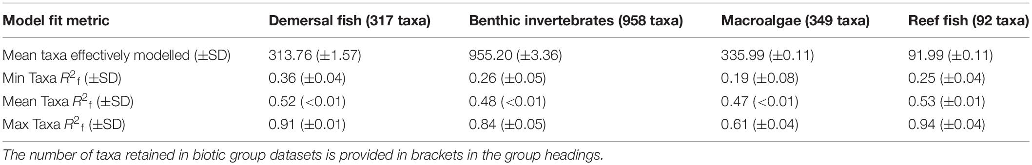
Table 1. Mean (±SD) model fit metrics of individual taxa (R²_f) from bootstrapped gradient forest (GF) models.

Although all environmental variables contributed to predicting compositional turnover for all models (positive R², Supplementary Table 5), their relative importance (in terms of mean cumulative importance) varied across biotic groups. The most consistently important variables in the biotic group GF models were dissolved oxygen at depth and bottom salinity (Supplementary Table 5). Tidal current speed was important in GF models of demersal fish, benthic invertebrates and the community GF model. Many of the environmental variables had moderate cumulative importance across all biotic groups and in the community GF model, e.g., dissolved oxygen at depth, seabed incident irradiance, downward vertical flux of POC at the seabed (R²: 0.0015–0.004, Supplementary Table 5). The predicted cumulative changes in compositional turnover along each environmental variable for each biotic group and the overall community are presented in Supplementary Materials 1.

Spatial patterns in overall community compositional turnover reflected broadscale patterns in environmental variables linked to well-defined oceanographic patterns observed in New Zealand’s waters. Briefly, compositional turnover was minimal in the deepest water (>2,000 m), although with progression into shallower waters (1,000–2,000 m) there appeared to be differences in taxa occurring in the northwest of the study area compared to all other deep-water areas (Figure 2). With progression into intermediate depths (70–1,000 m), there was a clear latitudinal separation in taxa composition along the boundaries of the Subtropical Front (STF), a highly productive zone of mixing between high salinity, nutrient poor, warm, northern waters, and low salinity, nutrient rich, cold, and southern waters (Bradford-Grieve et al., 2006; Leathwick et al., 2006, 2012; Stephenson et al., 2018b; Figure 2). In shallow water (0–70 m), patterns in community compositional turnover were more closely associated both with latitude and with more localised environmental conditions. Namely, turbidity, tidal currents, and broadscale and fine-scale Bathymetric Position Index (Figure 2).

FIGURE 2

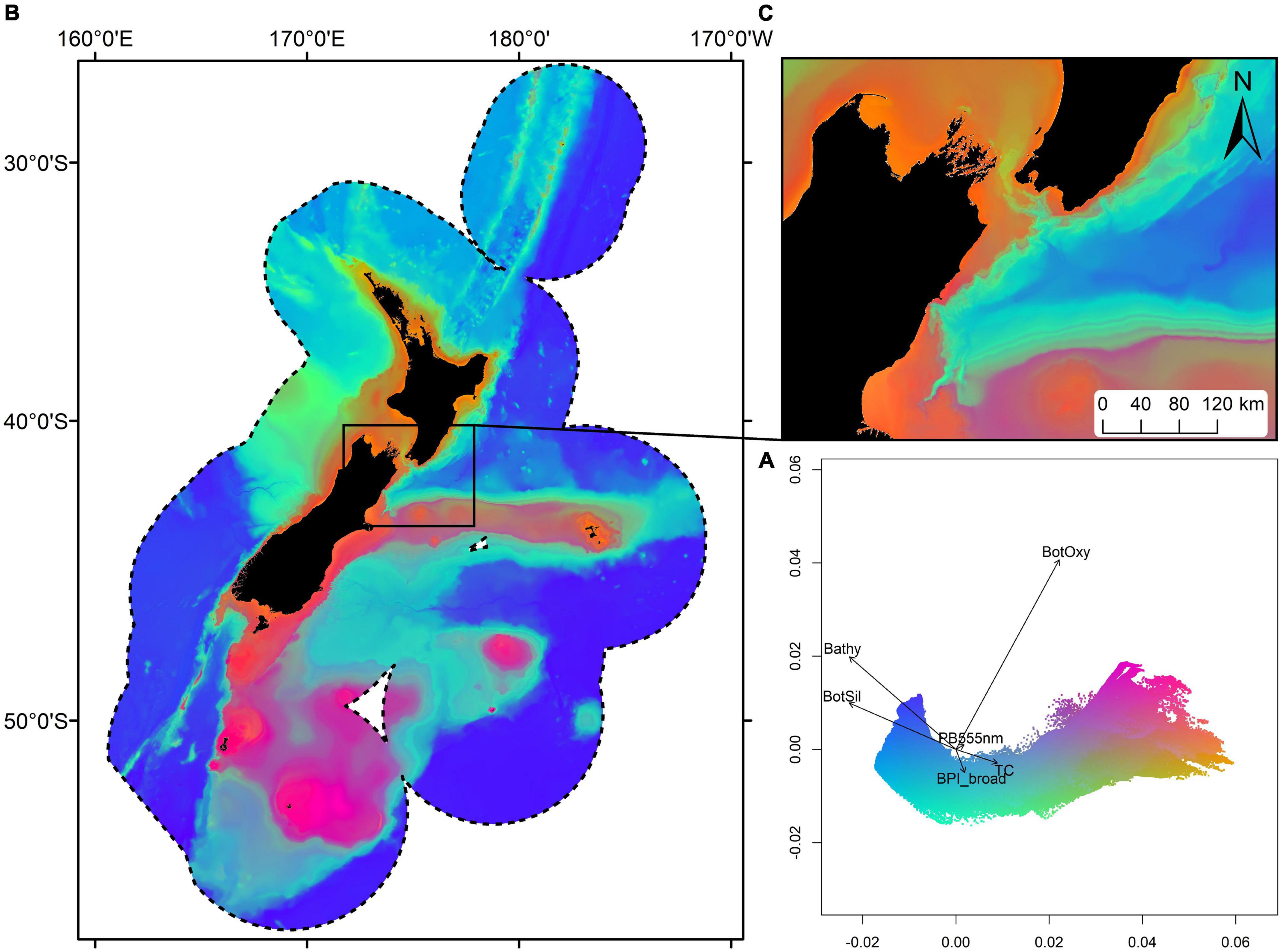
Figure 2. Mean predicted community compositional turnover in geographic and principal components analysis (PCA) space derived from combined bootstrapped Gradient Forest models fitted using samples from all biotic groups. Colours are based on the first three axes of a PCA analysis so that similarities/differences in colour correspond broadly to similarities/differences in predicted compositional turnover. Compositional turnover in PCA space, with vectors indicating correlations with the six most important environmental predictors (A); Geographic distributions of community compositional turnover across the New Zealand marine environment (dashed line) (B); Geographic distribution of community compositional turnover at finer scales, centred on Cook Strait (C). See Figure 1 for feature names.

The SD for all GF models was low compared to the mean compositional turnover, i.e., the uncertainty in the compositional turnover was low even for the most variable areas. The SD of mean compositional turnover for the community GF model was highest close to shore in areas of high compositional turnover, for example, in Cook Strait and the Marlborough Sounds (Figure 3A). Much of the continental shelf (areas shallower than 200 m) and the Chatham Rise displayed moderate to high variability in mean compositional turnover (Figure 3A). Deep water areas (>2,000 m) displayed the lowest variability in mean compositional turnover, in part reflecting the relative environmental homogeneity associated with these abyssal waters, but also likely reflecting, at least in part, the relative lack of sampling in these areas as environmental coverage was low for most areas deeper than 2,000 m (Figures 3A,B). Environmental coverage was high in areas close to shore and along the Chatham Rise (Figure 3B) and moderate for parts of the Challenger and Campbell plateaus (Figure 3B).

FIGURE 3

Figure 3. Spatially explicit estimate of uncertainty and environmental coverage from the combined bootstrapped Gradient Forest model fitted using samples from all biotic groups. Uncertainty estimate (SD) of compositional turnover modelled using bootstrapped Gradient Forest model fitted with demersal fish, benthic invertebrate, macroalgae and reef fish samples (A). Predicted environmental coverage depicting the confidence that can be placed in the predictions, ranging from low (i.e., no samples in the dataset with those environmental conditions) to high (i.e., many samples with those environmental conditions) within the New Zealand marine environment (B). See Figure 1 for feature names.

Seafloor Community Classification

Assessment of Classification Strength

There was adequate unique occurrences of benthic invertebrate and demersal fish (i.e., ≥5 unique occurrences in a given group) for more than 70% of all groups (up to 150 groups, Table 2), however, for the more coastally restricted taxa from the macroalgae and reef fish biotic groups, there were fewer groups with adequate occurrences (Table 2). All the global ANOSIM R values were significant at the 1% level. The global R values generally increased for all data sets as the classification detail was increased, indicating that finer levels of classification detail defined more biologically distinctive environments (Table 2). The ANOSIM R values were higher for demersal and reef fish classifications than those for the benthic invertebrates and the macroalgae. However, the classification strength became more gradual for all biotic groups, once the number of classification groups exceeded 55–75 groups (Table 2). Furthermore, pairwise differences between groups (with adequate sample number) declined with increasing classification detail (Table 2).

TABLE 2

Table 2. Results of the pair-wise analysis of similarities test (ANOSIM) analysis for the biotic groups at varying levels of classification detail.

The New Zealand Seafloor Community Classification

The 75-group classification – termed the New Zealand SCC – was used because it was the highest number of groups that captured the majority of the variation across the New Zealand marine environment (as assessed by global ANOSIM R values) and contained an adequate number of biological records. The New Zealand SCC exhibited clear differences in terms of environmental conditions (summarised in Figure 4) and geographic distributions (Figures 5, 6). Not surprisingly, geographic and environmental patterns of the New Zealand SCC closely reflect the patterns of the community compositional turnover on which the New Zealand SCC was based. At broad scales, New Zealand SCC groups were differentiated primarily according to oceanographic conditions such as depth (along PC1 in Figure 4) and bottom temperature (co-linear with bottom salinity and bottom oxygen, along PC2 in Figure 4). Environmental differences among New Zealand SCC groups in deep water (groups 1–19, mean depths between 4,156 and 537 m) were relatively muted, but greater environmental differences were evident among New Zealand SCC groups at intermediate depths (group 20–48, primarily mean depths between 537 and 52 m), particularly with respect to bottom temperature, bottom oxygen concentration and bottom salinity. These more pronounced environmental differences among groups at intermediate depths were aligned with well-defined oceanographic patterns observed in New Zealand’s oceans, with a clear latitudinal separation along the boundaries of the Subtropical Front (STF). Intermediate depth groups to the north of the STF included groups 27–35; 41–43 and south of the STF included 20–23; 36–40; 46–48 (Figure 5). Environmental differences became even more pronounced at shallow depths (groups 49–75, primarily mean depths between 54 and 1 m), where variation in more localised environmental conditions such as productivity (downward vertical flux of particulate organic matter at the seabed), seafloor topography (broadscale Bathymetric Position Index and slope), seabed disturbance (benthic sediment disturbance) and tidal currents (Figure 4) were important differentiating factors (Figure 5).

FIGURE 4

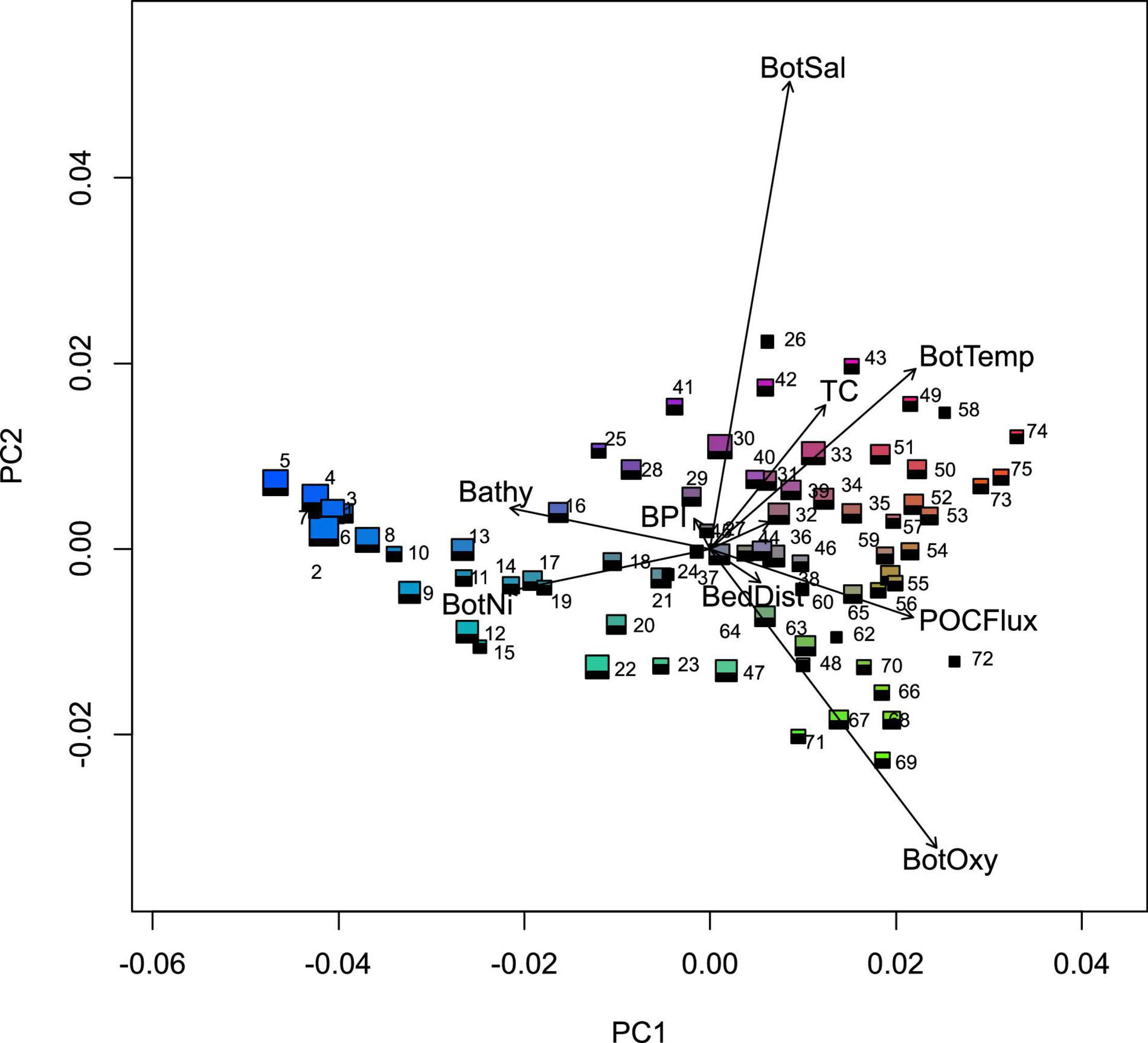
Figure 4. Principal component analysis of the seafloor community classification groups (75 groups) for the New Zealand marine environment. Vectors indicate correlations with the nine most important environmental predictors and symbol size indicates the relative spatial area represented by the group. Colours are based on the first three axes of the PCA analysis applied to the group means for each of the transformed predictor variables, so that similarities/differences in colour correspond broadly to similarities/differences in predicted compositional turnover. Environmental predictors include: bathymetry (Bathy), benthic sediment disturbance (BedDist), bottom nitrate (BotNi), dissolved oxygen at depth (BotOxy), salinity at depth (BotSal), temperature at depth (BotTemp), broadscale Bathymetric Position Index (BPI), downward vertical flux of particulate organic matter at the seabed (POCFlux) and tidal current speed (TC).

FIGURE 5

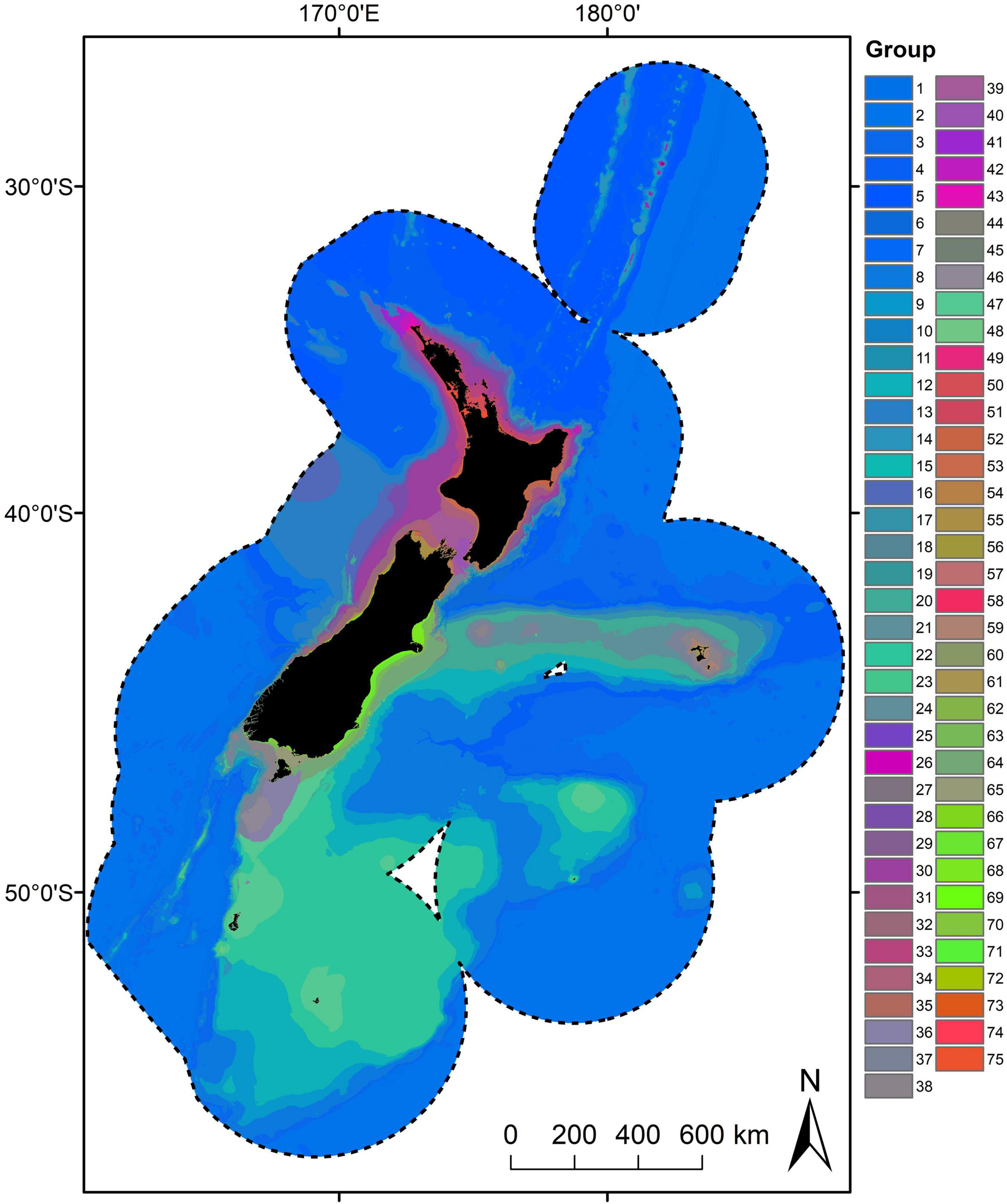
Figure 5. Geographic distribution of the Seafloor Community Classification (75 groups) derived from combined bootstrapped Gradient Forest model. Colours are based on the first three axes of the PCA analysis applied to the group means for each of the transformed predictor variables, so that similarities/differences in colour correspond broadly to similarities/differences in predicted compositional turnover.

FIGURE 6

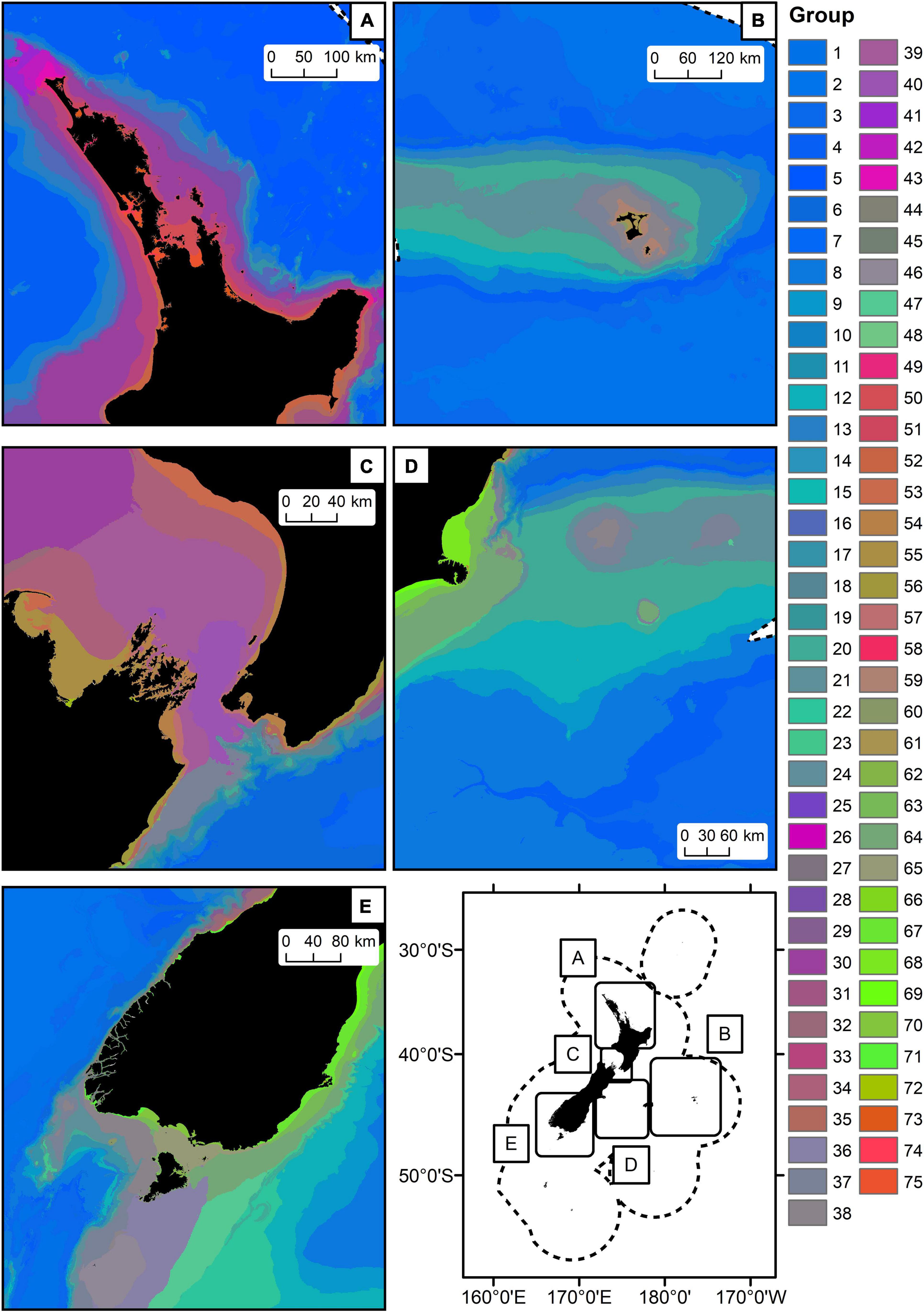
Figure 6. Closeup views of parts of the geographic distribution of the Seafloor Community Classification (75 groups, panels A–E) derived from combined bootstrapped Gradient Forest model. Colours are based on the first three axes of the PCA analysis applied to the group means for each of the transformed predictor variables, so that similarities/differences in colour correspond broadly to similarities/differences in predicted compositional turnover.

Environmental differences between New Zealand SCC groups were mirrored by differences in biological composition. For example, the New Zealand SCC groups varied in their characterising taxa with many taxa occurring in several groups sharing similar environmental characteristics [e.g., orange roughy (Hoplostethus atlanticus), and smooth oreo (Pseudocyttus maculatus) were most frequently observed in deep cold-water groups], whereas a large number of species occurred infrequently or in a small number of groups. A detailed description of the characterising demersal fish, benthic invertebrate, macroalgae, and reef fish characterising taxa is provided in Supplementary Materials 3.

In addition, mean values for the two spatially explicit estimates of uncertainty differed between New Zealand SCC groups (summarised in Supplementary Materials 3). Broadly, with decreasing depth, the mean environmental coverage increased, although some small localised New Zealand SCC groups with few biological samples had low environmental coverage (e.g., group 26). Several New Zealand SCC groups had low or variable number of samples across biotic groups, but moderate to high combined environmental coverage (e.g., shallow coastal groups 58–60, 66, 72), suggesting sampling in similar environmental conditions had occurred for these taxa in other New Zealand SCC groups.

Discussion

The New Zealand SCC developed here is a significant advance on previous numerical classifications, in New Zealand and globally. Firstly, it combined a larger number of taxonomic records (630,997 records of 1,716 taxa occurring at 39,766 unique locations) from multiple biotic groups, across a large area (>4.2 million km²), with a comprehensive and high-resolution set of environmental predictor variables compared to previous studies (e.g., Snelder et al., 2007; Stephenson et al., 2020a). Secondly, because flexible machine learning modelling methods were used, non-linear relationships between taxa and environment were incorporated (Pitcher et al., 2012). For the first time globally, spatial estimates of confidence were provided for the predicted compositional turnover through the use of bootstrapping techniques, which can in turn be used to partially assess the confidence that can be placed in the individual New Zealand SCC groups.

Critical Appraisal of the New Zealand Seafloor Community Classification

The methods and data used to develop the New Zealand SCC build on those used in previous classifications of New Zealand’s marine environment: the New Zealand Marine Environment Classification (MEC, Snelder et al., 2007) and the Benthic Optimised Marine Environment Classification (BOMEC, Leathwick et al., 2012). Although the classification is environment-based, in broad terms the classification can be understood as a spatial summary of variation in seafloor community composition and turnover in the New Zealand marine environment (Stephenson et al., 2020a). Overall, the spatial distribution of the New Zealand SCC is consistent with the MEC and BOMEC which identified depth, and to a lesser extent, water temperature and water mass, and major oceanographic features as important drivers of taxa composition. However, the New Zealand SCC also identified finer-scale environmental differences for community groups at shallow depths, where variation in more localised environmental conditions such as productivity, seafloor topography, seabed disturbance, and tidal currents were important differentiating factors.

The New Zealand SCC groups represent taxa that share the same suite of environmental preferences, and therefore inhabit the same locations. These groups can be considered communities as they describe groups of spatially and temporally co-occurring taxa, which may interact to some extent with one another (Morin, 2009). Some species in a community will interact either directly (e.g., through predator-prey interactions) or indirectly (e.g., by feeding on the same organisms), while other taxa may not necessarily interact with each other and may only be “associated” because they inhabit the same physical space (Francis et al., 2002). There is still a paucity of information with regards to species interactions at the spatial scales of the communities identified by the New Zealand SCC. Nevertheless, the inferred communities from the New Zealand SCC provide useful descriptions of habitat and biotic assemblages for spatial resource management and conservation planning, particularly when considered alongside the estimates of confidence for each of the groups.

Management Application

Describing spatial variation in species compositional turnover and richness is central both to our understanding of the scaling of diversity, and for identification of priority sites for marine spatial planning and conservation (McKnight et al., 2007). New Zealand SCC groups are based on estimated taxa compositional turnover, which allows spatially explicit measures of within-group and between-group similarity in taxonomic composition to be produced (Stephenson et al., 2021a). In turn, these similarity metrics can allow identification of environments that are likely to host rare or unusual communities as well as identifying geographic areas (which may consist of multiple New Zealand SCC groups) that are most representative of New Zealand seafloor communities as a whole, for example, in a spatial conservation prioritisation analysis (Leathwick et al., 2011).

Given the hierarchical nature of the New Zealand SCC classification, consideration will be required as to what constitutes the most appropriate level of classification detail for planning purposes. At the scale of the New Zealand marine environment, the 75-group New Zealand SCC may be appropriate. Using a higher number of classification groups (100–200 groups) is likely to be more appropriate for regional scale management planning, particularly for inshore areas where there is greater heterogeneity in environmental conditions and biological communities (Stephenson et al., 2018b). As part of any spatial planning process, information from the New Zealand SCC could be supplemented with the inclusion of other spatial layers to facilitate selection of areas of particular importance [e.g., see Stephenson et al., 2018a; Lundquist et al., 2020) for a comprehensive list and description of spatial layers available in New Zealand to inform the identification of Key Ecological Areas]. The New Zealand SCC aims to represent seafloor communities; however, to achieve comprehensive representation for marine spatial planning, information on other species, including pelagic species, will likely need to be included. By itself, the New Zealand SCC is unlikely to be an appropriate proxy for pelagic species distributions (Hewitt et al., 2015). Spatial layers relating to other values and uses, such as social, cultural and economic value, would also need to be factored in as part of a marine planning process.

A spatial planning analysis using the 75-group New Zealand SCC would need to include the classification uncertainty measures developed here because failure to acknowledge sources of uncertainty can lead to poor management decisions (Regan et al., 2005; Link et al., 2012). Here we provide two spatially explicit measures of uncertainty: model variability and environmental coverage, which provide two complementary measures to be considered by managers (Stephenson et al., 2021b). The environmental coverage provides an indication of the parts of the environmental space that, for example, contain many samples – meaning we can be more confident of the relationships and the predictions for compositional turnover and SSC groupings in such areas (Smith et al., 2013). The uncertainty estimates of community compositional turnover (i.e., standard deviation of the mean (SD) compositional turnover averaged across each environmental variable) provide an important indication of the variability in the modelling estimates. Given that uncertainty estimates of compositional turnover will only vary in areas where samples are present, we suggest that the uncertainty associated with individual SCC groups first be assessed by examining the number of samples and environmental coverage values. Where these values are adequate [e.g., environmental coverage > 0.05 as in Stephenson et al. (2020c) or another suitable cut-off], the uncertainty estimates of compositional turnover will provide further insight into the variability (and therefore the confidence) of the underlying models used for the classification. However, it should be noted that both of these uncertainty estimates are not propagated through the model to include any uncertainty in the classification. That is, we only quantify parts of the model uncertainty (albeit arguably the most important parts) and there are no estimates of classification uncertainty per se (Hill et al., 2020). This means that for parts of the environmental space our estimate of model uncertainty will be an under-estimate (i.e., particularly for those parts of the environmental space that could be classified as either in one group or another similar group). However, spatial predictions of inter- and intra-group (biological) similarity can be generated from the classification and be used to highlight those areas in the classification groups that may be classified in one group or another and therefore may represent less certain classifications [e.g., see methods and use of these layers in Stephenson et al. (2021a)].

One challenge with numerical classifications, such as the New Zealand SCC, is the communication of results from a statistically complex product in a way that facilitates their use by management agencies and others involved in spatial planning processes (Rowden et al., 2018). Individual group descriptions for the New Zealand SCC are provided in Supplementary Materials 3. These descriptions are provided to facilitate use of the classification by both managers and stakeholders and, at least in part, help bridge the gap between the typical output from numerical classifications and the readily understandable habitat and assemblage descriptions that result from thematic classifications. As new data become available, the underlying numerical methodology underpinning the classification can be updated allowing the New Zealand SCC to be continually improved over time.

Improving the Classification

Despite the large datasets collated for the development of the New Zealand SCC, there remain limitations associated with the classification, which at least in part, can be attributed to the available biological and environmental data. The long temporal span over which taxa samples were collected means that there is a mismatch between the temporal window of biological data and that of the environmental variables which were mostly compiled from data collected in the last few decades. This mismatch means that the compositional turnover presented here should be interpreted as a spatially and temporally smoothed representation (Stephenson et al., 2018b). Furthermore, it is worth noting that data were collected over a time span that includes the establishment of widespread commercial fishing in the region (Baird and Wood, 2018), and the impact of this disturbance on seafloor communities has not been incorporated into the modelling methodology.

Although the species occurrence data we used mostly provided adequate spatial coverage of our study area close to shore and further offshore on the Chatham Rise and the Challenger and Campbell Plateaus (as assessed by the coverage of the environmental space), several large, outlying sections had few or no biological samples, notably the vast majority of waters deeper than 2,500 m. For deeper waters where few samples are available, lower confidence can be placed in the predictions of compositional turnover that underpin the New Zealand SCC.

The “quality” of the available biological data varied by biotic group based on differences in sampling gear and method. Records for demersal fish and reef fish were collected using (relatively) consistent sampling gears and methods (Smith et al., 2013; NIWA, 2014, 2018). Abundance estimates were available for both these biotic groups, and few assumptions were required to use these data as presence/absence in GF models to make them consistent with benthic invertebrate and macroalgae group data. In contrast, multiple sampling gears and methods were used to sample benthic invertebrates, which required division of these data into gear catchability categories. However, it should be noted, that there was a high proportion of unique taxa associated with each gear type and therefore it was deemed important to include each of these because they sampled different parts of the community. Information on sampling methods for macroalgae was not easily available but given their localised nature (collected on or close to shore), this was not deemed to be critical. Neither the benthic invertebrate nor the macroalgal data here can be considered true presence/absence (because of variations in the survey designs used to collect these data), and therefore the classification results from these biotic groups should be used with greater caution [although care was taken to account for differences in the biases associated with sampling method as per Phillips et al. (2009)]. Future iterations of the New Zealand SCC may benefit from being tuned using abundance estimates and, for benthic invertebrates, records at the species level [e.g., using data from comprehensive surveys as in Bowden et al. (2019)]. Despite these limitations, the taxa data used here form a valuable dataset that will have uses outside the development of the New Zealand SCC (e.g., see Lundquist et al., 2020) and represents the best available compiled biotic information at present for the New Zealand marine environment. The ability of the classification to represent variation in taxa composition at different scales using independent or newly collected data [e.g., as in Bowden et al. (2011) or as in Stephenson et al. (2018b)] would be of interest in order to independently validate the accuracy of the New Zealand SCC.

The lack of consistent spatially explicit abundance information, means that despite the comprehensive SCC group descriptions of the environmental and biotic characteristics, SCC groups may still lack some of the key features that stakeholders may more readily associate with, or understand as habitats and communities. For example, the lack of abundance information means there is no spatial information about the locations of biogenic habitats, despite biogenic habitat forming taxa being present (and identified as characterising taxa) in several groups (e.g., bivalves, stony corals – see Supplementary Materials 3).

Conclusion

The New Zealand SCC and associated spatially explicit uncertainty layers are particularly well suited as inputs for marine spatial planning, and more specifically, marine protection planning and reporting at regional and national scales. Firstly, spatially explicit estimates of within and between group similarity of the New Zealand SCC make it particularly well suited to support developing an effective network of marine protected areas and other tools [goal 10.6.3 of Te Mana o te Taiao – The Aotearoa New Zealand Biodiversity strategy, Department of Conservation (2020)] and complement work currently underway to map Key Ecological Areas within New Zealand’s marine environment. Secondly, the development of two spatially explicit measures of uncertainty allow for the nuanced use of the New Zealand SCC in a marine spatial planning context. Thirdly, the New Zealand SCC summarises a large and complex dataset spanning four sea-floor biotic groups in a single community classification layer that could greatly facilitate communication of complex spatial biodiversity patterns during participatory stakeholder processes. Despite the advances and utility of the New Zealand SCC for conservation planning, there remain several limitations, including a lack of abundance data, and the identification of the key features that some stakeholders may more readily associate with, or understand as, habitats and communities. These limitations can, at least in part, be overcome through the use of other spatial layers to complement the New Zealand SCC (e.g., as collated for the identification of Key Ecological Areas, Stephenson et al., 2018a; Lundquist et al., 2020) such as spatial estimates of fish spawning grounds and biogenic habitats.

Data Availability Statement

The datasets presented in this study can be found in online repositories. The names of the repository/repositories and accession number(s) can be found below: https://doc-deptconservation.opendata.arcgis.com/documents/4050708cbf274e26a978448c4caf2b3d.

Author Contributions

FS, AR, TB, RB, DB, DC, BG, KN, KM, MP, OA, RG, SM, and WN collated and groomed the biological and environmental data. FS, TB, GP, and JL led the data analysis with input from CL, AR, SG, GF, DF, KT, PT, IT, and JH. FS, TB, SW, GP, and JL produced the figures. FS, AR, TB, GP, and JH led the writing, but all authors contributed to the development of ideas, writing and editing of this article, and approved the submitted version.

Funding

This work was funded by the New Zealand Department of Conservation (contract number DOC19208 to NIWA), with additional support from NIWA Coasts and Oceans Research Programmes 4 and 5 (SCI 2020/21).

Conflict of Interest

The authors declare that the research was conducted in the absence of any commercial or financial relationships that could be construed as a potential conflict of interest.

Publisher’s Note

All claims expressed in this article are solely those of the authors and do not necessarily represent those of their affiliated organizations, or those of the publisher, the editors and the reviewers. Any product that may be evaluated in this article, or claim that may be made by its manufacturer, is not guaranteed or endorsed by the publisher.

Acknowledgments

We gratefully acknowledge the input and collegiality of the members of the Marine Protected Areas Science Advisory Group throughout the multiple workshops organised to discuss the scope and methods of the analyses. In addition, we would like to thank Clinton Duffy, Megan Oliver, Constance Nutsford, and Ben Sharp for their thoughts and input throughout this research. We also thank Roland Pitcher for early discussions on the application of Gradient Forest models and Mark Costello and Nicole Hill for their constructive and insightful comments on a prior version of this manuscript. We acknowledge prior research and the methodological developments by New Zealand researchers on which this work builds upon. Namely, the Marine Environment Classification (MEC – Snelder et al., 2007) and the Benthic Optimised Marine Environment Classification (BOMEC – Leathwick et al., 2012), and developments of gradient forest approaches for application in New Zealand funded by the MBIE Sustainable Seas National Science Challenge (Stephenson et al., 2018a,b, 2020c,2021b). This manuscript builds on a report available at https://www.doc.govt.nz/globalassets/documents/conservation/marine-and-coastal/marine-protected-areas/development-of-new-zealand-seafloor-community-classification.pdf (Stephenson et al., 2020b). We acknowledge the contributions of data and advice from many sources including: the National Institute of Water and Atmospheric Research (NIWA) for collections data and spatial environmental variable layers; Auckland and Te Papa Museums for providing collections data; the Department of Conservation for spatial data layers; MODIS data were used courtesy of NASA Goddard Space Flight Center, MODIS project. Ocean colour satellite data were accessed via the NASA Ocean Biology Distributed Active Archive Center (OB.DAAC). Coastal ocean colour data were processed courtesy of Simon Wood (NIWA). We acknowledge the contribution of taxonomic expertise from a very large number of national and international colleagues, too many to individually name, that have provided decades of knowledge and the species names and identifications that we rely on for this work.

Supplementary Material

The Supplementary Material for this article can be found online at: https://www.frontiersin.org/articles/10.3389/fmars.2021.792712/full#supplementary-material

Footnotes

1. ^ Note that R² described by Ellis et al. (2012) and Pitcher et al. (2012) refers to a unitless measure of cumulative importance and should not be confused with the more commonly used R-squared (R²) denoting coefficient of determination.

References

Anderson, O. F., Guinotte, J. M., Rowden, A. A., Tracey, D. M., Mackay, K. A., and Clark, M. R. (2016). Habitat suitability models for predicting the occurrence of vulnerable marine ecosystems in the seas around New Zealand. Deep Sea Res. Part I Oceanog. Res. Papers 115, 265–292. doi: 10.1016/j.dsr.2016.07.006

CrossRef Full Text | Google Scholar

Arponen, A., Moilanen, A., and Ferrier, S. (2008). A successful community-level strategy for conservation prioritization. J. Appl. Ecol. 45, 1436–1445.

Google Scholar

Baird, S. J., and Wood, B. A. (2018). Extent of Bottom Contact by New Zealand Commercial Trawl Fishing for Deepwater Tier 1 and Tier 2 Target Fishstocks, 1989–90 to 2015–16. New Zealand Aquatic Environment and Biodiversity Report No. 193.

Google Scholar

Belbin, L., Faith, D. P., and Milligan, G. W. (1992). A comparison of two approaches to beta-flexible clustering. Multivariate Behav. Res. 27, 417–433. doi: 10.1207/s15327906mbr2703_6

PubMed Abstract | CrossRef Full Text | Google Scholar

Bowden, D. A., Anderson, O., Escobar-Flores, P., Rowden, A., and Clark, M. (2019). Quantifying Benthic Biodiversity: Using Seafloor Image Data to Build Single-Taxon and Community Distribution Models for Chatham Rise, New Zealand. Aquatic Environment and Biodiversity Report No. 235.

Google Scholar

Bowden, D. A., Compton, T., Snelder, T., and Hewitt, J. (2011). Evaluation of the New Zealand Marine Environment Classifications Using Ocean Survey 20/20 Data From Chatham Rise and Challenger Plateau. New Zealand Aquatic Environment and Biodiversity Report No. 77.

Google Scholar

Bradford-Grieve, J., Probert, K., Lewis, K., Sutton, P., Zeldis, J., and Orpin, A. (2006). New Zealand Shelf Region. Cambridge, MA: Harvard University Press.

Google Scholar

Breiman, L. (2001). Random forests. Machine Learn. 45, 5–32. doi: 10.1023/A:1010933404324

CrossRef Full Text | Google Scholar

Clarke, K. R., and Warwick, R. M. (2001). Change in Marine Communities: An Approach to Statistical Analysis and Interpretation, 2nd Edn. Plymouth: PRIMER-E

Google Scholar

Compton, T. J., Bowden, D. A., Roland Pitcher, C., Hewitt, J. E., and Ellis, N. (2013). Biophysical patterns in benthic assemblage composition across contrasting continental margins off New Zealand. J. Biogeogr. 40, 75–89. doi: 10.1111/j.1365-2699.2012.02761.x

CrossRef Full Text | Google Scholar

Department of Conservation (2020). Te Mana O Te Taiao Aotearoa New Zealand Biodiversity Strategy 2020. Wellington: Department of Conservation.

Google Scholar

Dormann, C. F., Elith, J., Bacher, S., Buchmann, C., Carl, G., Carré, G., et al. (2013). Collinearity: a review of methods to deal with it and a simulation study evaluating their performance. Ecography 36, 27–46.

Google Scholar

Dunstan, P. K., Althaus, F., Williams, A., and Bax, N. J. (2012). Characterising and predicting benthic biodiversity for conservation planning in deepwater environments. PloS one 7:e36558. doi: 10.1371/journal.pone.0036558

PubMed Abstract | CrossRef Full Text | Google Scholar

Elith, J., Graham, C. H., Anderson, R. P., Dudík, M., Ferrier, S., Guisan, A., et al. (2006). Novel methods improve prediction of species’ distributions from occurrence data. Ecography 29, 129–151.

Google Scholar

Elith, J., Kearney, M., and Phillips, S. (2010). The art of modelling range-shifting species. Methods Ecol. Evolu. 1, 330–342.

Google Scholar

Ellingsen, K. E., Hewitt, J. E., and Thrush, S. F. (2007). Rare species, habitat diversity and functional redundancy in marine benthos. J. Sea Res. 58, 291–301.

Google Scholar

Ellis, N., Smith, S. J., and Pitcher, C. R. (2012). Gradient forests: calculating importance gradients on physical predictors. Ecology 93, 156–168. doi: 10.1890/11-0252.1

CrossRef Full Text | Google Scholar

Ferrier, S., Manion, G., Elith, J., and Richardson, K. (2007). Using generalized dissimilarity modelling to analyse and predict patterns of beta diversity in regional biodiversity assessment. Diversity Distr. 13, 252–264. doi: 10.1371/journal.pone.0131728

PubMed Abstract | CrossRef Full Text | Google Scholar

Francis, M. P., Hurst, R. J., McArdle, B. H., Bagley, N. W., and Anderson, O. F. (2002). New Zealand demersal fish assemblages. Environ. Biol. Fish. 65, 215–234.

Google Scholar

Georgian, S. E., Anderson, O. F., and Rowden, A. A. (2019). Ensemble habitat suitability modeling of vulnerable marine ecosystem indicator taxa to inform deep-sea fisheries management in the South Pacific Ocean. Fish. Res. 211, 256–274. doi: 10.1016/j.fishres.2018.11.020

CrossRef Full Text | Google Scholar

Gregr, E. J., and Bodtker, K. M. (2007). Adaptive classification of marine ecosystems: identifying biologically meaningful regions in the marine environment. Deep Sea Res. Part I Oceanogr. Res. Papers 54, 385–402. doi: 10.1016/j.dsr.2006.11.004

CrossRef Full Text | Google Scholar

Hewitt, J. E., Wang, D., Francis, M., Lundquist, C., and Duffy, C. (2015). Evaluating demersal fish richness as a surrogate for epibenthic richness in management and conservation. Div. Distr. 21, 901–912.

Google Scholar

Hijmans, R. J., and van Etten, J. (2012). raster: Geographic Analysis and Modeling With Raster Data. R Package Version 2.0-12.

Google Scholar

Hijmans, R. J., Phillips, S., Leathwick, J., and Elith, J. (2017). dismo: Species Distribution Modeling R package version 1.1-4.

Google Scholar

Hill, N., Woolley, S. N. C., Foster, S., Dunstan, P. K., McKinlay, J., Ovaskainen, O., et al. (2020). Determining marine bioregions: a comparison of quantitative approaches. Methods Ecol. Evolu. 11, 1258–1272.

Google Scholar

Hortal, J., de Bello, F., Diniz-Filho, J. A. F., Lewinsohn, T. M., Lobo, J. M., and Ladle, R. J. (2015). Seven shortfalls that beset large-scale knowledge of biodiversity. Ann. Rev. Ecol. Evolu. Syst. 46, 523–549. doi: 10.1146/annurev-ecolsys-112414-054400

CrossRef Full Text | Google Scholar

Leathwick, J., Elith, J., Francis, M., Hastie, T., and Taylor, P. (2006). Variation in demersal fish species richness in the oceans surrounding New Zealand: an analysis using boosted regression trees. Mar. Ecol. Prog. Ser. 321, 267–281. doi: 10.3354/meps321267

CrossRef Full Text | Google Scholar

Leathwick, J., Rowden, A., Nodder, S., Gorman, R., Bardsley, S., Pinkerton, M., et al. (2012). “A Benthic-Optimised Marine Environment Classification (BOMEC) for New Zealand Waters”, New Zealand Aquatic Environment and Biodiversity Report; ISSN 1176-9440.

Google Scholar

Leathwick, J., Snelder, T., Chadderton, W., Elith, J., Julian, K., and Ferrier, S. (2011). Use of generalised dissimilarity modelling to improve the biological discrimination of river and stream classifications. Fresh. Biol. 56, 21–38. doi: 10.1111/j.1365-2427.2010.02414.x

CrossRef Full Text | Google Scholar

Liaw, A., and Wiener, M. (2002). Classification and regression by random forest. R News 2, 18–22.

Google Scholar

Link, J. S., Ihde, T., Harvey, C., Gaichas, S. K., Field, J., Brodziak, J., et al. (2012). Dealing with uncertainty in ecosystem models: the paradox of use for living marine resource management. Prog. Oceanogr. 102, 102–114.

Google Scholar

Lundquist, C., Stephenson, F., McCartain, L., Watson, S., Brough, T., and Nelson, W. (2020). Evaluating Key Ecological Areas Datasets for the New Zealand Marine Environment. NIWA Report Repared for Department of Conservation (2020109HN). New Zealand: Hamilton.

Google Scholar

Maechler, M., Rousseeuw, P., Struyf, A., Hubert, M., and Hornik, K. (2017). cluster: Cluster Analysis Basics and Extensions. R package version 2.0.6.

Google Scholar

McKnight, M. W., White, P. S., McDonald, R. I., Lamoreux, J. F., Sechrest, W., Ridgely, R. S., et al. (2007). Putting beta-diversity on the map: broad-scale congruence and coincidence in the extremes. PLoS Biol. 5:e272. doi: 10.1371/journal.pbio.0050272

PubMed Abstract | CrossRef Full Text | Google Scholar

Moilanen, A., Leathwick, J. R., and Quinn, J. M. (2011). Spatial prioritization of conservation management. Conserv. Lett. 4, 383–393. doi: 10.1111/j.1755-263x.2011.00190.x

CrossRef Full Text | Google Scholar

Morin, P. J. (2009). Community Ecology. Hoboken, NJ: John Wiley & Sons.

Google Scholar

NIWA (2014). New Zealand Fish and Squid Distributions From Research Bottom Trawls. Southwestern Pacific OBIS, 486781 records. Wellington, New Zealand: National Institute of Water and Atmospheric Research (NIWA).

Google Scholar

NIWA (2018). Catch Data From New Zealand Research Trawls. Southwestern Pacific OBIS, 15157 Records. Wellington, New Zealand: National Institute of Water and Atmospheric Research (NIWA).

Google Scholar

Oksanen, J., Blanchet, F. G., Kindt, R., Legendre, P., Minchin, P. R., O’hara, R., et al. (2013). Package ‘Vegan’. Community Ecology Package, Version 2.

Google Scholar

Phillips, S. J., Dudík, M., Elith, J., Graham, C. H., Lehmann, A., Leathwick, J., et al. (2009). Sample selection bias and presence-only distribution models: implications for background and pseudo-absence data. Ecol. Appl. 19, 181–197. doi: 10.1890/07-2153.1

CrossRef Full Text | Google Scholar

Pitcher, C., Ellis, N., and Smith, S. (2011). Example Analysis of Biodiversity Survey Data With R Package GradientForest.

Google Scholar

Pitcher, R. C., Lawton, P., Ellis, N., Smith, S. J., Incze, L. S., Wei, C. L., et al. (2012). Exploring the role of environmental variables in shaping patterns of seabed biodiversity composition in regional-scale ecosystems. J. Appl. Ecol. 49, 670–679. doi: 10.1111/j.1365-2664.2012.02148.x

PubMed Abstract | CrossRef Full Text | Google Scholar

Regan, H. M., Ben-Haim, Y., Langford, B., Wilson, W. G., Lundberg, P., Andelman, S. J., et al. (2005). Robust decision-making under severe uncertainty for conservation management. Ecol. Appl. 15, 1471–1477.

Google Scholar

Rowden, A. A., Anderson, O. F., Georgian, S. E., Bowden, D. A., Clark, M. R., Pallentin, A., et al. (2017). High-resolution habitat suitability models for the conservation and management of vulnerable marine ecosystems on the louisville seamount chain, south pacific ocean. Front. Mar. Sci. 4:335.

Google Scholar

Rowden, A. A., Lundquist, C. J., Hewitt, J. E., Stephenson, F., and Morrison, M. A. (2018). “Review of New Zealand’s Coastal and Marine Habitat and Ecosystem Classification”: NIWA Client Report 2018115WN.

Google Scholar

Smith, A. N., Duffy, C., Anthony, J., and Leathwick, J. R. (2013). Predicting the Distribution and Relative Abundance of Fishes on Shallow Subtidal Reefs Around New Zealand. Wellington, New Zealand: Department of Conservation.

Google Scholar

Snelder, T. H., Leathwick, J. R., Dey, K. L., Rowden, A. A., Weatherhead, M. A., Fenwick, G. D., et al. (2007). Development of an ecologic marine classification in the New Zealand region. Environ. Manage. 39, 12–29. doi: 10.1007/s00267-005-0206-2

PubMed Abstract | CrossRef Full Text | Google Scholar

Stephenson, F., Bulmer, R., Leathwick, J., Brough, T., Clark, D., Greenfield, B., et al. (2020a). Development of a New Zealand Seafloor Community Classification (SCC). NIWA report prepared for Department of Conservation (DOC). Available online at: https://www.doc.govt.nz/globalassets/documents/conservation/marine-and-coastal/marine-protected-areas/development-of-new-zealand-seafloor-community-classification.pdf.

Google Scholar

Stephenson, F., Goetz, K., Sharp, B. R., Mouton, T. L., Beets, F. L., Roberts, J., et al. (2020b). Modelling the spatial distribution of cetaceans in New Zealand waters. Diversity Distribut. 26, 495–516. doi: 10.1111/ddi.13035 (accessed November 1, 2021).

CrossRef Full Text | Google Scholar

Stephenson, F., Leathwick, J. R., Francis, M. P., and Lundquist, C. J. (2020c). A New Zealand demersal fish classification using gradient forest models. New Zealand J. Mar. Fresh. Res. 54, 60–85. doi: 10.1080/00288330.2019.1660384

CrossRef Full Text | Google Scholar

Stephenson, F., Hewitt, J. E., Torres, L. G., Mouton, T. L., Brough, T., Goetz, K. T., et al. (2021a). Cetacean conservation planning in a global diversity hotspot: dealing with uncertainty and data deficiencies. Ecosphere 12:e03633.

Google Scholar

Stephenson, F., Leathwick, J. R., Geange, S., Moilanen, A., Pitcher, C. R., and Lundquist, C. J. (2021b). Species composition and turnover models provide robust approximations of biodiversity in marine conservation planning. Ocean Coastal Manage. 212:105855. doi: 10.1016/j.ocecoaman.2021.105855

CrossRef Full Text | Google Scholar

Stephenson, F., Rowden, A., Anderson, T., Hewitt, J., Costello, M., Pinkerton, M., et al. (2018b). “Mapping Key Ecological Areas in the New Zealand Marine Environment: Data collation”. (NIWA Client Report 2018332HN.

Google Scholar

Stephenson, F., Leathwick, J. R., Geange, S. W., Bulmer, R. H., Hewitt, J. E., Anderson, O. F., et al. (2018a). Using gradient forests to summarize patterns in species turnover across large spatial scales and inform conservation planning. Div. Distr. 24, 1641–1656.

Google Scholar