Thermohaline Temporal Variability of the SE Mediterranean Coastal Waters (Israel) – Long-Term Trends, Seasonality, and Connectivity

Introduction

The Mediterranean Sea (MS), being a marginal sea, relatively small in size, with a restricted connection to the Atlantic Ocean has a faster response to atmospheric forcing compared to the open ocean. It has therefore been repeatedly acknowledged as a prime location for climate change research (Giorgi, 2006; Giorgi and Lionello, 2008; Schroeder et al., 2012, 2016; Pastor et al., 2018, UNEP/MAP and Plan Bleu, 2020). Atlantic Water (AW) entering the MS at the surface through the Gibraltar Strait undergo continuous transformation due to strong radiation and intensive evaporation exceeding runoff and precipitation (Robinson et al., 1992; Hamad et al., 2005; Malanotte-Rizzoli et al., 2014; Estournel et al., 2021). In summer, the Levantine Surface Water (LSW) occupies the upper part of the water column with salinity (S) as high as ∼39.7 and temperature (T) of 30°C (Lascaratos et al., 1999; Gertman and Hecht, 2002). The coastal waters of Israel, at the eastern end of the LB, occupy the continental shelf and present some of the highest T and S values of the region. These uniquely high thermohaline values, coupled with extreme oligotrophy (Herut et al., 2000; Kress et al., 2014), make the marine ecosystem of the eastern LB highly sensitive to thermohaline changes, as identified for the global coastal zone (Gissi et al., 2021). Sub-mesoscale dynamics may also have a crucial influence on the physical and biogeochemical characteristics of a confined body of Robinson et al. (1992) coastal water. Such a formation of localized niches separated by transport barriers, was presented by Efrati et al. (2013) and was suggested to have a key role in the dynamics of planktonic communities. In addition to global and local climate induced processes, the coastal marine environment of the MS is affected by a variety of local anthropogenic stresses such as economic development, population increase, and changes in land use patterns (Micheli et al., 2013; Ramírez et al., 2018; UNEP/MAP and Plan Bleu, 2020).

The Sixth Assessment Report of the IPCC (2021) has stated that each of the last four decades has been successively warmer than its previous and accredited a rise of 0.8 to 1.3°C in global surface temperature to human activities. This accumulation of energy has brought about an increase in global sea surface temperature (SST) which is expected to endure in the near future, regardless of reduction of greenhouse gases emissions (Kirtman et al., 2013; Bindoff et al., 2019). Over the next two decades (2031–2050) global SST is predicted to rise with a mean yearly rate of 0.055°C or 0.069°C under low (RCP2.6) or high (RCP8.5) greenhouse gas emissions scenarios, respectively (IPCC, 2019). Furthermore, the rise in SST has also been shown as a contributing factor to the intensification of heavy precipitation events over land worldwide (Collins et al., 2013, 2019), and in the MS (Miglietta et al., 2011; Pastor et al., 2015; Amitai and Gildor, 2016; Desbiolles et al., 2021).

Many authors have identified a SST warming trend of the Mediterranean basin or sub basins, either using in situ measurements (Rixen et al., 2005; Belkin, 2009; Ozer et al., 2017) or longer SST series originating from remote sensing data (Criado-Aldeanueva et al., 2008; Nykjaer, 2009; Skliris et al., 2012; Shaltout and Omstedt, 2014; Pastor et al., 2018, 2020; El-Geziry, 2021; Pastor, 2021). The reported warming rates vary based on the investigated area, period and water mass and are in the range of 0.024 to 0.12°C year^–1 (Table 1). A salinification trend of the MS has also been repeatedly reported with yearly rates ranging from 0.0014 to 0.008 (Krahmann and Schott, 1998; Vargas-Yanez et al., 2010; Ozer et al., 2017; Schroeder et al., 2017; Skliris et al., 2018) (Table 1). Skliris et al. (2018) stated that the MS salinification trend is a result of changes in the regional water cycle including a long-term increase in evaporation coupled with a decrease in precipitation (Mariotti et al., 2002; Mariotti, 2010; Romanou et al., 2010; Skliris et al., 2012) and the reduction of river runoff both through climate change and the damming of major rivers (Rohling and Bryden, 1992; Skliris and Lascaratos, 2004; Skliris et al., 2007; Ludwig et al., 2009). We note that the highest warming and salinification trends (of 0.12°C year^–1 and 0.008, respectively) were identified in the southeastern MS LSW water (Ozer et al., 2017).

TABLE 1

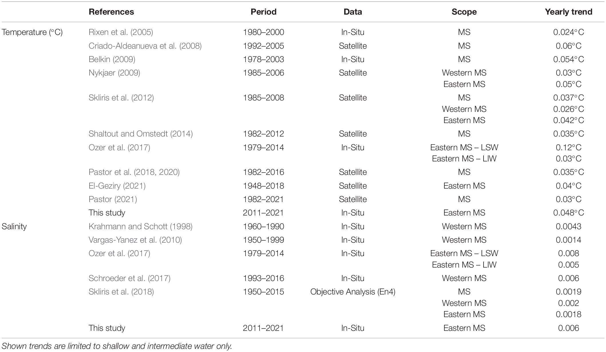
Table 1. Reported temperature and salinity yearly trends from investigations in various areas of the Mediterranean Sea, based on different data sources and time periods.

Tanhua et al. (2019) pointed out to the gaps in ocean observing coverage and the ever-growing use of the marine environment for both open ocean and coastal applications and the need to supply these users with operational services. Sustainable, long-term in situ monitoring programs are required for the improvement of coastal forecasts (Brenner et al., 2006), the calibration of remote sensing data and the enhancement of knowledge of the coastal water dynamics and their effects on the coastal ecological system. Pinardi and Coppini (2010) articulated: “The high variability of ocean currents and the need for the assessment of the state of the marine environment require a continuous monitoring of the ocean environment at unprecedented resolution and quality. On the other hand, scientific discoveries require continuous observations of the essential state variables of the system in order to detect new basic mechanisms and processes.”

In this study, we perform a comprehensive analysis of the thermohaline variability of regional coastal waters, in order to better characterize the coastal marine environment, its predominating temporal trends and their linkage with atmospheric forcing and advection. Using the time series of the Israeli coastal monitoring stations, unprecedented for this region in terms of temporal resolution, we investigate coastal variability and dynamics in the eastern MS, and elucidate on the issues of: (1) long term and inter annual trends, including a comparison to open ocean findings, (2) the predominance of the seasonal cycle, and (3) the connectivity of coastal waters along the Israeli coast.

Materials and Methods

The Israeli Coastal Monitoring Stations

In the framework of the National Monitoring Program of Israel’s Mediterranean waters (INMoP), Israel Oceanographic and Limnological Research (IOLR) operates two continuous observation posts with near-real-time data transfer to IOLR server¹. These stations are located at the westernmost edge of the coal terminals in Hadera (north) and Ashkelon (south), 2.2 kms offshore at water depths of 26 m (Figure 1). Hadera station (MedGloss # 80) was established toward the end of 1991, upgraded through the years and currently includes a bottom mounted, up looking, Teledyne RD Instruments 600 KHz Workhorse Monitor Waves ADCP located ∼100 m westward from the terminal end at water depth of 26 m. A Paroscientific Inc. Intelligent Digiquartz 8800 sea level sensor (PAROS) and a SBE16plusV2 Sea-Bird CTD (added to Hadera station in 2011) are installed on the westernmost terminal sporting pole at a depth of 11–12 m. The CTD is equipped with standard T/C duct and pressure sensors together with auxiliary sensors of dissolved oxygen (SBE63 Optode, Sea-Bird electronics) and fluorescence and turbidity sensors (FLNYU, WetLabs). A twin station at Ashkelon was established in mid-2012. Continuous CTD Raw data of T, S, Pressure, Oxygen, Fluorescence and Turbidity is collected at a high temporal sampling interval of 10 min. In order to ensure the systems durability against fouling it incorporates several antifouling measures including toxin emitting capsules, Bio-Wipers and an in-house developed underwater case minimizing the systems exposure to the surroundings. A routine maintenance procedure is preformed once every 2 months (for each of the stations) which includes the replacement of the CTD to a freshly authenticated instrument and the collection of reference measurements for data validation. Recovered CTDs go through a robust cleaning procedure (following Sea-Bird electronics guidelines) and are examined for biases both pre-cleaning (in comparison to the collected reference data) and post-cleaning in lab-performed comparisons. CTDs are sent to the manufacturer for calibration regularly every 2 years or earlier in the case of an identified drift of one of the sensors (i.e., over three times of the instruments initial accuracy of ±0.001°C for T and ±0.004 for S). The Hadera station CTD dataset encompasses the period of March 2011 to June 2021. Due to various infrastructure difficulties, Ashkelon station experienced large data breaks since its establishment in 2012. For this reason, Ashkelon CTD measurements will only be used here as a basis of comparison to Hadera station data.

FIGURE 1

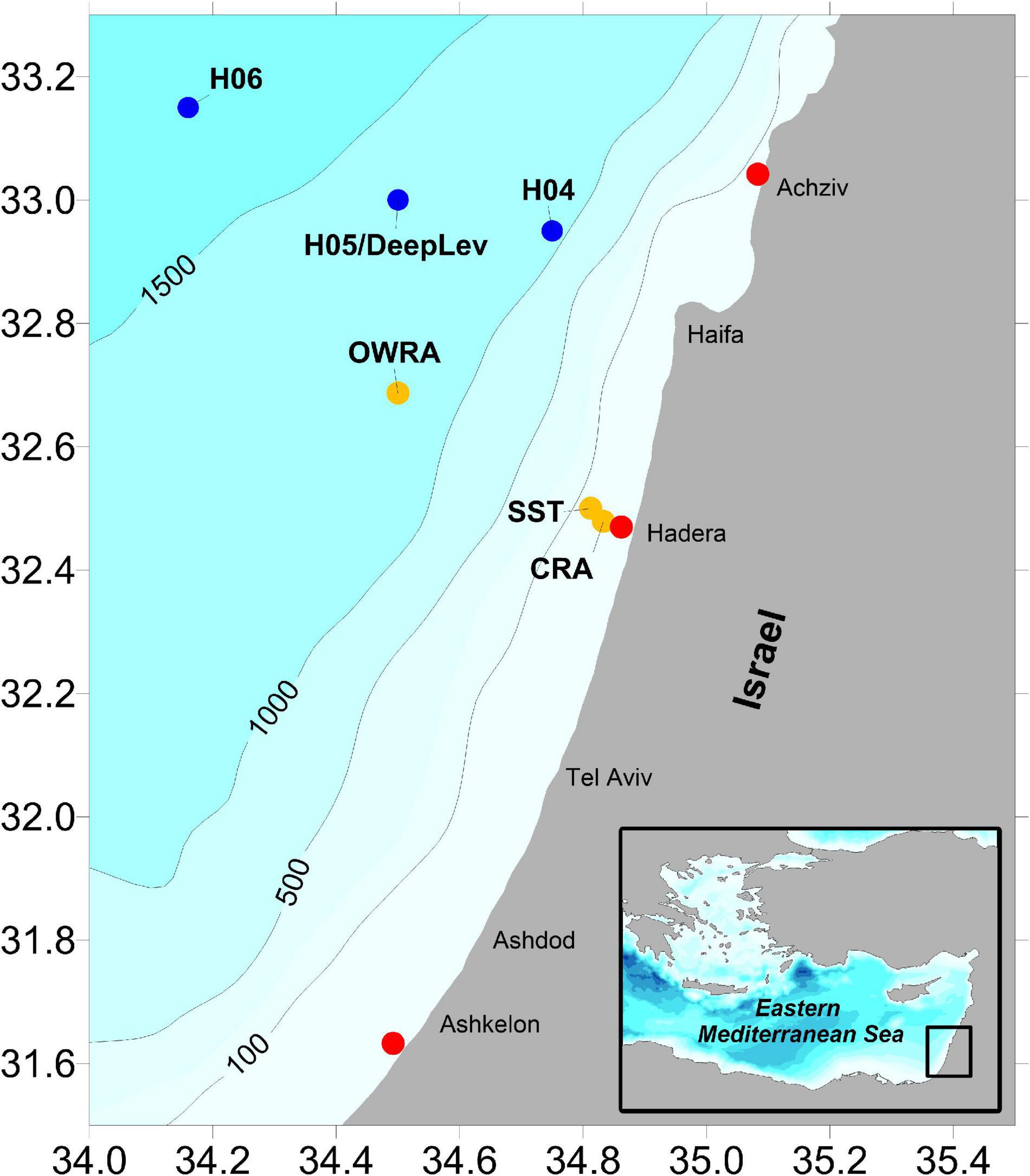
Figure 1. Spatial coverage of used datasets. Coastal stations locations (red). CMEMS reanalysis and SST positions (yellow). DeepLev and Haifa Section open water stations (blue).

Hadera station is located offshore (2.2 km) from the discharge of effluents at the shoreline of the nearby power plant and desalination facility. In order to assess the possible effect of these anthropogenic activities on our measurements, we examined the thermohaline marine monitoring report conducted in the area over the period of 2013 till 2020 (Cohen, 2021). T and S anomalies presented in the report, both for surface and near bottom values, are generally confined to a distance of ∼500 m from the shoreline and have a consistent southward spreading pathway, not effecting the station. Wood et al. (2020) used numerical simulations to study the distribution of desalination brines along the Israeli coast and the spreading of annual mean S anomalies in Hadera limited to under 1 km from the discharge location. To further confirm that Hadera monitoring station can be considered a good representative of northern Israeli coastal waters, a comparison of the daily averaged T time series to Achziv and SST datasets (see below) was performed. This comparison presented a statistically significant fit with a RMSE of 0.46 and Pearson R of 0.99 for the Achziv dataset and a RMSE = 0.66 and Pearson R of 0.98 for the SST dataset (Supplementary Figure 1).

Additional Data

Achziv Islands

Over a period of 13 months, from May 2013 to May 2014 Several HOBO T loggers were maintained at two sites in Achziv Islands, located at the northern end of the Israeli Mediterranean coast (Figure 1). The averaged data of two loggers deployed at a water depth of 10 m (north and south Islands, 1 and 1.3 km offshore) is used in comparison to the Hadera station dataset.

Haifa Section Cruises

Israel Oceanographic and Limnological Research conducts the biannual Haifa section cruise covering stations at water depths of 15–1900 m, extending 90 km off the coast of Israel, as a part of INMoP. A Sea-Bird SBE911plus CTD, interfaced to a SBE Carousel is used to collect continuous profiles of pressure, T, S, dissolved oxygen and fluorescence. Equipment, procedures, and calibrations are detailed in Ozer et al. (2017, 2019). We compare our results to the updated analysis of long-term and inter-annual trends as presented in Ozer et al. (2017) adding the years of 2015 to 2020.

Meteorology

Air T, wind, and precipitation data from four chosen stations in the vicinity of Hadera (Zikhron Ya’akov, Hadera port, Ein HaHoresh, and Ein Carmel) was averaged to attain a daily time series for the studied period of 2011 to 2021. The use of multiple stations covering ∼30 km along the Israeli coastal plain allowed to reduce data breaks, while maintaining the climatic traits of the region. All data originates from the Israel Meteorological Service (IMS) archive available online².

Copernicus Monitoring Environment Marine Service Data

We use two products provided by the E.U. Copernicus Monitoring Environment Marine Service (CMEMS). (1) Daily gap-free remotely sensed L4 SST produced and distributed in near-real time by the Consiglio Nazionale delle Ricerche (Buongiorno Nardelli et al., 2013). We extract the T time series from the high spatial resolution product (HR 0.0625°) in the closest position to Hadera station (32.5°N, 34.81°E). (2) The Mediterranean Sea Physical Reanalysis generated by a numerical system composed of a hydrodynamic model, supplied by the Nucleous for European Modeling of the Ocean and a variational data assimilation scheme (Escudier et al., 2020). Here we extract the daily time series of T and S for a depth of 10.5 m from two grid points of the reanalysis. The first representing coastal water closest to Hadera station (referred hereafter as CRA, 32.48°N, 34.83°E) and the second from an open water location (Z > 1200 m) northwest of Hadera station (referred hereafter as OWRA, 32.69°N, 34.5°E).

DeepLev Mooring Station

In November 2016, the first moored station at the Eastern LB was deployed at 1500m water depth, ∼50km offshore Haifa, Israel (Katz et al., 2020). For this study, we use the T time series from a downward looking Teledyne RD Instruments 300 KHz workhorse ADCP. The ADCP is installed on the upmost buoy of the mooring system, at a depth range of 20–30 m (depending on deployment) and sampling at a 15-min interval. The ADCP integrated T sensor has a reported precision of ±0.4°C and a resolution of 0.01°C. Inter-calibrations with CTD casts taken on deployment and recovery events yielded a mean variance of 0.015°C with a 95% confidence interval of ± 0.056°C (n = 11).

Data Analysis

At a preliminary stage the various time series data sets described above were aggregated into a unified database and synchronized based on the time of measurement. Next daily and monthly averages were calculated for all available parameters. T hourly averages grouped by month were attained to infer the range of the diurnal cycle (Supplementary Figures 2, 3). In addition, daily standard deviation averages of the complete CTD dataset (over 400,000 measurements in total) were calculated and yielded 0.19°C and 0.032 for T and S, respectively. The seasonal Mann-Kendall test was used to examine the T and S CTD datasets for statistically significant long-term trends (Hirsch et al., 1982; Hussain and Mahmud, 2019).

Ekman Transport Calculation

To ensure that the IMS wind dataset adequately represents off shore conditions, the daily averaged wind was compared with a time series of the ECMWF ERA-5 reanalysis at position 32.5°N, 34.75°E and presented a strong agreement with R² of 0.85 and 0.87 for U and V components, respectively (not shown). Next, following Cropper et al. (2014) across and along shore wind stress (τ) components were derived from averaged daily wind speeds.

${\mathrm{\tau }}_{ac}={\rho }_a{C}_d{\left(W_{ac}^2+W_{al}^2\right)}^{1/2}{W}_{ac}and$

${\mathrm{\tau }}_{al}={\rho }_a{C}_d{\left(W_{ac}^2+W_{al}^2\right)}^{1/2}{W}_{al}$

where, W_ac and W_al are across and along shore winds components achieved by a 25° rotation of the original data, according to the shoreline inclination. ρ_a is the air density of 1.22 kg/m³ and C_d the typical dimensionless drag coefficient of 1.3 × 10^–3. Next Ekman transport (Q) components were derived from the wind stress field.

$Q_{ac}=\frac{{\mathrm{\tau }}_{al}}{{\rho }_{w}f}and{Q}_{al}=\frac{-{\mathrm{\tau }}_{ac}}{{\rho }_{w}f}$

where, ρ_w is the density of sea water of 1025 kg/m³ and f is the Coriolis parameter defined as f = 2Ω sin(φ) (where, Ω is the earths angular velocity of 7.292 × 10^–5 s^–1 and φ is the latitude).

Filling Temperature Data Gaps

In order to complete missing CTD T data in the Hadera dataset a multi parameter regression (MPR) was performed. The MPR procedure was based on T records of the ADCP and PAROS, located in the immediate vicinity of the CTD, as well as the close by (∼1.3 km) SST dataset (Supplementary Figure 4). As a preliminary step the similarity of these datasets was assessed where they overlapped. Daily differences between the CTD T and the additional T datasets were computed and yielded 95% confidence intervals of 0.024, 0.016 and 0.028°C for ADCP, PAROS and SST, respectively. Pearson R correlation ranged from 0.97 to 0.99 (the lowest found between the ADCP and SST), thus all datasets were accepted for the MPR procedure. Depending on the availability of data from these datasets a matrix of coefficients was calculated and used to achieve a complete daily data set of Hadera station over the period of March 01, 2011 to June 08, 2021 (Supplementary Tables 1, 2). This method was not implemented for Ashkelon station as the data gaps there were considered too large to overcome. In the analysis of S variations, the monthly averaged data set was used, as no other reference was available in order to complete missing daily data.

Time Series Decomposition

For the determination of seasonal, trend and irregular components we follow Pezzulli et al. (2005) and use the filter based X11-ARIMA method (X11), a variant of the Census Method II Seasonal Adjustment Program, assuming an additive model.

$X_t=T_t+S_t+I_t$

where, X_t is the original time series, T_t is the trend component, S_t is the net seasonal component and I_t is the irregular variation. The X11 is a filter based method for seasonal adjustment which follows the ‘ratio to moving average’ procedure first described by Macaulay (1931) and commonly referred to as “Classical Decomposition.” In principle X11 is comprised of three steps which are implemented iteratively: (1) Estimation of the trend by a moving average, (2) Removal of the trend from the time series leaving the seasonal and irregular components, and (3) Estimation of the seasonal component using moving averages to smooth out the irregulars. After three iterations, the irregular term is finally calculated by removing the final trend and seasonal terms from the original time series. Key features of the X11 decomposition are that the trend is void of the annual cycle and any higher frequencies and that the seasonal term is defined locally in time, thus allowing for inter-annual variations in the seasonal cycle (Pezzulli et al., 2005). For the T decomposition, we use the daily averaged T and apply the moving averages windows of 30 × 365 and 30 × 30 for the trend and seasonal estimations, respectively. Due to the data gaps in the daily S dataset (Figure 2E), we implement the X11 decomposition on monthly averaged S and apply the moving averages windows of 2 × 12 and 2 × 2 for the trend and seasonal estimations, respectively. Similarly, the X11 method was also implemented on the daily CMEMS model reanalysis datasets (CRA and OWRA) in order to compare of the trend terms.

FIGURE 2

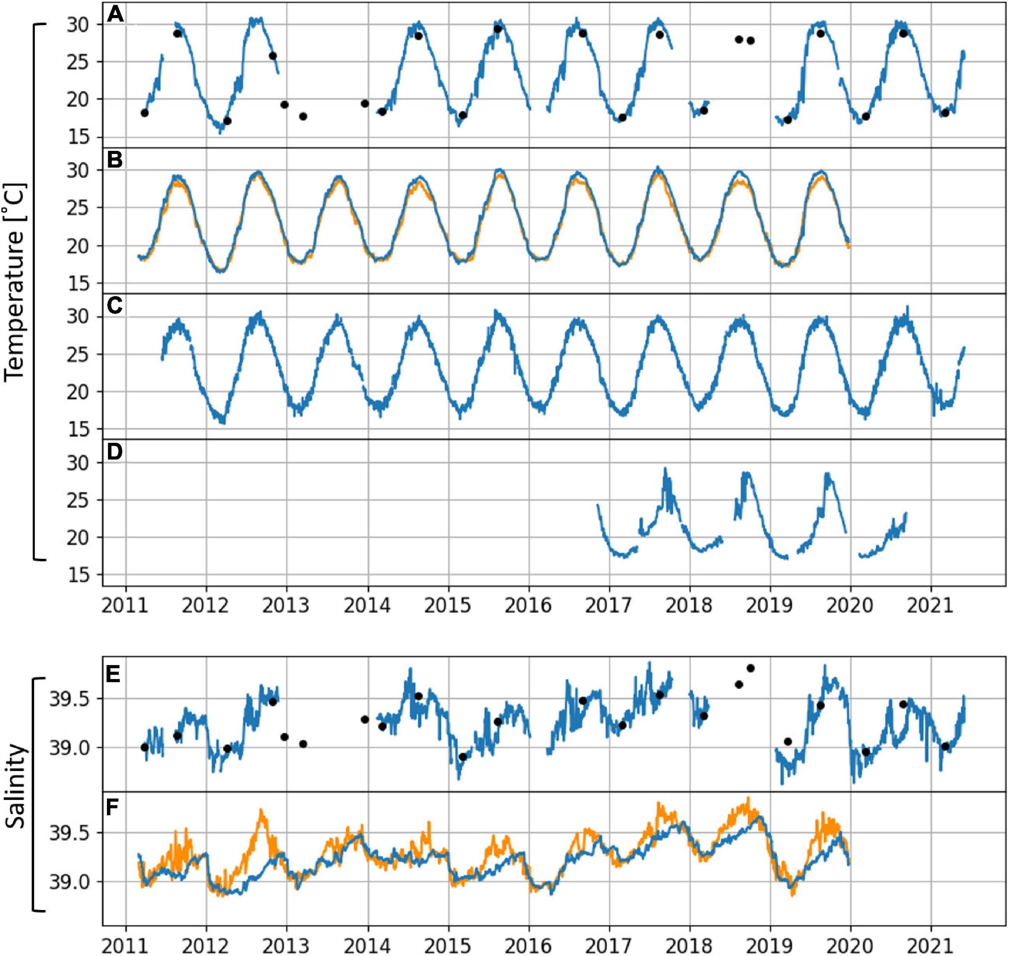
Figure 2. Temperature [A: Hadera CTD, B: CMEMS reanalysis CRA (blue) and OWRA (orange), C: SST, and D: DeepLev] and salinity [E: Hadera CTD and F: CMEMS reanalysis CRA (blue) and OWRA (orange) time series used for lag correlations and additional analysis]. Haifa section open water stations averaged surface values (upper 20 m) in black dots (A,E).

Synoptical Anomalies Delineation

The daily T irregular term (acquired by means of the X11 method) was further investigated by applying a threshold filter, parsing through this dataset and marking positive and negative amplitudes and durations. In order to set the thresholds for significant synoptical anomalies, we initially examined the amplitude of the diurnal cycle, which ranged from 0.15°C in winter to 0.3°C in summer for T (Supplementary Figure 2) and from 0.001 in winter to 0.003 in summer for S (Supplementary Figure 3). Since the S diurnal amplitude was at the level of sensor accuracy, we opted to use the values of ±2 times the average daily standard deviation (0.38°C for T and 0.064 for S) for the anomalies delineation. In every incident that the irregular term crossed the threshold value, the duration of the anomaly was recorded together with the maximal amplitude. Cases of missing data whilst within a given anomaly event were omitted as the anomaly period could not be established. For the S time series, where the X11 method was performed on monthly averages, the following approach was used to calculate daily anomalies. The interpolated sum of trend and seasonal terms (of the monthly X11 analysis) were subtracted from daily averaged CTD data where it was available. The resulting residuals time series was then screened following the same procedure described above for T.

Results and Discussion

Long-Term Trends and Inter-Annual Fluctuations

A statistically significant warming trend was identified over the observed period (2011–2021) in Hadera station (11–12 m depth) using the seasonal Mann-Kendall test, with a yearly rate of 0.048°C (p = 0, z = 10.92) (Figure 3A). While the coastal dataset has the handicap of covering a relatively short period of time, the achieved trend is in agreement with previous studies (Table 1), specifically it is very similar to the trends found in investigations of the eastern MS (Nykjaer, 2009; Skliris et al., 2012; El-Geziry, 2021), all yielding exceptionally high values. When compared to the trends obtained from open water casts offshore the Israeli coast (Ozer et al., 2017, updated analysis covering the years 1979–2020 in Supplementary Figure 5), the Hadera trend is similar to that achieved in the analysis of Levantine Intermediate Water (LIW) (0.03 ± 0.01°C year^–1), yet lower than the trend observed in surface water (0.13 ± 0.05°C year^–1). We attribute the disparity between Hadera and LSW trends to the fact that the analysis of LSW was limited to casts performed during the peak of the warming period (end of summer). In contrary, the analysis of LIW was based on bi-annual data (i.e., summer and winter casts). Furthermore, we consider the LIW to be less affected by mesoscale and seasonal processes, thus it is more integrative and reflective of long-term and inter-annual variability.

FIGURE 3

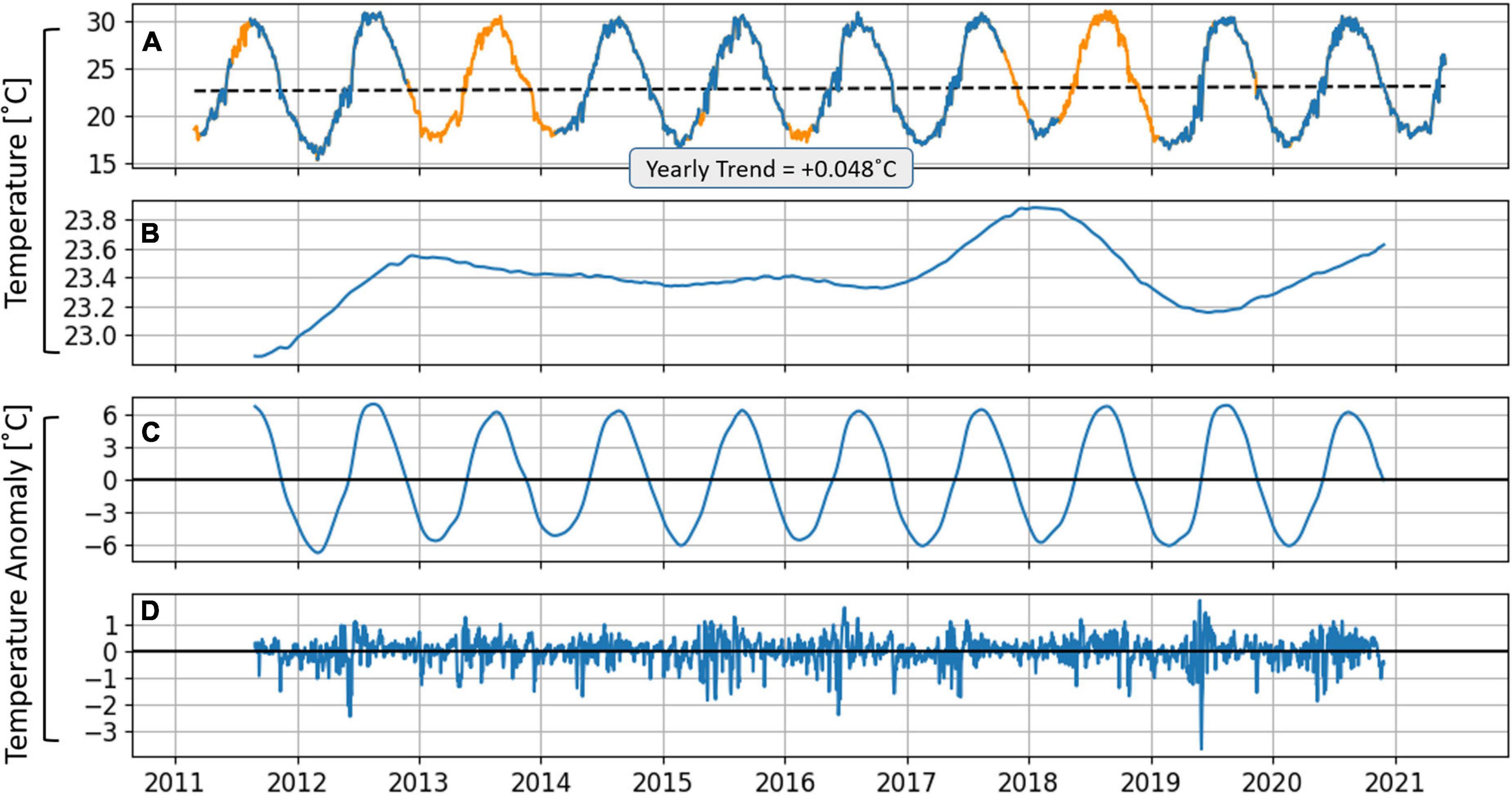
Figure 3. Daily averaged surface water temperature (A) – Hadera CTD values (blue) and missing data completed using multi parameter regression (orange). Calculated trend (B), seasonal (C), and irregular (D) terms achieved using the X11 decomposition method. Yearly linear trend accepted with the seasonal Mann-Kendall test of 0.048°C (p = 0, z = 10.92) presented in panel (A) (dashed black line and text box).

A significant positive S yearly trend of 0.006 (p = 4.06 × 10^–7, z = 5.06) was identified in the Hadera CTD dataset (Figure 4A). This trend is at the higher end of previously published salinification rates for the MS (Table 1), similar to the rates attained in the analysis of LSW and LIW (Ozer et al., 2017 and Supplementary Figure 5) and in the western MS (Schroeder et al., 2017). Pastor et al. (2018) reported upper layer salinification trends exceeding 0.004 year^–1 in the easternmost MS, in agreement with our results. This trend is consistent with the increase in latent heat loss in the eastern MS since the early 1970s (Mariotti, 2010; Skliris et al., 2012) and the large reduction in Nile river runoff since the early1960s (Skliris and Lascaratos, 2004; Suari and Brenner, 2015). The short duration of the dataset analyzed in this study does not support the appraisal of our findings within a broader framework of surface T and S natural variability of longer decadal and multi-decadal scales. These will need to be addressed in the future, as data accumulates from the coastal stations.

FIGURE 4

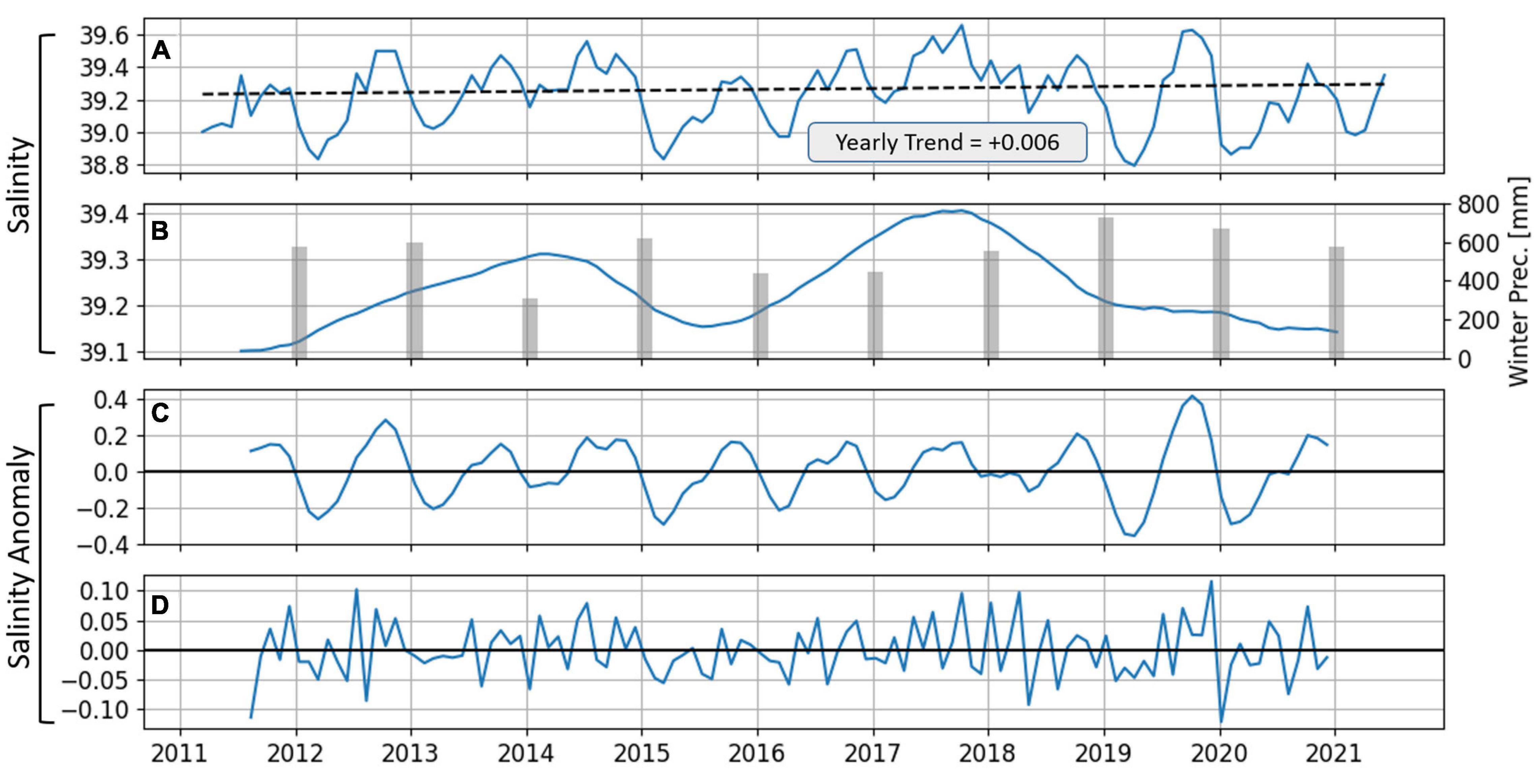
Figure 4. Monthly averaged Hadera CTD salinity values (A). Calculated trend (B), seasonal (C), and irregular (D) terms achieved using the X11 decomposition method. Yearly linear trend accepted with the seasonal Mann-Kendall test of 0.006 (p = 4.06 × 10^{– 7}, z = 5.06) presented in Panel A (dashed black line and text box). Total winter precipitation is superimposed on the trend in Panel B (Gray bars).

Both T and S trends achieved through the X11 method show inter-annual fluctuation with a clear maximum in the beginning of 2018, which seemingly corresponds with the previously established inter-annual cycle of the Levantine basin in connection with the BiOS mechanism (Civitarese et al., 2010a,b; Gacic et al., 2010; Ozer et al., 2017). Smaller, less prominent extremes are evident at the start of 2013 for T and 1 year later for S (Figures 3B, 4B). A close similarity is found between the T and S X11 trend terms of Hadera and CMEMS reanalysis datasets (Figure 5). The T Trends of Hadera and CRA are consistently higher than that of the OWRA, displaying the stronger response and higher sensitivity of coastal waters to the atmospheric forcing and their potential impact on the marine environment (Figure 5A). The S extrema of 2014 coincides with low precipitation in the winter of 2013–2014 (Figure 4B). Indeed, a correspondence of the coastal S seasonal minimum to the total winter precipitation can be observed throughout the examined period. To demonstrate the influence of precipitation on coastal S, we calculate the regression between S and cumulative precipitation in two winters seasons (covering the months of November to March) where salinity measurements were rarely interrupted. A strong relation is found with R² of 0.9324 and 0.885 for the winters of 2014–2015 and 2019–2020, respectively. On several occasions, drops of S values below the regression line are supported by a passing winter storm with several days of continuous high precipitation levels (Figure 6). These results point to a strong linkage of the surface S with the local rainfall. As S trends of CRA and OWRA follow the same temporal patterns (Figure 5B) we believe this is a close representation of the response to annual changes in the LB regional water budget.

FIGURE 5

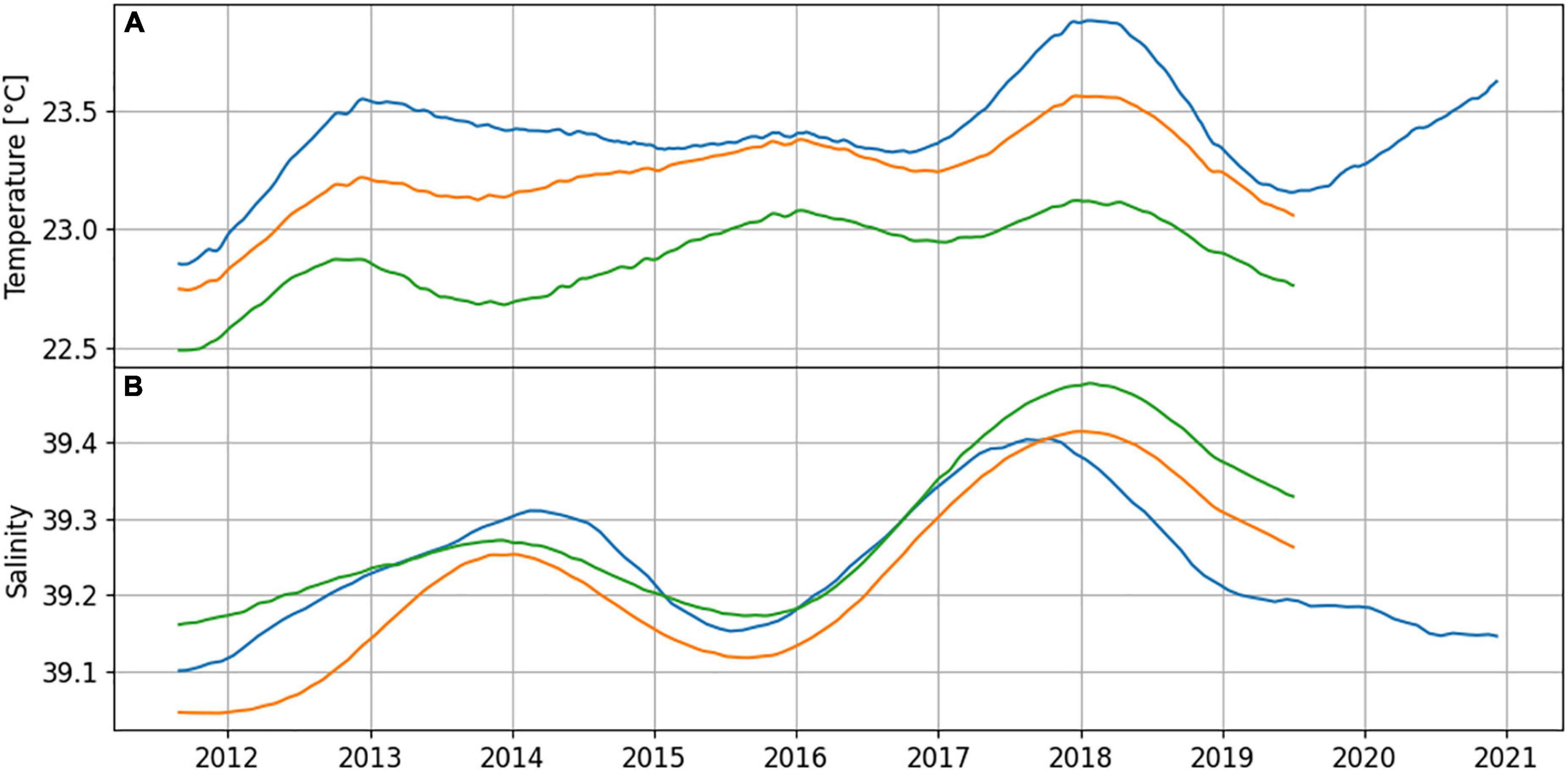
Figure 5. Temperature (A) and Salinity (B) trend terms achieved using the X11 decomposition method on daily data for the Hadera CTD dataset (blue, as shown in Figures 3, 4), CMEMS model reanalysis close to Hadera station (i.e., CRA and orange) and CMEMS model reanalysis at open water location (i.e., OWRA and green).

FIGURE 6

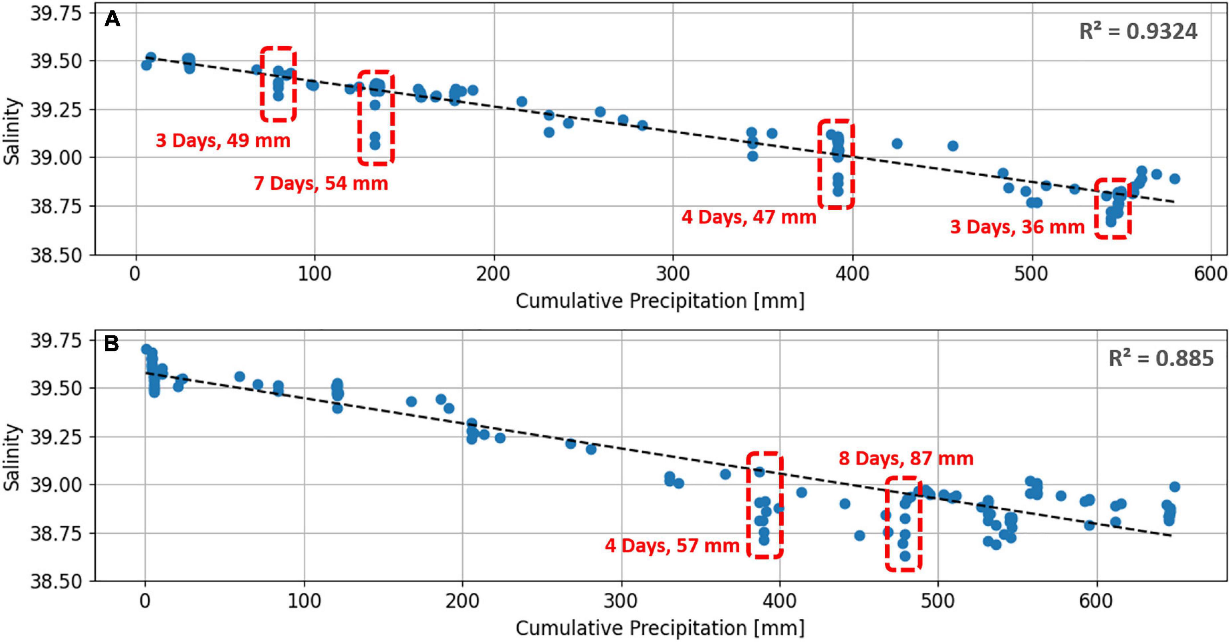
Figure 6. Salinity measurements from Hadera monitoring station projected against winter cumulative precipitation for the winters of 2014–2015 (A) and 2019–2020 (B). Calculated regression line are shown in dashed black lines (identical for both winter seasons, y = –0.0013x + 39.55). Red rectangles and adjoining text indicate storms where high precipitation levels were recorded coinciding with a salinity drop below the regression line. Storms duration and total precipitation are indicated in red text.

The overall agreement of T and S time series of the OWRA with Hadera station in terms of variance and lags (Table 2), as well as the similarities of the T and S X11 trends discussed above, indicates a relatively strong coupling between coastal water and the open ocean. In contrast, a large difference is found between T time series of Hadera and DeepLev mooring with a time lag of 43 days (Table 2). We attribute this inconsistency of DeepLev data to the fact that the T in this dataset is sampled at a deeper level (∼30 m), below the surface mixed layer in summer, thus the changing level of the vertical mixing has a significant effect on the sampled data.

TABLE 2

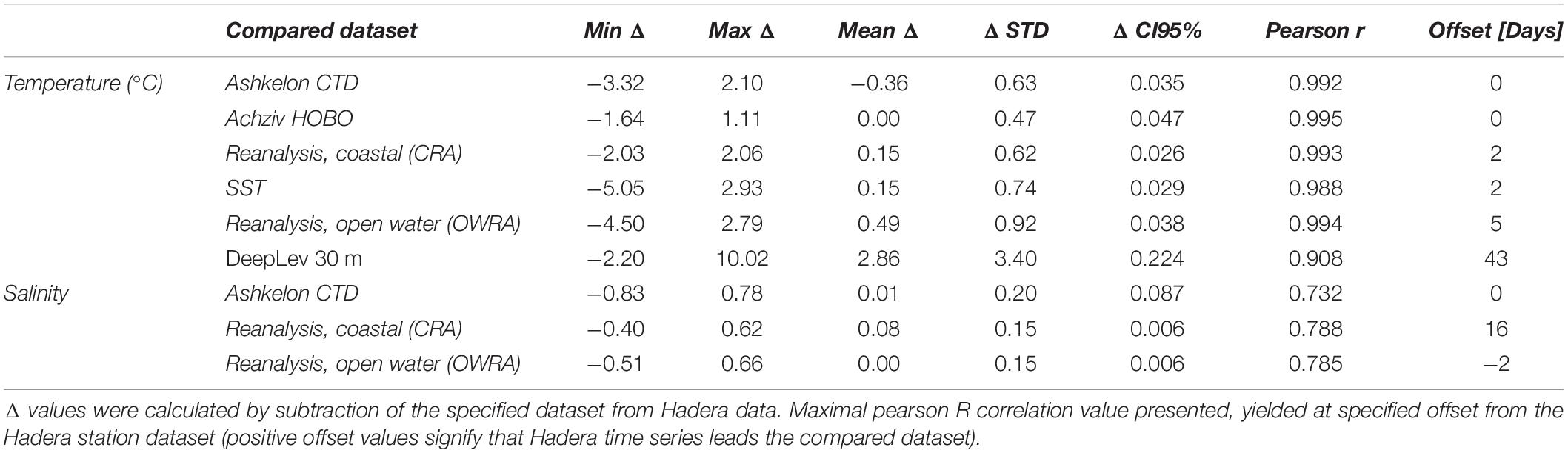
Table 2. Summary values for temperature and salinity contemporaneous datasets compared with Hadera station time series.

Climatology and the Seasonal Cycle

A clear seasonal cycle of surface T is evident in our data with average peak values of 29.86°C in August and 17.62°C in February, representing an average offset of +7°C in summer and −5°C in winter from the overlaying long-term trend (Figures 7A, 3B,C). Extreme water T seasonal anomalies are in concordance with large amount of days with air T below 10°C for negative anomalies and above 25°C for positive anomalies (not shown). Lag correlations performed between the average daily air T and CTD thermohaline values confirms the expected seasonal effect of atmospheric forcing on coastal water characteristics, with the air T time series leading by 15 and 50 days before water T and S, respectively (Supplementary Figure 6). The S dataset presents a less coherent seasonal sequence with a bimodal behavior in the summer seasons of 2014, 2016, and 2017, which is apparent also in the climatological S (Figures 4C, 7B). The drop in salinity in August can be attributed to the intensification of the along shore current in the period of June-July (Figure 7C), potentially advecting more AW which are lower in their S value. Wind derived along shore Ekman transport is kept close to zero in the summer months (Figure 7D), suggesting that the strong current values are mainly of geostrophic origin. Rosentraub and Brenner (2007) reported maximal northward currents in the summer season over the Israeli continental shelf confined to the upper layer as well as an along-slope baroclinic jet during summer and early winter. The authors related their findings to the general surface circulation of the LB introducing AW into the basin through several established pathways. Mauri et al. (2019) has shown an increase in average dynamic topography during the months of June to August in latitudes of 33–34 N in further support of our hypothesis. Estournel et al. (2021) demonstrated that in summer, the shallower current flows closer to the coastline while in winter it flows above the 1000 m isobath. The climatological extrema S values of 39.47 and 39.01 are reached at the months of October and March, respectively. An extreme seasonal cycle is observed in 2019 with minimal S of 38.8, which we relate to the high precipitation of the preceding winter as discussed earlier. However, this minimum can also be related to an enhanced modified AW flux into the LB, following the reasoning of the BiOS mechanism. An unusual fast recovery brings S as high as 39.63 by October 2019 and is not supported by the meteorological datasets.

FIGURE 7

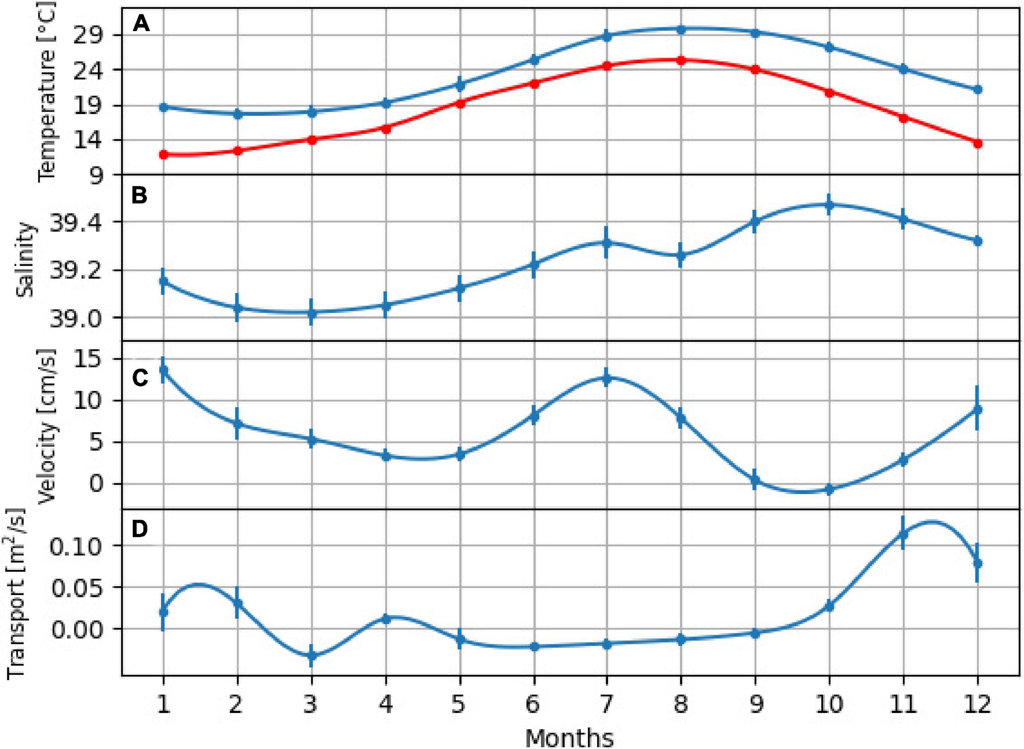
Figure 7. Climatological water temperature (A, blue), air temperature (A, red), salinity (B), along shore current component (C), and along shore Ekman transport (D). Standard error of averages shown in Vertical bars.

Synoptical Anomalies Analysis

T anomaly amplitudes range from +2 to −2.5°C with modal values reached at −0.67°C and 0.69°C for negative and positive anomalies, respectively (Figure 8A). The range of T anomalies duration is between 0 and 16 days with a maximal Kernel density at 1.5 days (Figure 8B). Similar anomaly behavior is observed for S, with a slight preference to negative anomalies and modal Kernel densities at −0.141 and 0.136 for negative and positive anomalies, respectively (Figures 8D,E). Averaged T anomaly amplitudes grouped by durations show a relation between the duration of the anomaly and its corresponding amplitude, the longer the anomaly lasts, the higher the amplitude. This apparent dependency is kept for both positive and negative anomalies, but is more coherent in the case of the latter. A similar, yet less clear relation can be observed for S. For both parameters, the majority of anomaly events last up to 10 days (Figures 8C,F). No significant seasonal T and S anomalies were identified (Supplementary Figure 7). We additionally perform an analysis of heat waves following the definition of the IPCC, 2019: “marine heatwaves are defined when the daily sea surface temperature exceeds the local 99th percentile over the period 1982 to 2016.” The 99th T percentile for the period of measurements in Hadera was calculated, resulting in 30.56°C. Running this filter brings up several heat waves (Supplementary Table 3) with somewhat higher maximum T toward 2018, yet our dataset is too short to identify any patterns.

FIGURE 8

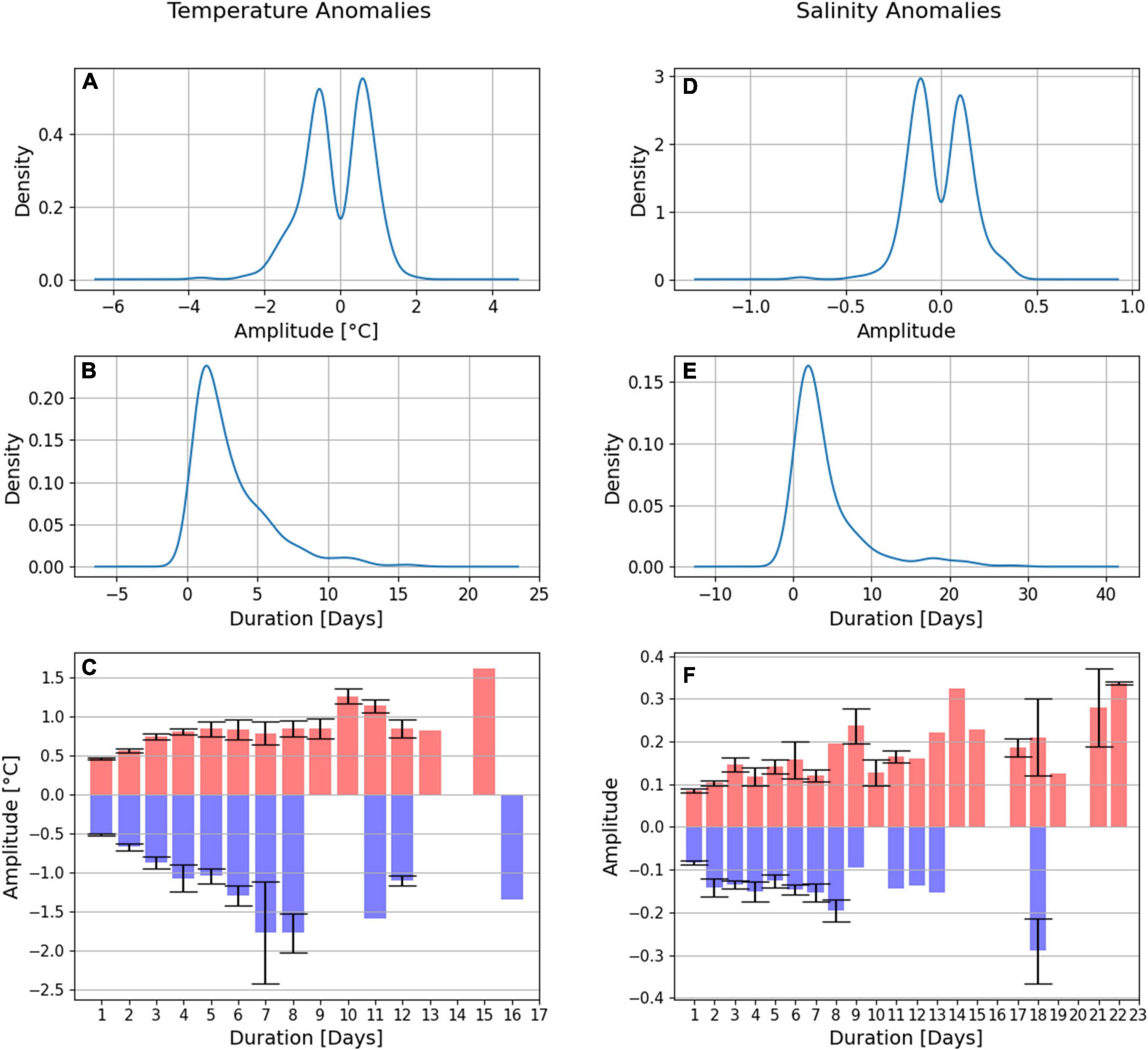
Figure 8. Kernel density estimation of amplitudes (A,D) and durations (B,E) for anomalies of temperature and salinity, respectively. Averaged temperature (C) and salinity (F) amplitudes of positive (red) and negative (blue) anomalies grouped by their duration. Standard error bars are shown where anomalies of a specific duration occurred more than once.

Along-Shore Connectivity

Variance statistics and lag correlations calculated for T and S comparing the Hadera station data to available datasets (Figure 2) are presented in Table 2. No offsets were found between the 3 stations (Hadera, Ashkelon and Achziv) demonstrating that the 180 km strip of Israeli coastal waters undergo seasonal and inter-annual changes in synchrony. Ashkelon station was found to be 0.36°C warmer than Hadera station, a fact we relate to its southerly location (100 km south of Hadera station) and to extended continental shelf at the south of Israel (over 20 km in width). A convincing relation was found between the positive T irregular term (from the X11 analysis) and the along shore currents, where the majority of T irregular values are explained by northward currents, the higher the T anomaly, the stronger the current (Figure 9A). A zero time offset yielded a maximal correlation between the irregular T and along shore currents (Figure 9B). These results suggest that the majority of positive T anomalies are a result of northward transport of water along the Israeli continental shelf, advecting warmer water from the south. No T gradient was found between Hadera and Achziv (distanced ∼70 km, Table 2), perhaps signifying that the northern shallow waters of Israel share a stronger connection maintained by coastal dynamics. T comparisons of CRA and Hadera T data yielded similar results with a mean difference of 0.15°C, high correlations and an offset of 2 days. The CRA S was found to be in average 0.08 below Hadera station. As both CRA and SST datasets are originated from westerly, deeper positions (compared with Hadera station), we infer that atmospheric forcing is enhanced at shallower, more easterly positions and is communicated toward the west over the continental shelf within synoptical timeframe. The large offset of S, where Hadera leads the CRA by 16 days remains unclear. No significant variance in S was found between Hadera and Ashkelon stations (Table 2).

FIGURE 9

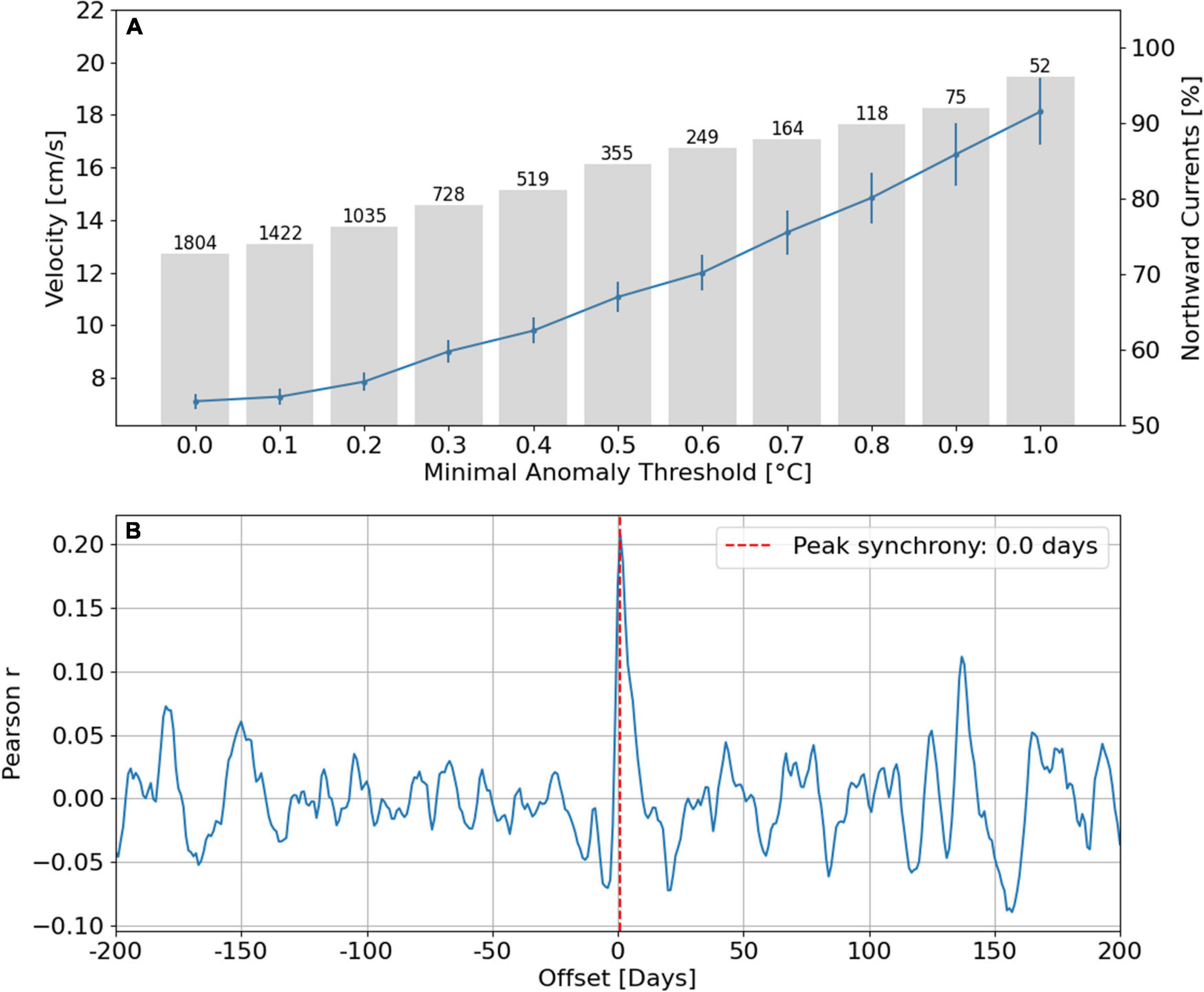
Figure 9. Correspondence between along shore currents and positive temperature anomalies. (A) The along shore current time series is filtered for increasing positive temperature anomaly thresholds (shown in the X axis). The resulting filtered along shore current dataset is averaged (blue line, vertical bars show standard error) and the percentage of incidents where northward currents coincide with the positive temperature anomaly is calculated (gray bars, total number of data points above the temperature threshold). (B) Lag correlation between temperature and along shore current residuals time series. Peak synchrony marked by red dashed line.

Conclusion

The continued study of coastal ocean state, variability, health and climate change through environmental monitoring programs plays an important role in broadening our knowledge and understanding of the changing seas, raises the public awareness, informs policy makers and supports the management of the coastal areas. The importance of sustained ocean and coastal observation, aimed at advancing our knowledge of the ocean and its link with climate, promoting the development of early warning systems, and enabling decision-making based on the best available science has become a global consensus (Tanhua et al., 2019). In this study we make use of continuous observations providing exclusive high temporal resolution data in the Eastern coast of the LB and address the issues of (1) long term and inter annual trends, (2) the coastal seasonal cycle, and (3) The connectivity of coastal waters along the Israeli coast. Significant long-term positive trends of T and S are validated by use of the seasonal Mann-Kendall test and compared to previously published findings in other areas of the MS. The T trend of 0.048°C identified in this study supports the exceptionally high warming rates reported in the eastern MS (Nykjaer, 2009; Skliris et al., 2012; El-Geziry, 2021) (Table 1). Filter based time series decomposition allows the identification of inter-annual T and S fluctuations associated with previously published open ocean dynamics (Ozer et al., 2017) as well as with CMEMS physical model reanalysis. Our results of higher coastal T trend term (Figure 5A), the impact of local winter rainfall on S values (Figure 6), and the sensitivity of T anomalies to the prevailing northward alongshore current (Figure 9) demonstrate the faster response time and higher sensitivity of the coastal environment to atmospheric forcing. Nonetheless, we infer a relatively strong coupling between coastal water and the open ocean in terms of long-term, inter-annual and seasonal evolution of the surface thermohaline properties. Finally, we stress the importance of the persistence of these monitoring efforts and the introduction of additional sustainable coastal waters stations, which will improve the spatial coverage enabling a better interpretation and understanding of the predominating processes.

Data Availability Statement

The datasets presented in this study can be found in online repositories. The names of the repository/repositories and accession number(s) can be found below: Israel Marine Data Center – https://isramar.ocean.org.il/isramar2009/.

Author Contributions

TO led manuscript drafting with the help of BH, IG, and HG. TO and IG contributed to the data acquiring. HG and BH contributed to the interpretation. All authors approved the submitted version.

Funding

This study was supported by the Israel Ministries of Energy and Environmental Protection through the National Monitoring Program of Israel’s Mediterranean waters. This study is in fulfillment of a Ph.D. thesis of Tal Ozer at the University of Haifa.

Conflict of Interest

The authors declare that the research was conducted in the absence of any commercial or financial relationships that could be construed as a potential conflict of interest.

Publisher’s Note

All claims expressed in this article are solely those of the authors and do not necessarily represent those of their affiliated organizations, or those of the publisher, the editors and the reviewers. Any product that may be evaluated in this article, or claim that may be made by its manufacturer, is not guaranteed or endorsed by the publisher.

Acknowledgments

We thank the Maritime Crew, Electrical Lab, and Research Assistants at the Physical Oceanography Department at IOLR for their continued and dedicated efforts on the routine service and maintenance of the Hadera and Ashkelon monitoring stations. We additionally thank the crew of the R.V. Bat Galim and the former IOLR R.V. Shikmona for their contribution and support to the Haifa section and DeepLev mooring cruises.

Supplementary Material

The Supplementary Material for this article can be found online at: https://www.frontiersin.org/articles/10.3389/fmars.2021.799457/full#supplementary-material

Footnotes

1. ^ https://isramar.ocean.org.il
2. ^ https://ims.data.gov.il/ims/7

References

Amitai, Y., and Gildor, H. (2016). Can precipitation over Israel be predicted from Eastern Mediterranean heat content? Int. J. Climatol. 37, 2492–2501.

Google Scholar

Belkin, M. (2009). Rapid warming of large marine ecosystems. Prog. Oceanogr. 81, 207–213. doi: 10.1016/j.pocean.2009.04.011

CrossRef Full Text | Google Scholar

Bindoff, N. L., Cheung, W. W. L., Kairo, J. G., Arístegui, J., Guinder, V. A., Hallberg, R., et al. (2019). “Changing ocean, marine ecosystems, and dependent communities,” in IPCC Special Report on the Ocean and Cryosphere in a Changing Climate, eds H.-O. Pörtner, D. C. Roberts, V. Masson-Delmotte, P. Zhai, M. Tignor, E. Poloczanska, et al. (Geneva: IPCC).

Google Scholar

Brenner, S., Murashkovsky, A., and Gertman, I. (2006). Assessment of one year of high-resolution operational forecasts for the Southeastern Mediterranean shelf region in the MFSTEP project. Ocean Sci. Discuss. 3, 2059–2085.

Google Scholar

Buongiorno Nardelli, B., Tronconi, C., Pisano, A., and Santoleri, R. (2013). High and ultra-high resolution processing of satellite sea surface temperature data over southern european seas in the framework of myocean project. Remote Sens. Environ. 129, 1–16.

Google Scholar

Civitarese, G., Gacic, M., Cardin, V., Borzelli, G. L. E., and Spa, T. (2010a). Effects of the adriatic-ionian bimodal oscillating system (Bios) on the biogeochemistry of the Adriatic Sea. CIESM Org. 28:2010.

Google Scholar

Civitarese, G., Gaèiæ, M., Lipizer, M., and Eusebi Borzelli, G. L. (2010b). On the impact of the bimodal oscillating system (BiOS) on the biogeochemistry and biology of the Adriatic and Ionian Seas (Eastern Mediterranean). Biogeosciences 7, 3987–3997. doi: 10.5194/bg-7-3987-2010

CrossRef Full Text | Google Scholar

Cohen, Y. (2021). Marine Monitoring by the Israeli Electric Company and H2ID Desalination Plant. RELP- 1 – 2021. Hadera: Israeli Electric Company.

Google Scholar

Collins, M., Knutti, R., Arblaster, J., Dufresne, J. L., Fichefet, T., Friedlingstein, P., et al. (2013). “Long-term climate change: projections, commitments and irreversibility,” in Climate Change 2013: The Physical Science Basis. Contribution of Working Group I to the Fifth Assessment Report of the Intergovernmental Panel on Climate Change, ed. IPCC (Cambridge: Cambridge University Press).

Google Scholar

Collins, M., Sutherland, M., Bouwer, L., Cheong, S. M., Frölicher, T., Jacot Des Combes, H., et al. (2019). “Extremes, abrupt changes and managing risk,” in IPCC Special Report on the Ocean and Cryosphere in a Changing Climate, eds H.-O. Pörtner, D. C. Roberts, V. Masson-Delmotte, P. Zhai, M. Tignor, E. Poloczanska, et al. (Geneva: IPCC).

Google Scholar

Criado-Aldeanueva, F., Del Río Vera, J., and García-Lafuente, J. (2008). Steric and mass-induced Mediterranean sea level trends from 14 Years of altimetry data. Glob. Planet. Change 60, 563–575.

Google Scholar

Cropper, T. E., Hanna, E., and Bigg, G. R. (2014). Spatial and temporal seasonal trends in coastal upwelling off Northwest Africa, 1981 – 2012. Deep Sea Res. Part I 86, 94–111. doi: 10.1016/j.dsr.2014.01.007

CrossRef Full Text | Google Scholar

Desbiolles, F., Alberti, M., Hamouda, M. E., Meroni, A. N., and Pasquero, C. (2021). Links between sea surface temperature structures, clouds and rainfall: study case of the Mediterranean Sea. Geophys. Res. Lett. 48:e2020GL091839.

Google Scholar

Efrati, S., Lehahn, Y., Rahav, E., Kress, N., Herut, B., Gertman, I., et al. (2013). Intrusion of coastal waters into the Pelagic Eastern Mediterranean: in situ and satellite-based characterization. Biogeosciences 10, 3349–3357.

Google Scholar

El-Geziry, T. (2021). Long-term changes in sea surface temperature (SST) within the Southern Levantine Basin. Acta Oceanol. Sin. Engl. Edn. 40, 1–7. doi: 10.5402/2013/392632

CrossRef Full Text | Google Scholar

Escudier, R., Clementi, E., Omar, M., Cipollone, A., Pistoia, J., Aydogdu, A., et al. (2020). Mediterranean Sea Physical Reanalysis (CMEMS MED-Currents) (Version 1) [Data Set]. Copernicus Monitoring Environment Marine Service (CMEMS). doi: 10.25423/CMCC/MEDSEA_MULTIYEAR_PHY_006_004_E3R1

CrossRef Full Text | Google Scholar

Estournel, C., Marsaleix, P., and Ulses, C. (2021). A new assessment of the circulation of Atlantic and intermediate waters in the Eastern Mediterranean. Prog. Oceanogr. 198:102673. doi: 10.1016/j.pocean.2021.102673

CrossRef Full Text | Google Scholar

Gacic, M., Eusebi Borzelli, G. L., Civitarese, G., Cardin, V., and Yari, S. (2010). Can internal processes sustain reversals of the ocean upper circulation? The Ionian Sea example. Geophys. Res. Lett. 37, 1–5.

Google Scholar

Gertman, I., and Hecht, A. (2002). Annual and long-term changes in the salinity and the temperature of the waters of the South-Eastern Levantine basin. CIESM 2002. Tracking long-term hydrological change in the Mediterranean Sea. Monaco, 22-24-April 2002. CIESM Workshop Ser. 16, 75–78.

Google Scholar

Giorgi, F. (2006). Climate change hot-spots. Geophys. Res. Lett. 33:L08707. doi: 10.1029/2006GL025734

CrossRef Full Text | Google Scholar

Giorgi, F., and Lionello, P. (2008). Climate change projections for the Mediterranean region. Glob. Planet. Change 63, 90–104. doi: 10.1016/j.gloplacha.2007.09.005

CrossRef Full Text | Google Scholar

Gissi, E., Manea, E., Mazaris, A. D., Fraschetti, S., Almpanidou, V., Bevilacqua, S., et al. (2021). A review of the combined effects of climate change and other local human stressors on the marine environment. Sci. Total Environ. 755:142564. doi: 10.1016/j.scitotenv.2020.142564

PubMed Abstract | CrossRef Full Text | Google Scholar

Hamad, N., Millot, C., and Taupier-Letage, I. (2005). A new hypothesis about the surface circulation in the Eastern Basin of the Mediterranean Sea. Prog. Oceanogr. 66, 287–298.

Google Scholar

Herut, B., Almogi-Labin, A. B., Jannink, N., and Gertman, I. (2000). The Seasonal dynamics of nutrient and chlorophyll a concentrations on the SE Mediterranean shelf-slope. Oceanol. Acta 23(7 SUPPL.), 771–782. doi: 10.1016/s0399-1784(00)01118-x

CrossRef Full Text | Google Scholar

Hirsch, R. M., Slack, J. R., and Smith, R. A. (1982). Techniques of trend analysis for monthly water quality data. Water Resour. Res. 18, 107–121. doi: 10.1029/WR018i001p00107

CrossRef Full Text | Google Scholar

Hussain, M. M., and Mahmud, I. (2019). pyMannKendall: a python package for non parametric Mann Kendall family of trend tests. J. Open Source Softw. 4: 1556. doi: 10.21105/joss.01556

CrossRef Full Text | Google Scholar

IPCC (2019). “Summary for policymakers,” in IPCC Special Report on the Ocean and Cryosphere in a Changing Climate, eds H.-O. Pörtner, D.C. Roberts, V. Masson-Delmotte, P. Zhai, M. Tignor, E. Poloczanska, et al. (Geneva: IPCC).

Google Scholar

IPCC (2021). “Climate change 2021: the physical science basis,” in Contribution of Working Group I to the Sixth Assessment Report of the Intergovernmental Panel on Climate Change, eds V. Masson-Delmotte, P. Zhai, A. Pirani, S. L. Connors, C. Péan, S. Berger, et al. (Cambridge: Cambridge University Press). doi: 10.1007/s10584-021-03233-7

PubMed Abstract | CrossRef Full Text | Google Scholar

Katz, T., Weinstein, Y., Alkalay, R., Biton, E., Toledo, Y., Lazar, A., et al. (2020). The first deep-sea mooring station in the eastern levantine basin (DeepLev), outline and insights into regional sedimentological processes. Deep Sea Res. Part II Top. Stud. Oceanogr. 171:104663. doi: 10.1016/j.dsr2.2019.104663

CrossRef Full Text | Google Scholar

Kirtman, B., Power, S. B., Adedoyin, J. A., Boer, G. J., Bojariu, R., Camilloni, I., et al. (2013). “Near-term climate change: projections and predictability,” in Climate Change 2013: The Physical Science Basis. Contribution of Working Group I to the Fifth Assessment Report of the Intergovernmental Panel on Climate Change, eds T. F. Stocker, D. Qin, G.-K. Plattner, M. Tignor, S. K. Allen, J. Boschung, et al. (Cambridge: Cambridge University Press).

Google Scholar

Krahmann, G., and Schott, F. (1998). Longterm increases in western Mediterranean salinities and temperatures: anthropogenic and climatic sources. Geophys. Res. Lett. 25, 4209–4212. doi: 10.1029/1998GL900143

CrossRef Full Text | Google Scholar

Kress, N., Gertman, I., and Herut, B. (2014). Temporal evolution of physical and chemical characteristics of the water column in the Easternmost levantine basin (Eastern Mediterranean Sea) from 2002 to 2010. J. Mar. Syst. 135, 6–13. doi: 10.1016/j.jmarsys.2013.11.016

CrossRef Full Text | Google Scholar

Lascaratos, A., Roether, W., Nittis, K., and Klein, B. (1999). Recent changes in deep water formation and spreading in the Eastern Mediterranean Sea: a review. Prog. Oceanogr. 44, 5–36. doi: 10.1016/s0079-6611(99)00019-1

CrossRef Full Text | Google Scholar

Ludwig, W., Dumont, E., Meybeck, M., and Heussner, S. (2009). River discharges of water and nutrients to the Mediterranean and Black Sea: major drivers for ecosystem changes during past and future decades? Prog. Oceanogr. 80, 199–217. doi: 10.1016/j.pocean.2009.02.001

CrossRef Full Text | Google Scholar

Macaulay, F. R. (1931). The smoothing of time series. By Frederick R. Macaulay. [Pp. 172. New York: national bureau of economic research, incorporated. 1931.]. J. Inst. Actuar. 62, 181–182. doi: 10.1017/s0020268100010003

CrossRef Full Text | Google Scholar

Malanotte-Rizzoli, P., Artale, V., Borzelli-Eusebi, G. L., Brenner, S., Crise, A., Gacic, M., et al. (2014). Physical forcing and physical/biochemical variability of the mediterranean sea: a review of unresolved issues and directions for future research. Ocean Sci. 10, 281–322.

Google Scholar

Mariotti, A. (2010). Recent changes in the Mediterranean water cycle: a pathway toward long-term regional hydroclimatic change? J. Clim. 23, 1513–1525. doi: 10.1175/2009JCLI3251.1

CrossRef Full Text | Google Scholar

Mariotti, A., Struglia, A., Struglia, M., Zeng, Y., Zeng, N., and Lau, K.-M. (2002). The hydrological cycle in the Mediterranean region and implications for the water budget of the Mediterranean Sea. J. Clim. 15, 1674–1690. doi: 10.1175/1520-4422002015<1674:THCITM<2.0.CO;2

CrossRef Full Text | Google Scholar

Mauri, E., Sitz, L., Gerin, R., Poulain, P. M., Hayes, D., and Gildor, H. (2019). On the variability of the circulation and water mass properties in the Eastern Levantine Sea between. Water 11:1741. doi: 10.3390/w11091741

CrossRef Full Text | Google Scholar

Micheli, F., Halpern, B. S., Walbridge, S., Ciriaco, S., Ferretti, F., Fraschetti, S., et al. (2013). Cumulative human impacts on mediterranean and black sea marine ecosystems: assessing current pressures and opportunities. PLoS One 8:e79889. doi: 10.1371/journal.pone.0079889

PubMed Abstract | CrossRef Full Text | Google Scholar

Miglietta, M., Moscatello, A., Conte, D., Mannarini, G., Lacorata, G., and Rotunno, R. (2011). Numerical analysis of a Mediterranean ‘hurricane’ over South-Eastern Italy: sensitivity experiments to sea surface temperature. Atmos. Res. 101, 412–426. doi: 10.1016/j.atmosres.2011.04.006

CrossRef Full Text | Google Scholar

Nykjaer, L. (2009). Mediterranean sea surface warming 1985–2006. Clim. Res. 39, 11–17.

Google Scholar

Ozer, T., Gertman, I., Gildor, H., Goldman, R., and Herut, B. (2019). Evidence for recent thermohaline variability and processes in the deep water of the Southeastern Levantine Basin, Mediterranean Sea. Deep Sea Res. Part II Top. Stud. Oceanogr. 171:104651. doi: 10.1016/j.dsr2.2019.104651

CrossRef Full Text | Google Scholar

Ozer, T., Gertman, I., Kress, N., Silverman, J., and Herut, B. (2017). Interannual thermohaline (1979–2014) and nutrient (2002–2014) dynamics in the levantine surface and intermediate water masses, SE Mediterranean Sea. Glob. Planet. Change 151, 60–67. doi: 10.1016/j.gloplacha.2016.04.001

CrossRef Full Text | Google Scholar

Pastor, F. (2021). Mediterranean Sea Surface Temperature Report (Spring 2021). Meteorology and Pollutant Dynamics Area. Valencia: The Mediterranean Center for Environmental Studies (CEAM). doi: 10.13140/RG.2.2.15757.05600

CrossRef Full Text | Google Scholar

Pastor, F., Valiente, J. A., and Estrela, M. J. (2015). Sea surface temperature and torrential rains in the valencia region: model ling the role of recharge areas. Nat. Hazards Earth Syst. Sci. 15, 1677–1693.

Google Scholar

Pastor, F., Valiente, J. A., and Khodayar, S. (2020). A Warming Mediterranean: 38 years of increasing sea surface temperature. Remote Sens. 12:2687. doi: 10.3390/rs12172687

CrossRef Full Text | Google Scholar

Pastor, F., Valiente, J. A., and Palau, J. L. (2018). Sea surface temperature in the mediterranean: trends and spatial patterns (1982–2016). Pure Appl. Geophys. 175, 4017–4029. doi: 10.1007/s00024-017-1739-z

CrossRef Full Text | Google Scholar

Pezzulli, S., Stephenson, D. B., and Hannachi, A. (2005). The variability of seasonality. J. Clim. 18, 71–88.

Google Scholar

Pinardi, N., and Coppini, G. (2010). Preface ‘operational oceanography in the mediterranean sea: the second stage of development.’. Ocean Sci. 6, 263–267. doi: 10.5194/os-6-263-2010

CrossRef Full Text | Google Scholar

Ramírez, F., Coll, M., Navarro, J., Bustamante, J., and Green, A. J. (2018). Spatial congruence between multiple stressors in the Mediterranean Sea may reduce its resilience to climate impacts. Sci. Rep. 8:14871. doi: 10.1038/s41598-018-33237-w

PubMed Abstract | CrossRef Full Text | Google Scholar

Rixen, M., Beckers, J. M., Levitus, S., Antonov, J., Boyer, T., Maillard, C., et al. (2005). The Western Mediterranean deep water: a proxy for climate change. Geophys. Res. Lett. 32:L12608. doi: 10.1029/2005GL022702

CrossRef Full Text | Google Scholar

Robinson, A. R., Hecht, A., Michelato, A., Roether, W., Theocharis, A., Unluata, U., et al. (1992). General circulation of the Eastern Mediterranean. Earth Sci. Rev. 32, 285–309.

Google Scholar

Rohling, E. J., and Bryden, H. L. (1992). Man-induced salinity and temperature increases in Western Mediterranean deep water. J. Geophys. Res. 97, 191–111. 11,191-11,198, doi: 10.1029/92JC00767

CrossRef Full Text | Google Scholar

Romanou, A., Tselioudis, G., Zerefos, C. S., Clayson, C.-A., Curry, J. A., and Andersson, A. (2010). Evaporation–precipitation variability over the Mediterranean and the Black Seas from satellite and reanalysis estimates. J. Clim. 23, 5268–5287. doi: 10.1175/2010JCLI3525.1

CrossRef Full Text | Google Scholar

Rosentraub, Z., and Brenner, S. (2007). Circulation over the Southeastern continental shelf and slope of the Mediterranean Sea: direct current measurements, winds, and numerical model simulations. J. Geophys. Res. Oceans 112:C11001. doi: 10.1029/2006JC003775

CrossRef Full Text | Google Scholar

Schroeder, K., Chiggiato, J., Bryden, H. L., Borghini, M., and Ben Ismail, S. (2016). Abrupt climate shift in the Western Mediterranean Sea. Sci. Rep. 6, 1–7. doi: 10.1038/srep23009

PubMed Abstract | CrossRef Full Text | Google Scholar

Schroeder, K., Chiggiato, J., Josey, S., Borghini, M., Aracri, S., and Sparnocchia, S. (2017). Rapid response to climate change in a marginal sea. Sci. Rep. 7:4065. doi: 10.1038/s41598-017-04455-5

PubMed Abstract | CrossRef Full Text | Google Scholar

Schroeder, K., Garcia-Lafuente, J., Josey, S. A., Artale, V., Nardelli, B. B., Carrillo, A., et al. (2012). “Circulation of the Mediterranean Sea and its variability,” in The Mediterranean Climate: From Past to Future, ed. P. Lionello (Amsterdam: Elsevier).

Google Scholar

Shaltout, M., and Omstedt, A. (2014). Recent sea surface temperature trends and future scenarios for the Mediterranean Sea. Oceanologia 56, 411–443. doi: 10.5697/oc.56-3.411

CrossRef Full Text | Google Scholar

Skliris, N., and Lascaratos, A. (2004). Impacts of the Nile river damming on the thermohaline circulation and water mass characteristics of the Mediterranean Sea. J. Mar. Syst. 52, 121–143. doi: 10.1016/j.jmarsys.2004.02.005

CrossRef Full Text | Google Scholar

Skliris, N., Sofianos, S., and Lascaratos, A. (2007). Hydrological changes in the Mediterranean Sea in relation to changes in the freshwater budget: a numerical modelling study. J. Mar. Syst. 65, 400–416. doi: 10.1016/j.jmarsys.2006.01.015

CrossRef Full Text | Google Scholar

Skliris, N., Sofianos, S., Gkanasos, A., Mantziafou, A., Vervatis, V., Axaopoulos, P., et al. (2012). Decadal scale variability of sea surface temperature in the Mediterranean Sea in relation to atmospheric variability. Ocean Dyn. 62, 13–30. doi: 10.1007/s10236-011-0493-5

CrossRef Full Text | Google Scholar

Skliris, N., Zika, J. D., Herold, L., Josey, S. A., and Marsh, R. (2018). Mediterranean sea water budget long-term trend inferred from salinity observations. Clim. Dyn. 51, 2857–2876. doi: 10.1007/s00382-017-4053-7

CrossRef Full Text | Google Scholar

Suari, Y., and Brenner, S. (2015). Decadal biogeochemical history of the south east Levantine basin: simulations of the river Nile regimes. J. Mar. Syst. 148, 112–121. doi: 10.1016/j.jmarsys.2015.02.004

CrossRef Full Text | Google Scholar

Tanhua, T., McCurdy, A., Fischer, A., Appeltans, W., Bax, N., Currie, K., et al. (2019). What we have learned from the framework for ocean observing: evolution of the global ocean observing system. Front. Mar. Sci. 6:471. doi: 10.3389/fmars.2019.00471

CrossRef Full Text | Google Scholar

UNEP/MAP, and Plan Bleu. (2020). State of the Environment and Development in the Mediterranean. United Nations Environment Programme: Nairobi.

Google Scholar

Vargas-Yanez, M., Zunino, P., Benali, A., Delpy, M., Pastre, F., Moya, F., et al. (2010). How much is the western Mediterranean really warming and salting? J. Geophys. Res. Oceans 115:C04001. doi: 10.1029/2009JC005816

CrossRef Full Text | Google Scholar

Wood, J. E., Silverman, J., Galanti, B., and Biton, E. (2020). Modelling the distributions of desalination brines from multiple sources along the mediterranean coast of Israel. Water Research 173:115555. doi: 10.1016/j.watres.2020.115555

PubMed Abstract | CrossRef Full Text | Google Scholar