Abstract
The Cyclone Global Navigation Satellite System (CYGNSS) mission can measure sea surface wind over tropical oceans with unprecedented temporal resolution and spatial coverage, so as to estimate surface latent and sensible heat fluxes (LHF and SHF). In this paper, the satellite-derived LHF/SHF estimates from CYGNSS are quantitatively evaluated and analyzed by those from the Global Tropical Moored Buoy. Comparisons of the LHF and SHF estimates demonstrate the good performance and reliability of CYGNSS heat flux products during the period of 2017–2022, including CYGNSS Level 2 Ocean Surface Heat Flux Climate Data Record (CDR) Version 1.0 and Version 1.1. Different latent heat characteristics in the tropical oceans are evaluated separately based on each buoy array, suggesting better agreement in the Atlantic for LHF/SHF products. Based on the Coupled Ocean-Atmosphere Response Experiment 3.5 algorithm, the impact of wind speed on the LHF/SHF estimates is analyzed by using the the Science Data Record V3.1 and NOAA V1.2 science wind products. The results show that the performance of satellite-derived wind speed directly affects the accuracy of LHF products, with an improvement of 17% in root-mean-square error over that of LHF CDR V1.0. Especially, in the Indian Ocean, accuracy can be improved by 26.8%. This paper demonstrates that the heat flux estimates along the orbit of the CYGNSS are an important supplement to in situ observational data and will benefit the study of global climate change.
1 Introduction
Surface latent and sensible heat fluxes (hereafter referred to as LHF and SHF) are associated with the exchange of mass and energy between the ocean, land, and atmosphere and thereby have a significant effect on ocean surface energy balance, global weather, and climate change (Businger, 1982; Large and Pond, 1982; Zeng et al., 2009; Zhou et al., 2015; Bentamy et al., 2017; Crespo et al., 2019; Tauro et al., 2022). Sea surface winds, sea surface temperature, and the specific humidity at the ocean surface are closely related to heat flux and are often used to estimate LHF and SHF via a bulk algorithm (Hartmann, 1994; Bentamy et al., 2003). Fortunately, remote sensing satellites can measure and provide these parameters, which have become a valuable tool for the large-scale and rapid estimation of these flux measurements (Grodsky et al., 2009; Shie and Hilburn, 2011). In tropical oceans, high sea surface temperatures and saturated humidity will accelerate the interactions between the ocean and the atmosphere (Back and Bretherton, 2005), which directly affect the global climate, (e.g., El Niño-Southern Oscillation). Therefore, it is especially important to use remote sensing satellites to quickly monitor the changes of heat fluxes in tropical oceans.
Accurate LHF and SHF information is essential to understand the changes in the global energy cycle, and great efforts have been made to estimate these based on remote sensing satellite observations (Pinker et al., 2014; Cronin et al., 2019). Among the parameters required by a bulk algorithm, sea surface temperature can be monitored by passive satellite microwave radiometers, such as the SSM/I (Special Sensor Microwave/Imager) and the TMI (Tropical Rainfall Measuring Mission Microwave Imager). Sea surface winds can be observed by active scatterometers [e.g., ASCAT (Advanced Scatterometer), HY-2 (Haiyang-2), and CFOSAT (China-France Oceanography SATellite)] and passive microwave radiometers [e.g., SMAP (Soil Moisture Active and Passive), WindSat, and AMSR-E (Advanced Microwave Scanning Radiometer for the Earth Observing System)]. Water vapor (specific humidity) measurements can be obtained from can be obtained from radiometers, including SSM/I, AMSR-E, WindSat, and AMSR2. These remote sensing satellites have provided us with useful information about ocean surface behavior, as well as input parameters for estimating heat fluxes. Currently, several satellite-derived heat flux products have been developed and released to the public, such as the Objectively Analyzed Air-Sea Heat Fluxes (OAFlux, Yu et al. 2004), the Goddard Satellite-based Surface Turbulent Fluxes (GSSTF, Chou et al., 2002), and the Japanese Ocean Flux Data Sets with use of Remote Sensing Observations (J-OFURO, Masahisa et al., 2002), which are widely used for various climate studies (KonDa et al., 1996; Masahisa et al., 2002; Gao et al., 2013; Wang et al., 2013; Bharti et al., 2019; Tomita et al., 2021).
In addition to the above mentioned remote sensing means, as of the 1990s, the Earth-reflected Global Navigation Satellite System (GNSS) signal has also been used as a new type of remote sensing signal source, resulting in the GNSS Reflectometry (GNSS-R) technique (Li et al., 2022). Different space-borne missions have been successfully launched, such as the UK Disaster Monitoring Constellation satellite (UK-DMC, Gleason et al., 2005), the UK TechDemoSat-1 (TDS-1, Unwin et al., 2017), the NASA CYclone GNSS (CYGNSS) mission (Ruf et al., 2016), the Chinese BuFeng-1 A/B satellites (Jing et al., 2019), and the FengYun-3E mission (Yang et al., 2022). It has been proved that this technology can provide a valid option for remote sensing Earth observations.
CYGNSS is a constellation of 8 micro-satellites that can receive 32 specular points (the reflected GNSS signals) per second in parallel, so that it has the capability of exceptional spatio-temporal sampling and rapid revisit time. In addition, CYGNSS can provide sea surface wind speed under all precipitation conditions because the GNSS signal (L-band) is hardly affected. The design purpose of the CYGNSS mission is to detect the sea surface wind in and near the inner-core of tropical cyclones of all tropical oceans (± 35°) with unprecedented temporal resolution and spatial coverage, so as to monitor the wind field evolution process in the life cycle of tropical cyclones (Ruf et al., 2016). Several sea surface wind products have been developed and released to the public, including Science Data Record (SDR) Versions, Climate Data Record (CDR) Versions, and NOAA Science Versions, as shown in Table 1. This provides a good prerequisite to quickly estimate and monitor sea surface heat flux in tropical oceans. A recent study estimated the surface net heat flux from the CYGNSS winds CDR Version 1.0 and 1.1 products, as shown in Table 1 (Crespo et al., 2019).
Table 1
| CYGNSS Wind products | CYGNSS Heat flux products | Temporal extent |
|---|---|---|
| Level 2 wind SDR1 V2.1 | – | 2017.03.18 ongoing |
| Level 2 wind SDR V3.0 | – | 2018.08.01 ongoing |
| Level 2 wind SDR V3.1 | – | 2018.08.01 ongoing |
| Level 2 wind CDR2 V1.0 | Level 2 Heat Flux CDR V1.0 | 2017.03.18–2021.01.31 |
| Level 2 wind CDR V1.1 | Level 2 Heat Flux CDR V1.1 | 2018.08.01 ongoing |
| NOAA wind V1.0 | – | 2017.05.01–2019.12.31 |
| NOAA wind V1.1 | – | 2017.05.01 ongoing |
| NOAA wind V1.2 | – | 2017.05.01 ongoing |
Statistics of CYGNSS Level 2 sea surface wind speed and heat flux products.
1Science Data Record is abbreviated as SDR.
2Climate Data Record is abbreviated as CDR.
Crespo et al., 2019 and Crespo and Posselt, 2019 developed and evaluated the early results of the surface heat flux products from the CYGNSS mission. Comparisons indicated that the satellite-derived estimates were in good agreement with those from the Kuroshio Extension Observatory (KEO) buoy and National Data Buoy Center (NDBC) at lower flux values (Crespo et al., 2019). Considering the importance of heat flux, it is necessary to observe sea surface winds, sea surface temperature, and specific humidity and estimate heat fluxes by satellite over a long time. However, how reliable are satellite-derived estimations of surface net heat flux in tropical oceans (e.g., the Pacific, Atlantic, and Indian oceans) remains an open question that is not self-evident. But with the continuous updating of the inversion model based on CYGNSS observables, the accuracy is gradually improved. In particular, NOAA V1.2 and SDR V3.1 wind speed products have considered the impact of waves, leading to significant improvements to wind speed accuracy. However, there are few studies related to surface heat flux based on CYGNSS SDR and NOAA wind versions. In order to make better use of the advantages of GNSS-R technology to estimate and analyze the heat flux characteristics of tropical oceans, the accuracy of the satellite-derived estimates from the CYGNSS SDR and NOAA wind versions should be evaluated.
The sections of this paper are arranged as follows: The satellite-derived surface net heat flux products, CYGNSS wind speed products, the bulk algorithm of the surface heat fluxes, and in situ measurements are briefly described in Section 2. Section 3 evaluates the accuracy of the surface net heat flux between CYGNSS heat flux CDR V1.0 and V1.1, and the impact of the SDR and NOAA sea surface wind products from the CYGNSS mission on the accuracy of LHF and SHF is analyzed, respectively. Conclusions are drawn in Section 4.
2 Materials and methods
2.1 Satellite-derived surface heat flux datasets from CYGNSS
Two versions of the satellite-derived surface heat flux products are adopted and evaluated in this paper: the CYGNSS Level 2 Ocean Surface Heat Flux CDR V1.0 (https://doi.org/10.5067/CYGNS-C2H10) and CDR V1.1 (https://doi.org/10.5067/CYGNS-L2C11) products. CYGNSS Level 2 Ocean Surface Heat Flux CDR V1.0 is the first release version, which is derived from CYGNSS Level 2 Ocean Surface Windspeed CDR V1.0 with the thermodynamic variables of temperature and humidity provided by the NASA Modern-Era Retrospective Analysis for Research and Applications Version 2 (MERRA-2) (CYGNSS, 2020). The CYGNSS L2 Ocean Surface Heat Flux CDR datasets are available here: https://podaac.jpl.nasa.gov/dataset/.
Table 2 provides information on the CYGNSS heat flux products used for analysis, including product version and time span. These versions of heat flux products can cover a latitude range of –40∼ 40° and a longitude range of 0∼ 360° , and the spatial resolution is 25 km (along) × 25 km (across) for each data product. The time span of each CYGNSS heat flux product is different, and the CDR V1.0 product has stopped updating. CYGNSS Level 2 Ocean Surface Heat Flux CDR Version 1.1 supersedes the previous version, and it is also based on Windspeed CDR V1.1 to estimate the heat flux of global tropical oceans. In this study, the time span of CYGNSS Surface Heat Flux CDR V1.0 is 18 March 2017 to 31 January 2021, and that of CYGNSS CDR V1.1 is 1 August 2018 to 28 February 2022.
Table 2
| Heat flux products | Time span |
|---|---|
| CYGNSS Level 2 Heat Flux CDR V1.0 | 2017.03.18–2021.01.31 |
| CYGNSS Level 2 Heat Flux CDR V1.1 | 2018.08.01–2022.02.28 |
Summary of CYGNSS Level 2 CDR heat flux products information used for analysis.
2.2 CYGNSS level 2 ocean surface windspeed datasets
CYGNSS Level 2 Ocean Surface Windspeed is estimated by the Level 1 Bistatic Radar Cross Section of Earth Surface product based on the Minimum Variance (MV) estimator (Clarizia et al., 2014). The normalized bistatic radar cross section (NBRCS) and the leading edge slope of the Doppler-integrated delay waveform (LES) from the CYGNSS Level 1 product are commonly used to retrieve sea surface wind speed in the CYGNSS Level 2 product (Ruf and Balasubramaniam, 2018). Table 1 gives the basic information of the currently published wind speed datasets. Each SDR ocean surface wind speed product is implemented from the corresponding version of Level 1 data. Therefore, the time span of each product is different. More information on how the ocean surface wind speed data are produced and validated can be found in Michigan Engineering CYGNSS (https://cygnss.engin.umich.edu/data-products/).
Considering the influence of waves on CYGNSS observables, NOAA/NESDIS (National Environmental Satellite, Data and Information Service) attempted to improve the accuracy of CYGNSS wind speed by using wave height information. NOAA’s Along Track Retrieval Algorithm (ATRA) is expressed as σ0=F(U10,SWH,θ) , where σ0 is a CYGNSS observable, U10 is wind speed, SWH is significant wave height, and θ is the angle of incidence at the specular point. This track-wise algorithm is used to reduce the systematic errors due to the uncertainties of the transmitted power and receiver instrumental effects (Said et al., 2019). NOAA CYGNSS Level 2 Science Wind Speed Product Version 1.1 (https://doi.org/10.5067/CYGNN-22511) is the first science-quality release using a wind–wave GMF (Geophysical Model Function); the latest version is NOAA CYGNSS Level 2 Science Wind Speed Product Version 1.2 (https://doi.org/10.5067/CYGNN-22512). The following is a summary of the processing changes reflected in this version: 1) CYGNSS observables associated with a spacecraft roll angle exceeding ± 5 degrees are also used to retrieve wind speed. 2) The performance of high wind speeds is improved. 3) A full revision of quality flags is implemented. 4) A wind speed retrieval error variable is added.
In addition, CYGNSS provides the latest version of wind speed product (CYGNSS Level 2 SDR Version 3.1, https://doi.org/10.5067/CYGNS-L2X31. The following is a summary of processing changes reflected in the Level 2 SDR V3.1 product: 1) GMFs (the same as for SDR V3.0) are used to retrieve ocean surface wind speed based on Level 1 SDR V3.1 observables. 2) Both the Fully Developed Seas (FDS) and Young Seas Limited Fetch (YSLF) winds in the SDR V3.1 product are corrected by a function of the SWH from the ERA5 reanalysis product. In this study, SDR V3.1 and NOAA V1.2 sea surface wind products from the CYGNSS mission are used to evaluate the impact on the accuracy of LHF and SHF, respectively.
2.3 The bulk flux algorithm description
In general, sea surface heat fluxes are primarily driven by ocean wind fields and air-sea differences in temperature and humidity (Liu et al., 1979; Hartmann, 1994). Therefore, a bulk flux algorithm requires input parameters, including sea and air thermodynamic variables. Currently, the Coupled Ocean-Atmosphere Response Experiment (COARE) algorithm is widely applied for estimating LHF/SHF according to the Monin-Obukhov similarity theory (MOST), which was initially developed for understanding the processes that occur in the western Pacific warm pool with the support of the Tropical Ocean—Global Atmosphere (TOGA) program (Webster and Lukas, 1992; Fairall et al., 1996; Edson et al., 2013). The COARE algorithm has good performance under the condition of low to medium wind speed, but the latest version (COARE 3.5) has been verified by in situ flux measurements with wind speeds as high as 25 m/s. The CYGNSS Level 2 Ocean Surface Heat Flux datasets are produced using the COARE 3.5 algorithm (as shown in Equation 1). In this paper, to investigate the effect of wind speed on the accuracy of heat flux, COARE 3.5 is used to estimate LHF and SHF according to two versions of CYGNSS Level 2 Ocean Surface Wind speed:
where ρa is the density of air at sea level, Lv is the latent heat of vaporization, and Cp is the specific heat capacity. CDE and CDH are the turbulent transfer coefficients of latent heat and sensible heat, respectively, U is the sea surface wind speed, qs and Ts are the sea surface specific humidity and temperature, respectively, and qa and Ta are the specific humidity and temperature at 10-m above the surface, respectively.
2.4 In situ measurements from Global Tropical Moored Buoy Array
It has always been considered that in situ measurements create the most reliable datasets, and they are widely used to verify and evaluate the performance of satellite-driven products. Measurements from moored surface buoys are used to estimate the sea surface heat flux. This requires the buoys to simultaneously observe the input variables required in a bulk flux algorithm to estimate the surface heat flux. Due to the need for radiation sensors, few buoys can estimate heat flux.
In this study, 52 buoys from the Global Tropical Moored Buoy Array in the global oceans that captured all input variables required by the COARE 3.5 algorithm, as shown in Figure 1. These buoys are mainly distributed in the tropical oceans, including 21 buoys from the Research Moored Array for African-Asian-Australian Monsoon Analysis and Prediction (RAMA) in the Indian Ocean, 18 buoys from the Prediction and Research Moored Array in the Tropical Atlantic (PIRAA) in the Atlantic Ocean, and 13 buoys from the Tropical Atmosphere Ocean (TAO)/Triangle Trans-Ocean Buoy Network (TRITON) array in the Pacific Ocean. Heat flux estimates from the 52 buoys provide valuable measured data for estimating the accuracy of satellite-derived heat flux from the CYGNSS Mission in each tropical ocean basin.
Figure 1
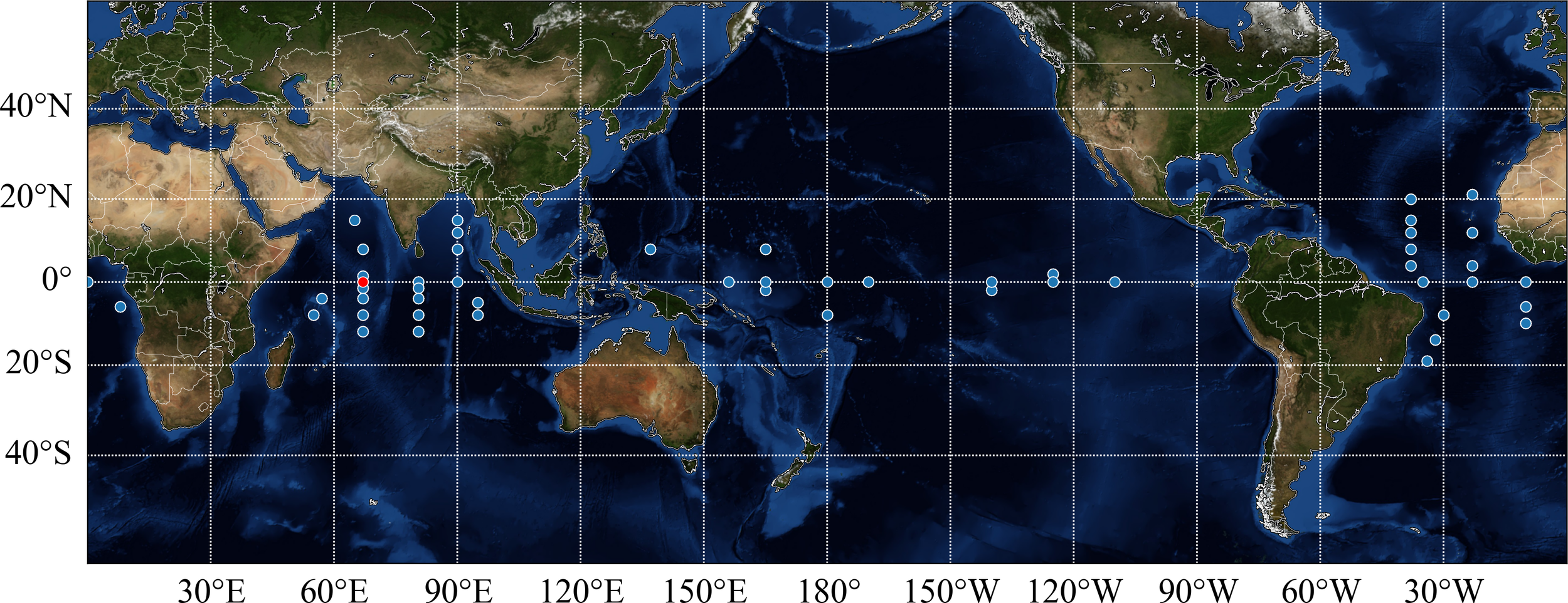
Locations of buoys from the Global Tropical Moored Buoy Array used for comparison indicated as circles.
2.5 Statistical metrics
Two statistical metrics, bias and the root-mean-square error (RMSE), are used to evaluate the performance of the CYGNSS Ocean Surface Heat Flux products, which are calculated for both LHF and SHF.
where X is the CYGNSS latent or sensible heat flux, Y is the buoy latent or sensible heat flux, n is the number of total matchups, is the mean of the CYGNSS latent or sensible heat flux, and is the mean of the buoy latent or sensible heat flux.
2.6 Methodology
To evaluate the performance of the CYGNSS CDR V1.0 and V1.1 heat flux products in the global tropical oceans, collocations between CYGNSS and in situ measurements are processed at each CYGNSS specular point, as shown in the top sub-figures in Figure 2. A spatio-temporal collocating criterion is used to ensure that the acquisition time of the CYGNSS measurement is close to that of in situ measurements from the buoys. To ensure the consistency of heat flux from different sources, the CYGNSS specular points have been produced by in in a temporal window within ±30 min relative to the time of the in situ measurements. Then, the nearest buoy within 25 km is selected according to the distance between the CYGNSS specular point and each buoy location. Finally, the collocations can be obtained from in situ measurements, and the statistical metrics are used to evaluate the performance of the CYGNSS CDR V1.0 and V1.1 heat flux products relative to those estimated by Global Tropical Moored Buoy Array in situ measurements.
Figure 2
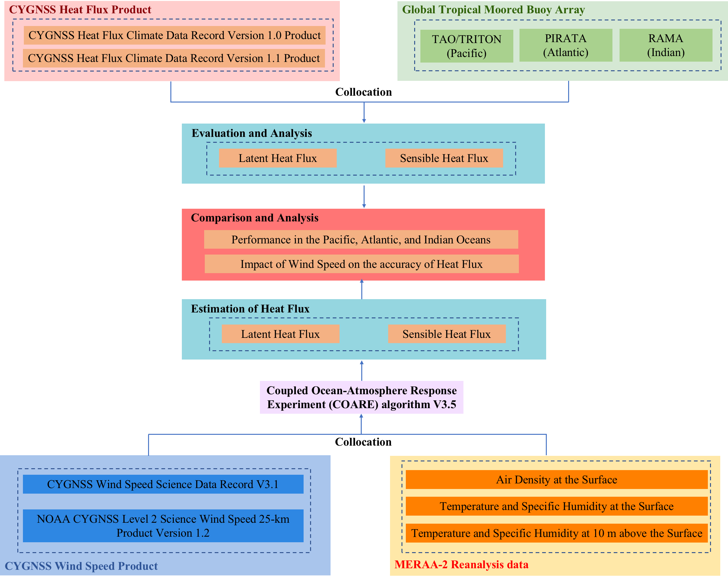
Technical structure and data processing flow of this study of this study.
In addition, as seen in the bottom of Figure 2, matchups between CYGNSS (SDR and NOAA) wind speed products are collocated by the same criteria of spatio-temporal matching, including the density of air at sea level and the specific humidity and temperature at the surface and 10-m above the surface from MERRA-2, respectively. Surface latent and sensible heat fluxes can be calculated by the COARE 3.5 bulk flux algorithm. Thus, the impact of different sea surface wind products from the CYGNSS mission on the accuracy of LHF and SHF is evaluated and analyzed.
3 Results
3.1 Comparison with in situ measurements
In this paper, we use heat flux estimates from the Global Tropical Moored Buoy Array to evaluate the accuracy of the CYGNSS heat flux products in the global tropical oceans. The collocated data from 52 buoys (as shown in Figure 1) are matched with CYGNSS specular points within the above-mentioned spatial and temporal windows. Considering the time range of buoys is different, and the number of buoys used for validating the CYGNSS CDR V1.0 and V1.1 products is also different, Figure 3 shows the spatial distribution of the buoys used for verification: 52 buoys for CYGNSS CDR V1.0 and 45 buoys for CYGNSS CDR V1.1.
Figure 3
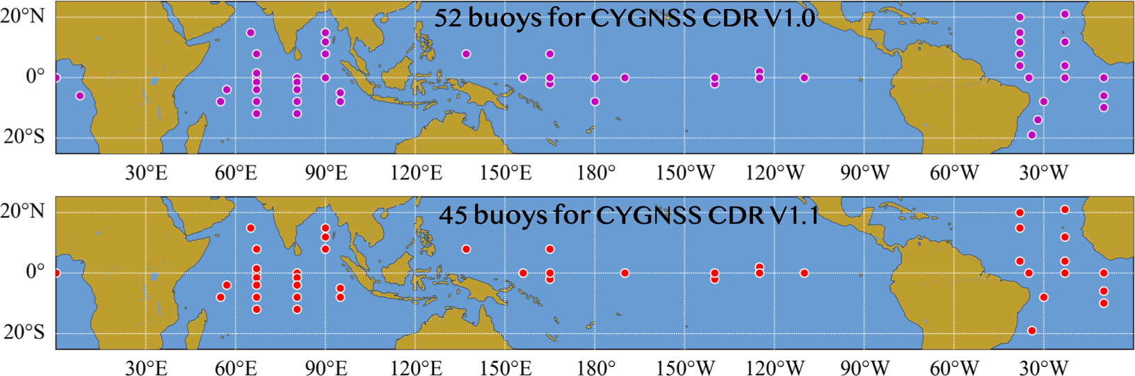
Maps of buoys from the Global Tropical Moored Buoy Array used for comparing the CYGNSS CDR V1.0 and V1.1 heat flux products.
Figure 4 compares LHF/SHF estimates from in situ measurements and from CYGNSS CDR V1.0 and V1.1. The statistical metrics are calculated using Equation 2, which are also shown in Figure 4. From 18 March 2017 to 31 January 2021, LHF/SHF estimates from CYGNSS CDR V1.0 are validated using the in situ heat flux estimates, where the sample size is 147,165, and the RMSEs of CYGNSS LHF/SHF CDR V1.0 are 35.77 W/m2 and 6.75 W/m2 , respectively. For CYGNSS CDR V1.1, the time span is from 1 August 2018 to 28 February 2022, and the RMSEs of CYGNSS LHF/SHF CDR V1.1 are 33.60 W/m2 and 6.67 W/m2 . Note that the sample size is 67,882 after applying CYGNSS flux quality flags (flag!=1), which is less than that of CYGNSS CDR V1.0. This is because some buoys do not provide data for the year of 2022, and the number of buoys for CYGNSS CDR V1.1 is less than that for CYGNSS CDR V1.0.
Figure 4
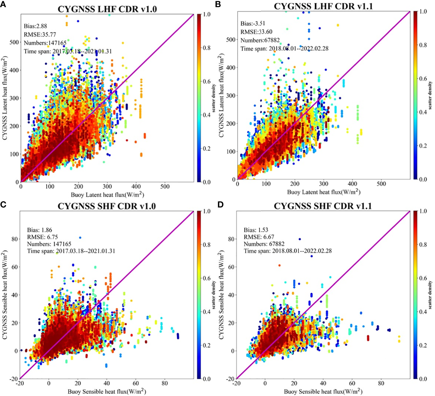
Comparisons between LHF (A, B)/SHF (C, D) estimates from in situ measurements and from CYGNSS CDR V1.0 during 2017-2021 and V1.1 during 2018-2022, respectively. The bias, RMSE, number of matchups, and time span are given in each subfigure. The colorbar is the number density of points, and the purple line shows the 1:1 diagonal.
The highest scatterplot density of LHF occurs between 100 and 200 W/m2 , and that of SHF is between 0 and 15 W/m2. Figure 4A demonstrates that some LHF estimates are overestimated in CYGNSS CDR V1.0 compared with the in situ measurements, whereas overall the CYGNSS CDR V1.1 fluxes agree with the LHF estimates from in situ measurements, as shown in Figure 4B. Figures 4C, D show that there is a discrepancy at high values. In general, both CDR V1.0 and V1.1 fluxes seem to be in agreement with SHF estimates from the in situ measurements, with RMSEs of 6.75 and 6.67 W/m2 , respectively. Overall, it can be seen that the performance of heat flux heat flux estimates from CYGNSS CDR V1.1 is slightly better than that of CYGNSS CDR V1.0.
3.1.2 Accuracy in each tropical ocean basin
CYGNSS can observe the sea surface over the global tropical ocean, providing the chance to estimate the sea surface heat fluxes in each basin. According to Equation 2, we calculate the statistical metrics of latent and sensible heat fluxes for the Pacific, Atlantic, and Indian oceans, respectively. The accuracy assessment in each tropical ocean basin depends on the location of the TAO/TRITON array in the Pacific, PIRATA in the Atlantic, and RAMA in the Indian Ocean, Then, matchups from buoys in each tropical ocean basin are used to estimate the sea surface heat fluxes from CYGNSS CDR V1.0 and V1.1.
Compared to the LHF estimates from the buoys, the CYGNSS mission still shows different latent heat characteristics in the tropical oceans of the Pacific, Atlantic, and Indian oceans as shown in Figure 5. There are some things worth noting. First, LHF is overestimated by CYGNSS CDR V1.0 with a large bias of 10.4 W/m2 , and a positive deviation (bias) is shown for each buoy in the Pacific ocean, especially for the buoy with a latitude of 0°N and a longitude of 180∘ W, where the bias exceeds 30 W/m2. Second, in the Atlantic and Indian oceans, negative deviations appear for some buoys, especially the buoy with a latitude of 10°S and a longitudeof 10°W in the Atlantic ocean, whose bias exceeds –20 W/m2. In addition, we also noticed that the bias of the buoy with a latitude of 19°S and a longitude of 34°W exceeds 40 W/m2. The amount of matchups from this buoy exceeds 2,700, which basically rules out that the bias is not because of insufficient data. There are 21 buoys in the tropical ocean of the Indian ocean, which exhibit a bias of 3.59 W/m2 and an RMSE of 38.14 with respect to the sea surface heat flux. Compared to the accuracy of CYGNSS latent heat in the tropical oceans of the Pacific and the Atlantic oceans, the RMSE of the Indian Ocean is high and the amount of matchups is large, suggesting that the accuracy of CYGNSS heat flux products is low in the tropical regions of the Indian Ocean.
Figure 5
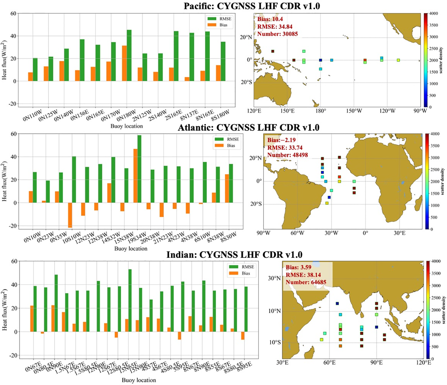
Left column: Biases (yellow bars) and RMSEs (green bars) between CYGNSSLHF CDR V1.0 product and in situ measurements from the tropical oceans of the Pacific, Atlantic, and Indian oceans. Right column: Spatial distribution of buoys from the Global Tropical Moored Buoy Array in each tropical ocean basin. The color density represents the number of matchups for each buoy. The average accuracy (bias and RMSE) and the number of matchups in each tropical ocean are marked in red font.
For CYGNSS LHF CDR V1.1, Table 3 shows the statistical metrics of matchups in the tropical oceans of the Pacific, Atlantic, and Indian oceans. More details are shown in Figure A1 in Appendix. In the Pacific Ocean, the accuracy of CDR V1.1 is slightly better than that of CDR V1.0, with a bias of 7.58 W/m2 and an RMSE of 32.60 W/m2 . In addition, we also noticed that the number of matchups is 13,028, which is less than that of CYGNSS LHF CDR V1.0. From Figure A1 in Appendix, the RMSE of the buoy (marked in rectangle with red border) with a latitude of 8°N and a longitude of 165°E exceeds 40 W/m2. This difference between CYGNSS and the the buoy is inconsistent due to insufficient data (less than 300). It can be seen from Table 3 that the biases are negative in the Atlantic and Indian oceans, which are similar to those of CYGNSS CDR V1.0; especially, the deviation at a latitude of 10°S and a longitude of 10°W in the Atlantic Ocean exceeds –20 W/m2 (Figure A1 in Appendix). However, the accuracy (RMSE) of CDR V1.1 is slightly better than that of CDR V1.0 in the Atlantic and Indian Oceans.
Table 3
| Version | Tropical ocean | Latent heat flux | Sensible heat flux | ||
|---|---|---|---|---|---|
| Bias (m/s) | RMSE (m/s) | Bias (m/s) | RMSE (m/s) | ||
| CYGNSS V1.0 | Pacific Ocean | 10.4 | 34.84 | 1.73 | 6.88 |
| Atlantic Ocean | -2.19 | 33.74 | 1.75 | 5.71 | |
| Indian Ocean | 3.59 | 38.14 | 2.09 | 7.47 | |
| CYGNSS V1.1 | Pacific Ocean | 7.58 | 32.60 | 1.27 | 6.82 |
| Atlantic Ocean | -10.27 | 31.76 | 1.34 | 5.61 | |
| Indian Ocean | -2.95 | 35.73 | 1.87 | 7.44 | |
Statistical metrics (bias and RMSE) calculated from the matchups between CYGNSS and in situ measurements in the Pacific, Atlantic, and Indian oceans.
In terms of sensible heat, Table 3 and Figure A2 (in Appendix) give the statistical metrics and and a histogram of CYGNSS SHF CDR V1.0 and V1.1 for bias (yellow bars) and RMSE (green bars), which demonstrate a good agreement between CYGNSS and in situ measurements from buoys. For the deviation in the tropical oceans of the Pacific, Atlantic, and Indian oceans, it can be seen that CYGNSS SHF CDR V1.0 and V1.1 overestimate the sensible heat relative to buoys, especially in the Indian Ocean (a large bias of 2.09 W/m2). In the Pacific, we also noticed that the deviation of CYGNSS SHF CDR V1.1 exceeds in –3 W/m2 and RMSE exceeds 20 W/m2 at a latitude of 8°N and a longitude of 165°E (Figure A2 in Appendix). However, the deviation of CYGNSS SHF CDR V1.0 is close to 0 W/m2 at this buoy (Figure A2 in Appendix). Except for this unusual buoy, the two versions of CYGNSS can give similar accuracies for SHF on the whole, which is consistent with in situ measurements from the buoy.
3.2 Annual variation characteristics of LHF/SHF in CYGNSS CDR products
To analyze the heat flux characteristics of LHF/SHF estimated by CYGNSS during this mission, the annual variation trends are investigated and analyzed according to several typical buoys. Figure 6 shows the ability of the CYGNSS mission to estimate heat flux at a specific location, which is consistent with those estimated from buoys. It can be seen that the buoys had missing data in the Pacific and Atlantic at various times: 2018.03∼2018.08 for buoy (8°N, 137°E) in the Pacific (Figure 6A), and 2018.11∼2019.01, 2020.08∼2022.01 and 2021.07∼2021.11 for buoy (20°N,38°W) in the Atlantic (Figure 6D). For buoy (8°S, 95°E) in the Indian Ocean, the heat flux data are normal and continuous. The blue dotted-line represents the CYGNSS LHF CDR V1.0 product, and the orange dotted-line represents the heat flux estimated by buoy data, as shown in Figure 6E. From the three heat flux products, it can see that there is a peak in August of each year, especially in 2017, 2018, and 2019. There is an obvious growth trend between July and August, as well as an obvious downward trend between September and November. However, these phenomena do not occur in the other two buoys in the Pacific and the Atlantic oceans. Thus, the CYGNSS mission produce heat flux estimates over the tropical ocean, providing an important reference for analyzing global tropical ocean heat flux changes.
Figure 6
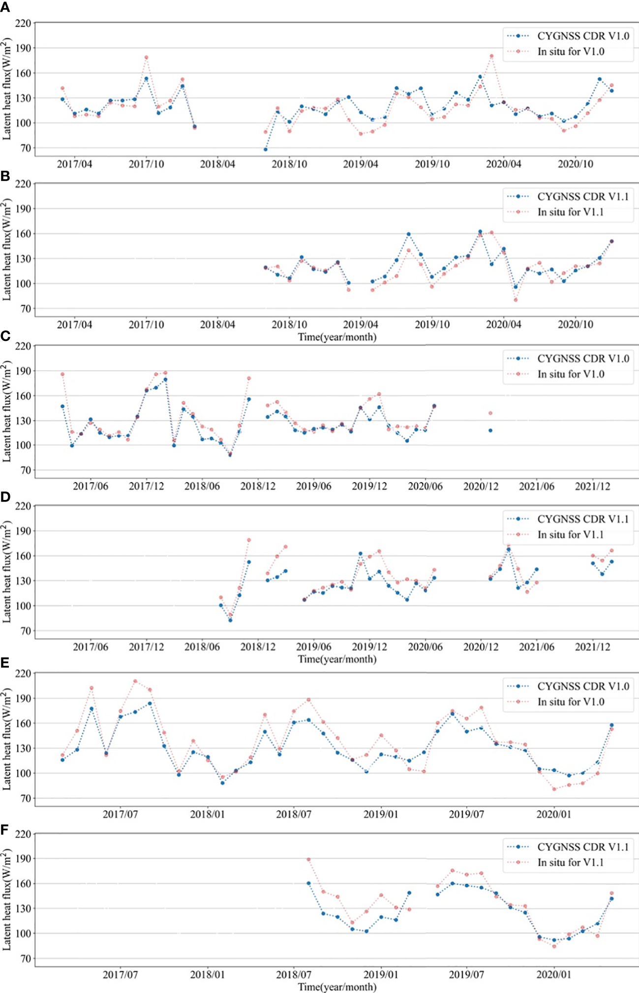
Comparisons of CYGNSS LHF CDR products and in situ in situ buoys heat flux in the tropical oceans of the Pacific (A, B:8°N, 137°E), Atlantic C, D:20°N, 38°W), and Indian (E, F:8 °S, 95°E) oceans, respectively.
3.3 Impact of wind speed on the accuracy of LHF/SHF
3.3.1. LHF/SHF estimated by CYGNSS SDR and NOAA wind speed
In this study, the latest versions of wind speed products are used to analyze the impact of wind speed on the accuracy of LHF/SHF, including the NOAA CYGNSS Level 2 V1.2 and SDR V3.1 wind speed products. Table 4 gives a summary of CYGNSS Level 2 wind speed product information, including product version and time span.
Table 4
| Wind speed products | Time span |
|---|---|
| NOAA CYGNSS Level 2 V1.2 | 2017.05.01–2022.02.28 |
| CYGNSS Level 2 SDR V3.1 | 2018.08.01–2022.02.28 |
CYGNSS Level 2 wind speed products and time spans for estimating heat flux.
According to Equation 1, both wind speed products from the CYGNSS satellite constellation are used to derive the surface heat fluxes (LHF/SHF) using the sea and air thermodynamic variables of temperature and humidity. To ensure the consistency of the sea and air thermodynamic variables of the CYGNSS CDR heat flux products, according to the time and position at each specular point, the Level 2 wind speed is first spatio-temporally collocated with LHF/SHF estimated by the buoys, and then collocated with the Level 2 heat flux product to obtain the thermodynamic parameters provided by NASA MERRA-2 for calculating the heat flux.
3.3.2. Comparisons of CYGNSS heat fluxes
For LHF, CYGNSS NOAA V1.2 can provide stable wind speeds to estimate heat flux with a bias of 5.83 W/m2 and an RMSE of 29.68 W/m2 . An improvement (RMSE) of 17% for the CYGNSS LHF product is obtained using the CYGNSS NOAA V1.2 wind speed product. However, the number of data pairs matched with the buoy decreased significantly from 147,165 to 54,219. During NOAA V1.2 wind speed inversion, a large number of outliers were identified and eliminated through quality control. From Figure 7A, it can be seen that the LHF estimated from CYGNSS NOAA V1.2 winds is consistent with that estimated from buoy data compared to the CYGNSS CDR V1.0 heat flux product (Figure 4A). In terms of deviation (CYGNSS – Buoy), LHF is overestimated by CYGNSS NOAA V1.2. It can be seen from Figure 7C that the bias and RMSE of the LHF estimated from CYGNSS SDR V3.1 are –1.39 W/m2 and 33.03 W/m2, respectively, which are slight better than those of the CYGNSS LHF CDR V1.1 product during the same period of 2018.08.01–2022.02.28.
Figure 7
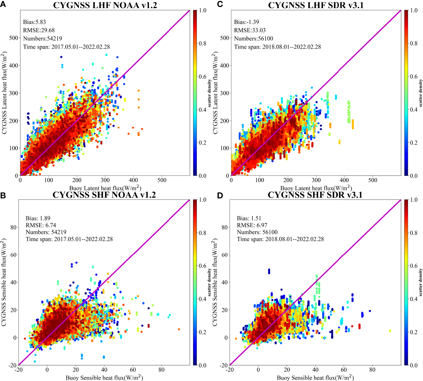
Comparisons between LHF (A, B)/SHF (C, D) estimates from in situ measurements and from CYGNSS NOAA V1.2 during 2017-2021 and SDR V3.1 during 2018-2022, respectively. The bias, RMSE, number of matchups, and time span are given in each subfigure. The colorbar is the number density of points, and the purple line shows the 1:1 diagonal.
Figures 7B, D also illustrate the performance of the CYGNSS NOAA V1.2 and CYGNSS SDR V3.1 wind products in estimating SHF. It is noted that CYGNSS SDR V3.1 gives a large RMSE of 6.97 W/m2 , whereas the RMSE of the other SHF product is ∼ 6.7 W/m2 . By using different wind speed products to estimate SHF, it is found that the impact on the accuracy of SHF is minor, and there is no obvious improvement in accuracy.
3.3.3. Performance in the Pacific, Atlantic, and Indian Oceans
According to the RAMA, PIRATA, and TRITON, the performance of CYGNSS LHF/SHF NOAA V1.2 is analyzed, as shown in Figure 8. The characteristics of the NOAA V1.2 LHF/SHF product are the same as that of CYGNSS CDR V1.0, which has a positive deviation for every buoy in the Pacific Ocean, and RMSE decreases from 34.84 W/m2 to 29.59 W/m2 (15% improvement). In addition, improvements of the Indian Ocean and the Atlantic, it has improved to varying degrees, 11.6% and 26.8%, respectively. It is noted that the buoy with a latitude of 19°S and a longitude of 34°W also gives a large deviation (> 50 W/m2 ) and RMSE (> 60 W/m2). For the LHF product, there is no improvement in accuracy in any tropical ocean basin.
Figure 8
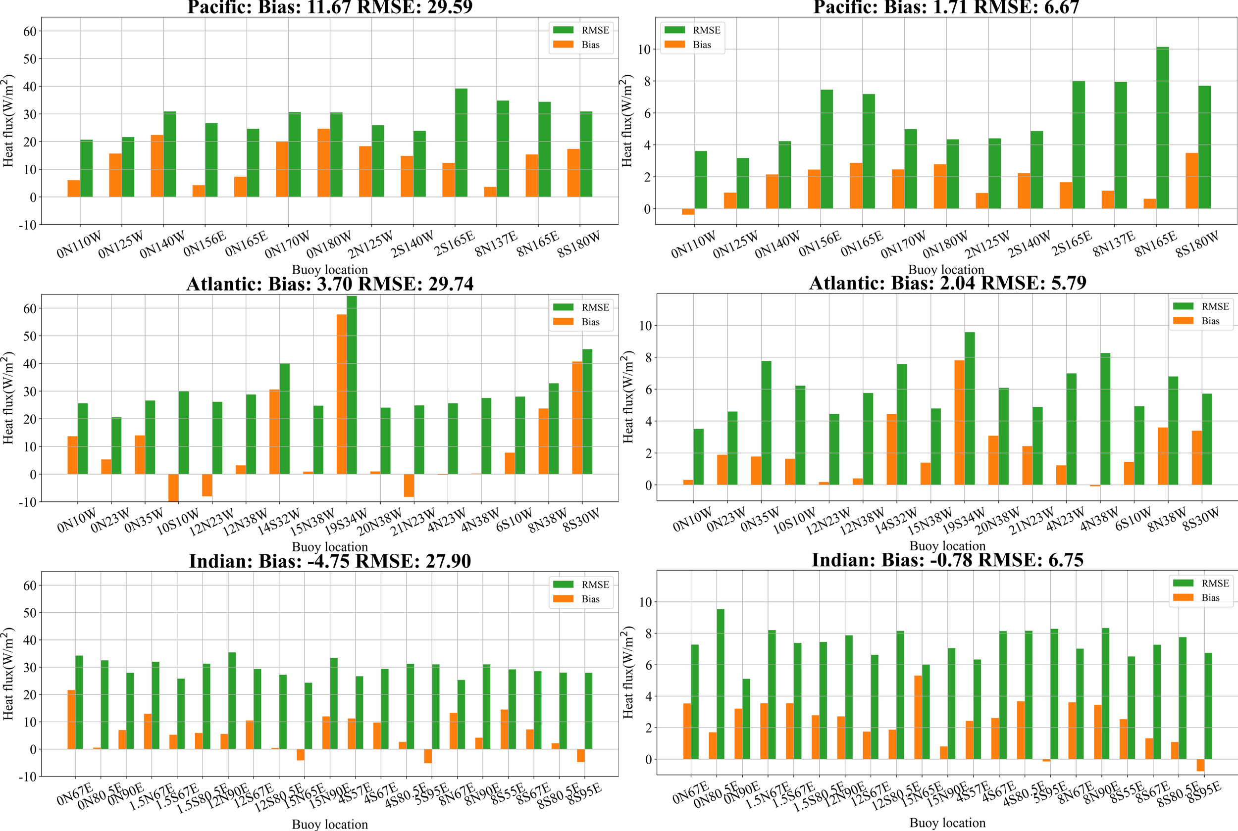
Left column: Performance of the CYGNSS LHF NOAA V1.2 product compared to the TAO/TRITON array in the Pacific, PIRATA in the Atlantic, and RAMA in the Indian Ocean. Right column: The same for the CYGNSS SHF NOAA V1.2 product.
4 Conclusions
A preliminary evaluation of the heat flux (LHF/SHF) estimates from the remotely sensed wind speed measurements of the CYGNSS mission during the period of 2017–2022 is performed. We systematically compare temporally and spatially coincident CYGNSS heat fluxes and those estimated from various tropical moored buoy systems (i.e., TAO, TRITON, PIRATA, and RAMA). The comparisons show that the CYGNSS CDR V1.1 heat flux is in good agreement with estimates from the buoys, with overall average RMSEs of 33.60 W/m2 and 6.77 W/m2 for LHF/SHF, respectively. The overall average bias is –3.51 W/m2 , demonstrating that CYGNSS LHF CDR V1.1 underestimates compared to the in situ measurements for global tropical oceans, whereas SHF CDR V1.1 slightly overestimates, with a bias of 1.53 W/m2 . Furthermore, the differences in each tropical ocean basin are investigated according to the heat flux estimates from the TAO/TRITON, PIRATA, and RAMA buoys. It is found the CYGNSS heat flux in the Atlantic Ocean has better performance than that in the Pacific and Indian oceans. For CYGNSS CDR V1.0 and V1.1, it is shown that the SHF product is slightly overestimated, with a a positive bias in the Pacific, Atlantic, and Indian oceans. Additionally, it should be noted that the amount of matchups between CYGNSS and the the buoys is limited, which may have resulted in some uncertainty in the evaluation accuracy of CYGNSS heat flux products in each tropical ocean basin. In addition, the impact on the accuracy of LHF/SHF estimates is investigated by the CYGNSS NOAA V1.2 and CYGNSS SDR V3.1 wind products. The results illustrate that CYGNSS NOAA V1.2 winds can significantly improve the accuracy of LHF estimates by 17%, and both wind products have almost no impact on SHF estimates. Overall, the heat flux products acquired from the CYGNSS mission in 2017–2022 are valuable for practical use.
Funding
This work was supported by the Scientific Research Fund of the Second Institute of Oceanography, MNR, grand no. JB2205, as well as the Innovation Group Project of Southern Marine Science and Engineering Guangdong Laboratory (Zhuhai) (No. 311021004), by the European Space Agency and Ministry of Science and Technology Dragon 5 Cooperation Programme under Grant 58009. We also thank the staff of the satellite ground station, satellite data processing and sharing center, and marine satellite data online analysis platform of the State Key Laboratory of Satellite Ocean Environment Dynamics, Second Institute of Oceanography, Ministry of Natural Resources (SOED/SIO/MNR), for their help with data collection and processing.
Publisher’s note
All claims expressed in this article are solely those of the authors and do not necessarily represent those of their affiliated organizations, or those of the publisher, the editors and the reviewers. Any product that may be evaluated in this article, or claim that may be made by its manufacturer, is not guaranteed or endorsed by the publisher.
Statements
Data availability statement
The original contributions presented in the study are included in the article/supplementary material. Further inquiries can be directed to the corresponding authors.
Author contributions
XL and JY designed the study and managed the project. XL and WL led the research, interpreted the data, drew figures, and wrote the manuscript. YY collected in situ buoy observation data calculated surface heat fluxes, and analyzed the satellite-based surface heat flux datasets from the CYGNSS mission. XL and WL compared satellite estimates with buoy observations. YY and WL contributed some useful scripts for this study. JY and YY were involved with reviewing and editing the manuscript. All authors contributed to improving the manuscript. All authors contributed to the article and approved the submitted version.
Conflict of interest
The authors declare that the research was conducted in the absence of any commercial or financial relationships that could be construed as a potential conflict of interest.
References
1
Back L. E. Bretherton C. S. (2005). The relationship between wind speed and precipitation in the Pacific ITCZ. J. Climate18, 4317–4328. doi: 10.1175/JCLI3519.1
2
Bentamy A. Katsaros K. B. Mestas-NunEz A. M. Drennan W. M. Forde E. B. Roquet H. (2003). Satellite estimates of wind speed and latent heat flux over the global oceans. J. Climate16, 637–656. doi: 10.1175/1520-0442(2003)016<0637:SEOWSA>2.0.CO;2
3
Bentamy A. Piollé J. Grouazel A. Danielson R. Gulev S. Paul F. et al . (2017). Review and assessment of latent and sensible heat flux accuracy over the global oceans. Remote Sens. Environ.201, 196–218. doi: 10.1016/j.rse.2017.08.016
4
Bharti V. Schulz E. Fairall C. W. Blomquist B. W. Manton M. J. (2019). Assessing surface heat flux products with in situ observations over the Australian sector of the southern ocean. J. Atmos. Ocean Tech.36, 1849–1861. doi: 10.1175/JTECH-D-19-0009.1
5
Businger J. A. (1982). The fluxes of specific enthalpy, sensible heat and latent heat near the earth’s surface. J. Atmos.39, 1889–1894. doi: 10.1175/1520-0469(1982)039<1889:TFOSES>2.0.CO;2
6
Chou S. H. Nelkin E. Ardizzone J. Atlas R. M. Shie C. L. (2002). Surface turbulent heat and momentum fluxes over global oceans based on the goddard satellite retrievals, version 2 (GSSTF2). J. Climate16, 3256–3273. doi: 10.1175/1520-0442(2003)016<3256:STHAMF>2.0.CO;2
7
Clarizia M. P. Ruf C. S. Jales P. Gommenginger C. (2014). Spaceborne GNSS-R minimum variance wind speed estimator. IEEE Trans. Geosci. Remote Sens.52, 6829–6843. doi: 10.1109/TGRS.2014.2303831
8
Crespo J. A. Posselt D. J. (2019). Development and early results of the surface heat flux product for the CYGNSS mission (Jet Propulsion Laboratory, California Institute of Technology). Tallahassee techreport.
9
Crespo J. A. Posselt D. J. Asharaf S. (2019). CYGNSS surface heat flux product development. Remote Sens.11, 2294. doi: 10.3390/rs11192294
10
Cronin M. F. Gentemann C. L. Edson J. Ueki I. Zhang D. (2019). Air-sea fluxes with a focus on heat and momentum. Front. Mar. Sci.6, 430. doi: 10.3389/fmars.2019.00430
11
CYGNSS (2020) CYGNSS level 2 ocean surface heat flux climate data record version 1.0. ver. 1.0 (Accessed 2022-04-10).
12
Edson J. Jampana V. Weller R. Bigorre S. Plueddemann A. Fairall C. et al . (2013). On the exchange of momentum over the open ocean. J. Phys. Oceanogr.43, 1589–1610. doi: 10.1175/JPO-D-12-0173.1
13
Fairall C. Bradley E. Rogers D. Edson J. Young G. (1996). Bulk parameterization of air-sea fluxes for tropical ocean-global atmosphere coupled ocean-atmosphere response experiment. J. Geophys. Res.101, 3747–3764. doi: 10.1029/95JC03205
14
Gao S. Chiu L. S. Shie C. L. (2013). Trends and variations of ocean surface latent heat flux: Results from GSSTF2c data set. Geophys. Res. Lett.40, 380–385. doi: 10.1029/2012GL054620
15
Gleason S. T. Hodgart S. Sun Y. Gommenginger C. Unwin M. (2005). Detection and processing of bistatically reflected GPS signals from low earth orbit for the purpose of ocean remote sensing. IEEE Trans. Geosci. Remote Sens.43, 1229–1241. doi: 10.1109/TGRS.2005.845643
16
Grodsky S. A. Bentamy A. Carton J. A. Pinker R. T. (2009). Intraseasonal latent heat flux based on satellite observations. J. Climate22, 4539–4556. doi: 10.1175/2009JCLI2901.1
17
Hartmann D. L. (1994). “Chapter 4 the energy balance of the surface,” in Global physical climatology, vol. 56. (Amsterdam, Academic Press), 81–114. doi: 10.1016/S0074-6142(08)60561-6
18
Jing C. Niu X. Duan C. Lu F. Yang X. (2019). Sea Surface wind speed retrieval from the first Chinese GNSS-R mission: Technique and preliminary results. Remote Sens.11, 3013. doi: 10.3390/rs11243013
19
KonDa M. Imasato N. Shibata A. (1996). Analysis of the global relationship of biennial variation of sea surface temperature and air-sea heat flux using satellite data. J. Oceanogr.52, 717–746. doi: 10.1007/BF02239462
20
Large W. G. Pond S. (1982). Sensible and latent heat flux measurements over the ocean. J.phy.oceanogr.12, 464–482. doi: 10.1175/1520-0485(1982)012<0464:SALHFM>2.0.CO;2
21
Li W. Cardellach E. Ribó S. Oliveras S. Rius A. (2022). Exploration of multi-mission spaceborne GNSS-R raw if data sets: Processing, data products and potential applications. Remote Sens.14, 1344. doi: 10.3390/rs14061344
22
Liu W. Katsaros K. Businger J. (1979). Bulk parameterization of the air-sea exchange of heat and water vapor including the molecular constraints at the interface. J. Atmos. Sci.36, 2052–2062. doi: 10.1175/1520-0469(1979)036<1722:BPOASE>2.0.CO;2
23
Kubota M. Iwasaka N. Kizu S. Konda M. Kutsuwada K. . (2002). Japanese Ocean flux data sets with use of remote sensing observations (J-OFURO). J. Oceanogr.58, 213–215. doi: 10.1023/A:1015845321836
24
Pinker R. T. Bentamy A. Katsaros K. B. Ma Y. Li C. (2014). Estimates of net heat fluxes over the Atlantic ocean. J. Geophys. Res. Oceans119, 410–427. doi: 10.1002/2013JC009386
25
Ruf C. Atlas R. Chang P. Clarizia M. P. Zavorotny V. (2016). New ocean winds satellite mission to probe hurricanes and tropical convection. Bull. Am. Meteorol. Soc97, 385–395. doi: 10.1175/BAMS-D-14-00218.1
26
Ruf C. Balasubramaniam R. (2018). Development of the CYGNSS geophysical model function for wind speed. IEEE J. Sel. Topics Appl. Earth Obs. Remote Sens.12, 66–77. doi: 10.1109/JSTARS.2018.2833075
27
Said F. Jelenak Z. Park J. Soisuvarn S. Chang P. S. (2019). A ’track-wise’ wind retrieval algorithm for the CYGNSS mission. IEEE Int. Geosci. Remote Sens. Symp., 8711–8714. doi: 10.1109/IGARSS.2019.8898099
28
Shie C. Hilburn K. A. (2011). The Goddard satellite-based surface turbulent fluxes (GSSTF) datasets and the Uncertainties/Impact due to the SSM/I brightness temperature. In AGU Fall Meeting Abstractsvol. 2011, IN21A–I1417.
29
Tauro F. Maltese A. Giannini R. Harfouche A. (2022). Latent heat flux variability and response to drought stress of black poplar: A multi-platform multi-sensor remote and proximal sensing approach to relieve the data scarcity bottleneck. Remote Sens. Environ.268, 112771. doi: 10.1016/j.rse.2021.112771
30
Tomita H. Kutsuwada K. Kubota M. Hihara T. (2021). Advances in the estimation of global surface net heat flux based on satellite observation: J-OFURO3 v1.1. Front. Mar. Sci.8, 612361. doi: 10.3389/fmars.2021.612361
31
Unwin M. Jales P. Tye J. Gommenginger C. Foti G. Rosello J. (2017). Spaceborne GNSS-reflectometry on TechDemoSat-1: Early mission operations and exploitation. IEEE J. Sel. Top. Appl. Earth Obs. Remote Sens.9, 4525–4539. doi: 10.1109/JSTARS.2016.2603846
32
Wang D. Zeng L. Li X. Shi P. (2013). Validation of satellite-derived daily latent heat flux over the South China Sea, compared with observations and five products. J. Atmos. Ocean. Tech.30, 1820–1832. doi: 10.1175/JTECH-D-12-00153.1
33
Webster P. Lukas R. (1992). Toga coare: The coupled ocean-atmosphere response experiment. Bull. Amer. Meteor. Soc73, 1376–1416. doi: 10.1175/1520-0477(1992)073<1377:TCTCOR>2.0.CO;2
34
Yang G. Bai W. Wang J. Hu X. Zhang P. Sun Y. et al . (2022). FY-3E GNOS II GNSS reflectometry: Mission review and first results. Remote Sens.14, 988. doi: 10.3390/rs14040988
35
Yu L. Weller R. A. Sun B. (2004). Improving latent and sensible heat flux estimates for the Atlantic ocean, (1988 99) by a synthesis approach. J.Climate17, 373–393. doi: 10.1175/1520-0442(2004)017<0373:ILASHF>2.0.CO;2
36
Zeng L. Shi P. Liu W. T. Wang D. (2009). Evaluation of a satellite-derived latent heat flux product in the South China Sea: A comparison with moored buoy data and various products. Atmos. Res.94, 91–105. doi: 10.1016/j.atmosres.2008.12.007
37
Zhou L. T. Chen G. Wu R. (2015). Change in surface latent heat flux and its association with tropical cyclone genesis in the Western North Pacific. Theor. Appl. Climatol.119, 221–227. doi: 10.1007/s00704-014-1096-0
Appendix
Figure A1
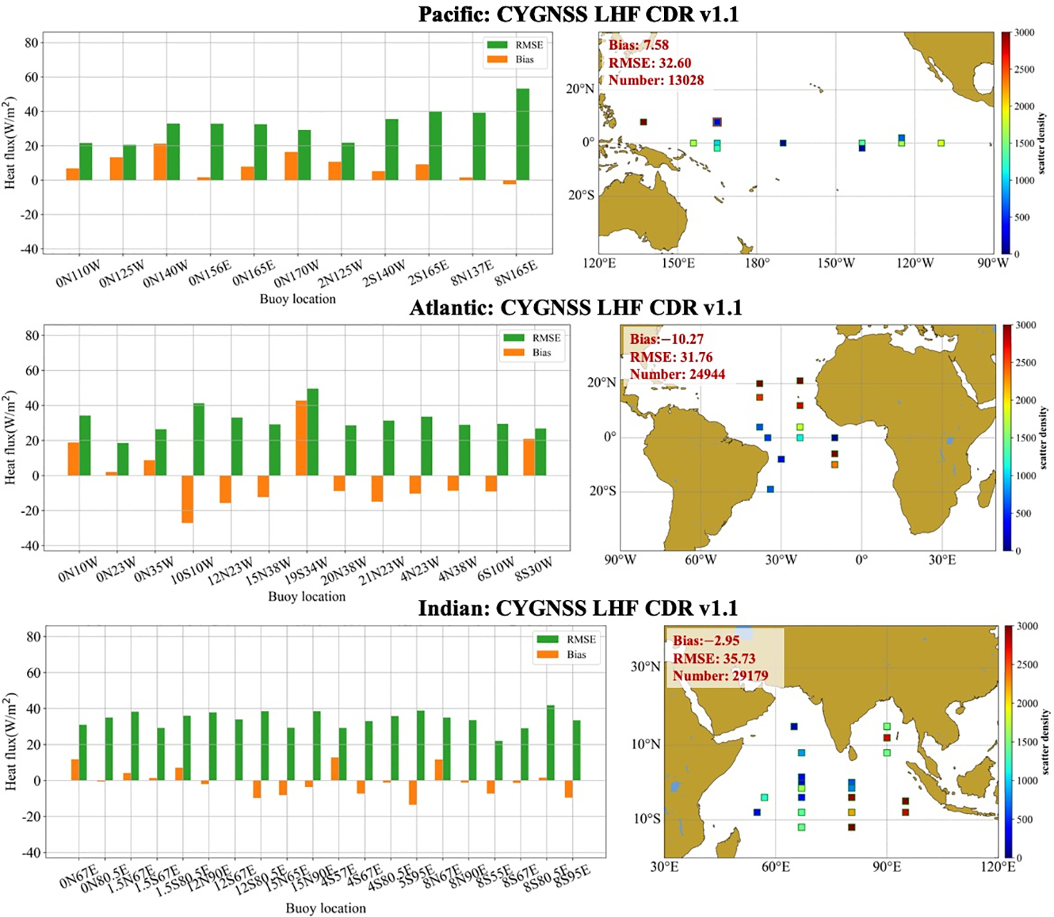
Left column: Biases (yellow bars) and RMSEs (green bars) between the CYGNSS LHF CDR V1.1 product and in situ measurements from the tropical oceans of the Pacific, Atlantic, and Indian oceans. Right column: Spatial distribution of buoys from the Global Tropical Moored Buoy Array in each tropical ocean basin. Color density represents the number of matchups for each buoy. The average accuracy (bias and RMSE) and the number of matchups in each tropical ocean are marked in red font.
Figure A2
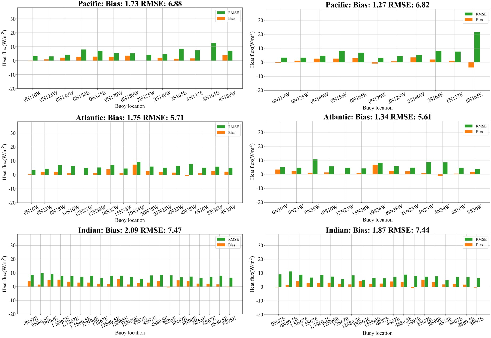
Left column: Biases (yellow bars) and RMSEs (green bars) between the CYGNSS SHF CDR V1.0 product and in situ measurements from the tropical oceans of the Pacific, Atlantic, and Indian oceans. Right column: The same for the CYGNSS SHF CDR V1.1 product. The same for the CYGNSS SHF CDR V1.1 product.
Summary
Keywords
global navigation satellite system reflectometry (GNSS-R), cyclone GNSS (CYGNSS), surface heat fluxes, latent heat flux, sensible heat flux, tropical ocean
Citation
Li X, Yang J, Yan Y and Li W (2022) Exploring CYGNSS mission for surface heat flux estimates and analysis over tropical oceans. Front. Mar. Sci. 9:1001491. doi: 10.3389/fmars.2022.1001491
Received
23 July 2022
Accepted
24 October 2022
Published
18 November 2022
Volume
9 - 2022
Edited by
Lei Ren, Sun Yat-sen University, China
Reviewed by
Patrizia Savi, Politecnico di Torino, Italy; Haokui Xu, University of Michigan, United States
Updates
Copyright
© 2022 Li, Yang, Yan and Li.
This is an open-access article distributed under the terms of the Creative Commons Attribution License (CC BY). The use, distribution or reproduction in other forums is permitted, provided the original author(s) and the copyright owner(s) are credited and that the original publication in this journal is cited, in accordance with accepted academic practice. No use, distribution or reproduction is permitted which does not comply with these terms.
*Correspondence: Jingsong Yang, jsyang@sio.org.cn; Weiqiang Li, weiqiang@ice.csic.es
This article was submitted to Ocean Observation, a section of the journal Frontiers in Marine Science
Disclaimer
All claims expressed in this article are solely those of the authors and do not necessarily represent those of their affiliated organizations, or those of the publisher, the editors and the reviewers. Any product that may be evaluated in this article or claim that may be made by its manufacturer is not guaranteed or endorsed by the publisher.