Abstract
As one of the most sensitive factors in the sea–land interaction zone, the shoreline is significantly influenced by natural processes and anthropogenic activities. Monitoring long-term shoreline changes offers a basis for the integrated management and protection of coastal zones. The spatiotemporal distribution and the utilization types of shorelines had changed a lot, along with the advancement of the socioeconomics of the countries around the South China Sea (SCS) since 1980. However, the changes in shoreline characteristics for a long time around the whole SCS under anthropogenic influence remain uncertain. Using Landsat and high-resolution satellite images, this study monitored the changes in the spatial location and type of shorelines around the SCS from 1980 to 2020. Additionally, the possible reasons for the shoreline changes around the SCS were analyzed. The results showed the following: 1) the length of shorelines around the SCS maintained growth, especially in the 1990s, which increased by 734.8 km, from 28,243.8 km (1990) to 28,978.6 km (2000). 2) The proportion of natural shorelines around the SCS decreased from 92.4% to 73.3% during the past 40 years. Bedrock and mangrove shorelines disappeared most sharply by 34.2% and 21.6%, respectively. The increase of artificial shorelines was mostly driven by the expansion of constructed and aquaculture dikes. 3) The spatial location changes of most artificial shorelines can be attributed to seaward advancement, with an average advancing speed of 7.98 m/year. Of the natural shorelines, 58.4% changed in terms of their location (30.4% advancement and 28.0% retreat). Most natural shorelines around the SCS were threatened by erosion, but the extent of which was largely determined by the shorelines’ own stability, with less influence from the surrounding environment. Artificialization was the most prominent feature of shorelines around the SCS over the past 40 years, which was closely related to the original types of shorelines and the socioeconomic conditions of the area where they are located, and often accompanied by dramatic changes in shoreline morphology and spatial location. In addition, human interventions were not only the dominant factor in shoreline artificialization but also a major driver of natural shoreline protection.
Introduction
The coastal zone is the most densely populated and contains key infrastructure and a valuable ecosystem, which is affected by both natural processes and anthropogenic activities (Martinez et al., 2007; Temmerman et al., 2013; Mentaschi et al., 2018). The shoreline is naturally dynamic and one of the most sensitive factors in the sea–land interaction zone, shifting over time in response to coastal geomorphological processes and anthropogenic activities (Nguyen et al., 2015). The shoreline is not only seen as the embodiment of coastal ecosystem evolution but also as a significant symbol of coastal zone exploitation activities (Zhang and Hou, 2020; Duan et al., 2021). Shorelines can be considered special natural resources that can be exploited, protected, and provide ecological and economic value (Currin, 2019). With the impact of global climate change such as sea level rise, global warming, weather extremes, and anthropogenic activities including reclamation and nearshore engineering, the utilization type and the spatial location of the shorelines have changed a lot. Thus, monitoring and understanding changes in shorelines are of great importance to their protection and reasonable use, as stated in Sustainable Development Goals (SDGs) 14: “conserve and sustainably use the oceans, seas, and marine resources for sustainable development” (Wright et al., 2017).
Shorelines can be defined as the physical interface of land and water in the idealized situation (Dolan et al., 1980). Due to nearshore hydrodynamic processes (e.g., ocean waves, tides, and currents, among others), it is difficult to obtain the precise location of shorelines on a large scale. Therefore, the shoreline indicator is widely used as a proxy to represent the “true” shoreline location (Boak and Turner, 2005; McAllister et al., 2022). There are many physical features that can be used as shoreline indicators, which include vegetable line, debris line, wet/dry boundaries, high water line (HWL), mean high water line (MHWL), instantaneous high water line (IHWL), and low water line (LWL) (Zhang and Hou, 2020). The MHWL, which can be obtained by correcting the IHWL to eliminate the effect of tides, is widely considered to be a useful shoreline indicator for easy identification in remote sensing images (Zhang and Hou, 2020).
Research on the changes in shorelines was limited by technical constraints; usually focuses on the changes of shorelines along small areas such as bays, estuaries, or cities with similar natural and socioeconomic conditions; and lacks data on the variability of multiple shoreline types over larger spatial and temporal scales (Schwimmer, 2001; Turner et al., 2021). Kuleli et al. found that the coastal Ramsar wetlands of Turkey had been under threat of erosion for many years (1989–2009) using Landsat images and the Digital Shoreline Analysis System (DSAS). Agriculture, damming rivers, sand extraction from beaches, and other anthropogenic activities had caused most of this threat (Kuleli et al., 2011). Based on multi-temporal topographic maps, remote sensing images, and field surveys covering the entire coastal zone of Mainland China, Hou et al. have extracted shoreline data at six stages for 70 years. They found that the scale and speed of shoreline artificialization were dramatic: more than 68% of shorelines expanded toward the sea, with an average rate of 24.3 m/year, while over 22% of shorelines retreated toward the land, with an average rate of −3.27 m/year; only 10% of shorelines remained stable. The physical factors tended to gradually give way to human factors, such as sea reclamation and engineering protection, which have significantly altered the intrinsic evolution processes of the shorelines of China (Hou et al., 2016). Manuela et al. investigated the spatiotemporal shift of shorelines along the Gulf of Cagliari across a time frame of 62 years (1954–2016) and found that these shorelines had undergone great modification as a result of the intense anthropogenic activities impacting the coastal areas (Biondo et al., 2020).
Except for Japan, Netherlands, Singapore, and China, there are a few large-scale reclamation activities in other countries around the world, but the increasing exploitation of the coastal zone, including agriculture and aquaculture development, the manufacturing and maritime industry, and tourism and recreation, as well as natural factors such as extreme weathers, global warming, sea level rise, and the reduction of river sediments, have created more and more problems and threats on the coastal zone (Wu and Hou, 2016). Research studies on shorelines have focused more on the spatial location change of natural shorelines, such as sandy and mangrove shorelines, and relatively little research has been done on the changes in shoreline utilization types and spatial location caused by anthropogenic activities. An understanding of the characteristics of shoreline changes under intense anthropogenic activities and various natural and socioeconomic environments is still lacking, especially on large spatial and temporal scales. Compared with other regions of the world, the socioeconomic development pattern and the diverse natural environments of the countries around the South China Sea (SCS) provide an ideal case to examine the influence of anthropogenic activities on shoreline changes. To fill these gaps, our study intended to establish a shoreline dataset around the SCS for the past 40 years, when the economy of the surrounding countries experienced great development, and explore the characteristic driving factors of these shoreline changes.
Data and methods
Study area
Located at the heart of the Indo-Pacific region, the SCS bridges the Indian and Pacific Oceans and is also a crucial international shipping lane. The SCS is a semi-closed marginal sea located in the tropics, spanning the Northern and the Southern Hemisphere, and is surrounded by the South China Continent, Indochinese Peninsula, and Malay Archipelago. The areas surrounding the SCS are dominated by a tropical climate, with a large amount of precipitation, which created dense rivers with vast deltas and alluvial plains (Sidi et al., 2003; Wit et al., 2015; Beck et al., 2018) (Figure 1). To its north and west, the SCS is bordered by South China and the Indochina Peninsula; to the east and south, it is surrounded by a chain of islands, from Luzon in the north to Borneo in the south. The continent side to the north and west is mainly a mountainous land with a narrow coastal plain, except for deltas of large rivers such as the Zhujiang River, Red River, and Mekong River (Wang and Li, 2009). The island chains in the south and east of the SCS are mostly mountainous and hilly, and the coastal areas are usually full of alluvial or marine deposition plains and swampy wetlands. The main geological features of the study area were established in the Triassic, when the large lithospheric plate of Sinoburmalaya, which had earlier rifted from the Australian part of Gondwanaland, collided with and became attached to South China and Indochina, together named Cathaysia (Spencer et al., 2005). The rich variety of rock types and the winding shorelines have created many open sea-facing shores and dense bays, with diverse hydrodynamic environments (Shusheng et al., 2018).
Figure 1
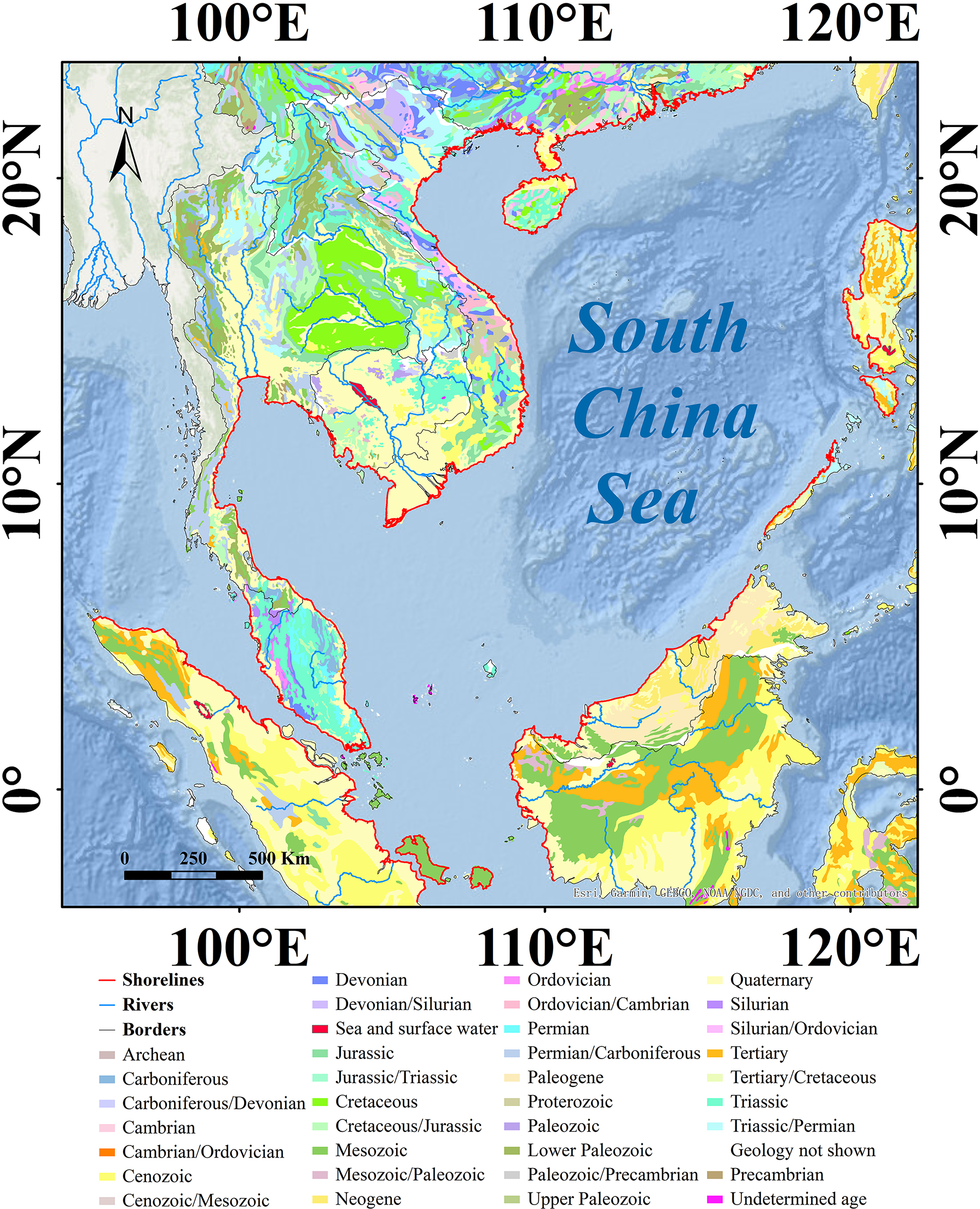
Location map of the study area.
The study area has a mix of tropical rainforest climate, tropical monsoon climate, and tropical savanna climate, with significant precipitation and a monthly average temperature of 18°C or higher (Beck et al., 2018). The low-level wind patterns over the SCS are affected by the orographic features of the surrounding land. In winter, the northeast monsoon prevails in the SCS, with an average wind speed of 10–14 m/s in December, while the southwest monsoon prevails in the summer, with an average wind speed of 6–8 m/s in August (Qiao and Gan, 2012). The sea surface circulation pattern in the SCS is a cyclonic gyre in winter and an anticyclone gyre in summer suggested as being the result of the seasonally reversing monsoon winds.
Tidal waves propagate from the Pacific Ocean into the SCS mainly through the Luzon Strait (Phan et al., 2019). Most areas of the SCS are dominated by mixed, mainly diurnal, tides, but the adjacent areas of the Malay Peninsula are semidiurnal and mixed, mainly semidiurnal (Qiao and Gan, 2012). The tidal amplitude in the central areas of the SCS is usually weaker than that of the shallow coastal zone, such as the Gulf of Tonkin, and the Gulf of Thailand, which reach 7 and 4 m, respectively (Wang and Xie, 2012). Due to the bathymetry of the SCS, the tide current in most sea areas is weak, except for the shallow environments such as the Mekong estuary, Gulf of Tonkin, Gulf of Thailand, and the sea around the Malay Peninsula, where the tide current is stronger, up to about 120 cm/s (Qiao and Gan, 2012). According to the direction of the wave, three wave patterns were defined in the SCS: its prevailing wave direction is NE in winter and autumn and then SE and S in summer; the prevailing wave direction in spring is more complicated, with SE in the north and S in the middle and south. The maxima of the climatological monthly significant wave height in the narrow area from the Luzon Strait to Central Vietnam are high, about 2.5–3.0 m, while those in the southern part of the SCS, Gulf of Thailand, and Gulf of Tonkin are only 0–2 m (Zhai et al., 2021).
Regarding the socioeconomic environment, the SCS is surrounded by countries that have undergone rapid economic and social development since 1980, but the countries’ socioeconomic conditions in the region vary greatly (Bong and Premaratne, 2018). Over the past 40 years, the economies of the countries surrounding the SCS have improved significantly, from 5.4% (1980) to 21.3% (2020) of the world’s GDP (Dataset World Bank, 2022). However, the level of socioeconomic development in these countries varied greatly. China is the biggest developing country, and its economic center, the Guangdong–Hong Kong–Macao Greater Bay Area, is part of the SCS and has the longest shorelines around the SCS. Singapore is a developed city-state that has the highest artificial shoreline rate. Cambodia is one of the least developed countries designated by the United Nations before 2021 (Department of Economic and Social Affairs Economic Analysis, 2021). Indonesia has the lowest artificial shoreline rate and the largest mangrove forest in the world, with the longest mangrove shorelines (Hansen et al., 2013).
Therefore, the diverse natural environment and the different socioeconomic backgrounds have combined to create a rich diversity of shoreline types and distinct development patterns around the SCS. However, the continuous changes in the shoreline characteristics around the whole SCS under anthropogenic influence remain unclear.
Data source
Landsat data are widely used in the research and management of coastal zones due to their long time series, medium spatial–temporal resolution, and global coverage (Wulder et al., 2019). The Landsat data used for this study included 102 scenes of Landsat Multispectral Scanner (MSS) images in 1980, 114 scenes of Landsat Thematic Mapper (TM) images in 1990, 108 scenes of Landsat TM images in 2000, 107 scenes of Landsat TM and Enhanced TM-Plus (ETM+) images in 2010, and 631 scenes of Landsat Operational Land Imager (OLI) images in 2020. All these images were downloaded from the United States Geological Survey (USGS) database and Google Earth Engine (GEE) (Gorelick et al., 2017). To improve the accuracy and assess the uncertainty of the spatial locations and types of shorelines, Google Earth Pro, ESRI (Environmental Systems Research Institute), Bing satellite high-resolution images, and other datasets were also used as references.
Changes in the sea level, temperature, precipitation, ocean wave, storm surge, and other natural factors have significant effects on shoreline erosion and accretion. The artificialization of shorelines is driven by anthropogenic activities, which can be observed in the night light (NTL), impervious surface, and population density. The sea level and storm surge data were derived from Ocean Reanalysis System 5 (ORAS5) and the Global Tide and Surge Reanalysis (GTSR) dataset (Hao et al., 2014; Muis et al., 2016). Due to the impact of storm surges on shorelines being mainly achieved through short periods of sea level rise and ocean wave action, the wave energy can be seen as the index, which can evaluate its impact on shorelines (Mentaschi et al., 2017; Mentaschi et al., 2018). The wave energy density was computed through the ocean wave data from ERA5 (Mentaschi et al., 2017; Hersbach et al., 2020). To assess the energy of the ocean wave, the wave energy density (Pw) is expressed as follows:
where Te denotes the mean wave period and Hs is the significant height of the combined wind waves and swell (Mentaschi et al., 2017; Mentaschi et al., 2018). In addition, temperature and precipitation were also derived from the ERA5 dataset (1980–2020) (Hersbach et al., 2020).
Impervious surface data were selected from the Global Impervious Surface Area (GISA) dataset for the corresponding or adjacent periods (Huang et al., 2022). NTL data were integrated with the Defense Meteorological Satellite Program’s Operational Line Scan System (DMSP-OLS) and Suomi National Polar-Orbiting Partnership Visible Infrared Imaging Radiometer Suite (NPP-VIIRS) dataset on the GEE platform (Small et al., 2005; Li et al., 2013). In addition, datasets from the Global Population Density Grid Time Series Estimates (1980–2000) and UN WPP-Adjusted Population Density (2000–2020) were used as the population data, which covered the past 40 years (Dataset Center for International Earth Science Information Network - CIESIN - Columbia University, 2017). The index of coastline utilization degree (ICUD) was also used to indicate the intensity of the anthropogenic impacts on shorelines (Wu et al., 2014).
Shoreline extraction
MHWL is an ideal shoreline indicator for monitoring long-term shoreline changes. However, it is complicated to obtain enough long-term tide gauge station data to correct the IHWL in a large area such as the SCS. The revisiting time of the Landsat images is 16 or 18 days, and the tidal period is 12 h for the semidiurnal tide around the SCS (Vousdoukas et al., 2020; Bishop-Taylor et al., 2021). Thus, composite images, which were obtained from cloud-free images and processed on the GEE for every stage to remove the short-term variability in the MHWL location over tidal cycles, were adopted in this study.
The shoreline classification system was established based on the substrate types, spatial morphology, and the utilization of shorelines (Figure 2). According to the degree of perturbation, the shorelines were classified into natural and artificial shorelines. Natural shorelines comprise five subclasses, namely, bedrock, sandy, muddy, biological, and river estuary shorelines. Artificial shorelines were also divided into six subclasses according to their utilization type: aquaculture, constructed, reclamation, salt pan, traffic, and wharf dikes.
Figure 2
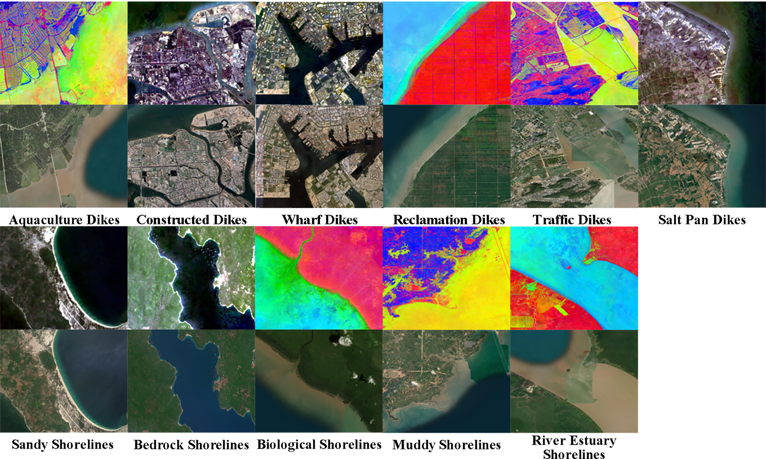
Examples of Landsat and high-resolution satellite images of the different types of shorelines.
Bedrock shorelines are irregular and jagged and are located at the strait of the headland bay coast and rocky coast, and their color depends on the rock type. The location of bedrock shorelines is at the base of the cliff or the inside of the surf zone. Muddy shorelines are relatively straight and have gentle slopes; there are usually some tidal channels on the beach. Muddy shorelines are generally located at the vegetation line. Sandy shorelines are also relatively straight, located at the bay of headland bay coast with beach ridges, and the tone of the sandy beach is bright white or dark, which is affected by the tides. The sandy shoreline location is at the dry/wet line. Biological shorelines are generally distributed on silt flats with weak hydrodynamics and fine substrates, mainly including mangrove and coral reefs. Mangrove shorelines occupy the majority of the biological shorelines around the SCS. Mangrove forests are irregularly shaped and darker than terrestrial vegetation, and the mangrove shoreline location is generally on the landward side of the vegetation patch (Figure 2). According to the utilization, artificial shorelines can be classified into six subclasses, as mentioned above. The width of aquaculture dikes is usually narrow, with water bodies on both sides. Constructed and wharf dikes are both surrounded by large impervious surfaces, with the wharf dikes surrounded by harbor ponds and ships (Figure 2).
Generally, the methods of shoreline extraction can be categorized into three: manual visual interpretation, automatic extraction, and semi-automatic extraction. For automatic and semi-automatic extraction, the shoreline extraction can be treated as edge detection or classification problem, with the characteristics of higher efficiency and lower accuracy compared with manual visual interpretation (Bishop-Taylor et al., 2021). Thus, manual visual interpretation was used, which is the most reliable shoreline extraction method applied to identify shoreline locations and types. According to the degree of shoreline curvature, points with appropriate sparsity, which are on the MHWL image pixel, were considered as shorelines. Then, the length of the shoreline was calculated using ArcGIS with a scale of 1:10,000 under the EPSG:32651 projected coordinate system. Using composite images and the normalized difference water index (NDWI), normalized difference vegetation index (NDVI), and normalized difference built-up index (NDBI) combined with high-resolution images, Open Street Map, Google Street View, geology map, fieldwork reports, and other data, the shorelines in 2020 were first extracted and established corresponding to the interpretation standards on remote sensing images (Rokni et al., 2014; Ke et al., 2015; Guha et al., 2018) (Figure 3). Subsequently, these standards were used to identify the locations and the types of shorelines in the other stages.
Figure 3
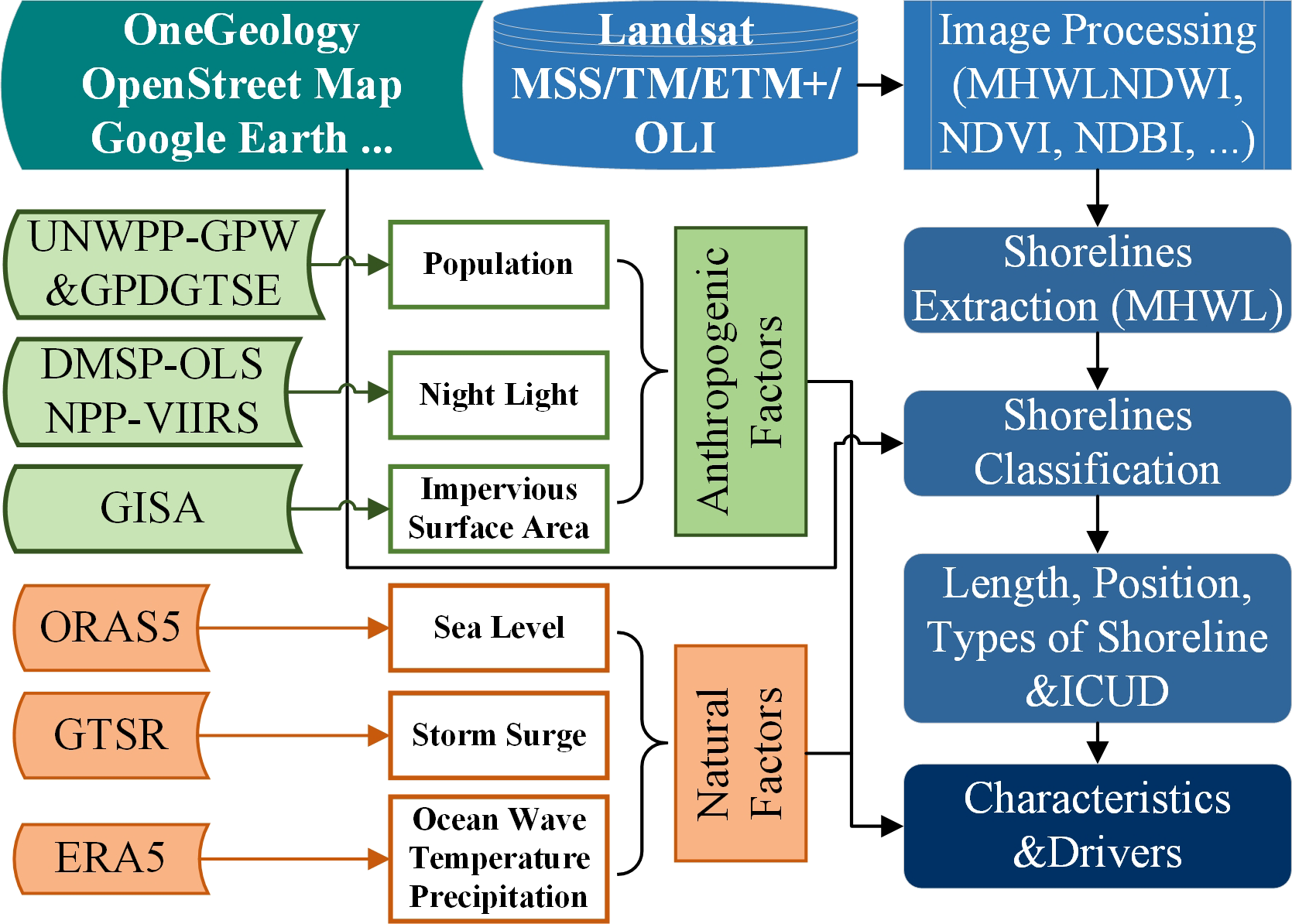
Workflow of the study. GISA, Global Impervious Surface Area; DMSP-OLS, Defense Meteorological Satellite Program’s Operational Line Scan System; NPP-VIIRS, National Polar-Orbiting Partnership Visible Infrared Imaging Radiometer Suite; ORAS5, Ocean Reanalysis System 5; GTSR, Global Tide and Surge Reanalysis; MSS, Multispectral Scanner; TM, Thematic Mapper; ETM+, Enhanced TM-Plus; OLI, Operational Land Imager; MHWL, mean high water line; NDWI, normalized difference water index; NDVI, normalized difference vegetation index; NDBI, normalized difference built-up index; ICUD, index of coastline utilization degree.
Accuracy verification
The uncertainties in the estimation of the shoreline locations can be roughly divided into two types: positional and measurement uncertainties. Positional uncertainties are related to the features and phenomena that reduce the precision and accuracy of the shoreline position, such as seasonal error, tidal fluctuation, and ocean waves (Mondal et al., 2021). On the other hand, the measurement uncertainties are usually related to pixel, geometric, and terrain errors, among others. Most of the factors in the positional uncertainties can be minimized as much as possible by synthesizing multiple images of different seasons and tides. In addition, we focused on long-term shoreline changes and the positional uncertainties due to short-term random factors such as seasonal error, tidal fluctuation, and ocean waves having limited impact on the study. Regarding measurement uncertainties, the original satellite images were from the USGS Level 2 Landsat surface reflectance production in GEE, with the good and consistent effect of geometric correction, terrain correction, and alignment. Thus, the accuracy of a shoreline location is mainly related to the pixel error, which depends on the spatial resolution of remote sensing images. One hundred sample points were generated using a random sampling method for shorelines of each stage, these points were imported into Google Earth Pro, and then high-resolution satellite images of the corresponding time were selected to obtain the accurate location of the verification points on the shoreline. The uncertainty of shoreline location can be measured using the distance between the sample points and the corresponding validation points (Zhang et al., 2021). The whole average error of shoreline location was 21.8 m and the standard deviation (SD) was 20.2 m, both less than the theoretical maximum permissible error (TMPE) (Zhang et al., 2021). In addition, the average error and SD of each stage were both less than those of the TMPE. The accuracy of shoreline type was also assessed through the same sample points and the corresponding validation points; the confusion matrix showed that the overall accuracy was 89.6% and the kappa coefficient was 0.871. Therefore, the accuracies of shoreline type and location are acceptable for this study.
Regarding the applicability of the auxiliary dataset, sea level data were from ORAS5, which are reconstructed and analyzed data generated by the model to overcome the deficiency of satellite altimetry data in time (1993 to the present) and the uneven distribution of tide gauge stations in the SCS with different data (Hao et al., 2014). By comparing these with the data from the tide gauge stations in Manila and other places, the ORAS5 data were found acceptable to reflect the decadal variability of the sea level (Hao et al., 2018; Han et al., 2019). Most of root mean square error of GTSR sea level across the validation sites in the SCS was lower than 0.2 m. Moreover, the correlation coefficient between GTSR sea level and the observed daily maximum sea level was higher than 0.8 (Muis et al., 2016). Compared to the observational data, the wave parameters, such as Hs and Te, provided by ERA5 showed high accuracy in the SCS, and the correlation coefficient of Hs was in the range of 0.87–0.93 (Liu et al., 2022). Regarding temperature and precipitation, ERA5 is also a widely used climate reanalysis dataset with 0.1 degree spatial resolution, spanning the period from 1950 to the present in the study of Southeast Asia and southern China. It can capture the annual patterns of observed precipitation in southern China well, with correlation coefficient values ranging from 0.796 to 0.945 (Jiao et al., 2021). The correlation coefficient between the ERA5 monthly temperature and weather station data ranged from 0.98 to 0.99 (Li, 2020; Hamed et al., 2022; Zou et al., 2022).
Digital shoreline analysis system
The DSAS is a software extension developed by USGS and works with ArcGIS (Himmelstoss et al., 2018). DSAS can generate transects from the baseline at regular intervals and ensures that each transect has intersected points with the shoreline vector. The distance from the baseline to the time series of shoreline data along the transect was used to calculate the rate-of-change statistic. The regular interval was 300 m and generated 91,510 transects in the study. The intersect multipoint, which was from the same transect, can obtain attributes from the corresponding shoreline data and represent the change of shorelines. Thus, the shoreline utilization type can be denoted as a transfer matrix disregarding changes in shoreline location.
Influencing factors
The decadal net shoreline movement (NSM) can be calculated by measuring the difference between the length from baseline to shorelines of adjacent times along the transect. On the other hand, the nearest natural factor data point to the transect is considered the natural factor that influences the shoreline at the transect location. Similar to the NSM, the difference between the natural factors of adjacent times can be calculated as the decadal net natural factor change (NNFC). Thus, there were four sets of each transect consisting of the NSM and NNFC (ocean wave, sea surface height, storm surge, temperature, and precipitation), which were calculated from the five-stage shoreline and natural factor datasets. All of the above datasets were first z-standardized, and then the bivariate correlations between all NSMs and each NNFC of adjacent times were calculated; finally, the overall correlation between NSM and NNFC was evaluated using multiple correlation analysis.
The density of NTL, the GISA, and the population were calculated by dividing the total values of NTL, GISA, and population by the area of each province. Corresponding to shoreline data, there were five sets of each province consisting of the ICUD; the percentages of natural shorelines, constructed dikes, and wharf dikes; the density of NTL, GISA, and population. All of these data were also z-standardized, and then the bivariate correlations between the index of shorelines and the anthropogenic activities were calculated.
Results
The length changes of shorelines
The shoreline around the SCS has increased by nearly 1,000 km, from 28,168.9 (1980) to 29,164.4 km (2020), which maintained continuous growth during the past 40 years, with the most rapid growth being in the 1990s (Table 1).
Table 1
| Countries | 1980 | 1990 | 2000 | 2010 | 2020 |
|---|---|---|---|---|---|
| China | 6,408.0 | 6,689.6 | 6,812.1 | 6,834.8 | 7,117.9 |
| Vietnam | 4,455.7 | 4,452.3 | 4,552.8 | 4,567.2 | 4,542.8 |
| Cambodia | 733.0 | 723.8 | 734.8 | 720.4 | 613.0 |
| Thailand | 2,338.5 | 2,325.5 | 2,438.7 | 2,513.2 | 2,455.3 |
| Malaysia | 4,219.9 | 4,167.4 | 4,343.7 | 4,324.2 | 4,234.6 |
| Indonesia | 5,798.7 | 5,635.7 | 5,764.7 | 5,784.9 | 5,830.8 |
| Singapore | 205.8 | 218.9 | 243.7 | 261.1 | 327.9 |
| Brunei | 197.3 | 201.0 | 222.5 | 218.6 | 220.9 |
| Philippines | 3,812.0 | 3,829.6 | 3,865.6 | 3,770.9 | 3,821.2 |
| South China Sea | 28,168.9 | 28,243.8 | 28,978.6 | 28,995.3 | 29,164.4 |
Length of shorelines by countries (in kilometers).
The changes of shorelines in most countries were consistent with the trend of the whole SCS, especially in China and Singapore (Table 1). These two countries had the most significant growth in shorelines. China, attributed with the longest shoreline around the SCS, contributed 71.3% (approx. 710.0 km) of the overall SCS shoreline growth. Singapore had the highest percentage of shoreline growth among all countries around the SCS, about 60% (approx. 122.0 km). Similar to Singapore, another country that had more than 10% (approx. 23.6 km) shoreline growth is Brunei, which had shorter shorelines of only about 200 km. The increases of shorelines in Thailand and Vietnam were 116.8 and 87.1 km, respectively, accounting for 11.7% and 8.8% of the overall SCS shoreline growth. Moreover, Cambodia was the only country that has seen a decrease in shorelines. In addition, changes in the shoreline length in the remaining countries (Malaysia, Indonesia, and the Philippines) were relatively low, less than 1%.
The ICUD of the provinces around the SCS showed a continuous growth trend, with that of Guangdong, Bangkok, Singapore, Kuala Lumpur, and Manila particularly obvious, indicating that the anthropogenic activities and exploitation intensity of the shorelines around the SCS had been increasing stage by stage (Figure 4).
Figure 4
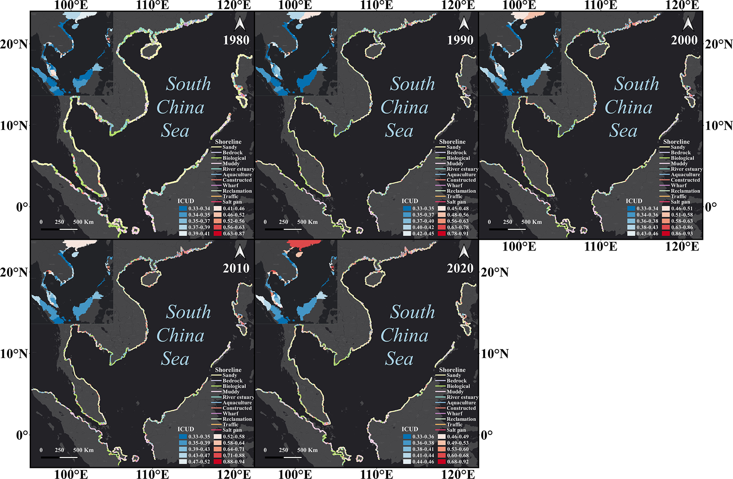
Index of coastline utilization degree (ICUD) of provinces and the types of shoreline evolution around the South China Sea (SCS).
In Singapore, the length of the shorelines increased by 122.1 km, from 205.8 (1980) to 327.9 km (2020), which is almost 60% of the total shorelines, and the period of the most rapid shoreline growth has been the last 10 years (Table 1). This growth has been achieved generally through nearshore engineering and reclamation (Figure 5A). The length of Brunei’s shorelines also increased by 12.0%, from 197.3 (1980) to 221.0 km (2020), with nearshore engineering and wharf embankment also playing a significant role in the shoreline growth (Figure 5B).
Figure 5
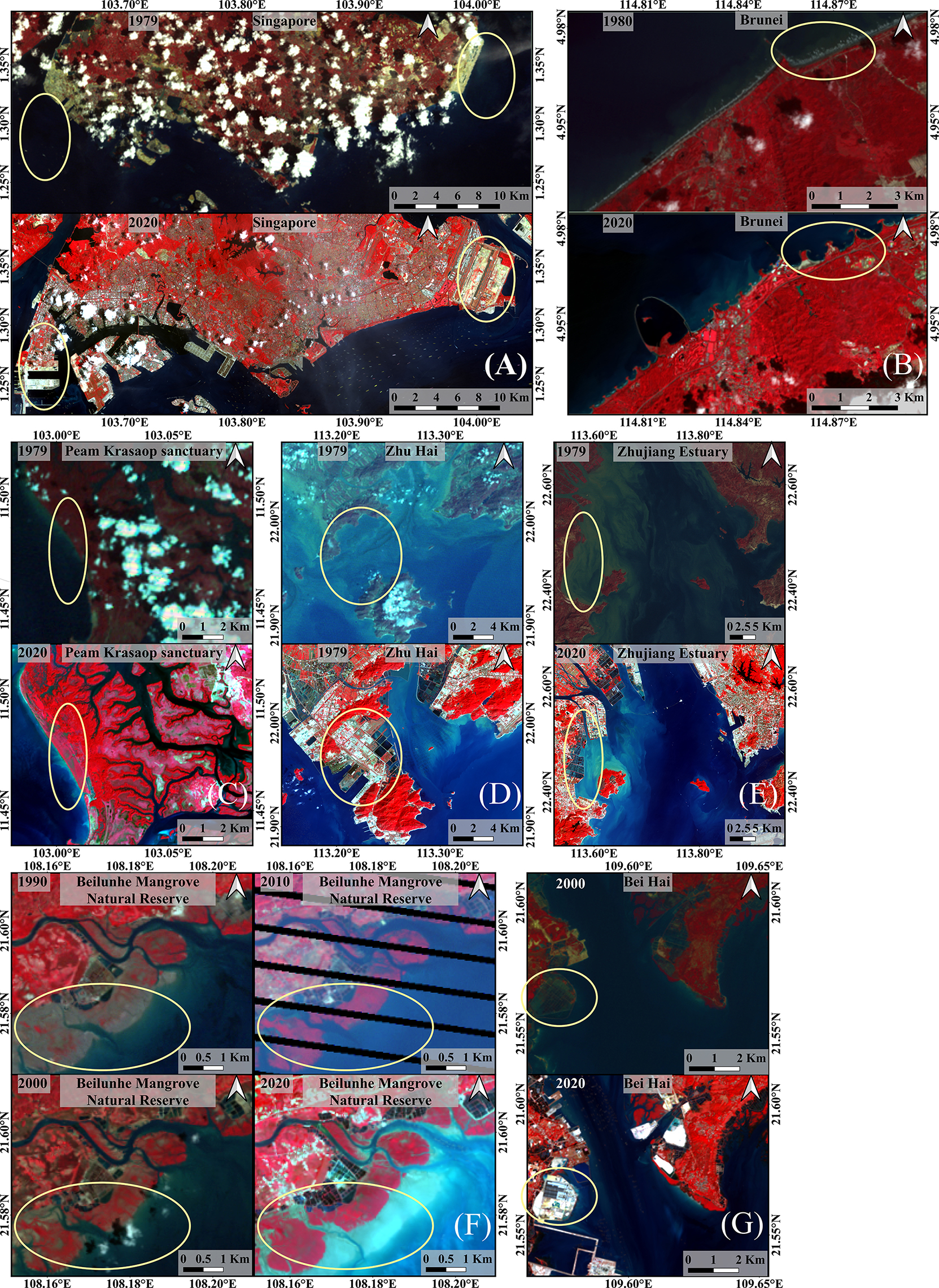
Anthropogenic activities on different shorelines. Nearshore engineering, wharf embankment and reclamation in Singapore, Brunei (A, B). Growth of the mangrove forest in Cambodia (C). Reclamation engineering connecting nearshore islands to the mainland in Guangdong. (D, E) Growth of mangrove forest in Guangxi (F). Conversion of aquaculture dikes into constructed dikes (G).
In China, the length of shorelines increased by 11% (approx. 710.0 km) over the past 40 years, with the major growth occurring in the 1990s and during the last decade (Table 1). Guangdong increased by 417.2 km, from 3,337.3 (1980) to 3,754.5 km (2020), accounting for approximately 58% of the SCS shoreline growth. The provinces of Guangxi and Hainan also increased by about 141 km, but the shoreline lengths of these provinces were 1,307.3 and 1,597.3 km, respectively (Figure 4). Changes in the shoreline length in Hong Kong and Macao had relatively small impacts on the whole SCS shorelines due to them being shorter.
The length of Cambodia’s shorelines decreased by nearly 120 km during the past 40 years, and the highest decrease occurred in the Peam Krasaop Wildlife Sanctuary, which is a protected area located in southwestern Cambodia. Despite the impact of anthropogenic activities on the shoreline of this sanctuary, the mangrove forests were still relatively well protected, with little increase toward the sea since 1993, when this sanctuary was established. This growth of the mangrove forest led to the truncation of the mangrove shorelines, resulting in a reduction in shoreline length (Figure 5C).
The utilization types of shorelines
Artificialization was the most prominent feature of the shorelines around the SCS over the past 40 years. The natural shorelines declined from 26,026.0 (1980) to 21,377.0 km (2020), with a percentage decrease from 92.4% to 73.3%. At the same time, artificial shorelines showed a more than twofold increase from 2,143.1 (1980) to 7,787.3 km (2020) (Figure 6). The increase of artificial shorelines was due not only to the artificialization of natural shorelines but also to nearshore engineering and reclamation (Figures 5B, D). The proportions of artificial shorelines varied greatly from country to country, from city-states like Singapore to countries with long and diverse shorelines like China. In 2020, the highest shoreline artificiality rate of 77.6% was in Singapore, while the lowest, which was 9.6%, was in Indonesia.
Figure 6
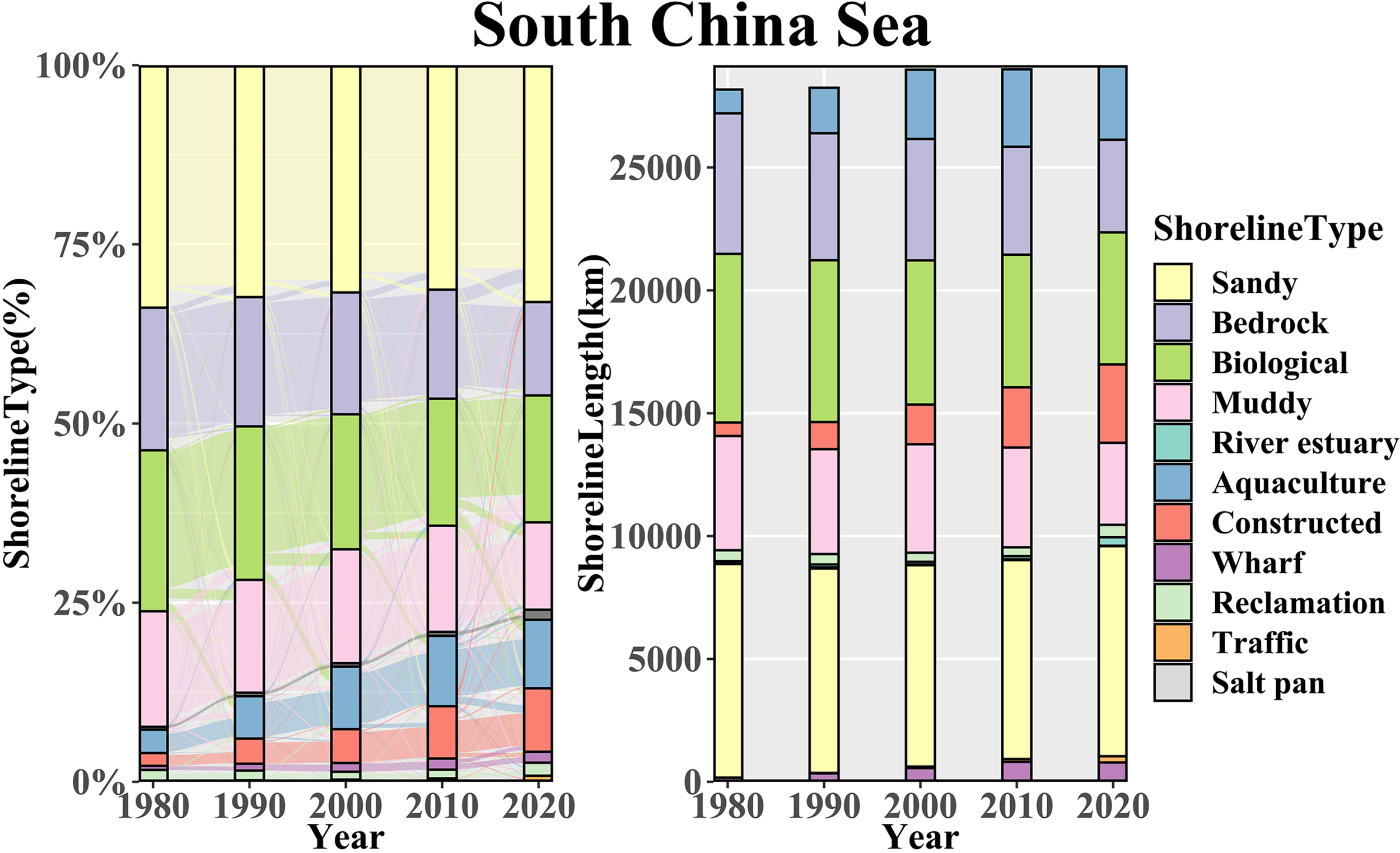
Sankey map and lengths of the different shorelines around the South China Sea (SCS).
In China, natural shorelines decreased from 5,490.9 (1980) to 3,259.4 km (2020), with a percentage decline from 85.7% to 45.8% accordingly. Among natural shorelines, bedrock and mangrove shorelines declined most significantly, with their lengths declining by 49.3% and 65.7%, respectively. For artificial shorelines, the growth of aquaculture dikes occurred mainly before 2000, while the growth rate of constructed dikes remained largely stable, with only a slight increase in the last decade. Regarding the source of new artificial shorelines, aquaculture dikes generally developed from mangrove shorelines and some muddy shorelines, and more than 10% of mangrove shorelines were reclaimed for aquaculture dikes every decade. Unlike aquaculture dikes, which usually developed from natural shorelines, the newly constructed dikes developed from a variety of sources, including natural shorelines such as sandy and bedrock shorelines, as well as from conversions of aquaculture and reclamation dikes, with the proportions of shorelines developed from natural shorelines gradually decreasing from 84.0% (1980) to 44.2% in the last decade. In addition, the growth of the wharf dikes was significant, from 13.5 (1980) to 388.1 km (2020), even though it represented only 5.5% of the total shorelines in 2020. The main growth period of wharf dikes was before 2010, with an average annual growth rate of more than 10%.
The percentage of Vietnamese natural shorelines declined from 91.4% (1980) to 76.0% (2020), reducing the length of natural shorelines by 623.4 km; on the other hand, artificial shorelines increased from 382.0 to 1,092.5 km. According to shoreline type, Vietnamese natural shorelines can be divided into three parts: mangrove and muddy shorelines along the Gulf of Tonkin, bedrock and sandy shorelines in the central part, and mangrove and muddy shorelines in the Mekong River Delta (Figure 4). Vietnamese artificial shorelines were also dominated by aquaculture and constructed dikes, which occupied 11.1% and 9.7% of the total shorelines in 2020, respectively. Moreover, they were mainly distributed in economically developed areas such as Hanoi and Ho Chi Minh City. All types of natural shorelines in Vietnam declined to varying degrees, especially the mangrove shorelines which decreased from 1,456.5 (1980) to 1,129.6 km (2020), accounting for 24.9% of the total shorelines in 2020, down from 32.7% (1980). The growth of artificial shorelines was dominated by constructed and aquaculture dikes, which increased by nearly eight times and 54.3% in four decades, respectively. The growth of aquaculture dikes occurred mainly before 2000, especially in the 1980s, with an increase of 73.9%. More than 60% of the new aquaculture dikes developed from mangrove shorelines, with some from muddy shorelines.
Compared with Vietnam, the percentage of artificial shorelines in Thailand was lower, at 21.6%. Most of the natural shorelines were sandy shorelines, with small proportions of bedrock and mangrove shorelines. The sandy and bedrock shorelines were generally located in the east of the Malay Peninsula, while most of the mangrove shorelines were in the north of Bangkok Bay. The artificial shorelines were mostly aquaculture and constructed dikes located in the eastern and northern parts of Bangkok Bay (Figure 4). The proportion of natural shorelines decreased from 93.9% (1980) to 78.4% (2020), chiefly due to the bedrock and mangrove shorelines being developed into aquaculture and constructed dikes. The proportion of artificial shorelines in Cambodia was also low, only 17.4% in 2020, with the mangrove shorelines accounting for more than 40% of the overall shorelines, generally in the bays and estuaries; the artificial shorelines were aquaculture and constructed dikes, which were concentrated near Sihanoukville (Figure 4).
Singapore had the highest proportion of artificial shorelines around the SCS, with only a small amount of sandy and bedrock shorelines, which was in conformity with its role in world maritime logistics. Most of the bedrock and mangrove shorelines developed as constructed and wharf dikes in the 1980s. Apart from the development of natural shorelines, Singapore’s artificial shorelines developed from reclamation and outlying island engineering (Figure 5A). The growth of constructed dikes remained relatively stable at a rate of more than 50%, except in the 2000s. The growth of wharf dikes, on the other hand, mainly occurred in the 1980s and had been growing modestly since then. As the country with the shortest shoreline around the SCS, Brunei’s shorelines were relatively homogeneous, consisting of over 58.1% sandy shorelines, 23.5% mangrove shorelines, and 10.6% constructed dikes. Sandy and mangrove shorelines were mainly along the western shorelines facing the open sea and the Brunei Bay, respectively, and the constructed dikes were in the capital city of Bandar Seri Begawan (Figure 4).
Indonesia was second only to China in terms of shoreline length around the SCS, with the lowest percentage (9.6%) of artificial shorelines in 2020, which were chiefly aquaculture, reclamation, and constructed dikes. Indonesia is located in the tropics, and most of its shorelines have weak hydrodynamic environments, with extensive muddy and mangrove shorelines accounting for 39.1% and 27.5%, respectively, and only a number of sandy shorelines (17.9%) distributed in the northern part of Sumatra Island, Bangka Island, and Belitung Island (Figure 4). The sandy and bedrock shorelines in Indonesia had not changed much in the past 40 years. On the other hand, the muddy and mangrove shorelines had been widely developed as artificial shorelines. The development of the aquaculture dikes occurred mainly between 1990 and 2010, from 33.1 (1990) to 209.7 km (2010), with their proportion increasing from 0.6% to 3.6%. Unlike in other countries, most of the new aquaculture dikes in Indonesia developed from sandy shorelines, with muddy and mangrove shorelines accounting for only about 23%. The increase in constructed dikes (from 97.1 to 165.6 km) occurred between 2000 and 2010, generally from the development of muddy and mangrove shorelines around the city. In addition, the percentage of reclamation dikes also increased after 2000, accounting for more than 3.0% (approx. 176.1 km) in 2020, with more than 70% of the new reclamation dikes reclaimed from muddy shorelines (Figure 4).
Malaysia’s artificial shorelines had grown from 210.8 (1980) to 753.8 km (2020), increasing from 5% to 17.8% of the overall shorelines. The natural shorelines consisted of sandy and mangrove shorelines, with the sandy shorelines chiefly located in the eastern part of the Malay Peninsula and the part of Kalimantan Island facing the open ocean and the mangrove shorelines mostly located in the western part of the Malay Peninsula and around the bays in Kalimantan Island (Figure 4). The artificial shorelines were mainly constructed dikes, located in the western and southern parts of the Malay Peninsula, which had gradually increased from 144.3 (1980) to 450.3 km (2020), with the growth rate being over 40% per decade until 2010. The new constructed dikes were generally developed from the natural shorelines, with muddy and sandy shorelines being the mainstay.
The location change of shorelines
According to the whole average error of shoreline location and the SD, stable shorelines can be defined as the shoreline with NSM less than ±42 m. Naturally, advancing shorelines have NSM greater than 42 m, and the NSM of retreating shorelines was less than −42 m. More than 40% (approx. 12,000 km) of shorelines had been stable during the last 40 years, with an average NSM of 0.52 m. About 28% (approx. 6,800 km) of the shorelines showed a landward retreat, with an average NSM of −175.6 m. The distribution of the retreating shorelines was spatially homogeneous, and most were sandy and muddy shorelines. About 30% (approx. 6,800 km) of the shorelines showed a seaward advance, with the average NSM being 633.5 m. Most of the advancing shorelines were concentrated in areas with high anthropogenic activities, such as the Greater Bay Area, the Gulf of Tonkin, Bangkok Bay, Singapore, and Manila. In terms of shoreline type, most of the advancing shorelines were artificial shorelines such as constructed, aquaculture, and wharf dikes.
The overall trend of the SCS shorelines was seaward, showing an average end point rate (EPR) of 4.4 m/year, with 2% of the EPRs being less than −10 m/year, 26.5% between −10 and −1 m/year, 37.6% between −1 and 1 m/year, 20.2% between 1 and 5 m/year, 5.7% between 5 and 10 m/year, and 10% of the EPRs being greater than 10 m/year. There were significant differences in the EPRs between the different shoreline transformation types (p< 0.05). The EPRs of shorelines larger than 10 m/year were generally located in the Greater Bay Area, Gulf of Tonkin, Singapore, Manila, and other cities (Figure 7). The most rapid advance of shorelines to the sea occurred in Guangdong Province in the 1980s, which was due to reclamation engineering connecting nearshore islands to the mainland (Figure 5E). The EPRs of the sandy, bedrock, and muddy shorelines were −2.31, 0.43, and −1.07 m/year between 1980 and 2020, respectively.
Figure 7
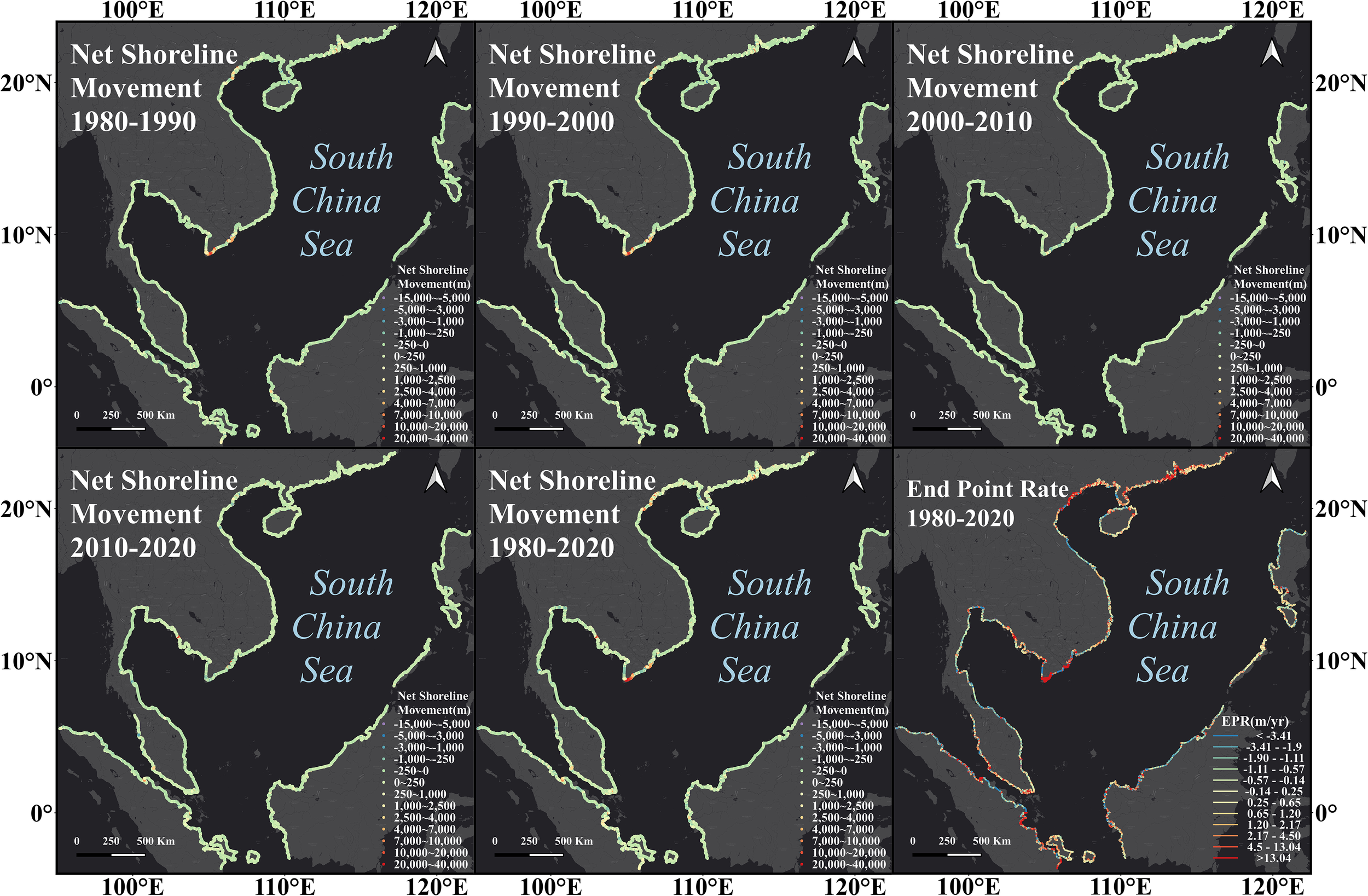
Net shoreline movement (NSM) and end point rate (EPR) map of the South China Sea (SCS) between 1980 and 2020.
In the 1980s, most of the sandy shorelines retreated, with an EPR of −2.08 m/year. Of the mangrove shorelines, 84.4% retained their type, but their average EPR was 11.59 m/year seaward, indicating that although the shoreline type did not change, the survival space of mangrove forests was more severely compressed. Muddy shorelines also had a minor retreat, with an EPR of −1.2 m/year. In addition, the new artificial shorelines were mainly aquaculture and constructed dikes, of which the aquaculture dikes developed from mangrove, muddy, and bedrock shorelines, with EPRs of 112.31, 11.17, and 10.61 m/year, respectively. The new constructed dikes generally developed from sandy and bedrock shorelines. In the process of developing into constructed dikes, sandy shorelines retreated with an EPR of −2.48 m/year, but bedrock shorelines had a greater seaward EPR of 8.24 m/year due to their stability and development pattern (Figure 8).
Figure 8
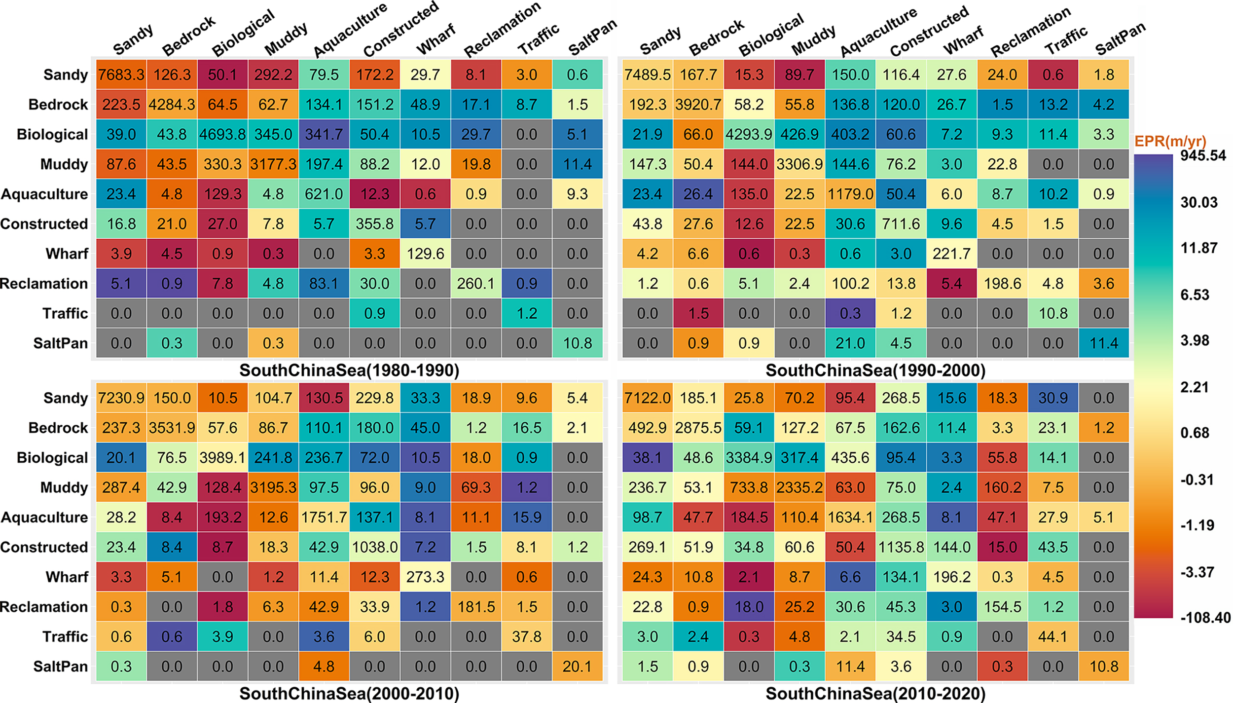
Transfer matrix (in kilometers) of shoreline types with end point rates (EPRs) around the South China Sea (SCS).
In the 1990s, the sandy, bedrock, and muddy shorelines remained relatively stable, with EPRs of 0.73, 0.17, and 1.12 m/year, respectively, while the mangrove shorelines were still retreating, with an EPR of 5.66 m/year, meaning that its survival space continued to be compressed (Figure 8). The new artificial shorelines were still mainly aquaculture and constructed dikes, with most constructed dikes from the development of sandy and bedrock shorelines, with EPRs of 3.55 and 15.57 m/year, respectively, while the aquaculture dikes developed from various sources: mangrove (403.2 km), sandy (150.0 km), muddy (144.6 km), and bedrock (120.0 km) shorelines.
In the 2000s, the spatial location of the natural shorelines remained largely unchanged, and the EPR of the mangrove shorelines was 1.6 m/year, which was still being exploited, but at a significantly constrained rate (Figure 8). The types of the new artificial shorelines still included aquaculture and constructed dikes, but the increase in constructed dikes (767.1 km) exceeded that of aquaculture dikes (680.4 km) for the first time. Similar to that in the previous two decades, the increase of aquaculture dikes was also from the development of natural shorelines, mainly mangrove, sandy, and bedrock shorelines, with EPRs of 15.3, −5.96, and 11.65 m/year, respectively. Of the newly constructed dikes, 75.8% developed from sandy and bedrock shorelines. At the same time, 24.2% of the newly constructed dikes were converted from aquaculture, reclamation dikes, and other artificial shorelines. In the process of developing into constructed dikes, the change in shoreline location due to the exploitation of sandy shorelines was not significant, with an EPR of 0.97 m/year, that of bedrock shorelines was 8.68 m/year, and the EPR of the conversion from aquaculture dikes was 1.1 m/year.
The spatial locations of the sandy, bedrock, and muddy shorelines also did not change much during the last decades, and their EPRs were −0.65, 1.12, and −0.86 m/year, respectively, while the EPR of mangrove shorelines reached 5.9 m/year, highlighting the continuous pressure on mangrove survival (Figure 8). Among the new artificial shorelines, the proportion of constructed dikes (1,087.5 km) again exceeded that of aquaculture dikes (762.6 km), with EPRs of 7.51 and 1.52 m/year, respectively.
Correlation analysis
The correlation coefficients between the NSM and NNFC of ocean wave density, precipitation, temperature, sea surface height, and sea surface height due to surge were 0.008, 0.021, 0.011, 0.022, and 0.048, respectively. The multiple correlation coefficient between the NSM and all NNFC was only 0.063. In contrast to natural factors, there were some higher correlation coefficients between the indexes of shoreline types and human activities, especially the ICUD and the percentage of constructed dikes (Table 2).
Table 2
| Density | |||||
|---|---|---|---|---|---|
| NTL | GISA | Population | |||
| ICUD | 0.764 | 0.740 | 0.659 | ||
| Percentage | Natural shorelines | −0.451 | −0.594 | −0.489 | |
| Constructed dikes | 0.736 | 0.636 | 0.644 | ||
| Wharf dikes | 0.568 | 0.715 | 0.550 | ||
Correlation coefficients between the index of shorelines and anthropogenic activities (p< 0.01).
NTL, night light; GISA, Global Impervious Surface Area; ICUD, index of coastline utilization degree.
Discussion
Change of shoreline type
Natural shorelines
Over the past 40 years, 34.3% (about 9,800 km) of the SCS shoreline types had changed, with nearly 90% of the changes occurring in natural shorelines. Most of the changes in natural shorelines had been dominated by anthropogenic activities, with different development approaches and strategies for different natural shorelines. More than half of the developed sandy shorelines were used as constructed dikes and 31.0% as aquaculture dikes. Bedrock shorelines developed in a similar manner to sandy shorelines, with most of them also developed as constructed dikes and one-third as aquaculture dikes. The development of mangrove shorelines was covered by aquaculture, constructed, and reclamation dikes, with more than 61.4% of the exploited mangrove shorelines being aquaculture dikes and 24.7% as constructed dikes.
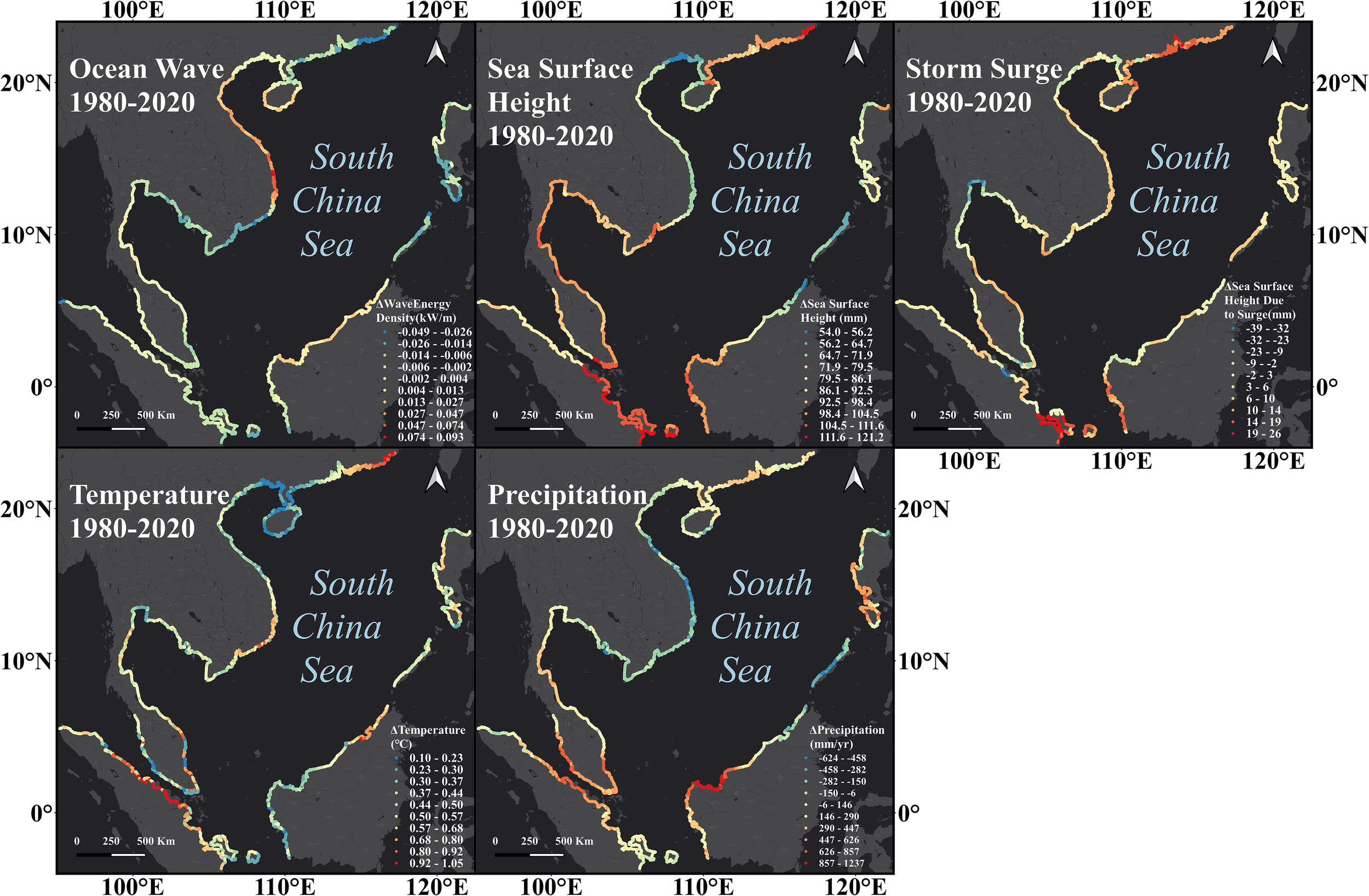
Except for the development of artificial shorelines, the proportion of unchanged natural shoreline types was over 82.3%. Most of the shorelines with changing types were located in areas of high-intensity anthropogenic activity, such as the Greater Bay Area, the Gulf of Tonkin, Ho Chi Minh City, Bangkok, Singapore, Kuala Lumpur, and Manila (Figure 4). However, the areas where natural factors changed significantly differed; for example, wave energy changed significantly in Central Vietnam, sea level changed significantly in the north and south of the SCS, and the precipitation and temperature changes primarily occurred in northeast Sumatra and Central Kalimantan (Figure 9). This means that, in the long process of topographic and geomorphological evolution, most shorelines have reached a dynamic balance with the surrounding environment and kept their types relatively unchanged at decadal scales (Stive et al., 2002). Thus, the spatial mismatch between areas with changing shoreline types and that of natural factors indicates that most natural shorelines can maintain their types and were less affected by the change in sea level, ocean waves, precipitation, and temperature without the influence of anthropogenic activities.
Figure 9
Evolution of natural factors around the South China Sea (SCS).
Therefore, since natural shorelines remain relatively stable without human influence, the most prominent characteristic of the shoreline types around the SCS is artificialization. Different natural shoreline types were subjected to different development patterns, generally depending on the original shoreline types, socioeconomic environment, the policies of the regions, and other factors. In addition, the impact of anthropogenic activity was not only on the exploitation of natural shorelines but also on the protection of natural shorelines through nearshore engineering and protected areas (Jia et al., 2018; Jianing et al., 2019; Veettil et al., 2020; Latif and Yong, 2021). For instance, the Beilunhe Mangrove Natural Reserve was first established as a county mangrove reserve in 1985, then became a provincial marine nature reserve in 1990, and finally a national reserve in 1999. With the improvement in reserve level, the area and shoreline length of the mangrove forest maintained sustained growth (Chen et al., 2009) (Figure 5F).
Artificial shorelines
For artificial shorelines, the development pattern varied over time. Taking the whole SCS as an example, the development of the aquaculture dikes was mainly before 2010, while that of the constructed dikes was growing continuously, and the significant increase in wharf dikes occurred after 1990. Additionally, in the 1980s, there was little conversion between the different utilization types of artificial shorelines, accounting for only about 2%, while in the 2010s, the utilization type of the conversion of artificial shorelines was about 14.7%, generally from aquaculture dikes to constructed dikes and some wharf dikes.
For aquaculture dikes, the production and area of coastal aquaculture ponds in Southeast Asia maintained a sustained growth from 1990 to 2015 with two expansion patterns: outlying expansion from 1990 to 2000 and infilling after 2000. Infilling meant a lower increase in length for the same area, which was consistent with the major growth periods of the length of aquaculture dikes (Luo et al., 2022). The development priorities of different countries also varied. The peak development of aquaculture dikes in most countries around the SCS was consistent with that of the whole SCS, all before 2010, but the development process of the aquaculture dikes in Cambodia was significantly behind that of the whole SCS, peaking around 2010, with the rapid increase of brackish water and marine aquaculture production (Zhe et al., 2020; Dataset Statistics Team of the FAO Fisheries and Aquaculture Division, 2021). Regarding the constructed and wharf dikes, their expansions were closely related to the economic and industrial structure of each country. With the exception of countries like Singapore and Brunei, which have short shorelines and extremely high urbanization rates in the 1980s, urbanization and constructed dikes continued to grow in most countries during the four decades (Dataset World Bank, 2022). The maritime logistics in China and the Southeast Asian countries saw rapid growth after 1990, which coincided with the expansion of shipping infrastructure such as wharves and ports (Salim et al., 2017; Dataset UNCTADstat, 2020). For example, the Zhujiang River Estuary had been one of the most important economic engines around the SCS since the Chinese reform and opening up in 1978, with dramatic changes on the shoreline driven by anthropogenic activities (Ai et al., 2019) (Figure 5E). In contrast to China, where the percentage of constructed dikes was typically more than three times that of wharf dikes, Singapore’s constructed dikes were far fewer than wharf dikes, revealing the very different industrial structures and shoreline development patterns in these two regions (Glaser et al., 1991; Lai et al., 2015).
Regarding the source of new artificial shorelines, the ratio of development from natural shorelines to converted from other artificial shorelines continued to decrease. The ratios around the SCS were 9.3 (1980) and 1.8 (2020), and the ratios in China, Philippines, Vietnam, and Singapore were 1.4, 1.6, 1.5, and 0.1 in 2020, respectively, lower than that of the whole SCS in both time points. This means that the shoreline development in these countries had shifted from the increment stage to both inventory and increment stages, while other countries were still focused on developing natural shorelines.
Therefore, the development priorities of countries in different periods were consistent with their socioeconomic states at the corresponding time, and these factors not only influenced the exploitation of natural shorelines but also had a significant impact on the transformation between artificial shorelines of different utilization types.
The change of shoreline location
Natural processes
The most seaward advance of the SCS shorelines was distributed in China, northern Vietnam, Singapore, and other areas where human impact was intense, while the landward retreat was mainly spatially homogeneous and most were sandy and muddy shorelines (Luijendijk et al., 2018) (Figure 7). The change in spatial location with utilization type transformation was significant compared with that of the shorelines that maintained their types (Figures 7 and 8). The EPRs of sandy, bedrock, and muddy shorelines were −2.31, 0.43, and −1.07 m/year, respectively, while the average EPRs on the artificialization process of aquaculture, constructed, and wharf dikes were 26.3, 27.8, and 34.0 m/year, respectively.
The geological structures and the topography of coastal zones both determine the shoreline type, stability, and evolution; climate and the ocean environment also have a significant influence (Sérgio et al., 2000; Zhang et al., 2021). Bedrock shorelines, which are generally located at the base of bluff or cape of a headland bay, are more stable than other natural shorelines, which are usually distributed in bays, flatlands, and other environments with weak hydrodynamics (Zhang et al., 2021). Compared with bedrock shorelines, the sandy, mangrove, and muddy shorelines are more sensitive and vulnerable to sea level rise and storm surges, and mangrove shorelines are also affected by meteorological variables (Luijendijk et al., 2018; Sippo et al., 2018; Zhang et al., 2021). Thus, a lot of natural factors can influence the location of shorelines, such as the sea level, storm surges, and sediment supply (Le Cozannet et al., 2014; Spencer et al., 2015; Luijendijk et al., 2018; Sippo et al., 2018; Besset et al., 2019; Vousdoukas et al., 2020). Mangrove shorelines are affected not only by these factors but also by the temperature and precipitation, which are important for mangrove forests (Adame and Lovelock, 2011).
The wave energy density around the SCS has not changed a lot during the past 40 years, but showing a significant increase in Central Vietnam (Figure 9). There had been a general rise of sea level in the SCS, but this rise had been largely uniform and showed little relation to the location change of shorelines (Figure 9). In addition, the correlation coefficient between the NSM and NNFC was lower than 0.1. In general, bedrock shorelines have the strongest hydrodynamic environment, followed by sandy shorelines, with the muddy and mangrove shorelines having the weakest. The weaker stability of sandy shorelines and the relatively stronger hydrodynamic environment together created a higher retreat rate (−2.31 m/year), the weaker hydrodynamic environment of muddy shorelines created a lower retreat rate (−1.07 m/year), and bedrock shorelines faced the strongest hydrodynamic environment, with the highest stability, causing them to have the lowest retreat rate (0.43 m/year). In addition, temperature and precipitation were also used to assess the impact on natural shorelines, especially mangrove shorelines, which indicates that temperature and precipitation did not have a significant correlation with shoreline location change (Figures 9D, E).
Therefore, there was no significant correlation between the change in shoreline location and natural factors. Both the bivariate and multiple correlation coefficients between the NSM and NNFC were less than 0.1. This means that not only was the influence of single natural factors on shoreline location change not significant but also that the influence of multiple factors together was relatively small. The change in spatial location of natural shorelines, which maintained their types, was chiefly determined by their own stability and less affected by the surrounding ocean environment.
Anthropogenic activities
Artificialization, which was the most obvious feature of shorelines around the SCS, was not only a change in the type but also a corresponding change in spatial location and morphology. In terms of the EPRs corresponding to the transformation between the different shoreline types, wharf dikes showed the highest, up to 34.0 m/year, which was closely related to the fact that they were mainly composed of breakwaters, wharves, and other buildings that were deeper into the sea (Figure 5A). Constructed dikes had the second highest EPR (27.8 m/year), usually composed of coastal residential areas, factories, and other buildings, which also appeared to be more advanced into the sea during the development process, especially in economically developed areas such as the Greater Bay Area and Singapore (Figures 5A, E). In the process of developing natural shorelines into aquaculture dikes, the shoreline also appeared to have a higher seaward advancement (26.3 m/year), which was related to the manner of coastal aquaculture development, generally by filling out cofferdams into the sea to form ponds for aquaculture (Ottinger et al., 2022). In addition, the conversion of utilization type between artificial shorelines was often accompanied by a seaward advance, with only a smaller retreat in the conversion of aquaculture dikes into constructed dikes (Figure 5G).
The change of shorelines by anthropogenic activities was in accordance with the regional economic development level. As the socioeconomic level of countries continued to increase, the exploitation of natural shorelines had been intensified, usually with more seaward advance. Not only the level of economic development but also the industrial structure had a significant influence on the types of shoreline utilization. Singapore’s tertiary industries, mainly shipping and service industries, had jointly created its shoreline types, which were mainly wharf and constructed dikes, corresponding to a huge seaward advance (Cullinane et al., 2006). In contrast, the aquaculture-based industrial structure of countries such as Cambodia and Malaysia has led to a relatively small seaward advance for their aquaculture dikes (Joffre et al., 2021; Kurniawan et al., 2021). There were some significant correlations between the ICUD of provinces, the percentage of natural shorelines, constructed and wharf dikes, and the index of anthropogenic activities, which demonstrated the close relationship between shoreline development and the socioeconomic environment (Table 2). The correlation coefficients between the natural shorelines and the socioeconomic index were all less than zero, indicating that anthropogenic activities have negative effects on natural shorelines.
Therefore, the distinct correlation between shorelines and natural factors and anthropogenic activities showed that the influence of natural factors on shorelines was relatively small, and natural processes such as sea level rise and ocean waves contributed to the retreat of natural shorelines, with different EPRs due to the varied stability and hydrodynamic environments of the different shorelines The influence of anthropogenic activities on shoreline utilization types was significant, and changes in the utilization type often corresponded to drastic changes in the shoreline’s spatial location.
Compared with regions that had similar socioeconomic conditions to the study area, the most significant feature of shoreline changes was the artificialization of the surrounding areas of the Bohai Sea, China, especially since the 1990s. Like the SCS, the total length of the shorelines around the Bohai Sea had increased, accompanied by the decrease of natural shorelines and the increase of artificial shorelines. Similar to the location changes of the shorelines around the SCS, the maximum progradation occurred in Caofeidian, where massive land reclamation and wharf and constructed dikes can be seen; maximum erosion occurred at the head of the abandoned Diaokou promontories, which had muddy shorelines (Wu et al., 2014; Zhu et al., 2014). A number of special features were observed in the utilization types of the shorelines around the Bohai Sea, including the non-existence of mangrove shorelines and the relatively high number of salt pan dikes. Unlike the aquaculture dikes around the SCS, which mostly developed from mangrove shorelines, those of the Bohai Sea developed from muddy shorelines and bedrock shorelines (Xu et al., 2016; Lei et al., 2020).
In summary, the artificialization of shorelines in regions with rapid economic and societal development usually exhibits the following characteristics: an increase in the total shoreline length; a decrease of natural shorelines, and an increase of artificial shorelines; most erosion usually occurs along natural shorelines with a strong hydrodynamic environment and weak stability, such as muddy and sandy shorelines; and significant progradation occurs along artificial shorelines, especially the wharf, constructed, and aquaculture dikes. In addition, different natural environments often mean different shoreline development patterns; for example, the aquaculture dikes around the SCS and Bohai Sea have varied origins.
Conclusion and future directions
We established a five-stage shoreline dataset around the SCS during the past 40 years based on remote sensing images and GIS techniques. The length, utilization type, and location changed a lot under the influence of natural processes and anthropogenic activities. The length of shorelines around the SCS maintained growth over the past four decades. But all types of natural shorelines showed varying degrees of decline, with mangrove shorelines declining most severely, by 1,955.5 km over 40 years, followed by bedrock and muddy shorelines. All types of artificial shorelines showed an increasing trend, with the constructed dikes growing the most, at 2,634.8 km, followed by the aquaculture and wharf dikes, which grew by 2,074.0 and 618.5 km, respectively. The sources of the new aquaculture dikes were diverse, with 44.3% developed from mangrove shorelines, 16.3% from bedrock and sandy shorelines, and 15.6% from muddy shorelines; the sources of the newly constructed dikes were mainly bedrock and sandy shorelines, accounting for 28.9% and 28.3%, respectively, while mangrove shorelines accounted for 17.5%. It is worth noting that shoreline development in some countries shifted from the increment stage to both the inventory and increment stages.
Except for the mangrove shorelines, the EPRs corresponding to the other types of natural shorelines were relatively small, among which those of sandy and muddy shorelines were −2.31 and −1.07 m/year, respectively, indicating little erosion; the bedrock shoreline location was basically unchanged. The EPR of mangrove shorelines, on the other hand, reached 37.6 m/year, meaning that the survival space of mangrove forests was severely compressed. The spatial locations of natural shorelines that maintained their types were mainly influenced by their stability and had little to do with the surrounding marine environment. In contrast, all types of artificial shorelines showed a substantial seaward advance, with the largest EPR of 34.0 m/year for wharf dikes, followed by 27.8 m/year for constructed dikes and 26.3 m/year for aquaculture dikes. Therefore, the spatial location of the shorelines around the SCS was generally influenced by their artificialization, which was dominated by anthropogenic activities. All types of natural shorelines around the SCS were at risk of erosion, especially the mangrove shorelines, and anthropogenic interventions such as nearshore engineering and the establishment of protected areas can reduce this risk to some extent.
The major limitation of the study is the efficiency of shoreline extraction and classification. Although we have completed 40 years of shoreline extraction and classification around the SCS, automatic shoreline extraction and classification algorithms are indispensable for studies at higher temporal resolution or in a larger region. Another limitation is the lack of an assessment of the effects of government policies on shoreline changes. It is well known that the government usually plays the role of decision maker in the process of shoreline development, but the study only indirectly responds to policy changes through NTL data, impervious surface area, and population density. Future work will be of great importance to coastal zone research and management if the impact of government policies on shoreline changes can be evaluated quantitatively.
Funding
This work was supported by the National Natural Science Foundation of China (41890854).
Publisher’s note
All claims expressed in this article are solely those of the authors and do not necessarily represent those of their affiliated organizations, or those of the publisher, the editors and the reviewers. Any product that may be evaluated in this article, or claim that may be made by its manufacturer, is not guaranteed or endorsed by the publisher.
Statements
Data availability statement
The raw data supporting the conclusions of this article will be made available by the authors, without undue reservation.
Author contributions
YC completed the extraction of shoreline data from remote sensing images. YC and FY analyzed the data and wrote the manuscript. FS conceived the study, provided the methods and resources, supervised the work, and edited the manuscript. BH assisted with the formal analysis and reviewed and edited the manuscript. CJ reviewed and edited the manuscript. All authors contributed to the article and approved the submitted version.
Conflict of interest
The authors declare that the research was conducted in the absence of any commercial or financial relationships that could be construed as a potential conflict of interest.
The handling editor MJ declared a shared parent affiliation with the authors FY and FS at the time of review.
Supplementary material
The Supplementary Material for this article can be found online at: https://www.frontiersin.org/articles/10.3389/fmars.2022.1005284/full#supplementary-material
References
1
Adame M. F. Lovelock C. E. (2011). Carbon and nutrient exchange of mangrove forests with the coastal ocean. Hydrobiologia663 (1), 23–50. doi: 10.1007/s10750-010-0554-7
2
Ai B. Zhang R. Zhang H. Ma C. Gu F. (2019). Dynamic process and artificial mechanism of coastline change in the pearl river estuary. Regional Stud. Mar. Sci.30, 100715–100726. doi: 10.1016/j.rsma.2019.100715
3
Beck H. E. Zimmermann N. E. McVicar T. R. Vergopolan N. Berg A. Wood E. F. (2018). Present and future koppen-Geiger climate classification maps at 1-km resolution. Sci. Data5 (1), 180214. doi: 10.1038/sdata.2018.214
4
Besset M. Anthony E. J. Bouchette F. (2019). Multi-decadal variations in delta shorelines and their relationship to river sediment supply: An assessment and review. Earth-science Rev.193, 199–219. doi: 10.1016/j.earscirev.2019.04.018
5
Biondo M. Buosi C. Trogu D. Mansfield H. Vacchi M. Ibba A. et al . (2020). Natural vs. anthropic influence on the multidecadal shoreline changes of Mediterranean urban beaches: Lessons from the gulf of cagliari (Sardinia). Water12 (12), 3578–3602. doi: 10.3390/w12123578
6
Bishop-Taylor R. Nanson R. Sagar S. Lymburner L. (2021). Mapping australia's dynamic coastline at mean sea level using three decades of landsat imagery. Remote Sens. Environ.267, 112734–112752. doi: 10.1016/j.rse.2021.112734
7
Boak E. H. Turner I. L. (2005). Shoreline definition and detection: A review. J. Coast. Res.214 (4), 688–703. doi: 10.2112/03-0071.1
8
Bong A. Premaratne G. (2018). Regional integration and economic growth in southeast Asia. Global Business Rev.19 (6), 1403–1415. doi: 10.1177/0972150918794568
9
Chen L. Wang W. Zhang Y. Lin G. (2009). Recent progresses in mangrove conservation, restoration and research in China. J. Plant Ecol.2 (2), 45–54. doi: 10.1093/jpe/rtp009
10
Cullinane K. Yim Yap W. Lam J. S. L. (2006). The port of Singapore and its governance structure. Res. Transportation Economics17, 285–310. doi: 10.1016/s0739-8859(06)17013-4
11
Currin C. A. (2019). “Living shorelines for coastal resilience,” in Coastal wetlands (Second edition). Eds. PerilloG. M. E.WolanskiE.CahoonD. R.HopkinsonC. S. (Amsterdam, Netherlands: Elsevier), 1023–1053.
12
Dataset Center for International Earth Science Information Network - CIESIN - Columbia University (2017). “Global population density grid time series estimates,” in NASA Socioeconomic data and applications center (SEDAC), 1.0. (Palisades, New York: Center for International Earth Science Information Network). doi: 10.7927/H47M05W2
13
Dataset Statistics Team of the FAO Fisheries and Aquaculture Division (2021) Global aquaculture production Quantity(1950-2020). Available at: https://www.fao.org/fishery/en/collection/aquaculture.
14
Dataset UNCTADstat (2020) Maritime transport dataset. united nations conference on trade and development. Available at: https://unctadstat.unctad.org/.
15
Dataset World Bank (2022) World bank open data. world bank. Available at: https://data.worldbank.org/indicator.
16
Department of Economic and Social Affairs Economic Analysis (2021) Least developed country category: Cambodia profile (New York. USA: United Nations). Available at: https://www.un.org/development/desa/dpad/least-developed-country-category-cambodia.html (Accessed 2022).
17
Dolan R. Hayden B. P. May P. May S. (1980). The reliability of shoreline change measurements from aerial photographs. Shore beach48 (4), 22–29.
18
Duan Y. Tian B. Li X. Liu D. Sengupta D. Wang Y. et al . (2021). Tracking changes in aquaculture ponds on the China coast using 30 years of landsat images. Int. J. Appl. Earth Observation Geoinformation102, 102383. doi: 10.1016/j.jag.2021.102383
19
Glaser R. Haberzettl P. Walsh R. P. D. (1991). Land reclamation in Singapore, Hong Kong and Macau. GeoJournal24 (4), 365–373. doi: 10.1007/bf00578258
20
Gorelick N. Hancher M. Dixon M. Ilyushchenko S. Thau D. Moore R. (2017). Google Earth engine: Planetary-scale geospatial analysis for everyone. Remote Sens. Environ.202, 18–27. doi: 10.1016/j.rse.2017.06.031
21
Guha S. Govil H. Dey A. Gill N. (2018). Analytical study of land surface temperature with NDVI and NDBI using landsat 8 OLI and TIRS data in Florence and Naples city, Italy. Eur. J. Remote Sens.51 (1), 667–678. doi: 10.1080/22797254.2018.1474494
22
Hamed M. M. Nashwan M. S. Shahid S. Ismail T.B. Wang X.-J. Dewan A. et al . (2022). Inconsistency in historical simulations and future projections of temperature and rainfall: A comparison of CMIP5 and CMIP6 models over southeast Asia. Atmospheric Res.265, 105927. doi: 10.1016/j.atmosres.2021.105927
23
Hansen M. C. Potapov P. V. Moore R. Hancher M. Turubanova S. A. Tyukavina A. et al . (2013). High-resolution global maps of 21st-century forest cover change. Science342 (6160), 850–853. doi: 10.1126/science.1244693
24
Han W. Stammer D. Thompson P. Ezer T. Palanisamy H. Zhang X. et al . (2019). Impacts of basin-scale climate modes on coastal Sea level: a review. Surveys Geophysics40 (6), 1493–1541. doi: 10.1007/s10712-019-09562-8
25
Hao Z. Magdalena A.-B. Kristian M. (2014) The ECMWF-MyOcean2 eddy-permitting ocean and sea-ice reanalysis ORAP5. part 1: Implementation (Reading, UK: ECMWF). Available at: https://www.ecmwf.int/node/13224 (Accessed 2022).
26
Hao Z. Magdalena A.-B. Mogensen K. Steffen T. (2018). "OCEAN5: The ECMWF ocean reanalysis system and its real-time analysis component" (ECMWF).
27
Hersbach H. Bell B. Berrisford P. Hirahara S. Horányi A. Muñoz-Sabater J. et al . (2020). The ERA5 global reanalysis. Q. J. R. Meteorological Soc.146 (730), 1999–2049. doi: 10.1002/qj.3803
28
Himmelstoss E. A. Henderson R. E. Kratzmann M. G. Farris A. S. (2018). “Digital shoreline analysis system (DSAS) version 5.0 user guide,” in Open-file report (Reston, VA: U.S. Geological Survey).
29
Hou X. Wu T. Hou W. Chen Q. Wang Y. Yu L. (2016). Characteristics of coastline changes in mainland China since the early 1940s. Sci. China Earth Sci.59 (9), 1791–1802. doi: 10.1007/s11430-016-5317-5
30
Huang X. Song Y. Yang J. Wang W. Ren H. Dong M. et al . (2022). Toward accurate mapping of 30-m time-series global impervious surface area (GISA). Int. J. Appl. Earth Observation Geoinformation109, 102787. doi: 10.1016/j.jag.2022.102787
31
Jianing Z. Jingjuan L. Guozhuang S. (2019). Remote sensing monitoring and analysis on the dynamics of mangrove forests in qinglan habor of hainan province since 1987. Wetland Sci.17 (1), 44–51. doi: 10.13248/j.cnki.wetlandsci.2019.01.006
32
Jiao D. Xu N. Yang F. Xu K. (2021). Evaluation of spatial-temporal variation performance of ERA5 precipitation data in China. Sci. Rep.11 (1), 17956. doi: 10.1038/s41598-021-97432-y
33
Jia M. Wang Z. Zhang Y. Mao D. Wang C. (2018). Monitoring loss and recovery of mangrove forests during 42 years: The achievements of mangrove conservation in China. Int. J. Appl. Earth Observation Geoinformation73, 535–545. doi: 10.1016/j.jag.2018.07.025
34
Joffre O. M. Freed S. Bernhardt J. Teoh S. J. Sambath S. Belton B. (2021). Assessing the potential for sustainable aquaculture development in Cambodia. Front. Sustain. Food Syst.5. doi: 10.3389/fsufs.2021.704320
35
Ke Y. Im J. Lee J. Gong H. Ryu Y. (2015). Characteristics of landsat 8 OLI-derived NDVI by comparison with multiple satellite sensors and in-situ observations. Remote Sens. Environ.164, 298–313. doi: 10.1016/j.rse.2015.04.004
36
Kuleli T. Guneroglu A. Karsli F. Dihkan M. (2011). Automatic detection of shoreline change on coastal ramsar wetlands of Turkey. Ocean Eng.38 (10), 1141–1149. doi: 10.1016/j.oceaneng.2011.05.006
37
Kurniawan S. B. Ahmad A. Rahim N. F. M. Said N. S. M. Alnawajha M. M. Imron M. F. et al . (2021). Aquaculture in Malaysia: Water-related environmental challenges and opportunities for cleaner production. Environ. Technol. Innovation24, 101913–101930. doi: 10.1016/j.eti.2021.101913
38
Lai S. Loke L. H. L. Hilton M. J. Bouma T. J. Todd P. A. (2015). The effects of urbanisation on coastal habitats and the potential for ecological engineering: A Singapore case study. Ocean Coast. Manage.103, 78–85. doi: 10.1016/j.ocecoaman.2014.11.006
39
Latif M. M. H. A. Yong G. Y. V. (2021). Coastal erosion in the unprotected and protected sections At berakas. Southeast Asia: A Multidiscip. J.21 (1), 45–62.
40
Le Cozannet G. Garcin M. Yates M. Idier D. Meyssignac B. (2014). Approaches to evaluate the recent impacts of sea-level rise on shoreline changes. Earth-Science Rev.138, 47–60. doi: 10.1016/j.earscirev.2014.08.005
41
Lei Z. Guangxue L. Xue L. Nan W. Xiangdong W. Shidong L. et al . (2020). Spatial and temporal changes ofthe bohai Sea coastline. Mar. Geology Front.36 (2), 1. doi: 10.16028/j.1009-2722.2019.064
42
Li X.-X. (2020). Heat wave trends in southeast Asia during 1979–2018: The impact of humidity. Sci. Total Environ.721, 137664. doi: 10.1016/j.scitotenv.2020.137664
43
Liu J. Li B. Chen W. Li J. Yan J. (2022). Evaluation of ERA5 wave parameters with In situ data in the south China Sea. Atmosphere13 (6), 935. doi: 10.3390/atmos13060935
44
Li X. Xu H. Chen X. Li C. (2013). Potential of NPP-VIIRS nighttime light imagery for modeling the regional economy of China. Remote Sens.5 (6), 3057–3081. doi: 10.3390/rs5063057
45
Luijendijk A. Hagenaars G. Ranasinghe R. Baart F. Donchyts G. Aarninkhof S. (2018). The state of the world’s beaches. Sci. Rep.8 (1), 6641–6651. doi: 10.1038/s41598-018-24630-6
46
Luo J. Sun Z. Lu L. Xiong Z. Cui L. Mao Z. (2022). Rapid expansion of coastal aquaculture ponds in southeast Asia: Patterns, drivers and impacts. J. Environ. Manage.315, 115100. doi: 10.1016/j.jenvman.2022.115100
47
Martinez M. L. Intralawan A. Vazquez G. Perez-Maqueo O. Sutton P. Landgrave R. (2007). The coasts of our world: Ecological, economic and social importance. Ecol. Economics63 (2-3), 254–272. doi: 10.1016/j.ecolecon.2006.10.022
48
McAllister E. Payo A. Novellino A. Dolphin T. Medina-Lopez E. (2022). Multispectral satellite imagery and machine learning for the extraction of shoreline indicators. Coast. Eng.174, 104102. doi: 10.1016/j.coastaleng.2022.104102
49
Mentaschi L. Vousdoukas M. I. Pekel J.-F. Voukouvalas E. Feyen L. (2018). Global long-term observations of coastal erosion and accretion. Sci. Rep.8 (1), 12876. doi: 10.1038/s41598-018-30904-w
50
Mentaschi L. Vousdoukas M. I. Voukouvalas E. Dosio A. Feyen L. (2017). Global changes of extreme coastal wave energy fluxes triggered by intensified teleconnection patterns. Geophysical Res. Lett.44 (5), 2416–2426. doi: 10.1002/2016gl072488
51
Mondal B. Saha A. K. Roy A. (2021). Shoreline extraction and change estimation using geospatial techniques: a study of coastal West Bengal, India. Proc. Indian Natl. Sci. Acad.87 (4), 595–612. doi: 10.1007/s43538-021-00059-w
52
Muis S. Verlaan M. Winsemius H. C. Aerts J. C. J. H. Ward P. J. (2016). A global reanalysis of storm surges and extreme sea levels. Nat. Commun.7 (1), 11969. doi: 10.1038/ncomms11969
53
Nguyen H. H. McAlpine C. Pullar D. Leisz S. J. Galina G. (2015). Drivers of coastal shoreline change: case study of hon dat coast, kien giang, Vietnam. Environ. Manage55 (5), 1093–1108. doi: 10.1007/s00267-015-0455-7
54
Ottinger M. Bachofer F. Huth J. Kuenzer C. (2022). Mapping aquaculture ponds for the coastal zone of Asia with sentinel-1 and sentinel-2 time series. Remote Sens.14 (1), 153. doi: 10.3390/rs14010153
55
Phan H. M. Ye Q. Reniers A. J. H. M. Stive M. J. F. (2019). Tidal wave propagation along the Mekong deltaic coast. Estuarine Coast. Shelf Sci.220, 73–98. doi: 10.1016/j.ecss.2019.01.026
56
Qiao F. Gan Z. (2012). Regional oceanography of China seas: physical oceanography (Beijing, China: China Ocean Press).
57
Rokni K. Ahmad A. Selamat A. Hazini S. (2014). Water feature extraction and change detection using multitemporal landsat imagery. Remote Sens.6 (5), 4173–4189. doi: 10.3390/rs6054173
58
Salim Z. Pranata N. Astriana F. (2017). Maritime logistics sector in ASEAN: Exploring opportunities and addressing key challenges. Asean Briefs.3, 1–8. doi: 10.2139/ssrn.3450225
59
Schwimmer R. A. (2001). Rates and processes of marsh shoreline erosion in rehoboth bay, Delaware, USA. J. Coast. Res.17 (3), 672–683.
60
Sérgio R. D. Peter S. R. Peter J. C. Luiz J. T. (2000). Influence of antecedent topography on coastal evolution as tested by the shoreface translation-barrier model (STM). J. Coast. Res.16 (1), 71–81.
61
Shusheng L. Yongfei Y. Linnan G. Fei N. Zhiming P. Guitang P. (2018). Tectonic characteristics and metallogeny in southeast Asia. Geology China45 (5), 26. doi: 10.12029/gc20180501
62
Sidi F. H. Nummedal D. Imbert P. Darman H. Posamentier H. W. (2003). Tropical deltas of southeast Asia: Sedimentology, stratigraphy and petroleum geology (Tulsa, U.S.A.: SEPM Society for Sedimentary Geology).
63
Sippo J. Z. Lovelock C. E. Santos I. R. Sanders C. J. Maher D. T. (2018). Mangrove mortality in a changing climate: An overview. Estuarine Coast. Shelf Sci.215, 241–249. doi: 10.1016/j.ecss.2018.10.011
64
Small C. Pozzi F. Elvidge C. D. (2005). Spatial analysis of global urban extent from DMSP-OLS night lights. Remote Sens. Environ.96 (3-4), 277–291. doi: 10.1016/j.rse.2005.02.002
65
Spencer T. Brooks S. M. Evans B. R. Tempest J. A. Möller I. (2015). Southern north Sea storm surge event of 5 December 2013: Water levels, waves and coastal impacts. Earth-Science Rev.146, 120–145. doi: 10.1016/j.earscirev.2015.04.002
66
Spencer T. Spalding M. D. Gupta A. (2005). “Coral reefs of southeast Asia: Controls, patterns, and human impacts,” in The physical geography of southeast Asia (New York , United States: Oxford University Press).
67
Stive M. J. F. Aarninkhof S. G. J. Hamm L. Hanson H. Larson M. Wijnberg K. M. et al . (2002). Variability of shore and shoreline evolution. Coast. Eng.47 (2), 211–235. doi: 10.1016/s0378-3839(02)00126-6
68
Temmerman S. Meire P. Bouma T. J. Herman P. M. Ysebaert T. De Vriend H. J. (2013). Ecosystem-based coastal defence in the face of global change. Nature504 (7478), 79–83. doi: 10.1038/nature12859
69
Turner J. S. St-Laurent P. Friedrichs M. A. M. Friedrichs C. T. (2021). Effects of reduced shoreline erosion on Chesapeake bay water clarity. Sci. Total Environ.769, 145157. doi: 10.1016/j.scitotenv.2021.145157
70
Veettil B. K. Costi J. Marques W. C. Tran X.-L. Quang N. X. Van D. D. et al . (2020). Coastal environmental changes in southeast Asia: A study from quang nam province, central Vietnam. Regional Stud. Mar. Sci.39, 101420–101433. doi: 10.1016/j.rsma.2020.101420
71
Vousdoukas M. I. Ranasinghe R. Mentaschi L. Plomaritis T. A. Athanasiou P. Luijendijk A. et al . (2020). Sandy coastlines under threat of erosion. Nat. Climate Change10 (3), 260–263. doi: 10.1038/s41558-020-0697-0
72
Wang P. Li Q. (2009). “Oceanographical and geological background,” in The south China Sea: Paleoceanography and sedimentology. Eds. WangP.LiQ. (Dordrecht: Springer Netherlands), 25–73.
73
Wang Y. Xie Q. (2012). Regional oceanography of China seas: marine geomorphology (Beijing, China: China Ocean Press).
74
Wit F. Müller D. Baum A. Warneke T. Pranowo W. S. Müller M. et al . (2015). The impact of disturbed peatlands on river outgassing in southeast Asia. Nat. Commun.6 (1), 10155. doi: 10.1038/ncomms10155
75
Wright G. Schmidt S. Rochette J. Shackeroff J. Unger S. Waweru Y. et al . (2017). “Partnering for a sustainable ocean: The role of regional ocean governance in implementing SDG14,” in PROG: IDDRI, IASS, TMG & UN environment (Potsdam Germany: Institute for Advanced Sustainability Studies).
76
Wu T. Hou X. (2016). Research review on coastline changes. Acta Ecologica Sin.36 (4), 1170–1182. doi: 10.5846/stxb201406181270
77
Wu T. Hou X. Xu X. (2014). Spatio-temporal characteristics of the mainland coastline utilization degree over the last 70 years in China. Ocean Coast. Manage.98, 150–157. doi: 10.1016/j.ocecoaman.2014.06.016
78
Wulder M. A. Loveland T. R. Roy D. P. Crawford C. J. Masek J. G. Woodcock C. E. et al . (2019). Current status of landsat program, science, and applications. Remote Sens. Environ.225, 127–147. doi: 10.1016/j.rse.2019.02.015
79
Xu N. Gao Z. Ning J. (2016). Analysis of the characteristics and causes of coastline variation in the bohai rim, (1980–2010). Environ. Earth Sci.75 (8), 719. doi: 10.1007/s12665-016-5452-5
80
Zhai F. Wu W. Gu Y. Li P. Liu Z. (2021). Dynamics of the seasonal wave height variability in the south China Sea. Int. J. Climatol41 (2), 934–951. doi: 10.1002/joc.6707
81
Zhang Y. Hou X. (2020). Characteristics of coastline changes on southeast Asia islands from 2000 to 2015. Remote Sens.12 (3), 519–540. doi: 10.3390/rs12030519
82
Zhang Y. Li D. Fan C. Xu H. Hou X. (2021). Southeast Asia island coastline changes and driving forces from 1990 to 2015. Ocean Coast. Manage.215, 105967–105980. doi: 10.1016/j.ocecoaman.2021.105967
83
Zhe S. Juhua L. Jingzhicheng Y. Li Z. (2020). Dynamics of coastal aquaculture ponds in Vietnam from 1990 to 2015 using landsat data. IOP Conf. Series: Earth Environ. Sci.502, 12029. doi: 10.1088/1755-1315/502/1/012029
84
Zhu L. Wu J. Xu Z. Xu Y. Lin J. Hu R. (2014). Coastline movement and change along the bohai Sea from 1987 to 2012. J. Appl. Remote Sens.8 (1), 083585. doi: 10.1117/1.JRS.8.083585
85
Zou J. Lu N. Jiang H. Qin J. Yao L. Xin Y. et al . (2022). Performance of air temperature from ERA5-land reanalysis in coastal urban agglomeration of southeast China. Sci. Total Environ.828, 154459. doi: 10.1016/j.scitotenv.2022.154459
Summary
Keywords
shoreline, South China Sea, remote sensing, artificialization, anthropogenic activities
Citation
Cui Y, Yan F, He B, Ju C and Su F (2022) Characteristics of shoreline changes around the South China Sea from 1980 to 2020. Front. Mar. Sci. 9:1005284. doi: 10.3389/fmars.2022.1005284
Received
28 July 2022
Accepted
10 October 2022
Published
31 October 2022
Volume
9 - 2022
Edited by
Mingming Jia, Northeast Institute of Geography and Agroecology (CAS), China
Reviewed by
Giandomenico Foti, Mediterranea University of Reggio Calabria, Italy; Rodrigo Mikosz Gonçalves, Federal University of Pernambuco, Brazil
Updates
Copyright
© 2022 Cui, Yan, He, Ju and Su.
This is an open-access article distributed under the terms of the Creative Commons Attribution License (CC BY). The use, distribution or reproduction in other forums is permitted, provided the original author(s) and the copyright owner(s) are credited and that the original publication in this journal is cited, in accordance with accepted academic practice. No use, distribution or reproduction is permitted which does not comply with these terms.
*Correspondence: Fengqin Yan, yanfq@lreis.ac.cn; Fenzhen Su, sufz@lreis.ac.cn
This article was submitted to Marine Conservation and Sustainability, a section of the journal Frontiers in Marine Science
Disclaimer
All claims expressed in this article are solely those of the authors and do not necessarily represent those of their affiliated organizations, or those of the publisher, the editors and the reviewers. Any product that may be evaluated in this article or claim that may be made by its manufacturer is not guaranteed or endorsed by the publisher.