Using a risk assessment framework to spatially and temporally spread the fishery catch limit for Antarctic krill in the west Antarctic Peninsula: A template for krill fisheries elsewhere

Introduction

The west Antarctic Peninsula provides critical breeding and foraging habitats for numerous marine predators that consume Antarctic krill (Euphasia superba; hereafter krill). Krill are a key component of the Antarctic marine ecosystem and provide an important food resource for many predators, including cetaceans, seabirds and fish (Tranter, 1982). Simultaneously, this region is an important area for the commercial krill fishery which has the potential to impact predators by removal or displacement of prey items and may have consequences on reproductive performance or adult survival (e.g. Croxall et al., 1999; Hinke et al., 2017; Watters et al., 2020). The Commission for the Conservation of Antarctic Marine Living Resources (CCAMLR) manages the fishery with the objective of minimising risks associated with harvesting that may affect both the krill stock and dependent predator populations (CCAMLR, 2013, Article II).

In 2019, CCAMLR’s Working Group on Ecosystem Monitoring and Management (WG-EMM) agreed a work programme to implement a revised management strategy for the krill fishery. This takes steps towards generating an integrated ecosystem view and requires analyses that incorporate contemporary information about different ecosystem components across a range of spatial and temporal scales. The strategy should facilitate moving towards a more dynamic management procedure, thereby improving the likelihood of achieving CCAMLR’s conservation objective (CCAMLR, 2019, Annex 05, paragraph 2.59). Under the Convention (CAMLR Convention, Article IX) CCAMLR is required to develop catch limits based on the best available scientific evidence, and as such, the approach was also endorsed by the Commission (CCAMLR, 2019, paragraph 5.17 to 5.19).

In developing the new approach, WG-EMM prioritised (CCAMLR, 2019, Annex 05, paragraphs 2.18, 2.38 and 2.62) the need for:

i. Developing updated biomass estimates, initially at the Subarea scale, but potentially at multiple scales;

ii. Developing a stock assessment to estimate precautionary harvest rates; and

iii. Advancing the risk assessment framework to inform the spatial allocation of catch.

Fishery management strategies often use feedback loops that adjust measures (such as catch limits or closures) in response to information about the status of the fished stock (e.g. Constable, 2002). The requirement for a biomass estimate and harvest rate are therefore consistent with CCAMLR’s general management practice. However, by endorsing the risk assessment as part of the new management strategy, CCAMLR has also recognised the need to incorporate information related to the structure and function of the wider krill-based ecosystem, including krill-dependent predator species, to identify options for ways that catch limits can be assigned in time and space.

The risk assessment extends prior work to provide advice on the spatial allocation of krill catches (Hewitt et al., 2004; Plagányi and Butterworth, 2012; Watters et al., 2013, see Constable et al, 2002. in review for detailed history). The implementation reported here also builds on earlier work by WG-EMM. As such, Constable (2016), Constable et al, 2002. (in review) developed a framework to adjust the spatial pattern of the krill fishery based on krill availability, predator consumption requirements, and the importance of particular areas to the fishery (agreed during the Working Group on Fish Stock Assessments (WG-FSA) in 2016 and termed desirability).

In the case of the krill fishery, the framework combines three components: localised risk to predators, localised risk to krill, and area desirability to the fishery. Localised risk to predators relates to the potential for interference by the fishery on predator foraging performance. Predation pressure (consumption of krill as a proportion of krill biomass) is used as an index of predator risk. Localised risk to krill, above and beyond escape mortality which probably effects all life-history stages (Krafft et al., 2016), relates to areas dominated by juvenile krill, but in future could incorporate information about nursery, breeding and source areas which will impact the krill abundance in other locations. The desirability for the fishery is a measure of the relative importance of each area to the fishery.

The framework assesses the relative risks of the localised impacts of fishing on both predators and krill, apportioning catch levels in space and time to minimise these risks. Areas with lower risk are allocated higher proportions of the catch limit, and areas with higher risk have lower catch proportions. The framework does not generally reduce, or increase, the overall catch limit in a region, but alters the spatial and temporal pattern of catch limits. However, it is possible to include an offset (described below) for higher risk scenarios which may result in a reduced catch limit to maintain the overall risk close to an agreed level. The framework computes relative risks within a region and can evaluate risks associated with different proposals, or scenarios, to subdivide the catch. As catches increase, the fishery distribution is likely to change, thereby altering the risk profile of putative management units.

Kelly et al. (2018) implemented the risk assessment approach of Constable (2016) in East Antarctica. WG-EMM agreed that this provided further support for the approach and that it could provide management advice. In 2020, CCAMLR again endorsed the approach, using Subarea 48.1 as a pilot project for other Subareas within Area 48. WG-EMM has iteratively reviewed the implementation reported here annually since 2018 (Appendix 1).

Currently, the krill catch limit is allocated at the Subarea scale (155,000 tonnes in Subarea 48.1), yet it is clear that the fishery operates at increasingly finer scales within Subareas (Santa Cruz et al., 2018; Trathan et al., 2018), potentially causing the Subarea limit to be taken from small localised areas within the Subarea, thereby causing higher risks to species dependent on those areas (Santa Cruz et al., 2022). In recent years the fishery has concentrated in the west Antarctic Peninsula region, particularly within the Bransfield and Gerlache Straits (Trathan et al., 2018; Krüger, 2019), and increased periods of reduced sea-ice have allowed the fishery to operate further south than previously (Silk et al., 2014). The majority of krill is currently caught in autumn when krill are more concentrated on the continental shelf (Trathan et al., 2022; Warwick-Evans et al., 2022a), though some are caught north of the South Shetland Islands during summer (Appendix 2). The timing of krill catch will have implications for the risk to the ecosystem, due to the variability in requirements and distributions of both krill and predators. Thus, management is probably necessary at finer scales, both spatially and temporally. The risk assessment offers options to do this, using the best data available which can be revised as new data become available. The risk assessment can be applied at any temporal or spatial scale, so long as the necessary data are available. It estimates risk in a number of different ways. The overall regional risk is estimated as either a baseline risk, or a fishing desirability risk. Baseline risk is defined as the risk to predators and krill and is estimated from predation pressure and the proportion of juvenile krill in each management unit. Desirability risk is defined as the risk to predators and krill (as for the baseline risk), but also accounting for the desirability of a given management area to the fishery, i.e., more catch may be attributed to areas where the fishery has previously fished (desirable areas). The regional risk is used as a metric to compare alternative fishing patterns or management approaches. For example, a desirable fishing pattern can generate a regional risk greater than the baseline regional risk because of overlap of the fishery with areas important to predators and krill. In order not to increase risk above the baseline, options for reducing (offsetting) risk to return the regional risk to the baseline level are available (see Constable et al, 2002. in Review for further discussion).

Here we apply the risk assessment framework to Subarea 48.1 and evaluate alternative scenarios for delineating management units and apportioning the overall catch limit for this Subarea given the currently available scientific information. Such scenarios have been recommended by previous Working Groups to estimate the distribution of risk and to calculate the proportion of the annual catch limit that could be assigned to each candidate management unit within Subarea 48.1. Our aim was to evaluate alternative spatial scales for management. Our priority was to understand how best to identify management units that capture the fine-scale dynamics of the ecosystem, and operation of the krill fishery.

Materials and methods

This application of the risk assessment framework for Subarea 48.1 follows the method described by Constable (2016) and Constable et al, 2002. (in Review). In summary, we evaluate a variety of candidate management units by calculating risk to the ecosystem under different scenarios for management using the risk assessment framework. The data layers that describe spatially-explicit krill requirements by predators, krill density, and fisheries desirability are published elsewhere, but briefly described below. Subsequently, the integration of these layers into the risk assessment framework is described. All analyses were conducted in R version 3.6.1 (R Core Team, 2022).

Our core objective was to use existing available data, rather than develop a new conceptual framework, with management delayed whilst new data collection programmes were implemented. This was a key management requirement as the fishery is becoming increasingly concentrated in a few hotspots, whilst catches were also increasing (e.g. Trathan et al., 2022).

Spatial scale

These analyses focus on Subarea 48.1 (Figure 1) given its increasing importance to the krill fishery (Kawaguchi and Nicol, 2020) and the large abundance and diversity of krill predators. However, the fishery does not operate across the entire Subarea, operating almost exclusively over shelf waters around the South Shetland Islands and northern Antarctic Peninsula (see Appendix 2), overlapping with most predator monitoring and krill survey effort (Trathan et al., 2022). Additionally, environmental conditions vary considerably across the latitudinal range of Subarea 48.1 (see Figure S4 in Warwick-Evans et al., 2022b). As such, we have not attempted to project species distributions into areas where there are no, or very few, observational data; extrapolating into geographic and environmental space without empirical data that constrain model projections could lead to biased results and unintended management consequences. Consequently, our study area was defined as the area within Subarea 48.1 where the fishery has operated over the period 1979/80 to 2017/18 (Figure 1; see Trathan et al., 2018).

FIGURE 1

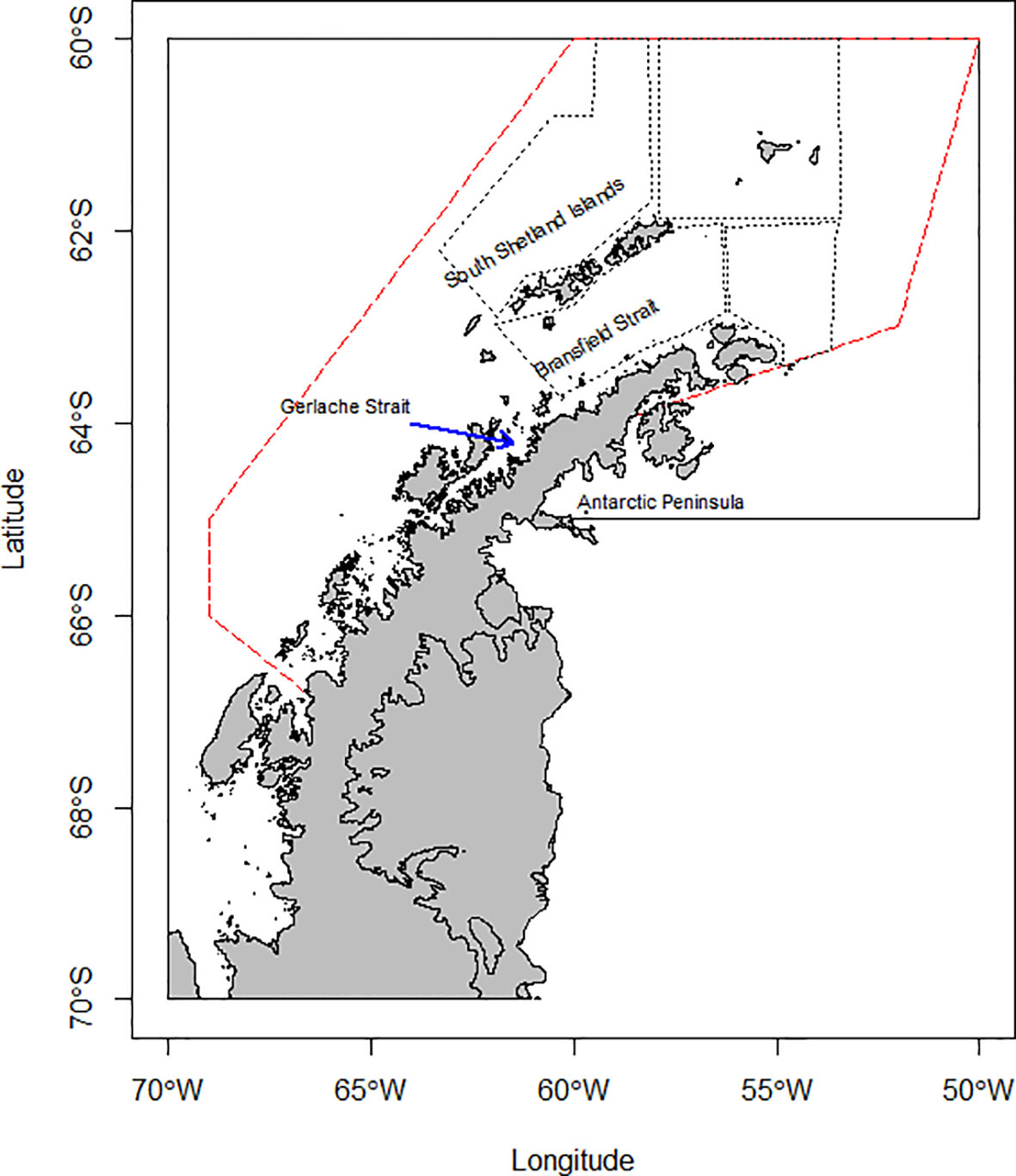
Figure 1 CCAMLR Subarea 48.1 (continuous line) with the operational footprint of the krill fishery from 1979/80 to 2017/18 (red dashed line; from Trathan et al., 2018) and the strata surveyed for krill by U.S. Antarctic Marine Living Resources program (black dotted line, Reiss et al., 2008).

Temporal scale

The risk assessment framework has the ability to operate at any temporal scale if relevant data are available. Data for most species are limited to specific periods during their annual cycle, and data for much of the rest of the year are sparse or non-existent. The temporal scale in our analyses is at the seasonal scale, considering summer (October to March) and winter (April to September) separately. We recognise that this does not fully reflect the intra-annual variation in ecosystem dynamics and the implications of this are discussed below. Further, we highlight that the temporal alignment of the summer breeding season for any given species rarely coincides with the temporal alignment of other species. This means that the full temporal complexity of ecosystem risks is unlikely to be captured in its entirety.

Predator krill requirements

Summer

Raster layers describing the at-sea distribution and density of flying seabirds (Figure S1) were created as described in (Warwick-Evans et al., 2021). Briefly, hurdle models were used to model the density and distribution of 11 species of procellariform seabirds using nine years of data obtained from at-sea surveys conducted between January and March by the U.S. Antarctic Marine Living Resources (AMLR) Program (Figure 1). These distribution rasters were used to estimate spatially explicit krill consumption by each species, by combining estimated energy requirements calculated from Field Metabolic Rates (Shaffer, 2011) with estimates of the proportion of krill in the diet of each species (Croxall et al., 1985) and the energy density of krill (Clarke, 1980).

Warwick-Evans et al. (2022b) describe the approach to estimate krill consumption by three species of Pygoscelis penguins, fin whales Balaenoptera physalus, humpback whales Megaptera novaeangliae and Antarctic fur seals Arctocephalus gazella (Figure S1). For each cetacean species, sightings data were collected from ship surveys conducted between January and March 2013 - 2020 by the Brazilian Antarctic Program (PROANTAR). For fur seals, sightings data were collected between January and March 2003 – 2011 by the U.S. AMLR. Sightings data were used to create species distribution models to predict the distribution and density of each species (independently) in the study area. These were multiplied by consumption estimates for individual cetacean species by Reilly et al. (2004), and fur seals by (Boyd, 2002) to estimate the spatially explicit consumption of krill by humpback and fin whales and fur seals within the study area.

For penguins, generalised additive models were used to predict the distribution of breeding adult chinstrap Pygoscelis antarcticus, gentoo Pygoscelis papua and Adélie Pygoscelis adeliae penguins within the study area, using tracking data collected during the chick-rearing period on the Antarctic Peninsula and South Shetland Islands. Population estimates from the Mapping Application for Penguin Populations and Projected Dynamics data portal (MAPPPD, Humphries et al., 2017) were used to predict the distribution of all populations within the study area. Energy requirements from Croll and Tershy (1998) were combined with estimates of the proportion of prey in the diet of each species (Hinke et al., 2007) to estimate spatially explicit krill consumption by Pygoscelis penguins. See also Trathan et al. (2018; Trathan et al., 2022).

Raster layers for the summer distributions and abundances of pack-ice seals and finfish were created using data from Hill et al. (2007) and Forcada et al. (2012), and converted into estimates of consumption for these species at the Small Scale Management Unit (SSMU, Hewitt et al., 2004) scale by Constable (2016). These data provide the best available estimates for these species (Figure S2).

Winter

Data reflecting the distribution and abundance of krill predators in winter are sparse. Nevertheless, to develop the winter data layers for the risk assessment, we necessarily required estimates of abundance for key species.

The surveys to estimate the abundance and distribution of humpback and fin whales were carried out between January and March. We assume that humpback whales forage in the study area for approximately 120 days per year (Lockyer, 1981); however, this period continues beyond March (when our summer period ends) as aggregations of humpback whales have been observed into June and July (e.g. Nowacek et al., 2011; Weinstein and Friedlaender, 2017). Fin whales have been recorded in the area between February and June, averaging 51 days per year (Širović et al., 2004). However, given that no abundance estimates exist for these species during winter, for the purpose of this risk assessment we have assumed that all krill consumption by whales occurs during summer, when the surveys were undertaken. We recognise the limitation of adopting this approach, which we consider further in the discussion.

Surveys for flying seabirds are also undertaken only in summer and there is little information on the distribution or abundance of flying seabirds in the study area during winter. In summer, flying seabirds account for approximately 2% of the overall krill consumption in the area (Warwick-Evans et al., 2022b), consequently for the purpose of this risk assessment we have assumed that there is no krill consumption by flying seabirds in the study area during winter, something again that we consider in the discussion.

To estimate the winter distribution of adult gentoo penguins the locations and population estimates of gentoo penguins breeding in the study area were obtained from MAPPPD (Humphries et al., 2017). Gentoo penguins remain coastal during the winter months but are not constrained to remain near breeding colonies (Tanton et al., 2004). As such, we have assumed that an even distribution of individuals occurs within 30 km of the coastline of the South Shetland Islands and west Antarctic Peninsula. The distribution was limited to include only areas north of 65.5°S given the most southerly gentoo colony is located at 65.26°S (Figure S3).

Over winter, 62% of adult chinstrap penguins tracked from three colonies on the South Shetland Islands remained local (within 500 km of the colony) (Hinke et al., 2019). The average maximum distance travelled by “local” individuals across these three colonies was 189 km. Therefore, to approximate the winter distribution of chinstrap penguins we have assumed that 62% of all chinstrap penguins that breed in the study area (Humphries et al., 2017) remain within 189 km of the coastline of the South Shetland Islands and western Antarctic Peninsula and are distributed evenly within this area. Although no colonies exist in the south of the study area, Hinke et al. (2019) showed chinstrap penguins continued to visit these southerly areas during winter, and as such, the distribution of chinstrap penguins was not constrained to the northern section of the study area (Figure S3).

Winter tracking of Adélie penguins breeding at Admiralty Bay on the South Shetland Islands have been carried out using geolocator (GLS) devices that use the timing of dawn and dusk to estimate position (Hinke et al., 2015). These location data were therefore used to estimate the winter distribution of Adélie penguins in the study area. Positions north of 55°S were removed from the data as these are likely to represent locations during the equinox when GLS positions are challenging to interpret (Ekstrom, 2004; Hinke et al., 2015). The remaining positions (including those outside of our study area) were gridded into 30 km by 30 km grid cells to create a continuous grid reflecting the sum of the number of GLS positions recorded in each cell (finer resolution grids showed a very patchy distribution which did not smooth across GLS locations). The relative importance of each grid cell was calculated by dividing the value of each cell by the total of all cells. Estimates of the number of breeding adults from all colonies in the study area were downloaded from MAPPPD. Although penguins from just one colony were tracked, it is likely that Adélie penguins from colonies across the northern Antarctic Peninsula and South Shetland Islands follow a similar distribution. Adélie penguins breeding in colonies towards the south of the study area (9% of all Adélie penguins breeding in the study area) are likely to move westerly from the Peninsula following the expanding sea-ice edge and follow an alternative distribution pattern (see Erdmann et al., 2011). Consequently, individuals breeding at these southerly colonies have been excluded from this analysis. The total krill consumption by all Adélie penguins in the north of the study area were distributed across the raster according to the importance of each cell to create spatially explicit krill consumption estimates for Adélie penguins.

No estimates of the energetic requirements of Adélie or chinstrap penguins outside of the breeding season exist, although Hinke and Trivelpiece (2011) have calculated this for gentoo penguins. Consequently, for all species of Pygoscelis penguins the summer estimate of daily krill consumption per individual have been combined with species-specific distribution rasters to estimate the spatially explicit krill consumption by Pygoscelis penguins during winter.

Data layers for the winter distribution and abundance of fur seals, pack-ice seals and fish were created using data from Hill et al. (2007) and Forcada et al. (2012), as used by Constable (2016). These data are at the scale of SSMUs and provide the best available estimates for these species.

Krill distribution

The distribution of krill across the study area was estimated using generalised additive mixed models (GAMMs) as described by Warwick-Evans et al. (2022a). Analyses were conducted independently for summer and winter. Briefly, acoustic sampling methods were applied to estimate the density of krill along transects in the Bransfield Strait and north of the South Shetland Islands and Elephant Island annually in January-March (summer) between 1999 and 2011 and in August-September (winter) between 2012 and 2016 by the U.S. AMLR Program (Figure 1). GAMMs with year as a random effect were used to model the relationship between observed krill density and environmental variables, and to predict the distribution and density of krill across the study area. The krill biomass estimates for winter were also adjusted as described in the ‘modified risk assessment’ section below.

The proportion of juvenile krill was calculated using data from Perry et al. (2019) who used the KRILLBASE database (Atkinson et al., 2017) to determine distribution maps of all krill life stages, using data from 1970-2016. We summed the distribution of adults and juveniles and calculated the proportion of juveniles over two temporal scales, early (October to December) and late (January to May). Krill spawning occurs from December to March (Meyer et al., 2020), and thus we have assumed the early distribution will be similar to the winter distribution, and late season approximately represents the summer distribution.

Fishery desirability

The desirability of an area to the krill fishery was calculated at the scale of 10 km x 10 km following methods by Constable (2016). This analysis focussed on the spatial extent of fishery operations between 2013 and 2018 (Trathan et al., 2018; Trathan et al., 2022). This was prior to the implementation of the Association of Responsible Krill harvesting companies (ARK) voluntary buffer zones (Godø and Trathan, 2022), after which point the distribution of the fishery was restricted as a result of seasonal temporary voluntary restrictions imposed by the krill fishing industry (this strategy was evaluated in a separate scenario). Fisheries catch data during summer and winter were analysed separately. The importance of each 10 km x 10 km cell to the fishery was calculated by dividing the annual seasonal catch from each cell by the annual seasonal total catch within the study area and taking the mean value across all years.

Scenarios

Previously, CCAMLR (WG-EMM-02) identified Small Scale Management Units (SSMUs) as potential units for subdividing the krill catch (SC-CCAMLR-XXI, 2002; Hewitt et al., 2004). However, catch limits at this scale have yet to be implemented. Further, the SSMUs were identified almost two decades ago at a time when the fishery in Subarea 48.1 largely operated to the north of the South Shetland Islands (CCAMLR, 2018a) and before knowledge was available about cetacean recovery in the region (Branch, 2011; Leaper and Miller, 2011; Jackson et al., 2015). As such, SSMUs may not represent the optimal units of management to spread the risk associated with the krill fishery. Nevertheless, we evaluate the SSMUs within the risk assessment, together with a number of other scenarios.

We evaluated the variation in regional risk and in the spatio-temporal distribution of the catch limit associated with managing the fishery according to a variety of management units. We have evaluated 36 scenarios to divide Subarea 48.1 into smaller management units using:

a. A buffer from land (variations ranging from 20 to 50 km, also including internal subdivisions within the buffers). In this context the term buffer is a way to delineate management units adjacent to the coast and islands and does not mean no-take zones (unless specified);

b. Bathymetric contours (variations at 500 m, 750 m, 1000 m, and simplified variations);

c. The top 25% and 50% of predator consumption areas;

d. Regular grid cells (variations ranging from 50 to 200 km);

e. An approximately north-south division across the study region (termed vertical split), an approximately east-west division (termed horizontal split), an approximately north-south division combined with an approximately east-west division (termed 4-way split);

f. The total area used by the fishery from 1980 to 2018, the total area used by the fishery 2013 to 2018 during summer and during winter;

g. The current SSMUs ( (SC-CCAMLR-XXI, 2002) Hewitt et al., 2004);

h. The ARK voluntary buffer zones (Godø and Trathan, 2022; Trathan et al., 2022);

i. The component areas that comprise the proposal for a marine protected area in Domain 1 (D1MPA (see Pew, 2020)); and

j. The strata from the U.S. AMLR acoustic surveys for krill (with variations).

For the scenarios using the ARK voluntary buffer zones and the D1MPA, we set the catch value in each of the no-take zones to zero (summer only for the ARK voluntary buffers). We also note that the D1MPA was proposed for various protection, conservation and management reasons and not solely as a means to manage the krill fishery (Argentina and Chile, 2019). Thus, the risks associated with this scenario should not be considered to reflect upon the intended purpose of this MPA proposal.

The risk assessment assumes that catch is spread evenly within each management unit. However, we know that this is not the case (Trathan et al., 2018; Trathan et al., 2022), and that the fishery is likely to concentrate within preferred areas within management units. This means that the relative risk estimated using the risk assessment framework will not accurately reflect the risk that these management scenarios would represent in practice. As such, for some of these scenarios we have also split the candidate management zones into smaller zones to ensure that the risk assessment measures the risk of the fishery concentrating within candidate management areas (i.e. 50 km buffer from land – see a. above).

Applying the risk assessment framework

We follow the approach of Constable (2016) and Constable et al. (In Review), without variation, in implementing the risk assessment, as this approach has been endorsed by the Commission (CCAMLR, 2019, paragraph 5.17). As CCAMLR becomes more familiar with the approach, fine tuning of the inputs and their equations are plausible.

Risk

Data layers describing krill consumption (tonnes day^-1 km^-2) by flying seabirds, penguins and fur seals were summed to create seasonal layers (summer and winter) of krill consumption by central place foragers (CPF). Data layers describing the krill consumption (tonnes day^-1 km^-2) by whales, fish and pack-ice seals were summed to create seasonal layers describing krill consumption for ideal-free or pelagic (PEL) species. Total seasonal krill demand by CPF and PEL predators was calculated by dividing the daily estimates of krill consumption within each candidate management unit by the area of the candidate management unit (km²) and scaling this to provide seasonal estimates by multiplying these values by 182 (i.e., to correspond to the nominal durations of summer or winter). Seasonal predation pressure was calculated for each candidate management unit by dividing the krill demand by the krill density. Predation pressure (X) was scaled to range from 0 – 1 using a logistic function to assist with scaling the component factors, f, between 0 and 1 (Equations 1.1 and 1.2, methods described by Constable (2016), (Constable et al, 2002. in review)).

$\begin{array}{ll}1\left(X\right)=\frac{1}{{\left(1+e^{-h(X-X50)}\right)}^{\frac{1}{v}}}& \text{Equation 1.1}\end{array}$

$\begin{array}{ll}f=Y0+Yr\left[\frac{1(X)-1(X0)}{1(X1)-1(X0)}\right]& \text{Equation 1.2}\end{array}$

where h is the steepness parameter, X50 is the value for x for which the function gives a value of 0.5, and v is a shape parameter. X0 is the X value for which the function value would be offset to 0. X1 is the value for X for which the function is scaled to 1. Y0 is the minimum value where Y0 >= 0. Yr is the range, where (Y0 + Yr) <= 1. Values for the parameters used to scale the predation pressure were h=3, v=3, X50 = 0.5, X0 = 0, X1 = 4, Y0 = 0, Y1 = 1. Also see Kelly et al. (2018) and (Constable et al, 2002. in review) for more details on the logistic scaling function.

Indices of risk (r) were calculated for summer and winter using Equation 2 where CPF is the scaled predation pressure of central place foragers, PEL is the scaled predation pressure of pelagic predators, and JUV is the proportion of juvenile krill.

$\begin{array}{ll}r=1-\left(\left(1-JUV\right)*\left(1-CPF\right)*\left(1-PEL\right)\right)& \text{Equation 2}\end{array}$

Desirability

Seasonal desirability by the fishery was scaled to range from 0 to 1 using Equations 1.1 and 1.2. Values for the parameters used to scale the fishery desirability were h=60, v=1, X50 = 0.08, X0 = 0, X1 = 1, Y0 = 0, Y1 = 1 following Constable (2016).

Assessment of alpha

Alpha (α, the proportion of catch to be taken from each area) was calculated using Equation 3, where r is risk, c is fisheries desirability, Z is the proportion of annual catch, K = krill density (tonnes km^-2), A is area (km²), _a is local area (i.e. management unit), _p is a specific period (i.e. summer or winter), _a’is across all areas and _p’ is during all periods. We set the proportion of the annual catch taken during summer = 0.38 and winter = 0.62, which reflects the fisheries operations prior to establishment of ARK voluntary buffer zones (2013-2018). These values could be changed in future implementations to reflect any changes in fisheries operations. However, one of the output results from the assessment of risk, is altered proportion of catch limits assigned to summer and winter.

$\begin{array}{ll}{a}_{a,p}=\frac{\left((1-r_{a,p}\right)*c_{a,p}*z_{a,p}*K_{a,p}*A_{a,p})}{{\displaystyle {\sum }_{a^{\text{'}},p^{\text{'}}}\left((1-r_{a^{\text{'}},p^{\text{'}}}\right)*c_{a^{\text{'}},p^{\text{'}}}*z_{a^{\text{'}},p^{\text{'}}}*K_{a^{\text{'}},p^{\text{'}}}*A_{a^{\text{'}},p^{\text{'}}})}}& \text{Equation 3}\end{array}$

Baseline risk

The baseline risk provides a means of identifying which management units may result in the overall lowest regional risk to predators and krill when the desirability of the fishery is not taken into account. This can be used to identify the proportion of the catch to be taken from each management unit in each season to spread the risk and not disproportionately affect some areas more than others. The baseline risk is calculated by setting the fisheries desirability to 1 for all locations and all periods. The baseline regional risk $\stackrel{⌢}{R}$ is calculated using Equation 4 where â_a,p is the baseline alpha for the scenario where c = 1 (i.e., identity multiplier as no information on desirability is conveyed in this risk estimator).

$\begin{array}{ll}\widehat{R}= {{\sum }^{}}_{a,p}{r}_{a,p}{\widehat{a}}_{a,p}& \text{Equation 4}\end{array}$

Desirability risk

The desirability by the fishery can be incorporated into Equation 3 by setting the value of c to the scaled value for the seasonal desirability by the fishery. From this we can calculate new values for alpha for each management unit and a new regional risk R_d. This provides a means of identifying which management units may result in the lowest regional risk to predators and krill when the desirability of the fishery is taken into account. If R_d > $\stackrel{⌢}{R}$, the regional risk of localised effects of the fishing has increased above the baseline. The ideal scenario would be to identify management units with a low baseline risk, which does not increase when fisheries desirability is taken into account. If the desirability scenario increases the risk, then it is possible to introduce offsets to close high risk areas or reduce the catch limit in order to not exceed the baseline regional risk (Constable et al, 2002. In review).

Modified risk assessment framework

Adjusting winter krill biomass estimates

The density and distribution of krill vary seasonally at the west Antarctic Peninsula (Lascara et al., 1999, Reiss et al., 2017), with important consequences for both predators and the commercial fishery. Similar intra-annual patterns of density have been established elsewhere (Saunders et al., 2007, Reid et al., 2010), suggesting intra-annual variation in krill probably reflects some key ecological property of krill life-history. Plausibly, biomass is likely to increase during spring and summer, as a result of spawning and somatic growth, whilst continued mortality and transport in ocean currents away from a region may result in decreased biomass during winter.

Our estimates of krill biomass during winter were considerably lower than those for summer which were based on long-term averages. Model validation suggests that the winter models are robust in their predictions of krill distribution within the study area. This is consistent with previous studies; for example, at the west Antarctic Peninsula, Lascara et al. (1999) reported that spatially averaged estimates of krill biomass were an order of magnitude higher during spring (32 gm^-2) and summer (95 gm^-2), than during autumn (12 gm^-2) and winter (8 gm^-2). Nevertheless, the winter krill surveys were conducted during 4 years where krill biomass was lower than average (WG-EMM-2021/05 R1), so the winter estimates of krill biomass may be lower than the long-term average.

During WG-EMM in 2021, some scientists were concerned that these low estimates of biomass in winter may not properly reflect the long-term ecological situation in the west Antarctic Peninsula and suggested that the winter estimates of biomass need to be adjusted. As such we have evaluated each management scenario after updating the winter krill distribution model to have the same total biomass as for summer, whilst maintaining the spatial variation in the distribution between summer and winter. This was achieved by dividing the value of each cell in the winter raster by the sum of all cells in the winter raster to obtain the importance of each cell (summing to 1), then multiplying this by the total biomass estimated from the summer model (which is a long-term average).

We have compared the outcomes using both the original and adjusted estimates for winter krill biomass, to better understand how the uncertainty in this layer could lead to different outcomes of the risk assessments. Determining a more realistic biomass estimate for krill during the winter is now urgent, if CCAMLR is to properly assess risks to the ecosystem.

Accounting for uneven spatial spread of catch

One of the key assumptions of the risk assessment is that the catch within each management unit is harvested evenly from across that management unit. In Subarea 48.1, historical fishing patterns (Trathan et al., 2018; Trathan et al., 2022) show that the fishery actually concentrates at a finer scale (Appendix 2).

Thus, to account for the concentration of the fishery within candidate management units and better characterise the relationship of the fishery with the risks in the management units, we have implemented the risk assessment at a scale more closely aligned with the scale at which we believe the fishery operates. We have used a selection of the lowest risk scenarios and scenarios where management would be plausible (i.e. without very large numbers of management units). As such, within those management units in which the fishery operated (2013 - 2018, summer and winter), the risk assessment was run assuming that all catch would be taken within the footprint of where the fishery actually operated, rather than spread evenly across each management unit. For management units where the fishery did not operate, we have assumed that there would be an even spread of catch within each management unit. Though this assumption is unlikely, we have no prior information about where the fishery would operate in these areas. Figure 2 provides an example to illustrate how we have implemented this. This implementation used the adjusted winter krill layer as described above.

FIGURE 2

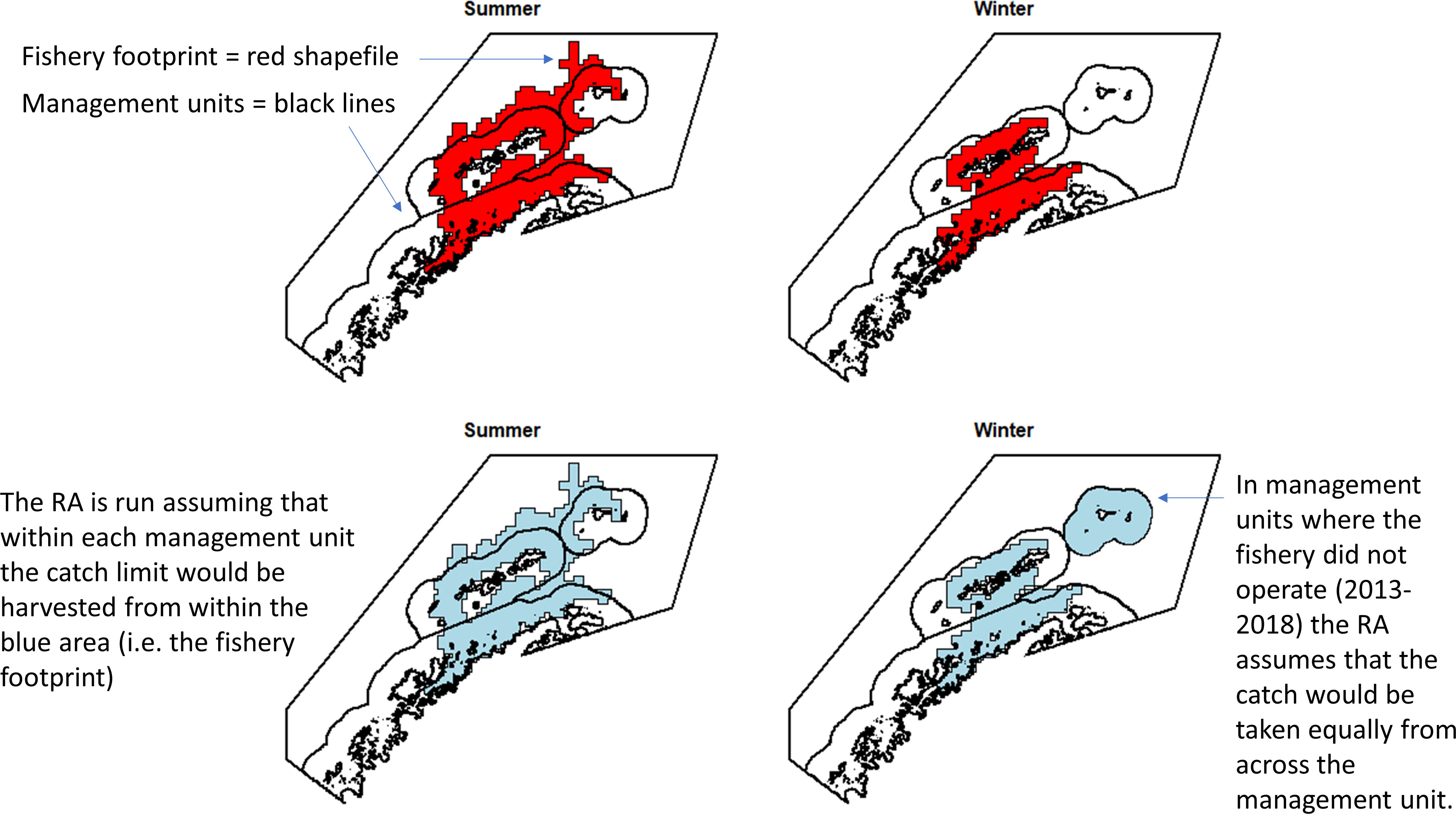
Figure 2 Example, using the 50 km buffer scenario, of how the risk assessment (RA) was run at a scale similar to that at which the fishery operates. This assumes the catch limit would not be taken equally across a management unit but would be concentrated according to previous behaviour of the fishery. This means that the risk is actually calculated from the blue areas, not the management unit areas.

Results

Estimated daily consumption of krill across the study area during summer was highly variable between groups. Fish were estimated to have consumed 76% of the summer daily krill consumption in the area, followed by fin whales (11%), humpback whales (6%), chinstrap penguins (4%), Adélie penguins (3%), flying seabirds (2%), pack-ice seals (2%), gentoo penguins (0.2%) and fur seals (0.1%). Fish also consumed 76% of all krill consumed during winter, followed by pack-ice seals (8%), chinstrap penguins (7%), Adélie penguins (5%), gentoo penguins (2%) and fur seals (1%).

Detailed results of the regional risk and the total proportion of the catch that could be taken from each management unit during summer and winter, for both baseline and desirability scenarios are presented in Appendix 4. For all scenarios, a higher proportion of the catch was assigned by the risk assessment method to the summer period than to winter. In most cases, including the desirability for the krill fishery caused desirability regional risk to exceed baseline regional risk. For the majority of scenarios the baseline scenario assigned the majority of the catch limit to the outer management units (away from the coast), and the desirability scenario assigned the majority of catch to the Bransfield and Gerlache Straits.

The baseline regional risk varied from 0.62 to 0.84 (Table 1; Appendix 3) and was lowest when the 50 km grid cells were used as candidate management units (Figure 3). As the grid cells incrementally increased in size, the risk increased. In general, smaller scale management units had lower risk, as it is more feasible to capture the risk and assign catch to lower risk areas in these scenarios. The desirability regional risk varied from 0.68 to 0.81 (Table 1; Appendix 3) and was lowest when the 500 m bathymetry contour was used as candidate management units (Figure 4). Using a slightly simplified version (where just the three main shelf areas were included rather than all of the small areas where bathymetry < 500 m, see Appendix 4) showed the same level of risk as when the detailed isobaths were used to delineate candidate management units (Appendix 4). The scenarios using existing SSMUs as candidate management units also had relatively low risk. The scenarios using different buffer distances from the coast showed higher risks. As the distance from shore increased, the baseline risk decreased whereas the desirability risk increased. The scenarios using isopleths of predator krill consumption as candidate management units also showed higher risks, though the management units defined by these isopleths were small and patchily distributed. The scenarios using the existing fisheries distribution to delineate candidate management units resulted in some of the highest risk levels, with the highest risk level when the area used by the fishery from 2013-2018 during winter was used to define the management units.

TABLE 1

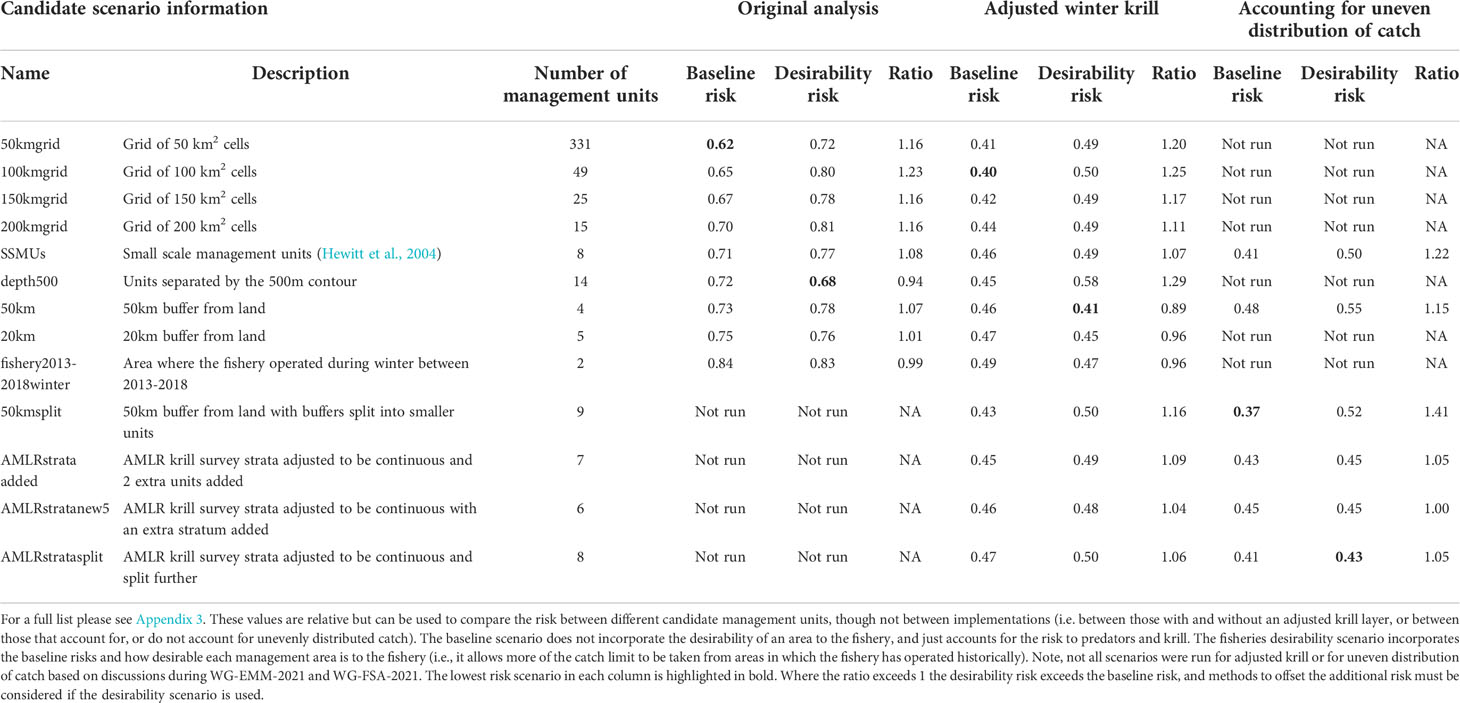
Table 1 A selection of scenarios detailing the relative risk from each candidate management scenario assuming the proportion of catch is taken from each management unit as detailed in Appendices 2–4.

FIGURE 3

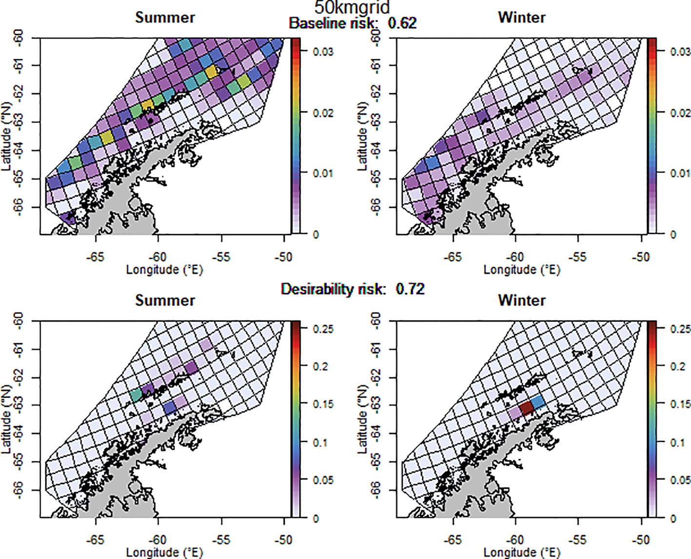
Figure 3 The proportion of the annual krill catch limit that could be taken from each management unit (50 km x 50 km grid cell) during summer and winter if the grid cell management units are used, when the initial analysis for the risk assessment was implemented (i.e. unadjusted layer for winter krill and assuming even catch distribution within management units). Values sum to 1 across all management units and for both seasons for each of the baseline (upper panel) and desirability (lower panel) scenarios.

FIGURE 4

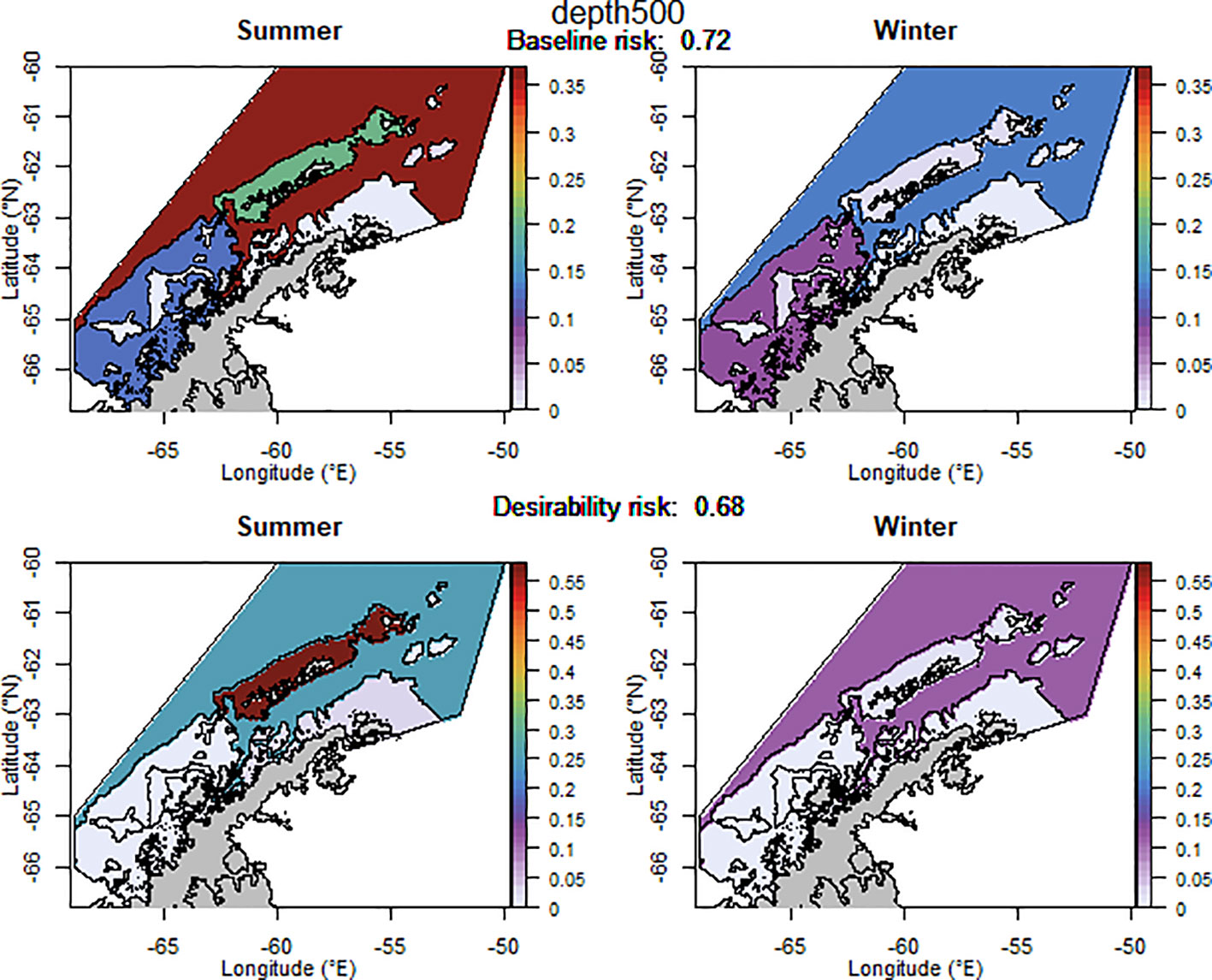
Figure 4 The proportion of the annual krill catch limit that could be taken from each management unit (delineated using a simplified version of the 500 m isobath) during summer and winter when the initial analysis for the risk assessment was implemented (i.e. unadjusted layer for winter krill and assuming even catch distribution within management units). Values sum to 1 across all management units and both seasons for each of the baseline (upper panel) and desirability (lower panel) scenarios.

Modified risk assessment framework

Adjusting winter krill biomass estimates

For all scenarios where the krill biomass was adjusted to be equal to the summer krill biomass (based on the recommendation of WG-EMM-2021, see above), a higher proportion of the catch was assigned to the winter period than to summer. In most cases, including the desirability to the krill fishery caused very little catch to be assigned to summer, and desirability regional risk to exceed baseline regional risk. For the majority of scenarios the baseline scenario assigned the majority of the catch limit to the outer management units, and the desirability scenario assigned the majority of catch to the Bransfield and Gerlache Straits.

The baseline regional risk varied from 0.40 to 0.49 (these values are not comparable with those mentioned above as different krill data layers were used in the analyses, Table 1; Appendix 5) and was lowest when the 100 km grid cells were used as candidate management units. When the desirability of the fishery was also taken into account the regional risk ranged from 0.41 to 0.62 and the 50 km buffer from land had the lowest risk (Figure 5). The scenarios based on the U.S. AMLR krill survey strata also had relatively low risk. The U.S. AMLR scenario with 2 additional management units had a lower baseline risk, and the desirability risk was lowest in the scenario with one extra management unit.

FIGURE 5

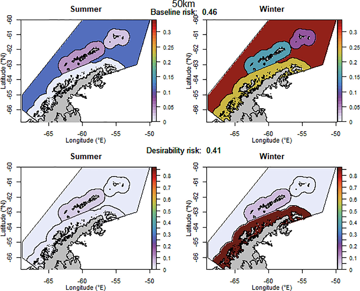
Figure 5 The proportion of the annual krill catch limit that could be taken from each management unit (delineated using the 50 km buffer from land) during summer and winter when the risk assessment was implemented after the winter krill layer was adjusted. Values sum to 1 across all management units and both seasons for each of the baseline (upper panel) and desirability (lower panel) scenarios.

The scenarios using bathymetry to delineate candidate management units also had relatively low baseline regional risk, lowest when using a 500 m isobath. However, in the desirability scenarios, using bathymetry resulted in some of the highest levels of risk (Table 1). The scenarios using existing SSMUs as candidate management units also had relatively low risk.

Accounting for uneven spatial spread of catch

For selected scenarios, using the adjusted krill biomass (winter biomass equal to the summer biomass; based on the recommendation of WG-EMM-2021, see above), the baseline regional risk varied from 0.37 to 0.58 (Table 1; Appendix 6). The lowest risk baseline scenarios were those where candidate management units were delineated using the 50km buffer split into smaller management units (Figure 6), followed by the original SSMUs and the U.S. AMLR survey strata, split further into additional management units (Figure 7). We did not evaluate some of the lower risk scenarios from previous implementations (i.e regular grid cells), given the complex requirements to manage at these small scales, with numerous or patchy management units. The desirability regional risk varied from 0.43 to 0.58 (Table 1; Appendix 6). The lowest risk desirability scenarios were those where candidate management units were delineated using the U.S. AMLR survey strata, split further into additional management units (Figure 7). The next lowest risk scenarios were using the U.S. AMLR strata with additional management units added (Figure 8).

FIGURE 6

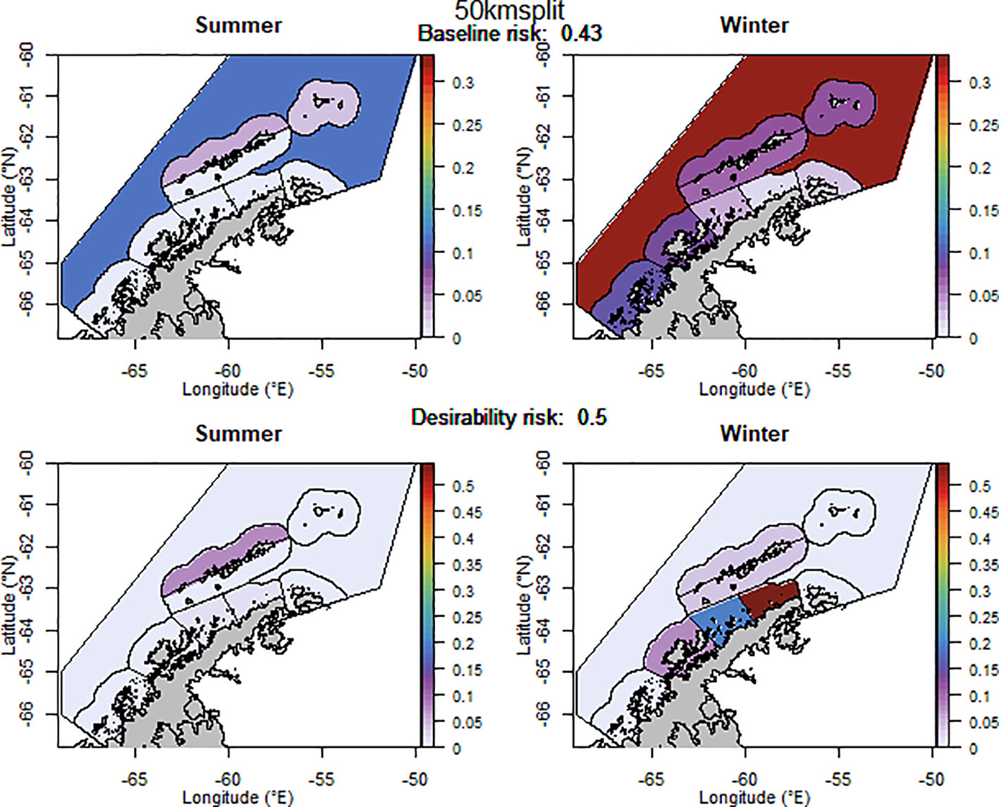
Figure 6 The proportion of the annual krill catch limit that could be taken from each management unit (delineated using the 50 km buffer from land divided into smaller management units) during summer and winter when the risk assessment was implemented after the winter krill layer was adjusted. Values sum to 1 across all management units and for both seasons for each of the baseline (upper panel) and desirability (lower panel) scenarios.

FIGURE 7

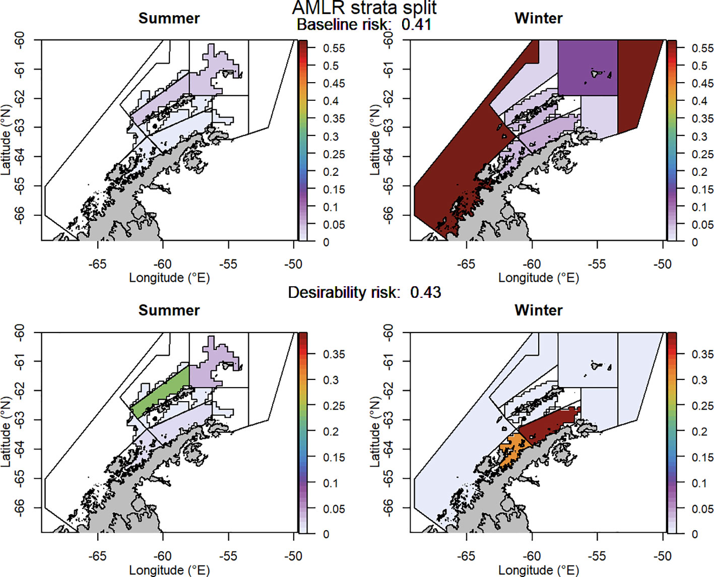
Figure 7 The proportion of the annual krill catch limit that could be taken from each management unit (delineated using the US-AMLR survey strata divided into smaller management units) during summer and winter when the risk assessment was implemented after the winter krill layer was adjusted and assuming catch is not evenly distributed within management units. Values sum to 1 across all management units and for both seasons for each of the baseline (upper panel) and desirability (lower panel) scenarios.

FIGURE 8

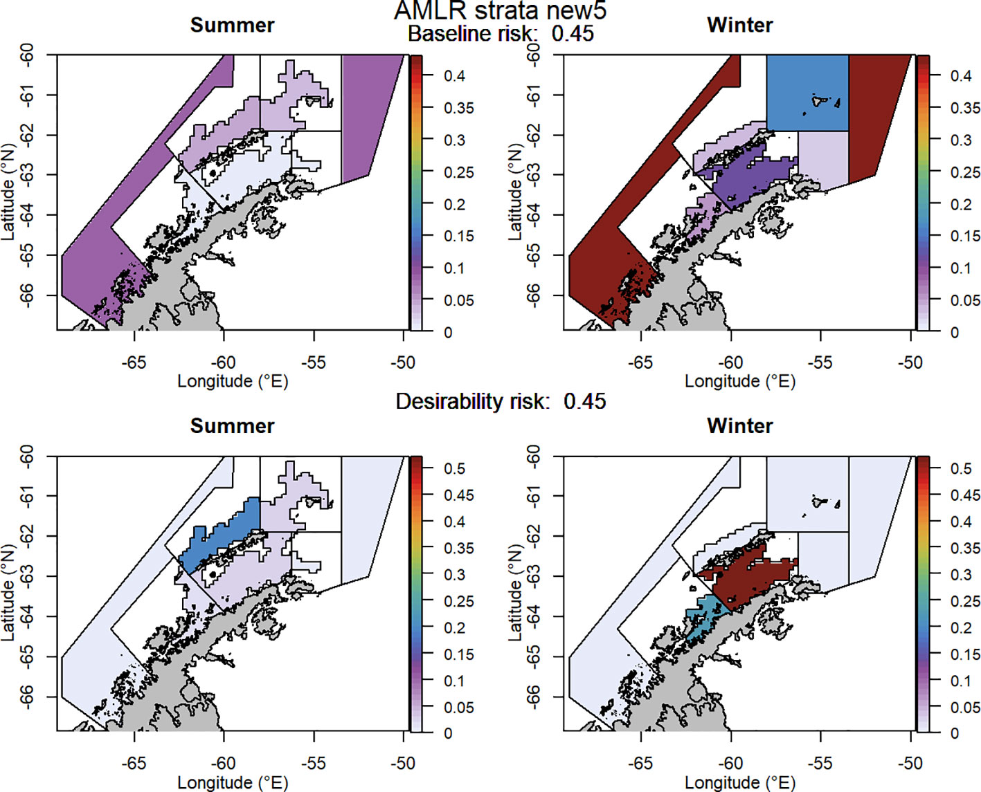
Figure 8 The proportion of the annual krill catch limit that could be taken from each management unit (delineated using the US-AMLR survey strata with an added management unit) during summer and winter when the risk assessment was implemented after the winter krill layer was adjusted and assuming catch is not evenly distributed within management units. Values sum to 1 across all management units and for both seasons for each of the baseline (upper panel) and desirability (lower panel) scenarios.

Discussion

We have applied the risk assessment framework developed by Constable (2016) and Constable et al, 2002. (in Review) to Subarea 48.1 in order to evaluate alternative management units which can be used to spatially and temporally distribute the catch limit of the krill fishery, given our access to the best available science. We have evaluated 36 scenarios and found that using a regular grid with small grid cells leads to the least risk. However, these scenarios, with large numbers of management units would probably be highly complex to manage, particularly given the complexities of advance notification to the fishery of dates when management areas will be closed. Also, fine-scale delineation of management units may not be appropriate due to uncertainty in the data layers. In contrast, the scenarios using the scale and location at which the fishery currently operates resulted in some of the highest risks of all scenarios evaluated.

Our results suggest that in order to minimise risk, spatial management needs to occur at scales smaller than the Subarea scale, and that managing at small scales at least in those areas where the fishery operates is important for maintaining CCAMLR’s precautionary approach to management. We discuss our findings in two parts. First, how the fishery might be structured spatially and temporally in Subarea 48.1. Second, what the next steps will be to refine this process as CCAMLR moves forward with developing a sustainable fishery.

Choosing the appropriate framework for krill fishery management

Baseline or desirability risk

During the early development of the risk assessment approach the concept of desirability was introduced because baseline scenarios tended to assign the majority of the catch limit to the outer management units (remote from the coast), to locations where the fishing industry had previously rarely operated. As such, and given the diversity of views about protection, conservation and fishing held by different CCAMLR Members (see Godø and Trathan, 2022), use of management units that forced the fishery into the outer units would probably remain challenging. However, desirability helps with this, particularly if and when catch limits increase. If evidence shows catches can increase, at some point desirable management units may need to receive capped catch allocations in order to ensure overall risk does not increase beyond the baseline risk. Thus, the inclusion of desirability remains a key issue, and as such we focus our discussion on those scenarios that take into account desirability.

Original or adjusted winter krill biomass

It is likely that our models underestimate krill biomass during winter as they were based on four years of data when biomass was lower than average. However, krill biomass during winter should plausibly be lower than during summer (e.g. Lascara et al., 1999). By using the upscaled estimates of winter krill biomass, more of the catch limit is assigned to winter than summer, the opposite of the original implementation. By increasing krill biomass, predation pressure is reduced, resulting in lower estimates of risk during the winter period, and thus allowing increased catch limits during this time. As such, the seasonal estimates of krill biomass are highly influential to the temporal assignment of krill catch limits. Nevertheless, because upscaling of winter biomass estimates was requested by WG-EMM, we focus our discussion using results from these adjusted analyses.

Even or uneven spatial spread of catch

In implementing the risk assessment at scales that reflect the current operation of the krill fishery (e.g. Figure 2), we account for the assumption that all catches within a given management unit are evenly distributed. We do this by restricting catch within each management zone to reflect the current operation of the fishery providing a more realistic estimate of risk, even though we could not fully implement this for management units where the krill fishery has not operated previously, given the absence of knowledge about preferred fishery distributions. Accounting for the concentration of the fishery within candidate management units does offer a better representation of risk. As such, we focus the rest of the discussion on the scenarios where we attempt to account for risk in this way.

Determining an appropriate spatial and temporal management structure for the krill fishery

Temporal distribution of catch

A higher proportion of catch was assigned to winter than to summer in all scenarios (using the adjusted winter krill biomass estimates), with <30% assigned to summer in most cases. This is not surprising given the presence of large numbers of breeding penguins and cetaceans that depend on krill during the summer. Additionally, consumption by finfish, which make up a large proportion of overall krill consumption is very much reduced in winter (see Appendix 2). In addition to consumption estimates being lower for winter than for summer, the consumption is more widely distributed as central place foragers are no longer constrained to remain near breeding sites. However, adjusting the winter krill layer so that it matches the biomass of the summer layer effectively reduces risks in winter, which in turn assigns more catch to winter. The degree to which this inadvertently increases risks is unknown.

Spatial distribution of catch

Our original implementation of the risk assessment showed that the management units which had the lowest desirability risk to the ecosystem were those delineated using the 500 m depth contour. However, after adjusting the winter krill layer, the lowest risk scenario occurred when management units were delineated using a 50 km buffer from land. A scenario where the 50 km buffer from land was split further into smaller management units resulted in an increase in risk (in the desirability scenario), emphasising our concerns that the fishery focuses effort within candidate management units and led to our decision to account for an uneven spread of catch.

Of the scenarios tested that assume uneven distribution of catch, the lowest risk management units were those based on the U.S. AMLR survey strata, in particular the scenario where these strata were split into smaller management units (AMLR strata split). In these scenarios, the majority of catch was assigned to the Bransfield and Gerlache Straits during winter, whilst summer catches were assigned north of the South Shetland Islands. Similar scenarios (AMLR strata added and AMLR strata new5) resulted in a similar proportion of catch assigned to the Bransfield and Gerlache Straits. However, in all of these cases, catch concentration occurs in areas preferred by the fishery, meaning these scenarios may not be as suitable for management as they appear. If the purpose of the new management approach is to reduce catch concentration, then limiting the catch to desired areas may be counterproductive.

Scale of management zones and the fishery

We show that risks associated with unconstrained operation within the current areas used by the fishery result in some of the highest risks of all scenarios evaluated. Though risks are relative, and not absolute, this is a major concern, and one already recognised by CCAMLR. Indeed, Kelly et al. (2018) show that the regional risk of the current conservation measures in Subareas 58.4.1 and 58.4.2 exceed baseline risk. This suggests that if catch limits are reached, then predators in these areas could be exposed to disproportionate effects from the fishery.

Extrapolating from analyses based on regular grid cells (50 km, 100 km, 200 km), suggests that larger management areas facilitate concentration of catch, which may deplete local krill populations and increase risk to predators and krill alike (Klein and Watters, 2020). This highlights the need to manage the krill fishery at smaller scales and is consistent with findings by Watters et al. (2020). This has been recognised at the Subarea scale through Conservation Measure 51-07 (CCAMLR, 2016), and now needs to be developed within Subareas (see also Watters et al., 2009). By implementing a small-scale approach to management, CCAMLR would be able to set specific catch limits according to fine scale ecosystem processes, such as consumption by predators, or important areas for krill.

Although it is apparent that managing the fishery at a smaller scale is likely to reduce the risk to the ecosystem, we recognise that this is more challenging from a management perspective than working at larger scales. It is likely that a compromise between risk and simplicity of management will be needed, as has been recognized for nearly three decades (e.g. Watters and Hewitt, 1992). A realistic compromise may be to use finer scale management units in areas of higher risk, and larger scale managements in areas of reduced risk. We are also mindful that managing at very small spatial scales relies on modelled data layers that include spatial (and temporal) error.

In addition to spatial concentration of catch we must consider temporal concentration of catch. If catch limits are reached during winter and remain concentrated in inshore areas such as the Bransfield Strait, there is an increased likelihood that recruiting or spawning females may be disproportionally caught by the fishery (Perry et al., 2019; Meyer et al., 2020). This has the potential to negatively impact both the krill stock and the wider ecosystem. Thus, depletion of winter concentrations of krill by the fishery may lead to impacts on predators in the following spring, when abundant krill supplies may be important to predators in preparation for breeding (Trathan et al., 2021).

A key issue is whether the low-risk scenarios developed from the U.S. AMLR survey strata continue to facilitate concentration of fishing effort at scales that will have ecosystem consequences.

Ecological weighting

There are three main ecological components factored into the assessment of risk; these are the risk to central place foragers, the risk to pelagic species and the risk to juvenile krill. Each are weighted equally in the current implementation (Constable, 2016; Constable et al, 2002. in review).

During summer, central place foragers are constrained to remain near breeding colonies in order to return to land to provision their developing young (Orians and Pearson, 1979). As such, if krill are depleted in areas adjacent to the colony, then the adults must forage further from the colony, potentially resulting in reduced breeding success or reduced adult survival (Ashmole, 1963). For pelagic species this is not the case as they have more flexibility in where they are able to forage and can travel to nearby areas with increased krill density. However, evidence now suggests that individuals of some pelagic species such as humpback whales and pack-ice seals also have preferred feeding grounds (e.g. Burns et al., 2004; Dalla Rosa et al., 2008; Nowacek et al., 2011; Weinstein and Friedlaender, 2017). Some fish species build nests (e.g. Daniels, 1978), but their spatial and temporal dynamics remain largely unknown at scales relevant to the risk assessment.

Information about different life history stages of krill is important, particularly as only certain stages are targeted by the commercial fishery. Risks to the krill stock as a whole could occur if particular stages were to be reduced below any given ecological threshold. As such, risks are likely to reflect different scales of ecosystem operation (Perry et al., 2019; Veytia et al., 2020). Having implemented the risk assessment for Subarea 48.1, coupled with information about commercial net selectivity and the circumpolar distribution of krill, we suggest that CCAMLR might reconsider ecological risks to juvenile krill. For example, it would be useful to determine if krill should be weighted equally to central place foragers and pelagic species. Although it is important to protect krill in early life stages, these early-life stages are widespread, and are not targeted by the fishery. Additionally, it may be important to protect other krill life-history stages such as spawning adults, which may also be impacted by the fishery due to their restricted distribution (Meyer et al., 2020). Weighting the risk to juvenile krill as equal to the risk to central place foragers and pelagic species may therefore be disproportionate.

Model limitations and future work

The approach we have taken to apply the risk assessment, whereby data layers are created for each species and for the fishery, allows us to identify areas of increased risk at fine spatial scales. However, we recognise that some of the predator and krill data layers could be improved, particularly for winter, but also for summer. The estimated proportion of krill consumed by each predator group and the spatial distributions of consumption will influence the outcome of the risk assessment. However, the data we used are the best currently available. Therefore, should CCAMLR continue to use the risk assessment approach in the future, a revision of predator monitoring data will be necessary and this should, at least partially, be designed to parameterise the needs of the risk assessment.

Data gaps

Spatial scale

The available data and modelling approaches we have used for penguins, flying seabirds, Antarctic fur seals, humpback and fin whales and krill allow us to identify important areas at fine spatial scales. However, the best available estimates of the abundance of pack-ice seals, and finfish are at the SSMU scale, which is far broader than the scale of some of the scenarios tested. It is likely that the distribution of species will vary within such broader spatial scales, and plausible that risk to these species may not be adequately captured, especially for winter, when observations are sparse.

In some cases it was necessary to predict habitat-use distributions outside of surveyed areas, and it was not always possible to validate the predictions in these areas. The modelling approaches we used associate observed species distributions with particular environmental characteristics and our predictions assume that these relationships remain consistent across the study area. Although it is probable that the environmental characteristics identified by these models are important drivers of species distributions, there are also likely to be additional factors that influence the distributions of these species (e.g. competition, density dependence, and prior knowledge). Consequently, although our models combine the best available data with robust modelling approaches, it is plausible that they do not fully identify all important areas for some species.

We also note that the U.S. AMLR krill survey area no longer overlaps with much of the area used by the krill fishery, as the fishery has become more concentrated in nearshore shallow waters at depths of <1000 m (Warwick-Evans et al., 2022a). We emphasise that it is important to collect new krill acoustic density data, including in areas representative of those areas where the fishery currently operates, to validate our models. This is also true for all predator species, and without such data, it will remain challenging to parameterise new models and/or to validate the models we have already developed.

Temporal scale

This risk assessment operates at a seasonal scale, with summer and winter considered separately. The distribution of both krill and predators is variable throughout the year (see Appendix 2) and by working at this scale we can begin to capture some of this variation. However, species distributions are likely to be variable within and across these broad temporal scales (e.g. Lascara et al., 1999; Curtice et al., 2015). For example, penguins are most constrained during the chick-rearing period, when these data were collected, with a wider range during the rest of summer (Orians and Pearson, 1979; Warwick-Evans et al., 2018; Warwick-Evans et al., 2019). As such, it is likely that penguins will have a wider distribution than shown in these data layers during some of the summer period. Additionally, the energy requirements of penguins vary considerably throughout the year at finer temporal scales than the seasonal scale at which we are working (Croll and Tershy, 1998). As far as we are aware, the energetic requirements or field metabolic rates of penguins have not been estimated for the winter period, and it was necessary for us to use summer estimates. Energy requirements will be elevated during periods when they are preparing for and recovering from breeding and moult and when provisioning chicks (Croll and Tershy, 1998). As a result, krill consumption will be highly variable throughout the year (e.g. Boyd, 2002; Southwell et al., 2015). Although some of these periods of increased krill consumption will fall during winter it is likely that krill consumption will be considerable during the summer chick provisioning period. As such, it is plausible that we overestimate individual krill consumption by penguins during winter. However, these data layers for penguins consider only breeding adults (and nestlings), and do not account for juvenile or non-breeding individuals. As a result, it is likely that the overall estimates of krill consumption by penguins are conservative (see Boyd, 2002; Emmerson and Southwell, 2017).

We also assumed humpback and fin whales congregate to feed in the study area for approximately 120 days during summer (as per Lockyer, 1981), although more recent estimates suggest that they may inhabit the area into June and July (e.g. Širović et al., 2004; Nowacek et al., 2011; Weinstein and Friedlaender, 2017). As such, this period does not directly align with the October – March definition of summer used in this risk assessment. It was not possible to subdivide these krill-consumption estimates across the seasons defined here as a result of the ongoing uncertainty about the abundance and distribution of whales later in the season. Consequently, by assigning all krill consumption by cetaceans to the summer period we might be underestimating these estimates of predation pressure on krill during the winter months, and potentially overestimating it during summer. If such biases are substantial, more catch would need to be assigned to summer and less to winter.

Ecological data used to assess krill consumption and therefore risk, cannot be neatly partitioned into simple time periods if they are to adequately capture the ecosystem dynamics within the study area. Thus, although it would be meaningful to align the temporal scale of management with the dynamics of the ecosystem, this remains a challenge. In the future, the risk assessment framework may require working at finer temporal scales which highlight periods when risks to predators are greatest, but also recognising restrictions of available data and implementation.

A consequence of this temporal mismatch is the spatial mismatch. Currently, the same management units are used for each season. However, it is plausible that different management unit boundaries may be appropriate in summer and winter.

Additionally, most predator surveys or tracking studies are conducted between January and March, and very little data exists for the winter months. This is important as the autumn and winter period is the time during which the fishery is most active in Subarea 48.1 (Trathan et al., 2022) and thus the ecosystem is potentially most at risk from the fishery. The consequences of these limited data may be variable amongst predator groups. For example, we were not able to estimate the consumption of krill by flying seabirds over winter. However, our estimates of summer krill consumption suggest that they consume approximately 2% of all krill consumed in the study area (Warwick-Evans et al., 2021). It is likely that most flying seabirds will be less abundant during winter as advancing sea-ice may prohibit foraging in the area. Consequently, we believe that excluding flying seabirds from the winter analysis is unlikely to greatly affect the outcome of the risk assessment. However, excluding cetaceans from our winter estimates may have far more impact, due to the quantity of krill they consume.

Similarly, the U.S. AMLR Program has only conducted a limited number of krill surveys during winter, but these allowed us to develop separate layers for krill in summer and winter. However, the estimated krill biomass during winter was considerably lower than estimated summer biomass, and it is plausible that the winter estimate is an underestimate of the long-term winter krill biomass. As a short-term solution on advice from WG-EMM, we have adjusted the winter biomass to match the summer biomass, whilst maintaining the variation in distribution. However, as krill biomass during winter is expected to be lower than during summer (Lascara et al., 1999), we emphasise that this is a short-term solution and that additional krill survey data covering a broader temporal and spatial scale are now urgently needed. This is made more urgent as the krill fishery preferentially operates into winter (Trathan et al., 2022).

Outdated data and missing species

Although we were able to use recent tracking or survey data to estimate the abundance and distribution of some predators, for others these estimates are outdated and may not reflect current population sizes. For example, surveys for pack-ice seals were carried out in 1999, whilst demographic models parameterised with data from the 1990s were used to estimate the abundance of finfish (Hill et al., 2007; Hückstädt et al., 2020). The layer for finfish will have a large impact on the outcome of the risk assessment (~76% of all krill consumed) and thus it is key that these estimates are updated as part of a long-term management strategy. In this study, this will have resulted in lower levels of catch being assigned to areas with higher abundance of finfish. Given that the fish layer currently has a large influence on the model outcome, and we do not include models of their fine-scale distribution we suggest that developing a habitat model using recent trawl data would be useful.

Additionally, population estimates for some penguin colonies are from the 1980s. It is likely that at least some of these species have experienced long-term population trends and these outdated estimates have the potential to bias the risk assessment (Trathan et al., 2019). Indeed, several populations of penguins in the area are experiencing declines (Lynch et al., 2012; Strycker et al., 2020). Furthermore, some important krill predators may have been omitted from the analyses entirely. For example, it is likely that the local abundance of blue whales has increased as they begin to recover from historical harvesting (Calderan et al., 2020) and the recovery status of minke whales is unknown, yet these species have not been considered in these analyses. We highlight that without up-to-date abundance estimates for all krill predators the outcome of the risk assessment may be biased in unknown ways.

Energetic requirements

Reilly et al. (2004) evaluated four approaches to calculate the consumption of krill by individual humpback and fin whales, and we have used the approach they considered to be the most robust. However, these estimates were the most conservative of those evaluated; consequently, estimates of krill consumption by whales in the study area would have almost doubled if other approaches evaluated by Reilly et al. (2004) were used. Humpback whale populations are recovering after historical whaling, with the population considered to feed in Subarea 48.1 potentially increasing at a rate of 4.6% per annum (Branch, 2011). As such it is important that we use robust estimates of individual consumption to calculate the predation pressure and thus the risk to predators. If these higher estimates had been used to calculate krill consumption by whales it is likely that this would have impacted the outcome of the risk assessment. Further, recent estimates of baleen whale feeding rates (Savoca et al., 2021), suggest estimates of krill consumption may be much greater than those estimated by Reilly et al. (2004) and those used here, whilst Baines et al. (2022) suggest that these higher feeding rates may predominantly occur at the start of the feeding period.

We emphasize that as CCAMLR develops a long-term management strategy, addressing these data gaps will be vital.

Uncertainty

As with all ecological models, there is inherent uncertainty in all model parameters, and this is an important underlying consideration with any management approach. Uncertainty exists for each step of the modelling framework used here, and ideally all such associated sources of uncertainty should be propagated through to provide a measure of uncertainty for each scenario of the final risk assessment. However, for many of the elements used in our analyses, it is not straightforward to calculate the uncertainty around our estimates, although it may be possible with enough time and resources. In Table 2 we identify some of the main sources of uncertainty in our analyses and how they may be addressed in the future.

TABLE 2

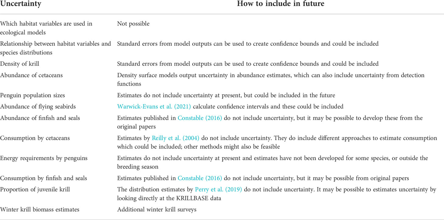
Table 2 A list of uncertainties present in each aspect of the risk assessment framework and how each may be included in future iterations. .

An initial approach to incorporating uncertainty into the risk assessment, would be to combine estimates of the high and low confidence intervals for each of the layers, and to implement the risk assessment using various combinations of these layers. To take a precautionary approach, we could combine upper confidence intervals for predator consumption with lower confidence intervals for krill density. Additionally, having an alternative idea on the distribution of krill and its impact might be a useful exercise for examining sensitivity. We suggest that further work focused on propagating uncertainty, or around reducing uncertainty would be useful.

Ecosystem dynamics

One aspect of the risk assessment framework is that the ecosystem is treated as a static snapshot, with no consideration of temporal ecosystem dynamics, other than a summer/winter assessment of risk. This is an important consideration as average ecosystem states rarely exist (Trathan et al., 2022). Nevertheless, to implement the risk assessment, it was necessary to develop data layers that reflect a spatio-temporal average for species distributions. By adopting this approach, we were unable to account for inter-annual variation in the abundance or distribution of species (stochasticity), or process error in the way these values might have been measured (uncertainty). For some predators, such as penguins and flying seabirds, it is highly likely that population numbers are generally stable across years (Humphries et al., 2017), although long-term trends in abundance do exist (Lynch et al., 2012). However, for other ecosystem components, considerable inter-annual variation exists; for example, the maximum acoustic density of krill sampled along the U.S. AMLR survey transects ranged from 827 to 6944 g m^-2 but with no long-term trend observed. Indeed, estimates of summer krill biomass were lower than the 13 year average in seven of the sampled years (Warwick-Evans et al., 2022a), potentially resulting in an underestimate of risk in those years. Fortunately, and as noted previously, our results are largely consistent with those from dynamic ecosystem models (e.g., Plagányi and Butterworth, 2012; Watters et al., 2013) that do attempt to quantify risks while the underlying abundances of species change.

One of the key processes for identifying risk involves estimating krill predation pressure. With such high inter-annual variation in krill abundance, a multi-year smooth means that there is a real possibility that in years of extreme high or low krill abundance, the index of risk is inaccurate (e.g. being too risk averse when krill abundance is high or too risk prone when krill abundance is low). It would be useful, therefore, to identify an approach by which CCAMLR could incorporate inter-annual variation in the abundance of krill in a risk-based framework, or in a yield model. Though a key concern for krill, this issue is also relevant to all data layers – reducing each species to a single layer brings with it inevitable analytical problems with increased ecological uncertainty.

Krill flux, which is the movement and retention of krill by ocean currents (Hofmann and Murphy, 2004; Thorpe et al., 2007), is also not incorporated in this static snapshot approach. Krill transportation, redistribution or replenishment after local aggregations are depleted is a key feature of the Antarctic ecosystem. It has been well established that krill are transported in ocean currents, so incorporating flux into management is an important next step. In future iterations of the risk assessment it will be important to investigate the effects of differentially weighting areas upstream and downstream of the fishery, or adding a buffer around areas important for krill reproduction, or influx into an area. For example, considering a dynamic framework that protects the major oceanographic gateways into each area preferred by the fishery might be plausible (Trathan et al., 2022). In such a scenario, estimating krill input through each gateway would allow a yield to be determined for each source, which might then be taken in the fished area. Such considerations are however for the future, as CCAMLR has agreed that initial management deliberations should not include krill flux (CCAMLR, 2018b; CCAMLR, 2021).

Measuring success

As the new krill management strategy is implemented, it is vital that monitoring occurs in all management units in which the fishery operates. We have highlighted that there are many caveats associated with this implementation of the risk assessment, and it is imperative that any unforeseen implications of these are detected at an early stage. Thus, in addition to acoustic surveys for krill at appropriate spatial and temporal scales, similar such surveys for predators should be initiated. Because the fishery will aggregate within any management zone it is likely that the risk estimated by the risk assessment will be less than experienced by the ecosystem, and catches should only be increased in line with monitoring. Initially, identifying a means of detecting any impacts of fishing on the ecosystem is essential. Subsequently, a staged approach to increasing catch limits (if the evidence indicates this is feasible) whilst monitoring impacts and reviewing management would be precautionary, and is discussed in detail in Constable (2011).

Our work suggests that a large proportion of the catch limit will be assigned to winter. As such, understanding the carryover effects into the following summer will be vital (Trathan et al., 2021).

Key questions for CCAMLR

We have identified a number of aspects that may bias the outcome of the risk assessment, and it is vital that CCAMLR address some of these issues as it proceeds with the new management strategy. Constable (2016), (Constable et al, 2002. in review) emphasised that this approach does not require perfect data but instead relies on approximating the relative risks between areas. Whilst we agree with this in principle, if the data does not adequately reflect the distribution of risk within the management area, then the outcome of the risk assessment will be biased. In particular, CCAMLR must consider how to align management with the spatial and temporal resolution at which the ecosystem operates (Watters et al., 2020). Key questions include:

● Is it ecologically meaningful to work at the seasonal (summer/winter) scale, or should alternative seasonal timescales be considered? If so, how should each season be parameterised given existing data availability?

● Do management units need to be the same for each season or can different management units be used in the winter and summer?

● How do we capture the considerable inter-annual variation in the krill-based ecosystem?

● How does CCAMLR deal with uncertainty and stochasticity?

● How does CCAMLR weight krill early-life history stages, compared with central placed foragers and pelagic predators?

Conclusions

The risk assessment framework provides a useful tool to understand the spatial and temporal scales at which to apportion krill catch limits to minimise the risks to predators and krill. The risk assessment can be updated as and when new data become available, either by survey area, season or taxon. We draw six main conclusions from the current implementation of the risk assessment for Subarea 48.1:

i. The footprint in which the fishery has operated over recent years (2013-2018) results in the highest risk to predators and krill of all of the scenarios evaluated. This means that spatial management at scales smaller than Subarea scale are now appropriate;

ii. Managing the fishery at a fine spatial scale reduces risks to krill and predators, although this may be more challenging for management procedures;

iii. In general, baseline scenarios showed lower risk estimates than when fisheries desirability was included. Given that consensus on which management units to use is most likely to be achieved using scenarios that include fisheries desirability, it is likely that CCAMLR will progress its management framework using the desirability scenarios. Options exist to offset the increase in risk if desirability scenarios are used (Constable (2016), (Constable et al, 2002. in review), but these have not yet been considered by CCAMLR;

iv. More catch is currently taken in winter, than in summer, which is consistent with proportions assigned by the risk assessment using the adjusted krill layer. As such, CCAMLR may wish to define strict seasonal allocations for catch limits, as well as spatial allocations;

v. Management units delimited using one of the variations of the U.S. AMLR krill survey strata are likely to provide a means to manage the krill fishery at a scale more closely aligned with ecosystem dynamics, with a relatively low risk to the ecosystem, whilst remaining relatively straightforward to manage. However, these still allow the fishery to aggregate and may not be appropriate if catches increase; and

vi. Inappropriate parameterisation of the risk assessment leads to erroneous estimates of risk from fishing.

The study supports earlier findings that management at scales smaller than the Subarea scale are appropriate (Watters et al., 2013; Watters et al., 2020). New data have become available and are likely to continue to do so. As such, it will be useful to update the risk assessment at regular intervals (e.g. every 5 years) to ensure that risks do not increase following any changes in the operation of the krill fishery, or changes to the ecosystem.

The overall management strategy essentially considers the ecosystem as a photographic snapshot, whereas, in reality, the ecosystem should be considered as a photographic video (Trathan et al., 2022). As CCAMLR moves forward and continues to develop the strategy into a long-term management framework, it will be important to account for certain fundamental dynamic processes within the ecosystem.

In addition to exploring the appropriate spatial scale for management units, CCAMLR will also need to remain cognizant of the tractability of implementation. The value of regional risk provides one tool that could help managers decide upon how best to choose between different scenarios with different management scales. The risk assessment provides a pragmatic approach that is tractable and transparent, providing community ownership of the management process within CCAMLR.

In this paper, we have raised a number of implementation issues that we believe CCAMLR now needs to address. However, we believe that they could all be addressed but their resolution will take further community effort. As such, we consider these risk analyses for Subarea 48.1 could be used to provide management advice in the short term, with the intention of addressing some of these issues as CCAMLR moves forward in developing a long-term management strategy.

As CCAMLR develops the risk assessment framework, it is imperative that management remains precautionary. We highlight that the existing spatial subdivision of catch offers more risk to the ecosystem than do other scenarios tested. The implications of this are that it would not be precautionary to allow catches to increase at this time, and that spatial subdivision of catches within each Subarea is now urgent. A key message for CCAMLR is that management should best occur at the same spatial and temporal scales as ecosystem function. Finally, we highlight that the endeavours reported here are the result of a community effort, demonstrating the value of common enterprise.

Data availability statement

Publicly available datasets were analyzed in this study. Data are available from the dryad data repository (doi: 10.5061/dryad.4qrfj6qc5).

Author contributions

VW-E: formal analyses (lead), methods (supporting), conception (joint lead), writing (lead) and funding (supporting). PT: conception (joint lead), methods (supporting), writing (supporting), editing and funding (lead). AC: methods (supporting), editing. LD: data provision and editing. ERS: data provision and editing. ES: data provision and editing. All authors contributed to the article and approved the submitted version.

Acknowledgments

This study is a contribution to the BAS Ecosystems programme, funded by Darwin Plus under DPLUS072, Pew Charitable Trusts under PA00034295 and the Foreign, Commonwealth and Development Office, as part of the Overseas Territories Blue Belt programme (https://www.gov.uk/government/publications/the-blue-belt-programme). The ship-based whale surveys were conducted within the activities of research projects Baleias and Interbiota, of the Brazilian Antarctic Program, financed by the National Council for Scientific and Technological Development (CNPq grant numbers 408096/2013-6 and 407889/2013-2), under the Brazilian Ministry of Science, Technology, and Innovations - MCTI. We thank all crew members of the polar vessel Almirante Maximiano, and the researchers who helped with data collection. The seabird, fur seal and krill data were collected by NOAA‐NMFS U.S. AMLR program researchers and crew on shipboard surveys during 2003‐2011; data collection and synthesis was also supported by National Science Foundation Office of Polar Programs (awards 9983751, 0337648 and 1347911). Many thanks to Natalie Kelly, Jefferson Hinke, Christian Reiss, George Watters and Dirk Welsford for their expertise and discussions about krill fishery management in Antarctica.

Conflict of interest

The authors declare that the research was conducted in the absence of any commercial or financial relationships that could be construed as a potential conflict of interest.

Publisher’s note

All claims expressed in this article are solely those of the authors and do not necessarily represent those of their affiliated organizations, or those of the publisher, the editors and the reviewers. Any product that may be evaluated in this article, or claim that may be made by its manufacturer, is not guaranteed or endorsed by the publisher.

Supplementary material

The Supplementary Material for this article can be found online at: https://www.frontiersin.org/articles/10.3389/fmars.2022.1015851/full#supplementary-material

References

Argentina and Chile (2019). Revised proposal for a conservation measure establishing a MarineProtected area in domain 1 (Western Antarctic peninsula and SouthScotia arc).

Google Scholar

Ashmole N. P. (1963). The regulation of numbers of tropical oceanic birds. Ibis 103, 458–473. doi: 10.1111/j.1474-919X.1963.tb06766.x

CrossRef Full Text | Google Scholar

Atkinson A., Hill S. L., Pakhomov E. A., Siegel V., Anadon R., Chiba S., et al. (2017). KRILLBASE: a circumpolar database of Antarctic krill and salp numerical densitie 1926–2016. Earth System Sci. Data 9, 193–210. doi: 10.5194/essd-9-193-2017

CrossRef Full Text | Google Scholar

Baines M., Jackson J. A., Fielding S., Warwick-Evans V., Reichelt M., Trathan P. (2022). Ecological interactions between Antarctic krill (Euphausia superba) and baleen whales in the south sandwich islands region – exploring predator-prey biomass ratios, in Deep Sea Res. Pt. I: Oceanog. Res. Papers. 189, 103867

Google Scholar

Boyd I. (2002). Estimating food consumption of marine predators: Antarctic fur seals and macaroni penguins. J. Appl. Ecol. 39, 103–119. doi: 10.1046/j.1365-2664.2002.00697.x

CrossRef Full Text | Google Scholar

Branch T. A. (2011). Humpback whale abundance south of 60 s from three complete circumpolar sets of surveys. J. Cetacean Res. Manage. 3, 53–69. Available at: https://journal.iwc.int/index.php/jcrm/article/view/305

Google Scholar

Burns J. M., Costa D. P., Fedak M. A., Hindell M. A., Bradshaw C. J., Gales N. J., et al. (2004). Winter habitat use and foraging behavior of crabeater seals along the Western Antarctic peninsula. Deep Sea Res. Part II: Topical Stud. Oceanography 51, 2279–2303. doi: 10.1016/j.dsr2.2004.07.021

CrossRef Full Text | Google Scholar

Calderan S. V., Black A., Branch T. A., Collins M. A., Kelly N., Leaper R., et al. (2020). South Georgia blue whales five decades after the end of whaling. Endangered Species Res. 43, 359–373. doi: 10.3354/esr01077

CrossRef Full Text | Google Scholar

CCAMLR. (2013). (Hobart, Australia: CCAMLR). Available at: https://www.ccamlr.org/en/organisation/camlr-convention-text.

Google Scholar

CCAMLR. (2016) Conservation measure 51-07 (Hobart, Australia: CCAMLR). Available at: https://cm.ccamlr.org/en/measure-51-07-2016?check_logged_in=1.

Google Scholar

CCAMLR. (2018a) Krill fishery report. (Hobart, Australia: CCAMLR) Available at: https://www.ccamlr.org/en/document/publications/krill-fishery-report-2018.

Google Scholar

CCAMLR. (2018b). Report of the working group on ecosystem monitoring and management.

Google Scholar

CCAMLR. (2019). “Scientific committee for the conservation of Antarctic marine living resources,” in Report of the thirty-eighth meeting of the scientific committee. (Hobart, Australia: CCAMLR).

Google Scholar

CCAMLR. (2021). Report of the working group on acoustic survey and analysis methods. (Hobart, Australia: CCAMLR).

Google Scholar

Clarke A. (1980). The biochemical composition of krill, euphausia superba Dana, from south Georgia. J. Exp. Mar. Biol. Ecol. 43, 221–236. doi: 10.1016/0022-0981(80)90049-0

CrossRef Full Text | Google Scholar

Constable A. J. (2002). CCAMLR ecosystem monitoring and management: future work. CCAMLR Sci. 9, 233–253.

Google Scholar

Constable A. J. (2011). Lessons from CCAMLR on the implementation of the ecosystem approach to managing fisheries. Fish Fish. 12, 138–151. doi: 10.1111/j.1467-2979.2011.00410.x

CrossRef Full Text | Google Scholar

Constable A. (2016). “E-group on CM-51-07 WG-EMM review. 2016. scientific contribution to the 2016 review of conservation measure 51-07,” in Part 1 – rationale, method and data for a risk assessment ramework for distributing the krill trigger level.

Google Scholar

Constable A., Kawaguchi S., Sumner M., Trathan P., Warwick-Evans V. (in review) Rationale, method and data for a risk assessment ramework for distributing the krill trigger level. Front. Mar. Sci.

Google Scholar

Croll D., Tershy B. (1998). Penguins, fur seals, and fishing: prey requirements and potential competition in the south Shetland islands, Antarctica. Polar Biol. 19, 365–374. doi: 10.1007/s003000050261

CrossRef Full Text | Google Scholar

Croxall J. P., Prince P., Ricketts C. (1985). “Relationships between prey life-cycles and the extent, nature and timing of seal and seabird predation in the Scotia Sea,” in Antarctic Nutrient cycles and food webs (Berlin, Heidelberg: Springer), 516–533.

Google Scholar

Croxall J., Reid K., Prince P. (1999). Diet, provisioning and productivity responses of marine predators to differences in availability of Antarctic krill. Mar. Ecol. Prog. Ser. 177, 115–131. doi: 10.3354/meps177115

CrossRef Full Text | Google Scholar

Curtice C., Johnston D. W., Ducklow H., Gales N., Halpin P. N., Friedlaender A. S. (2015). Modeling the spatial and temporal dynamics of foraging movements of humpback whales (Megaptera novaeangliae) in the Western Antarctic peninsula. Movement Ecol. 3, 1–9. doi: 10.1186/s40462-015-0041-x

CrossRef Full Text | Google Scholar

Dalla Rosa L., Secchi E., Maia Y., Zerbini A., Heide-Jørgensen M. (2008). Movements of satellite-monitored humpback whales on their feeding ground along the Antarctic peninsula. Polar Biol. 31, 771–781. doi: 10.1007/s00300-008-0415-2

CrossRef Full Text | Google Scholar

Daniels R. A. (1978). Nesting behaviour of harpagifer bispinis in Arthur harbour, Antarctic peninsula. J. Fish Biol. 12, 465–474. doi: 10.1111/j.1095-8649.1978.tb04190.x

CrossRef Full Text | Google Scholar

Ekstrom P. A. (2004). An advance in geolocation by light. (National Institute of Polar Research)

Google Scholar

Emmerson L., Southwell C. (2017). Estimating prey consumption of the non-breeder component of an adélie penguin population (WG-EMM). (Hobart, Australia: CCAMLR).

Google Scholar

Erdmann E. S., Ribic C. A., Patterson-Fraser D. L., Fraser W. R. (2011). Characterization of winter foraging locations of adélie penguins along the Western Antarctic peninsula 2001–2002. Deep Sea Res. Part II: Topical Stud. Oceanography 58, 1710–1718. doi: 10.1016/j.dsr2.2010.10.054

CrossRef Full Text | Google Scholar

Forcada J., Trathan P. N., Boveng P. L., Boyd I. L., Burns J. M., Costa D. P., et al. (2012). Responses of Antarctic pack-ice seals to environmental change and increasing krill fishing. Biol. Conserv. 149, 40–50. doi: 10.1016/j.biocon.2012.02.002

CrossRef Full Text | Google Scholar

Godø O. R., Trathan P. (2022). Voluntary actions by the Antarctic krill fishing industry help reduce potential negative impacts on land-based marine predators during breeding, highlighting the need for CCAMLR action. ICES J. Mar. Sci. 79 (5), 1457–1466. doi: 10.1093/icesjms/fsac092

CrossRef Full Text | Google Scholar

Hewitt R., Watters G., Trathan P., Croxall J., Goebel M. E., Ramm D., et al. (2004). Options for allocating the precautionary catch limit of krill among small-scale management units in the Scotia Sea. CCAMLR Sci. 11, 81–97.

Google Scholar

Hill S., Reid K., Thorpe S. E., Hinke J. T., Watters G. M. (2007). A compilation of parameters for ecosystem dynamics models of the Scotia Sea–Antarctic peninsula region. CCAMLR Sci. 14, 1–25.

Google Scholar

Hinke J. T., Cossio A. M., Goebel M. E., Reiss C. S., Trivelpiece W. Z., Watters G. M. (2017). Identifying risk: concurrent overlap of the Antarctic krill fishery with krill-dependent predators in the Scotia Sea. PloS One 12, e0170132. doi: 10.1371/journal.pone.0170132

PubMed Abstract | CrossRef Full Text | Google Scholar

Hinke J. T., Polito M. J., Goebel M. E., Jarvis S., Reiss C. S., Thorrold S. R., et al. (2015). Spatial and isotopic niche partitioning during winter in chinstrap and adélie penguins from the south Shetland islands. Ecosphere 6, 1–32. doi: 10.1890/ES14-00287.1

CrossRef Full Text | Google Scholar

Hinke J. T., Salwicka K., Trivelpiece S. G., Watters G. M., Trivelpiece W. Z. (2007). Divergent responses of pygoscelis penguins reveal a common environmental driver. Oecologia 153, 845. doi: 10.1007/s00442-007-0781-4

PubMed Abstract | CrossRef Full Text | Google Scholar

Hinke J. T., Santos M. M., Korczak-Abshire M., Milinevsky G., Watters G. M. (2019). Individual variation in migratory movements of chinstrap penguins leads to widespread occupancy of ice-free winter habitats over the continental shelf and deep ocean basins of the southern ocean. PloS One 14. doi: 10.1371/journal.pone.0226207

CrossRef Full Text | Google Scholar

Hinke J. T., Trivelpiece W. Z. (2011). Daily activity and minimum food requirements during winter for gentoo penguins (Pygoscelis papua) in the south Shetland islands, Antarctica. Polar Biol. 34, 1579–1590. doi: 10.1007/s00300-011-1018-x

CrossRef Full Text | Google Scholar

Hofmann E. E., Murphy E. J. (2004). Advection, krill, and Antarctic marine ecosystems. Antarctic Sci. 16, 487–499. doi: 10.1017/S0954102004002275

CrossRef Full Text | Google Scholar

Hückstädt L. A., Piñones A., Palacios D. M., McDonald B. I., Dinniman M. S., Hofmann E. E., et al. (2020). Projected shifts in the foraging habitat of crabeater seals along the Antarctic peninsula. Nat. Climate Change 10, 472–477. doi: 10.1038/s41558-020-0745-9

CrossRef Full Text | Google Scholar

Humphries G., Naveen R., Schwaller M., Che-Castaldo C., McDowall P., Schrimpf M., et al. (2017). Mapping application for penguin populations and projected dynamics (MAPPPD): Data and tools for dynamic management and decision support. Polar Rec. 53, 160–166. doi: 10.1017/S0032247417000055

CrossRef Full Text | Google Scholar

Jackson J. A., Ross-Gillespie A., Butterworth D., Findlay K., Holloway S., Robbins J., et al. (2015). “Southern hemisphere humpback whale comprehensive assessment. a synthesis and summary: 2005-2015,” in Report to the scientific committee of the international whaling commission. (Cambridge, UK: IWC)

Google Scholar

Kawaguchi S., Nicol S. (2020). Krill fishery. Fish. Aquacult, 137–158. doi: 10.1093/oso/9780190865627.003.0006

CrossRef Full Text | Google Scholar

Kelly N., Emmerson L., Kawaguchi S., Southwell C., Welsford D. (2018). “An ecological risk assessment of current conversation measures for krill fishing in East Antarctica,” in Ecosystem monitoring and management working group, vol. 18/37. (Hobart, Australia: CCAMLR), 27.

Google Scholar

Klein E. S., Watters G. M. (2020). What’s the catch? profiling the benefits and costs associated with marine protected areas and displaced fishing in the Scotia Sea. PloS One 15, e0237425. doi: 10.1371/journal.pone.0237425

PubMed Abstract | CrossRef Full Text | Google Scholar

Krafft B. A., Krag L. A., Engås A., Nordrum S., Bruheim I., Herrmann B. (2016). Quantifying the escape mortality of trawl caught Antarctic krill (Euphausia superba). PloS One 11, e0162311. doi: 10.1371/journal.pone.0162311

PubMed Abstract | CrossRef Full Text | Google Scholar

Krüger L. (2019). Spatio-temporal trends of the krill fisheries in the Western Antarctic peninsula and southern Scotia arc. Fish. Manage. Ecol. 26, 327–333. doi: 10.1111/fme.12363

CrossRef Full Text | Google Scholar

Lascara C. M., Hofmann E. E., Ross R. M., Quetin L. B. (1999). Seasonal variability in the distribution of Antarctic krill, euphausia superba, west of the Antarctic peninsula. Deep Sea Res. Part I: Oceanographic Res. Papers 46, 951–984. doi: 10.1016/so967-0637(98)00099-5

CrossRef Full Text | Google Scholar

Leaper R., Miller C. E. (2011). Management of Antarctic baleen whales amid past exploitation, current threats and complex marine ecosystems. Antarctic Sci. 23, 503–529. doi: 10.1017/S0954102011000708

CrossRef Full Text | Google Scholar

Lockyer C. (1981). Growth and energy budgets of large baleen whales from the Southern Hemisphere, in Food Agri. Org. 3, 379–487.

Google Scholar

Lynch H. J., Naveen R., Trathan P. N., Fagan W. F. (2012). Spatially integrated assessment reveals widespread changes in penguin populations on the Antarctic peninsula. Ecology 93, 1367–1377. doi: 10.1890/11-1588.1

PubMed Abstract | CrossRef Full Text | Google Scholar

Meyer B., Atkinson A., Bernard K. S., Brierley A. S., Driscoll R., Hill S. L., et al. (2020). Successful ecosystem-based management of Antarctic krill should address uncertainties in krill recruitment, behaviour and ecological adaptation. Commun. Earth Environ. 1, 1–12. doi: 10.1038/s43247-020-00026-1

CrossRef Full Text | Google Scholar

Nowacek D. P., Friedlaender A. S., Halpin P. N., Hazen E. L., Johnston D. W., Read A. J., et al. (2011). Super-aggregations of krill and humpback whales in Wilhelmina bay, Antarctic peninsula. PloS One 6. doi: 10.1371/journal.pone.0019173

CrossRef Full Text | Google Scholar

Orians G. H., Pearson N. E. (1979). “On the theory of central place foraging,” in Analysis of ecological systems (Columbus: Ohio State University Press), 155–177.

Google Scholar

Perry F. A., Atkinson A., Sailley S. F., Tarling G. A., Hill S. L., Lucas C. H., et al. (2019). Habitat partitioning in Antarctic krill: Spawning hotspots and nursery areas. PloS One 14, e0219325. doi: 10.1371/journal.pone.0219325

PubMed Abstract | CrossRef Full Text | Google Scholar

Pew (2020) The need for a network of marine protected areas in the southern ocean. Available at: https://www.pewtrusts.org/en/research-and-analysis/issue-briefs/2020/10/the-need-for-a-network-of-marine-protected-areas-in-the-southern-ocean (Accessed 04/07/2022).

Google Scholar

Plagányi É. E., Butterworth D. S. (2012). The Scotia Sea krill fishery and its possible impacts on dependent predators: modeling localized depletion of prey. Ecol. Appl. 22, 748–761. doi: 10.1890/11-0441.1

PubMed Abstract | CrossRef Full Text | Google Scholar

R Core Team. (2022). R: A language and environment for statistical computing (Vienna, Austria: R Foundation for Statistical Computing). Available at: https://www.R-project.org/.

Google Scholar

Reid K., Watkins J. L., Murphy E. J., Trathan P. N., Fielding S., Enderlein P. (2010). Krill population dynamics at south Georgia: Implications for ecosystem-based fisheries management. Mar. Ecol. Prog. Ser. 399, 243–252.

Google Scholar

Reilly S., Hedley S., Borberg J., Hewitt R., Thiele D., Watkins J., et al. (2004). Biomass and energy transfer to baleen whales in the south Atlantic sector of the southern ocean. Deep Sea Res. Part II: Topical Stud. Oceanography 51, 1397–1409. doi: 10.1016/j.dsr2.2004.06.008

CrossRef Full Text | Google Scholar

Reiss C. S., Cossio A. M., Loeb V., Demer D. A. (2008). Variations in the biomass of Antarctic krill (Euphausia superba) around the south Shetland islands 1996–2006. ICES J. Mar. Sci. 65, 497–508. doi: 10.1093/icesjms/fsn033

CrossRef Full Text | Google Scholar

Reiss C. S., Cossio A., Santora J. A., Dietrich K. S., Murray A., Mitchell B. G., et al. (2017). Overwinter habitat selection by Antarctic krill under varying sea-ice conditions: implications for top predators and fishery management. Mar. Ecol. Prog. Ser. 568, 1–16.

Google Scholar

Santa Cruz F., Ernst B., Arata J. A., Parada C. (2018). Spatial and temporal dynamics of the Antarctic krill fishery in fishing hotspots in the bransfield strait and south Shetland islands. Fish. Res. 208, 157–166. doi: 10.1016/j.fishres.2018.07.020

CrossRef Full Text | Google Scholar

Santa Cruz F., Krüger L., Cárdenas C. A. (2022). Spatial and temporal catch concentrations for Antarctic krill: Implications for fishing performance and precautionary management in the southern ocean. Ocean Coast. Manage. 223, 106146. doi: 10.1016/j.ocecoaman.2022.106146

CrossRef Full Text | Google Scholar

Savoca M. S., Czapanskiy M. F., Kahane-Rapport S. R., Gough W. T., Fahlbusch J. A., Bierlich K., et al. (2021). Baleen whale prey consumption based on high-resolution foraging measurements. Nature 599, 85–90. doi: 10.1038/s41586-021-03991-5

PubMed Abstract | CrossRef Full Text | Google Scholar

Saunders R. A., Brierley A. S., Watkins J. L., Reid K., Murphy E. J., Enderlein P., et al. (2007). Intra-annual variability in the density of Antarctic krill (Euphausia superba) at south Georgia, 2002–2005: within-year variation provides a new framework for interpreting previous ‘annual’estimates of krill density. CCAMLR Sci. 14, 27–41.

Google Scholar

SC-CCAMLR-XXI (2002). Report of the twenty-first meeting of the scientific committee, annex 4, appendix d: Report of the workshop on small-scale management units, such as predator units (Hobart, Australia: Commission for the Conservation of Antarctic Marine Living Resources).

Google Scholar

Shaffer S. A. (2011). A review of seabird energetics using the doubly labeled water method. Comp. Biochem. Physiol. Part A: Mol. Integr. Physiol. 158, 315–322. doi: 10.1016/j.cbpa.2010.07.012

CrossRef Full Text | Google Scholar

Silk J., Hill S., Trathan P. (2014). Exploring variability in the locations used by the krill fishery in area 48 in relation to intra-and inter-annual variability in seasonal sea ice (Punta Arenas, Chile: CCAMLR Working Group on Ecosystem Monitoring and Management).

Google Scholar

Širović A., Hildebrand J. A., Wiggins S. M., McDonald M. A., Moore S. E., Thiele D. (2004). Seasonality of blue and fin whale calls and the influence of sea ice in the Western Antarctic peninsula. Deep Sea Res. Part II: Topical Stud. Oceanography 51, 2327–2344. doi: 10.1016/j.dsr2.2004.08.005

CrossRef Full Text | Google Scholar

Southwell D., Emmerson L., Forcada J., Southwell C. (2015). A bioenergetics model for estimating prey consumption by an adélie penguin population in East Antarctica. Mar. Ecol. Prog. Ser. 526, 183–197. doi: 10.3354/meps11182

CrossRef Full Text | Google Scholar

Strycker N., Wethington M., Borowicz A., Forrest S., Witharana C., Hart T., et al. (2020). A global population assessment of the chinstrap penguin (Pygoscelis antarctica). Sci. Rep. 10, 1–11. doi: 10.1038/s41598-020-76479-3

PubMed Abstract | CrossRef Full Text | Google Scholar

Tanton J. L., Reid K., Croxall J. P., Trathan P. N. (2004). Winter distribution and behaviour of gentoo penguins pygoscelis papua at south Georgia. Polar Biol. 27, 299–303. doi: 10.1007/s00300-004-0592-6

CrossRef Full Text | Google Scholar

Thorpe S., Murphy E., Watkins J. (2007). Circumpolar connections between Antarctic krill (Euphausia superba Dana) populations: investigating the roles of ocean and sea ice transport. Deep Sea Res. Part I: Oceanographic Res. Papers 54, 792–810. doi: 10.1016/j.dsr.2007.01.008

CrossRef Full Text | Google Scholar

Tranter D. (1982). Interlinking of physical and biological processes in the Antarctic ocean. Oceanography Mar. Biol. 20, 9.

Google Scholar

Trathan P., Fielding S., Hollyman P., Murphy E., Warwick-Evans V., Collins M. (2021). Enhancing the ecosystem approach for the fishery for Antarctic krill within the complex, variable and changing ecosystem at south Georgia. ICES J. Mar. Sci. 78 (6), 2065–2081. . doi: 10.1093/icesjms/fsab092

CrossRef Full Text | Google Scholar

Trathan P., Lynch H. J., Fraser W. (2019). Changes in penguin distribution over the Antarctic peninsula and Scotia arc. Antarctic Environments Portal. doi: 10.18124/chrj-g976

CrossRef Full Text | Google Scholar

Trathan P. N., Warwick-Evans V., Hinke J., Young E. F., Murphy E. J., Carneiro A., et al. (2018). Managing fishery development in sensitive ecosystems: identifying penguin habitat use to direct management in Antarctica. Ecosphere 9. doi: 10.1002/ecs2.2392

CrossRef Full Text | Google Scholar

Trathan P., Warwick-Evans V., Young E. F., Friedlaender A. S., Kim J.-H., Kokubun N. (2022). The ecosystem approach to management of the Antarctic krill fishery - the ‘devils are in the detail’ at small spatial and temporal scales. J. Mar. Syst. 225, 103598doi: 10.1016/j.jmarsys.2021.103598

CrossRef Full Text | Google Scholar

Veytia D., Corney S., Meiners K. M., Kawaguchi S., Murphy E. J., Bestley S. (2020). Circumpolar projections of Antarctic krill growth potential. Nat. Climate Change 10 (6), 1–8. doi: 10.1038/s41558-020-0758-4

CrossRef Full Text | Google Scholar

Warwick-Evans V., Downie R., Santos M., Trathan P. N. (2019). Habitat preferences of adélie pygoscelis adeliae and chinstrap penguins pygoscelis antarctica during pre-moult in the weddell Sea (Southern ocean). Polar Biol. 42, 703–714. doi: 10.1007/s00300-019-02465-9

CrossRef Full Text | Google Scholar

Warwick-Evans V., Fielding S., Reiss C., Watters G., Trathan P. (2022a). Estimating the average distribution of Antarctic krill at the northern Antarctic peninsula during austral summer and winter. Polar Biol. 45, 857–871. doi: 10.1007/s00300-022-03039-y

PubMed Abstract | CrossRef Full Text | Google Scholar

Warwick-Evans V., Kelly N., dalla Rosa L., Friedlaender A. S., Hinke J., Kim J.-H., et al. (2022b). Using seabird and whale distribution models to estimate spatial consumption of krill to inform fishery management. Ecosphere. 13 (6), e4083. doi: 10.1002/ecs2.4083

CrossRef Full Text | Google Scholar

Warwick-Evans V., Ratcliffe N., Lowther A. D., Manco F., Ireland L., Clewlow H. L., et al. (2018). Using habitat models for chinstrap penguins pygoscelis antarctica to advise krill fisheries management during the penguin breeding season. Diversity Distributions 24, 1756–1771. doi: 10.1111/ddi.12817

CrossRef Full Text | Google Scholar

Warwick-Evans V., Santora J. A., Waggitt J. J., Trathan P. N., Votier S. (2021). Multi-scale assessment of distribution and density of procellariiform seabirds within the northern Antarctic peninsula marine ecosystem. ICES J. Mar. Sci. 78, 1324–1339. doi: 10.1093/icesjms/fsab020

CrossRef Full Text | Google Scholar

Watters G., Hewitt R. (1992). Alternative methods for determining subarea or local area catch limits for krill in statistical area 48. (Hobart, Australia: CCAMLR).

Google Scholar

Watters G. M., Hill S., Hinke J., Matthews J., Reid K. (2013). Decision-making for ecosystem-based management: evaluating options for a krill fishery with an ecosystem dynamics model. Ecol. Appl. 23, 710–725. doi: 10.1890/12-1371.1

PubMed Abstract | CrossRef Full Text | Google Scholar

Watters G., Hill S. L., Hinke J., Trathan P. (2009). The risks of not deciding to allocate the precautionary krill catch limit among SSMUs and allowing uncontrolled expansion of the krill fishery up to the trigger level. (Hobart, Australia: CCAMLR).

Google Scholar

Watters G. M., Hinke J. T., Reiss C. S. (2020). Long-term observations from Antarctica demonstrate that mismatched scales of fisheries management and predator-prey interaction lead to erroneous conclusions about precaution. Sci. Rep. 10, 1–9. doi: 10.1038/s41598-020-59223-9

PubMed Abstract | CrossRef Full Text | Google Scholar

Weinstein B. G., Friedlaender A. S. (2017). Dynamic foraging of a top predator in a seasonal polar marine environment. Oecologia 185, 427–435. doi: 10.1007/s00442-017-3949-6

PubMed Abstract | CrossRef Full Text | Google Scholar