Identifying seasonal distribution patterns of fin whales across the Scotia Sea and the Antarctic Peninsula region using a novel approach combining habitat suitability models and ensemble learning methods

1. Introduction

Southern Hemisphere fin whales (Balaenoptera physalus quoyi, SHFW) were the most numerously exploited whale species in the Southern Ocean during 20th century industrial whaling, with over 700,000 individuals killed (Clapham and Baker, 2002). Today, the current population status of SHFW is unknown, and knowledge about the spatio-temporal distribution of SHFW is limited (Leaper and Miller, 2011; Edwards et al., 2015). In their world-wide assessment of fin whale distribution, (Edwards et al., 2015) identified the Southern Hemisphere as a data gap region. SHFW are assumed to be extensively distributed in latitudes between 40°S and 60°S, and rare to absent in equatorial waters north of 20°S and in the ice-covered waters south of 60°S (Edwards et al., 2015; Cooke, 2018). Like most balaenopterids, their general migratory pattern presumably is a movement between poleward feeding areas in the summer months and lower latitudes in the winter months (Mackintosh, 1966; Mizroch et al., 1984). However, foraging areas have also been identified at low latitudes (Pérez et al., 2006; Toro et al., 2016; Sepúlveda et al., 2018). Migratory routes and the locations of Southern Hemisphere breeding grounds have not yet been identified (Mizroch et al., 1984; Edwards et al., 2015; Cooke, 2018) and SHFW population structure is not yet fully understood (Archer et al., 2013; Archer et al., 2019; Cabrera et al., 2019; Pérez-Alvarez et al., 2021; Wood and Širović, 2022).

Today, much of the understanding of circumpolar post-whaling distribution and abundance of whales is based on the International Whaling Commission’s (IWC) International Decade of Cetacean Research (IDCR) and Southern Ocean Whale Ecosystem Research (SOWER) cruise programmes, carried out in three circumpolar sets of surveys between 1978 and 2004, and localised ‘experimental’ voyages until 2010. Based on IDCR/SOWER data from surveys between 1991 and 1998, circumpolar fin whale abundance south of 60°S was last estimated at 5,445 individuals (95% CI 2,000–14,500) (Branch and Butterworth, 2001). However, since some uncertain, but potentially substantial, proportion of the population may range north of 60°S during the summer months, surveyed areas did not represent their complete summer distribution, therefore, this estimate probably under-represents the total population size. For the Scotia Arc and Antarctic Peninsula region, the last SHFW abundance estimate is 4,672 (CV 42.37) based on data from the dedicated CCAMLR/SOWER 2000 survey conducted in February and March 2000 (Reilly et al., 2004). Dedicated surveys to estimate abundance have also been carried out for small discrete regions around the Antarctic Peninsula (Herr et al., 2016; Viquerat and Herr, 2017; Herr et al., 2022).

High densities and large feeding aggregations of fin whales have been reported from the Western Antarctic Peninsula (WAP) in the past decade (Santora et al., 2010; Santora et al., 2014; Herr et al., 2016; Viquerat and Herr, 2017; Herr et al., 2022), indicating that some level of post-whaling population recovery has begun (Herr et al., 2022). Systematic surveys targeting fin whale distribution in the Atlantic sector of the Southern Ocean, including areas north of 60°S, are not yet available. However, in addition to smaller scale dedicated surveys, data on fin whale occurrences have been collected opportunistically during research and commercial expeditions over the past few decades, incorporating both Antarctic and sub-Antarctic latitudes. These datasets are held by a variety of different organisations and data holders. Combining these disparate data into a single comprehensive analysis, these datasets represent a source of information on the seasonality, distribution and abundance of SHFWs.

The main objective of this study was to predict the distribution of fin whales in time and space across the Antarctic Peninsula and Scotia Sea region using biological and environmental data as predictors. To achieve this, we (i) compiled sighting records of SHFW from the Antarctic Peninsula and Scotia Sea region from multiple sources and research groups; (ii) used an ensemble learning and a maximum entropy approach to develop a workflow to estimate a minimum abundance from non-standardised opportunistically collected datasets; and (iii) provide insight into the environmental correlates that may be associated with the seasonality and distribution of SHFW across the Antarctic Peninsula and Scotia Sea region across a 40-year period.

2. Material and methods

2.1. Data integration and preparation

We compiled SHFW sighting records from datasets of ten different data holders (Table 1; Table S1 for a detailed table including all references for the data set and Figure S1 for a map of all records by providers). In addition, we sourced data from two mass online repositories (GBIF.org and OBIS.org; accessed on the 6^th of April 2021) for all SHFW records. In order to deal with the potential redundancy with the mass online data repositories, we excluded all duplicates based on location (geographic coordinates rounded to 2 digits), year and month, keeping the data that were submitted to us by data holders. Data were restricted to records south of 50°S and between 90°W and 10°W. We only used definite fin whale sightings and excluded fin-like type of sightings and any other identification with uncertain species identification. Sighting records from non-scientific personnel were based on photographic evidence. All definite fin whale records were considered confirmed presences. Data sets in this study originated from dedicated surveys for marine mammals and from opportunistic collection of sightings. Of these, only dedicated survey data sets provided information on search effort. We used stretches of survey effort without fin whale detections from dedicated surveys as pseudo absence records [‘pseudo’, because absences in marine mammal surveys can never be considered ‘true’ absences (Barlow, 2015; Hammond et al., 2021)]. All geographic information was projected to IBCSO projection (EPSG: 9345; https://epsg.org/crs_9354/WGS-84-IBCSO-Polar-Stereographic.html). The pooled dataset contained the geographic position, estimated group size (including information on number of groups detected and the number of animals; for pseudo absences = 0), the year and the month for each presence/pseudo absence record.

TABLE 1

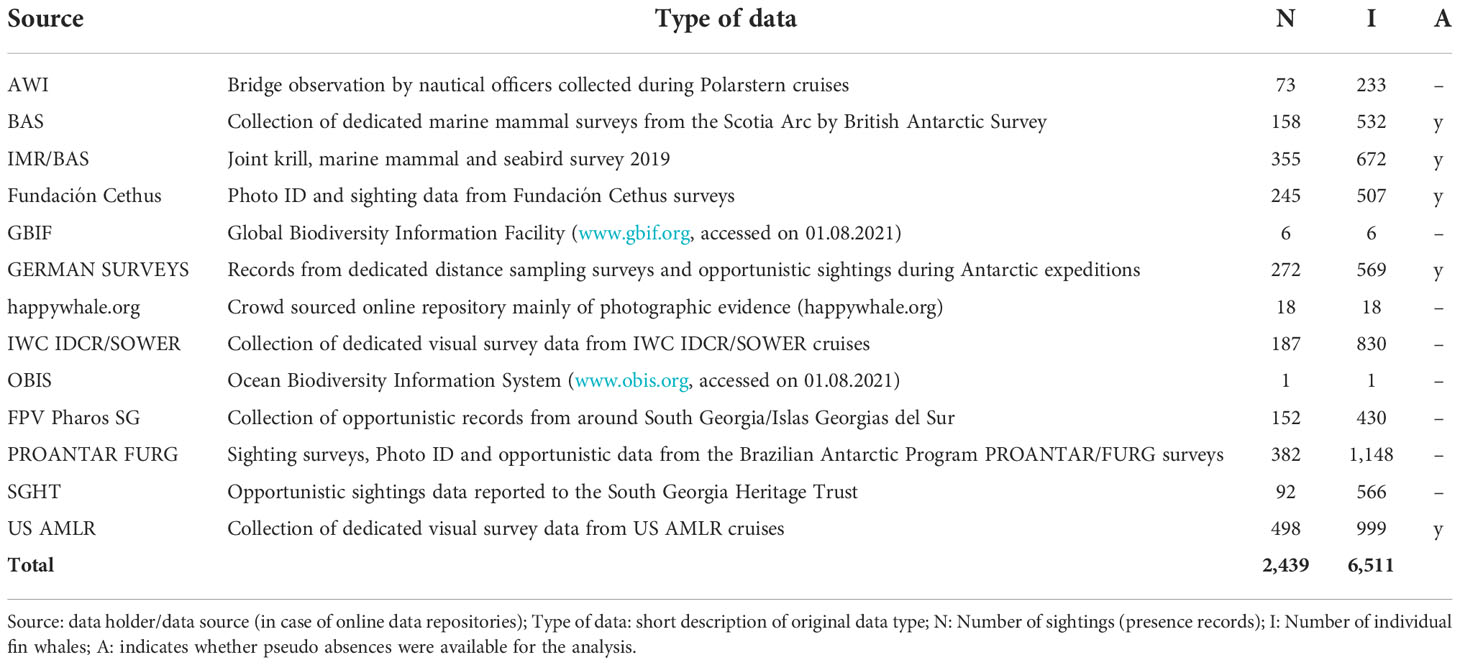
Table 1 Summary of data sources and number of provided records.

We only considered data recorded after the introduction of the IWC’s New Management Procedure (International Whaling Commision, 1976) when all SHFW were classified as Protection Stocks in 1976, setting the quota in the Southern Hemisphere to zero (International Whaling Commision, 1978), i.e., marking the end of commercial whaling on fin whales. Therefore, the dataset starts with the first dedicated large whale survey in the Southern Ocean (IDCR/SOWER) in 1978 and concludes with the PHAROS surveys in January 2021. We pooled data across years into seasonal quarters (at regular three-month intervals, i.e. Q1: January – March, Q2: April – June, Q3: July – September and Q4: October – December).

2.2. Creation of sample grids

We based the boundary of our analysis on a convex hull around all presence records of the data set. This area was extended by 100 km in order to include the neighbouring environment for records near the boundary line. The Antarctic Sound and the waters surrounding the Weddell Sea were manually excluded from the analysis due to data sparsity. The spatial extent of our study area comprised data within 80°W to 17°W and 50°S to 70°S, respectively, covering an area of app. 5.2 x 10⁶ km².

We selected a set of nine candidate static and environmental covariates based on their perceived ecological relevance for cetaceans [e.g. (Sagnol et al., 2014; Claro et al., 2020)], which were available across the extent of the survey area (Table 2). The majority of static covariates used in this analysis originates from depth data, for which we used the International Bathymetric Chart of the Southern Ocean, version 2 [IBCSO v2 (Dorschel et al., 2022)]. Slope, aspect (the direction that the slope is facing), topographic position index (tpi; a measure used to classify the structure of an area surrounding a point) and terrain ruggedness index [tri; quantifying the variability of elevation (Riley et al., 1999)] were calculated using the terrain function from the raster package (Hijmans, 2017) in R 4.0.4 (R Core Team, 2021). The implementation of tpi and tri followed (Wilson et al., 2007). These seafloor features describe physical properties that in turn may impact the ecological value of an area of ocean and are therefore prime candidates for species distribution studies in the Southern Ocean (El-Gabbas et al., 2021a; El-Gabbas et al., 2021b; Reisinger et al., 2021) and elsewhere (Díaz López and Methion, 2019; Claro et al., 2020). We calculated the absolute distance from the continental shelf break (using the shelf break as detected in (Herr et al., 2019) using spatial samples at a regular 5 km intervals via spsample in R version 4.0.4 and produced a regular grid with each cell containing the distance to the nearest shelf edge line. For the set of dynamic covariates, we extracted monthly averages of sea surface temperature (sst) and chlorophyll-α (chla) for each year (starting from 2002) from https://neo.sci.gsfc.nasa.gov/archive/geotiff.float/MY1DMM_CHLORA/(chla) and https://neo.sci.gsfc.nasa.gov/archive/geotiff.float/MYD28M/(sst) and used these as environmental covariates. For data collected prior to 2002, monthly averages from later years were used as a rough approximation for sst and chla. All covariates were resampled to a regular grid of 5x5km resolution and projected to IBCSO (EPSG: 9354) to facilitate the analysis.

TABLE 2

Table 2 Description of variables used in the analysis.

We subdivided our study area into regular hexagonal polygon cells with a grid spacing of 20 km, leading to a regular and equidistant grid of approximately 320 km² cells. We extracted the static and environmental covariates to each grid cell based on the median of the respective covariate grid for each cell and separately for each quarter.

All fin whale records (both presence and pseudo absences) were aggregated to the grid cells for each seasonal quarter, respectively, resulting in four seasonal sample grids containing all covariates and a summary of fin whale records and pseudo absences pooled across 1978 – 2021 (see Figure 2). Each seasonal sample grid contained information on the grid centroid (i.e. the midpoint coordinates of the hex cell), the observed number of fin whales, the number of fin whale groups and the average group size per grid cell (where available) for the respective seasonal quarter. We assigned presence and pseudo absence per sample grid cell based on the observed number of fin whale groups, adhering to the following rules:

Presence within a seasonal quarter and cell supersedes pseudo absence – Since absences in marine mammals can never be considered ‘true’ absences with certainty (hence the term ‘pseudo absence’), any confirmed presence superseded pseudo absence. All pseudo absences from a seasonal quarter that were assigned to a cell that was also associated with a presence record for the given seasonal quarter were therefore discarded for this analysis.

Multiple pseudo absence records within a seasonal quarter and cell were treated as a single record of pseudo absence – During dedicated surveys, effort is recorded at discrete intervals. Any number of pseudo absence records within a cell was therefore treated as a single record of absence.

2.3. Stratification of survey area

In order to quantify fin whale numbers, we selected four sub areas within the study area that provided a robust sample size (i.e. good coverage across at least some quarters). We centred these on four distinct island groups within the study area and named them accordingly: (i) South Georgia (Islas Georgias del Sur), (ii) South Orkney Islands, (iii) Elephant Island, and (iv) South Shetland Islands (Figure 3).

2.4. Analysis

We checked for the spatial auto correlation of our sample grid data using Moran’s I (Moran, 1950) in ape (Paradis et al., 2018), noting any covariates that were spatially auto correlated. In addition, we ran separate correlation tests per quarter based on Spearman’s ρ, ρ² and a hierarchical clustering on variables (using Spearman’s ρ² as distance metric) in Hmisc (Harrell, 2018) in R version 4.0.4 (R Core Team, 2021). We used a threshold of ρ² = 0.5 to decide which covariates to keep. For each quarter, we assessed whether covariates are feasible based on these metrics. If a covariate showed signs of collinearity or correlation, it was rejected as a potential covariate for the analysis of respective quarter (Figures S2–S5).

The model framework in this study can be summarised in three steps: (1) fitting a species distribution model (SDM) to obtain the spatial distribution of presence probabilities, (2) fitting a random forest model using generalized least squares (RF-GLS) to predict the spatial distribution of fin whale group sizes and (3) combining the results of the SDM and RF-GLS step to produce minimum abundance estimates for each of the Island Groups.

2.4.1. Species distribution model

We estimated the probability of presence of fin whales within the survey area per quarter with a maximum entropy approach (Phillips et al., 2020) as implemented in maxent version 3.4.0 (http://biodiversityinformatics.amnh.org/open_source/maxent) via the dismo package (Hijmans et al., 2017) in R. Each model ran 100 replicates using bootstrapping for sample selection within each replicate. We used the spatially thinned data in the sample grid as input data for the modelling step, with each presence cell entering the model as an occurrence point (using cell midpoints as location) and each pseudo absence cell as a background point (if available). For each seasonal quarter, we tested the same set of models. As environmental data on sst and chla were not available in sufficient quality for Q2 (April – June) and Q3 (July – September), models containing environmental covariates were only run for Q1 and Q4 (October-December). All models containing covariates that were discarded either due to spatial autocorrelation or collinearity with other model terms were skipped. Model diagnostics for each replicate were extracted using the evaluate function in dismo (Hijmans et al., 2017).

Due to the high number of diagnostic measures and model replicates, we chose a dimension reduction approach, condensing the number of diagnostic measures for each model and quarters onto two principal component axes (each therefore giving the relative importance of its loadings). This allowed for visual model comparison, including the variability between replicates of a model and variability between models. The final selection of the best model for each season was based on the area under the curve (AUC; summarising the ratio of true positive rate and false negative rate with AUC values close to 1 indicating excellent models and values close to 0 indicating inadequate models) and Cohen’s Kappa (Liu et al., 2011). The selected model for each quarter was re-run with the same data, number of replicates and maxent settings (this was necessary due to computational limitations, as we could not store all model replicates for each model per quarter). We used the original covariate raster sets (i.e. regular grids of our covariates raster data with 5km spacing) as input data for the prediction step, leading to 100 replicate predictions at 5x5 km cell size resolution per quarter. We used these replicate predictions to create summary statistics (mean, 25^th and 75^th percentile of predicted probabilities per raster cell) based on the selected model for each quarter at 5x5 km resolution.

As a last step, we ran a threshold model on each replicate as implemented by the threshold function in dismo (Hijmans et al., 2017) with a sensitivity of 90% using combined sensitivity (true positive rate) and specificity (true negative rate) criterion (Liu et al., 2011; Liu et al., 2013). In order to condense the threshold values (discrete values of either 0 - absence and 1 - presence) across all replicates, we chose to use a hard max (favouring the most abundant threshold value per cell) to obtain a binary masks of presence/absence predictions across the survey area based (p_threshold).

2.4.2. Local abundance estimation

We estimated the number of fin whales for each island group in an independent step. Estimating abundance from opportunistically collected data is challenging due to the lack of information on search effort involved. We interpreted the number of observed fin whales as a spatial stochastic process, i.e. driven by an unknown functional link between the observed number of fin whales and the observed covariate space. We also assume this functional link to generate highly auto-correlated data across all spatial scales (i.e. we assume an underlying neighbourhood effect). Therefore, we decided to investigate the number of observed fin whales using a random forest approach based on our candidate explanatory variables. As an ensemble learning approach, traditional random forest models work best with discrete classes and usually provide class probabilities analogous to their traditional classification model counterparts (Ho, 1995). However, a recent study shows that it is possible to include the spatial structure of a data set (spatial lag, autocorrelation and adjacency of data) into ensemble learning models even for continuous responses (Saha et al., 2021). We therefore applied a random forest approach using generalized least squares in conjunction with a spatial dependency structure (RF-GLS) to model group sizes (y_i) from the presence only data of the sample grid following:

$$y_i=m\left(x_i\right)+w\left(s_i\right)+{ϵ}_i$$

With the observed response y_i and the covariate effect m(x_i) corresponding to the observed location s_i, and the ε~N(0,τ²I). denoting the underlying Gaussian noise process and w~C(φ,ν,σ²) the spatial Matérn covariance for each observed location s_i. We used the BRISC estimator for model estimation (Saha and Datta, 2018) via the RandomForestGLS package (Saha et al., 2021).

The forest for each seasonal quarter was set up to contain 1,000 classification trees, with each tree including three variables randomly selected from the set of available static and dynamic variables, excluding x and y location (since these are included in the model in a separate spatial neighbourhood matrix). The latent spatial random surface (based on the cell midpoint coordinates) considered 18 neighbours for the spatial correlation effects and a maximum number of 20 leaf nodes were allowed per tree. We scaled and centred the response variable and the covariate matrix that was supplied to the RF-GLS model between 0 and 1, based on the global centre, minimum and maximum of each parameter across all quarters and cells. We assessed the predictive capabilities of the RF-GLS using the set of input data for each seasonal quarter and comparing it to the prediction. For each input observation, we calculated the summary statistics for the 1,000 classification tree estimates to assess model accuracy. We used the ratio of prediction accuracy (number of predicted fin whales/number of observed fin whales; p_accuracy) as model quality metric. We then used the BRISC estimator to predict the estimated number of fin whales on the stack of 5x5 km covariate raster for each seasonal quarter rounded to the nearest integer (N_RFGLS). For this step, we used the same covariate stack for each quarter as in the SDM step, cropped to each individual island group. We used a buffer around the island groups to prevent edge effects, which was removed for the next step.

2.5. Combination of SDM and RF-GLS

We multiplied the binary threshold mask for fin whale presence from the SDM (p_threshold) with the predicted fin whale numbers from the RF-GLS (N_RFGLS) to obtain adjusted abundance estimates for each island group. Local densities of fin whales per cell for each island group and quarter (D_i) were estimated using the (adjusted) number of predicted fin whales per cell i (N_i) divided by the cell size (5x5 km):

$$D_i=\frac{N_i}{25k{m}^2}$$

We used the set of D_i per quarter and island group to estimate the average density D_adj and its 95% confidence intervals for each island group and seasonal quarter. In the final step, we multiplied D_adj with the total area of the respective island group to obtain an estimate of the number of fin whales we expect to observe in a given seasonal quarter if all cells in a given island region were observed (N_adj). Error statistics for each island region was based on the distribution of N_adj across all cells within the island region boundary.

3. Results

3.1. Data distribution

A total of 2,428 sighting records comprising 6,473 fin whales was available for the analysis after filtering. All these records provided the required minimum information, i.e. geographic position, estimate of group size, year and month of the record. The distribution of data revealed an increase in sighting records since 2000 (Figure 1). The majority (app. 88%) of presence data were recorded during Q1 (Jan – Mar; Figures 2, 3).

FIGURE 1

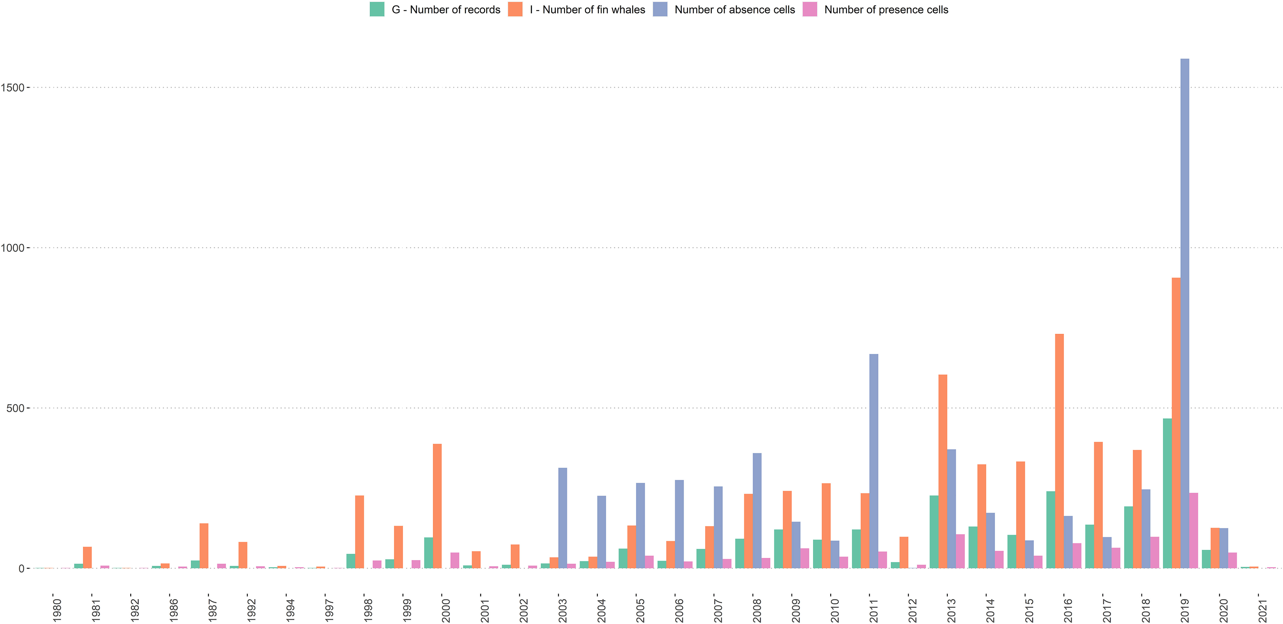
Figure 1 Number of fin whale groups (G; green bars); individuals (I; orange bars), Number of absence cells (C_absence; blue bars); Number of presence cells (C_presence; pink bars) per year.

FIGURE 2

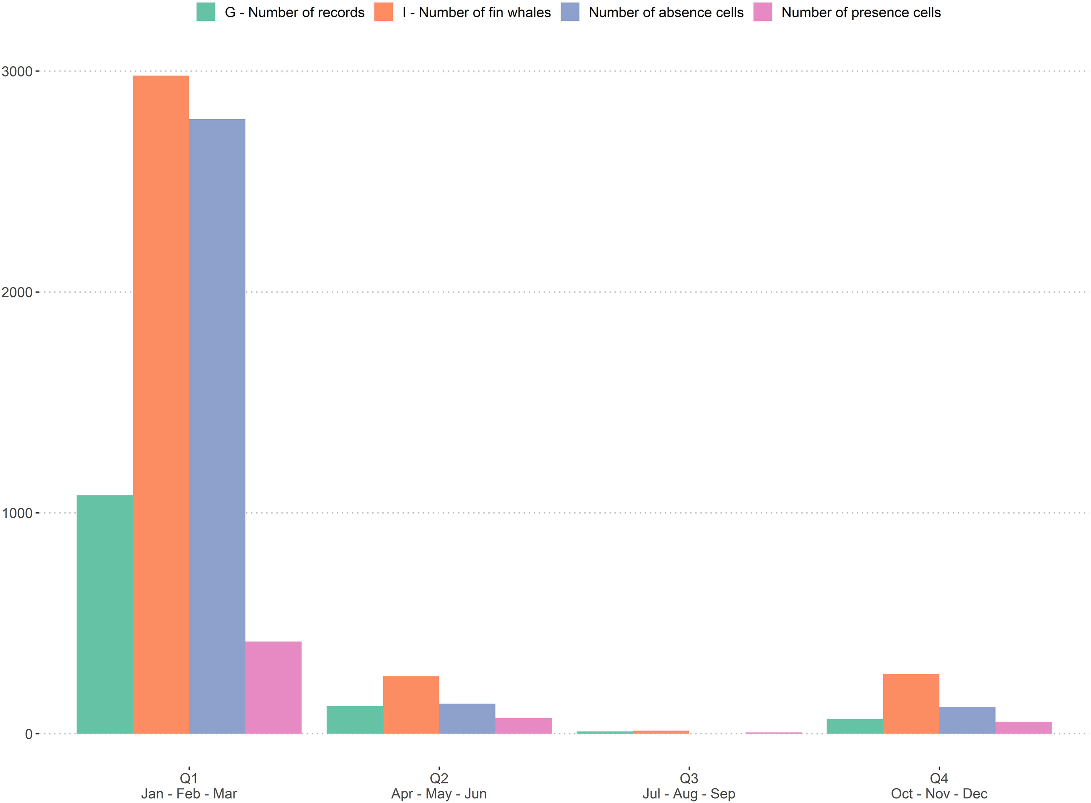
Figure 2 Number of fin whale groups (G; green bars); individuals (I; orange bars), Number of absence cells (C_absence; blue bars); Number of presence cells (C_presence; pink bars) per quarter. Q1: Jan – Mar; Q2: Apr – Jun; Q3: Jul – Sep; Q4: Oct – Dec.

FIGURE 3

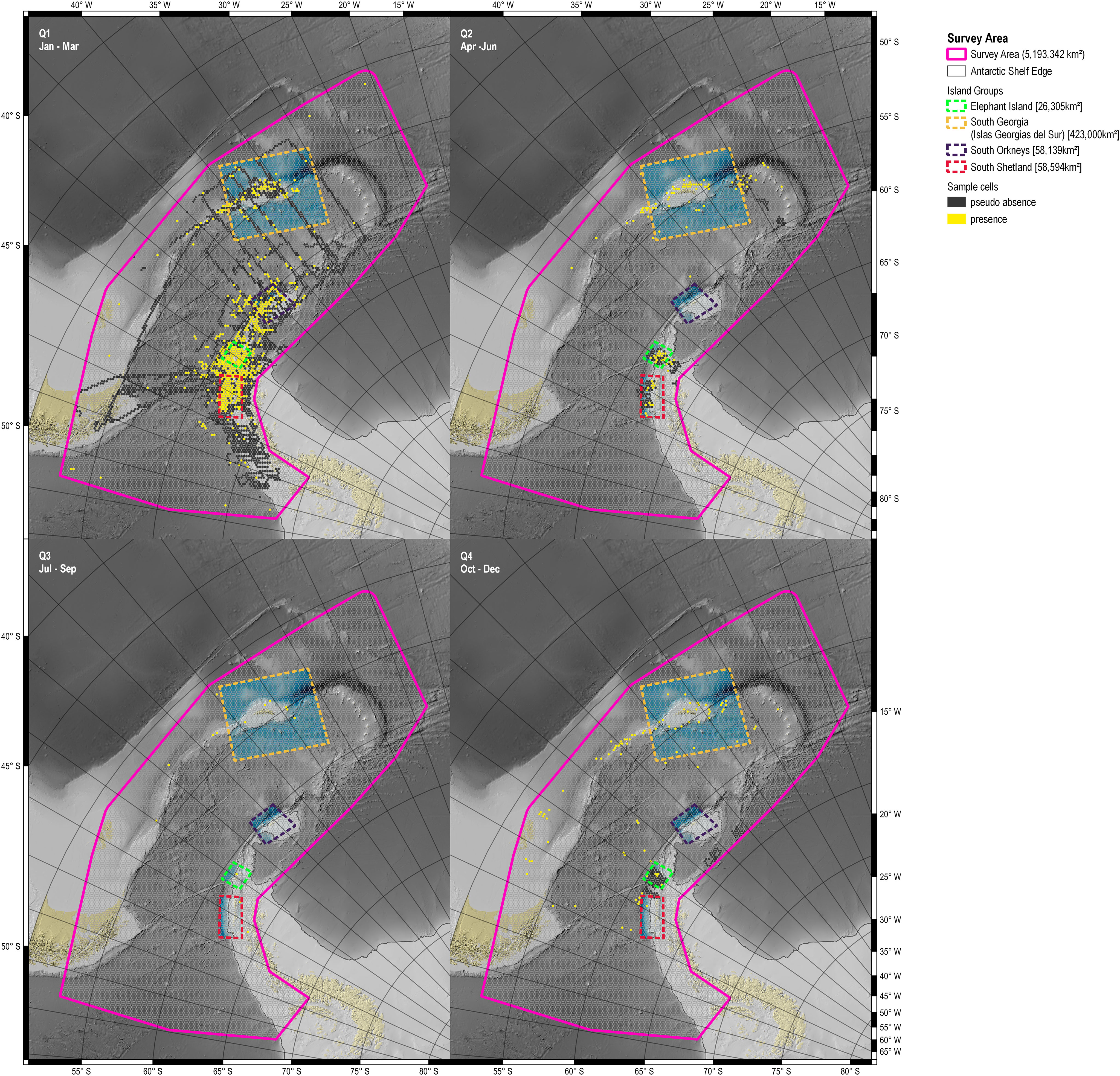
Figure 3 Sample grid as used in the SDM and RFGLS modelling step. Yellow cells: cells with confirmed presence of fin whales; black cells: cells with pseudo absence; transparent cells: cells not covered by data in the respective quarter. Background bathymetry based on IBCSO v2 (Dorschel et al., 2022). Q1: Jan – Mar, Q2: Apr – Jun, Q3: Jul-Sep; Q4: Oct – Dec.

Presences were recorded in 1,193 sample grid cells and pseudo absences in 5,445 cells (Table 3). Absences were not available for data before 2003. The distribution of data revealed consistent coverage gaps, as most records available for this analysis were collected along established travel routes and popular destinations for either scientific Antarctic expeditions or touristic ventures (e.g. South Georgia (Islas Georgias del Sur), Elephant Island). As a result, data coverage concentrated in certain localities (i.e. the island groups) and was biased towards the austral summer months January-March. The spatial distribution of sighting records showed a strong positive bias towards South Georgia (Islas Georgias del Sur) and the Antarctic Peninsula (Figure 3).

TABLE 3

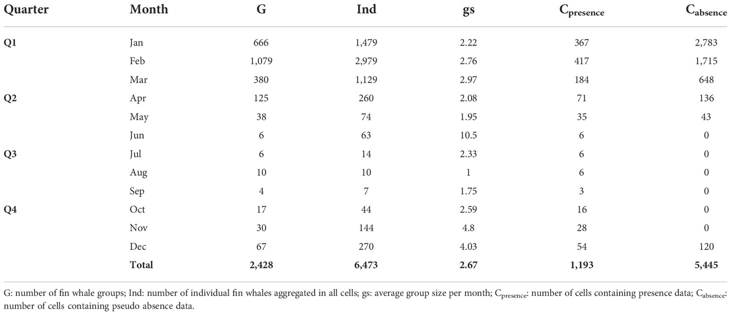
Table 3 Summary of records and number of sighted individuals and across months, aggregated on sample grid cells.

3.2. Species distribution model

We tested 20 models with different covariate combinations for each quarter using the covariates available for each quarter (Table 4; Figures S3–S5).

TABLE 4

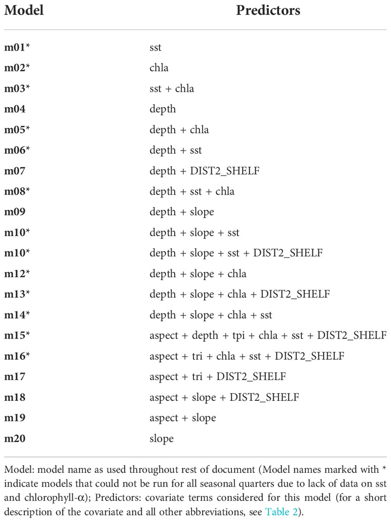
Table 4 Model definition for the SDM model of fin whale presence/pseudo absence records.

We used AUC and Cohen’s Kappa for model selection (Figures 4, 5; Tables S2, S3). The high overall number and good coverage in Q1 (Jan – Mar) was reflected in consistent ROC AUC values around 0.7, whereas the widest range in AUC values were found for models for the spring quarter Q4 (Oct – Dec). For quarter Q2 (Apr – Jun), the exclusion of sst and chla led to few remaining model runs for that season. Similarly, Cohen’s Kappa followed a similar trend, with high values in Q1 and a wide range in Q4. Data sparsity (presence cells n= 15, Table 3) led us to remove quarter Q3 from all subsequent analysis.

FIGURE 4

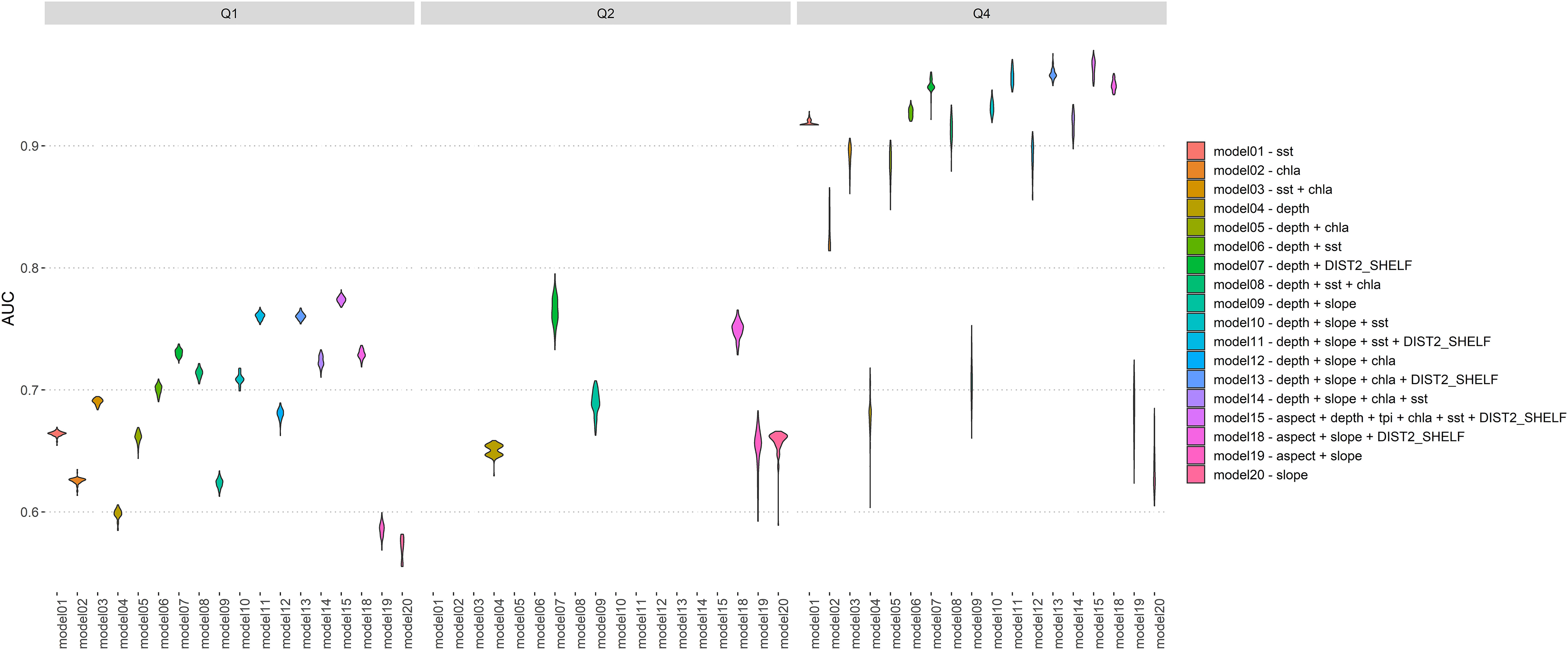
Figure 4 Summary of AUC (area under curve) for all maxent models in quarters Q1 (Jan-Mar), Q2 (Apr -Jun) and Q4 (Oct – Dec). Violins based on kernel density of 100 replicate AUC values.

FIGURE 5

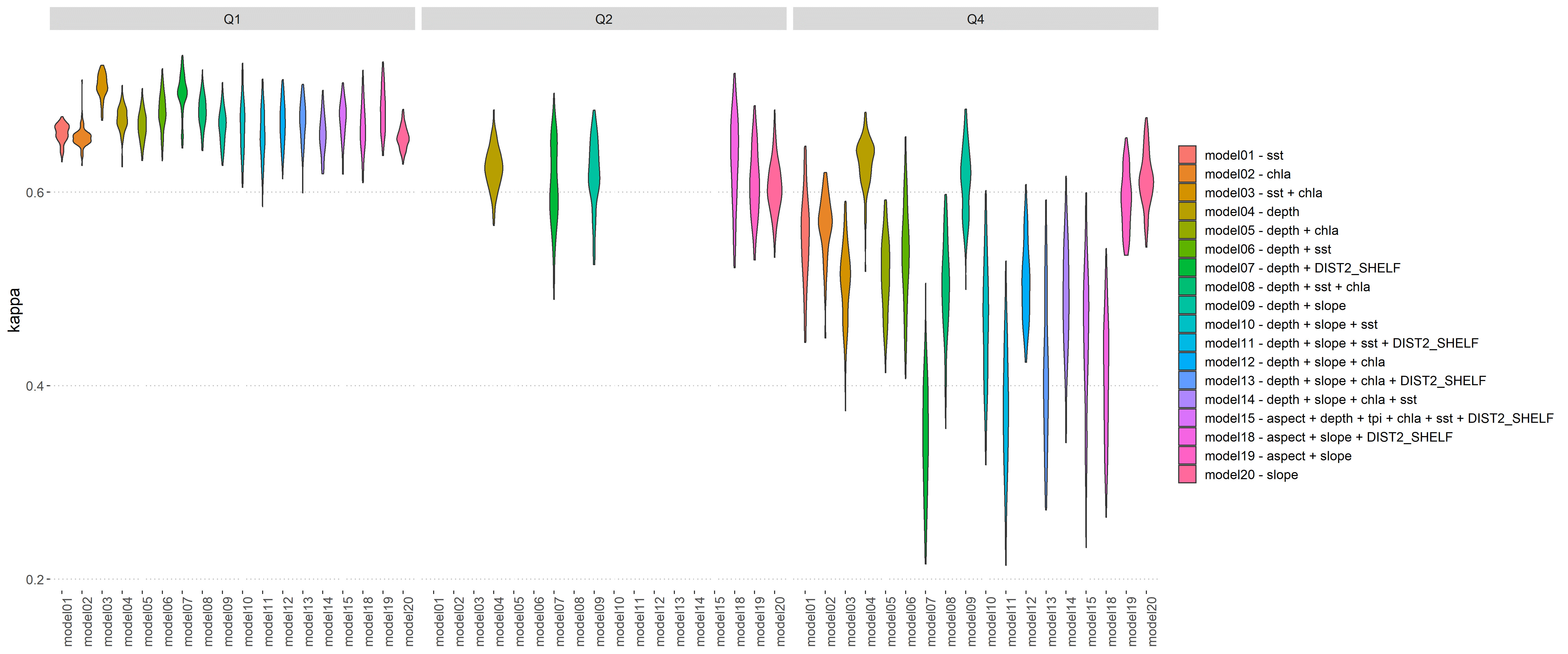
Figure 5 Summary of Cohen’s kappa for all maxent models in quarters Q1 (Jan-Mar), Q2 (Apr -Jun) and Q4 (Oct – Dec). Violins based on kernel density of 100 replicate Cohen’s kappa.

The best model for each quarter is given in Table 5 (diagnostics are shown in supplement Table S4 and Figures S6–S8, S12).

TABLE 5

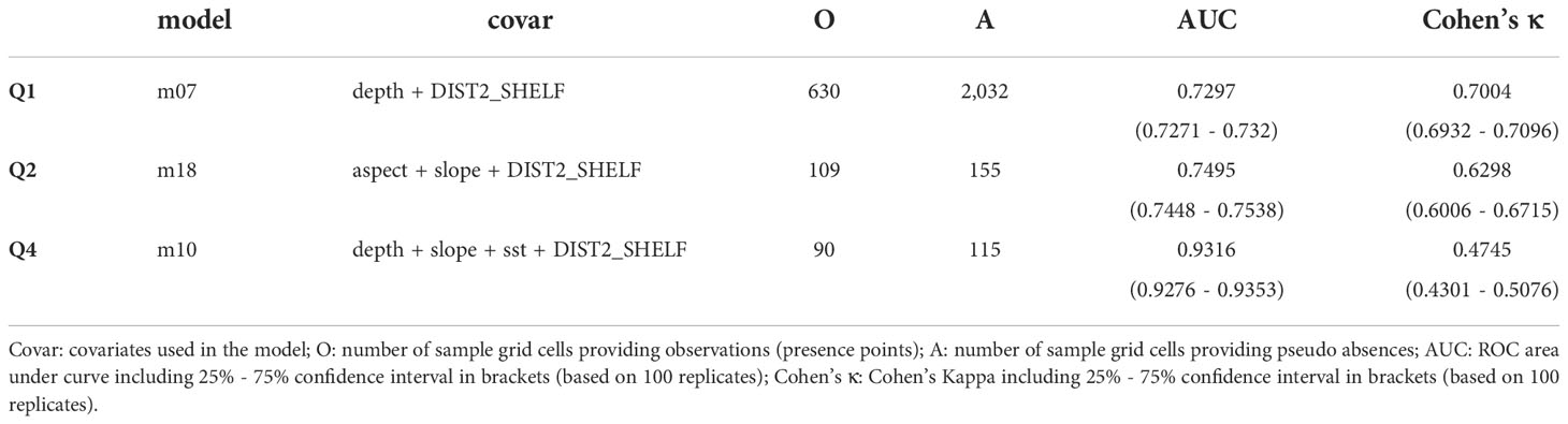
Table 5 Model parameters for the selected maxent models.

Using the selected models (Table 5), we predicted the probability of SHFW presence (p_presence) for each seasonal quarter (Figure 6) and the threshold mask based on the combined sensitivity (true positive rate) and specificity (true negative rate) (Figure 7). In Q1 (Jan - Mar), high SHFW presences were predicted on the shelf along the Antarctic Peninsula. In Q2 (Apr - Jun), no apparent pattern could be observed. For Q4 (Oct - Dec), we predicted highest probabilities of SHFW presence further offshore, beyond the shelf.

FIGURE 6

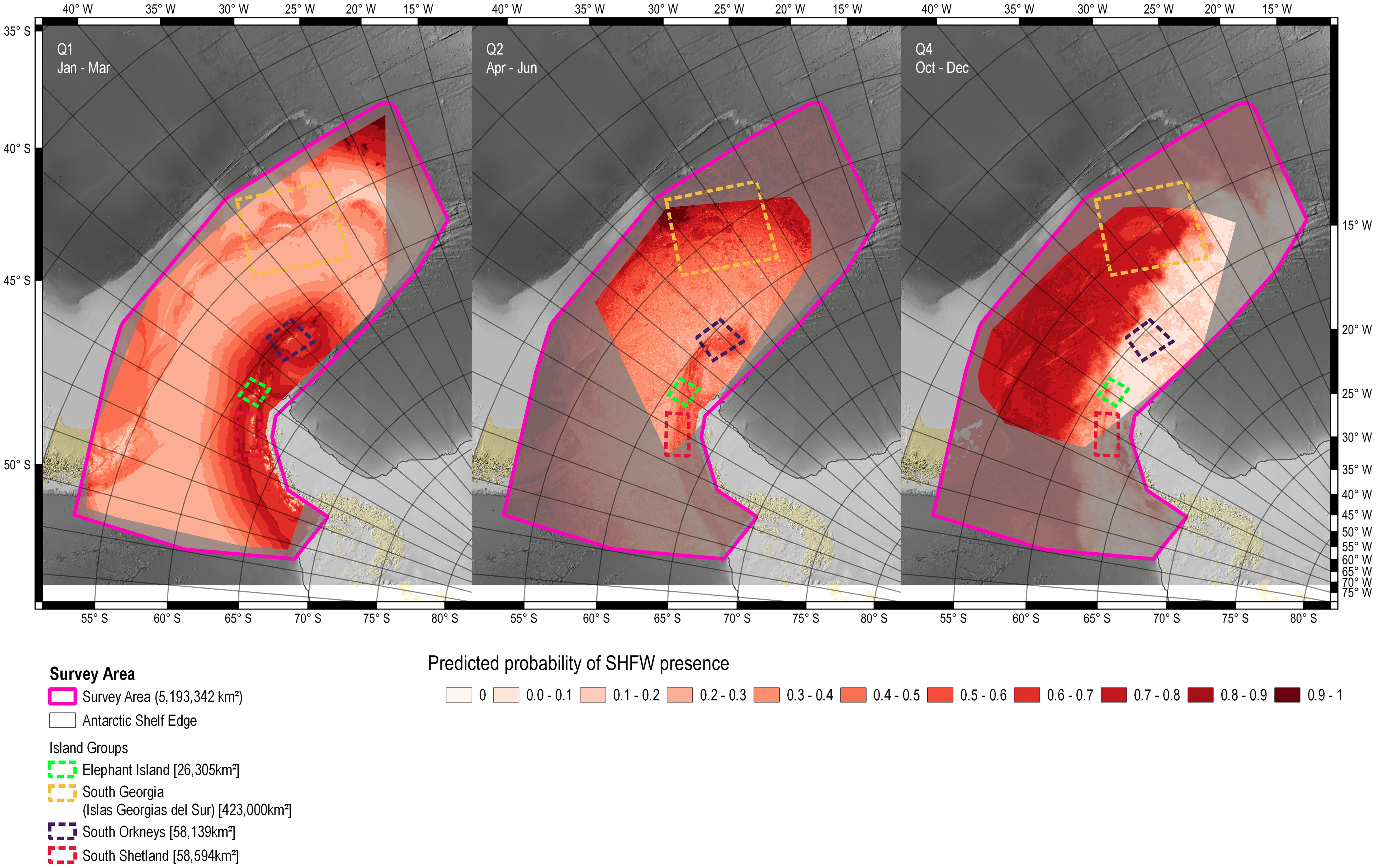
Figure 6 Predicted probability of fin whale presence per seasonal quarter (p_presence). Parts of the study area that did not provide presence records for a given seasonal quarter are dimmed. Quarter Q3 (July – September) was excluded due to lack of data. Q1: Jan – Mar, Q2: Apr – Jun, Q4: Oct – Dec.

FIGURE 7

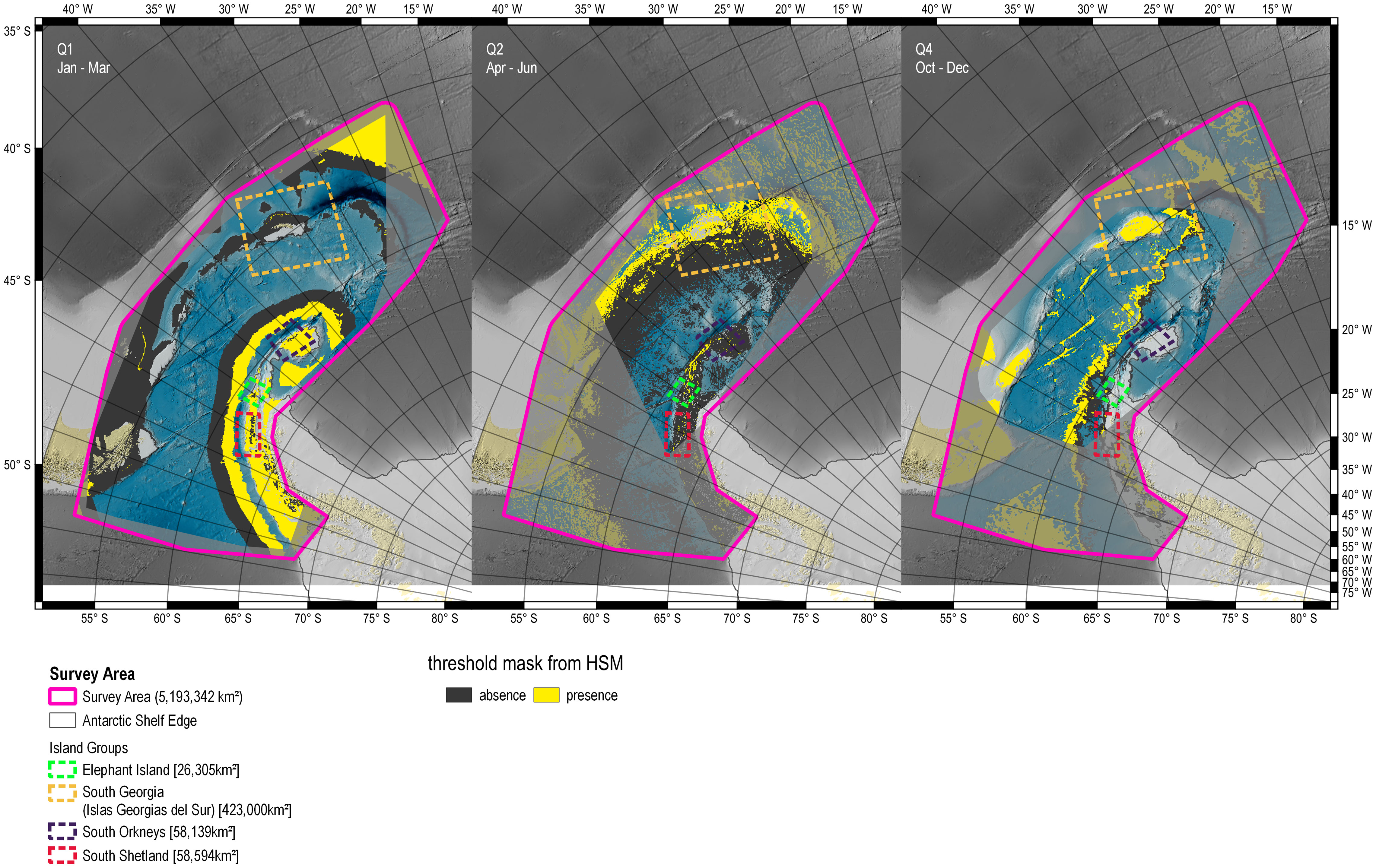
Figure 7 Predicted presence/absence of SHFW presence per seasonal quarter (p_threshold). Parts of the study area that did not provide presence records for a given seasonal quarter are dimmed. Quarter Q3 (July – September) was excluded due to lack of data. Q1: Jan – Mar, Q2: Apr – Jun, Q4: Oct – Dec.

3.3. Local abundance estimastion (RF-GLS)

The sample grid for Q1 provided the highest number of input cells for the RF-GLS. Predictive model accuracy was highest for Q4, with a median accuracy of 0.6332 (95% CI: 0.3426 - 0.9916), followed by Q1 with 0.5834 (95% CI: 0.2767 - 1.2015) and Q2 with 0.535 (95% CI: 0.3186 - 0.8789). The widest margin for p_accuracy was observed for model predictions in Q1, with an interquartile range of 0.9247 compared to Q2 (0.6490) and Q4 (0.5603; Table 6; Figures S9–S11).

TABLE 6

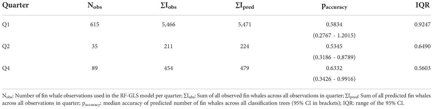
Table 6 Diagnostics for the RF-GLS model using the set of input data as test set.

In Q1, the RF-GLS predicted very high numbers of fin whales throughout the sub areas of Elephant Island, the South Orkney and the South Shetland Islands. In the sub area of South Georgia (Islas Georgias del Sur) a heterogeneous distribution pattern was predicted. In Q2, fewer animals were predicted in the three sub areas of Elephant Island, the South Orkney and the South Shetland Islands, still with local highs in abundances, albeit more dispersed than in the other quarters. South Georgia (Islas Georgias del Sur) showed a heterogeneous distribution, with the higher numbers of predicted fin whales close to the shoreline in Q1 and Q2 and a more dispersed distribution of high abundance cells in Q4 seemingly further away from the shelf. Q4 shows a distinct increase in numbers around Elephant Island and South Georgia (Islas Georgias del Sur) and low numbers in the other two sub areas (Figure 8).

FIGURE 8

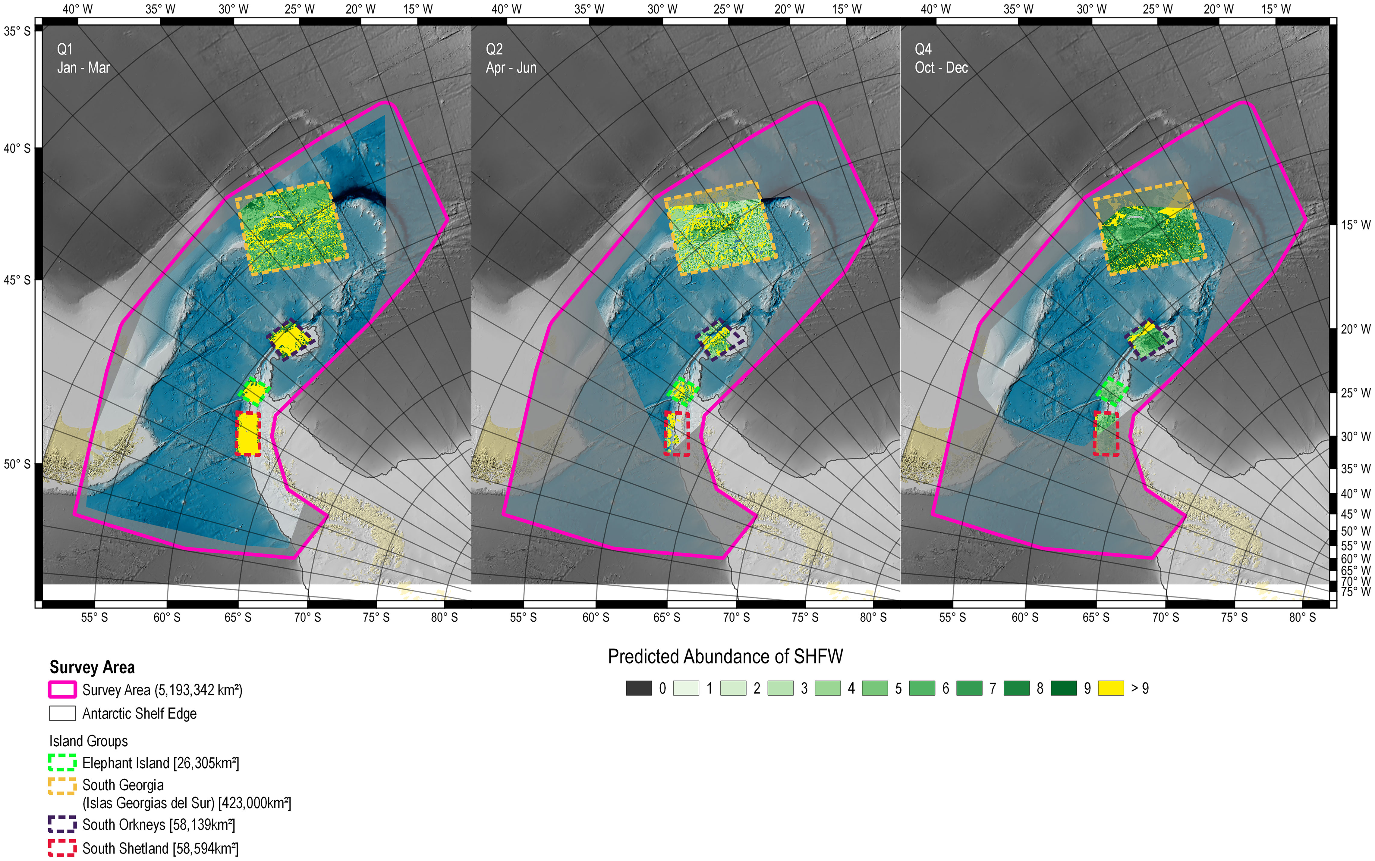
Figure 8 Number of fin whales per cell and seasonal quarter as predicted by the RF-GLS mode (N_RFGLS). Parts of the study area that did not provide presence records for a given seasonal quarter are dimmed. Quarter Q3 (July – September) was excluded due to lack of data. Q1: Jan – Mar, Q2: Apr – Jun, Q4: Oct – Dec.

3.4. Combination of SDM and RF-GLS

We multiplied the binary threshold mask from the SDM threshold (Figure 7) with the RF-GLS results (Figure 8) in order to mask the predicted abundances by the presence absence prediction from the SDM (Figure 9). Low probabilities for p_presence from the SDM set areas for which fin whales were predicted by the RF-GLS to zero. Predicted abundances in Q1 (Jan – Mar) were moderately high in the three sub areas of Elephant Island, the South Orkney Islands and the South Shetland Islands. Almost no fin whales remained within the sub area of South Georgia (Islas Georgias del Sur) after masking for presence. Distinct small areas of higher concentration of fin whale numbers were predicted within the sub area of the South Orkney Islands and Elephant Island in Q2. In the sub area of South Geogia (Islas Georgias del Sur), a heterogeneous distribution with no visible centre of concentration was observed in Q2. In Q4 (Oct – Dec) a centre of concentration of high fin whale numbers was predicted in the sub area of South Georgia (Islas Georgias del Sur). Few SHFW were predicted in the other three sub areas. Abundance and density estimates for all sub areas are shown in Table 7.

FIGURE 9

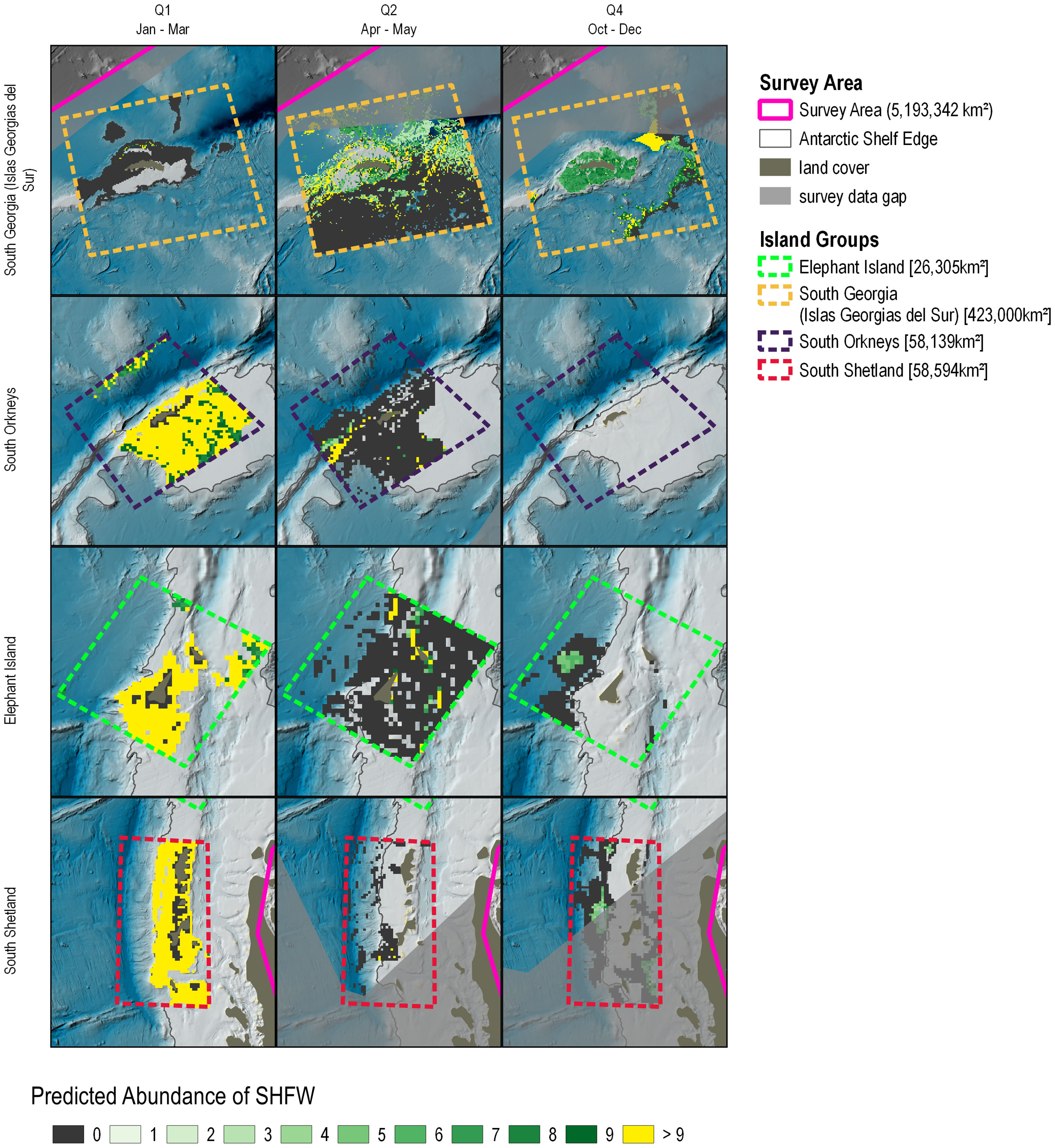
Figure 9 Number of fin whales per cell and seasonal quarter (N_adj) based on combined results from the SDM and RF-GLS. From top to bottom: South Georgia (Islas Georgias del Sur), South Orkney Islands, Elephant Island, South Shetland Islands. Parts of the study area that did not provide presence records for a given seasonal quarter are dimmed. Quarter Q3 (July – September) was excluded due to lack of data. Q1: Jan – Mar, Q2: Apr – Jun, Q4: Oct – Dec.

TABLE 7

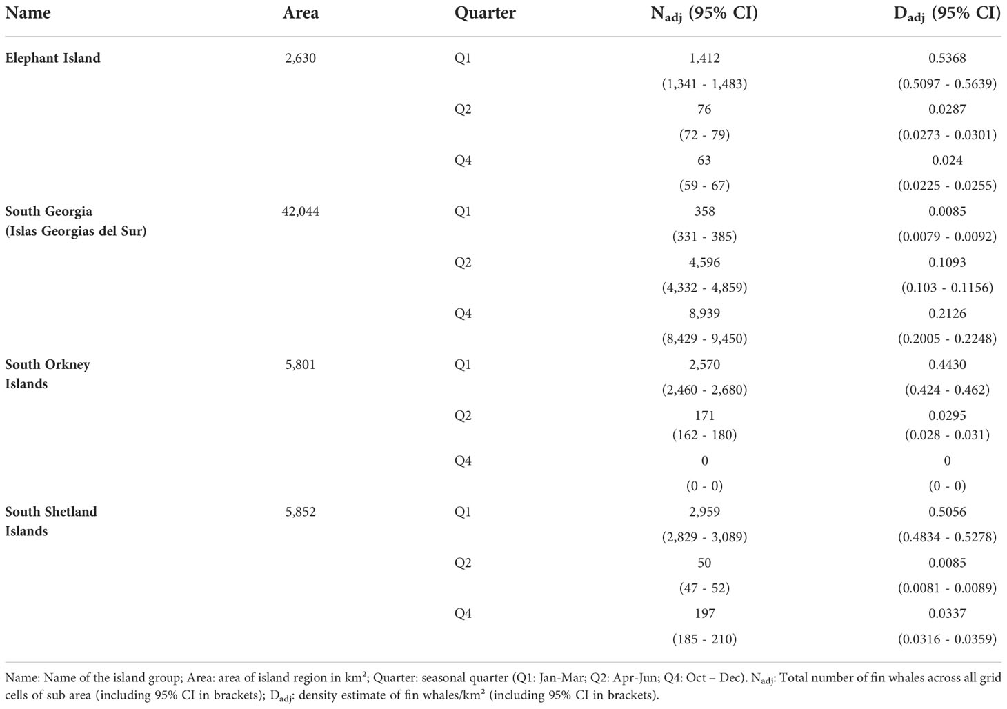
Table 7 Summary for each sub area.

The highest density across all quarters and island groups was predicted for Elephant Island in Q1 (0.5366 ind./km²) followed by the South Shetland Islands in Q1 (0.5054 ind./km²). South Georgia (Islas Georgias del Sur) showed a slight increase of densities between quarters Q1 to Q4. In some areas, our abundance model predicted no SHFW due to low estimates of p_presence (and therefore a p_threshold of zero within these areas).

4. Discussion

Fin whales are one of the most understudied baleen whales, yet were the most heavily hunted in the Southern Hemisphere (Rocha et al., 2015), and are now being seen in high densities at high latitudes again (Herr et al., 2022). Historically, the Scotia Arc was at the epicentre of commercial whaling, with fin whales particularly heavily hunted (Leaper and Miller, 2011; Calderan et al., 2020; Jackson et al., 2020), highlighting the historical importance of the region for this species.

The data compiled for this analysis represents the most comprehensive set of fin whale sighting records from the Scotia Arc to date, and provides the first overview of fin whale distribution in the area since the CCAMLR and IDCR/SOWER surveys in the early 2000s (Branch and Butterworth, 2001; Reilly et al., 2004). Using our approach of combining an ensemble learning model with the results of a maximum entropy model, we were able to update this estimate based on more recent opportunistic data. The 2000 CCAMLR survey estimated summer fin whale abundance across the Scotia Sea and Antarctic Peninsula at 4,672 [CV 42.37, (Reilly et al., 2004)]; our summer abundance estimates combined are over 1.5x this estimate; these new data are opportunistic and do not include all areas in the Scotia Arc, but still point to an increase in overall abundance of fin whales across the Scotia Sea and Antarctic Peninsula region.

This study proposes a new method to use opportunistic sighting records (if associated with critical information, i.e. species identification, group size, geographic position and the sighting date) as a data source for information on distribution and orders of magnitude of abundance.

4.1. Seasonal and regional distribution of SHFW

Our modelling suggests the highest fin whale presence changes offshore of the islands and away from the shelf break between October and December to closer to the Antarctic Peninsula from January to March. In Q4 (October-December) predictions show highest probabilities of fin whale presence off the islands and further away from the shelf break. In Q1 (January-March), the observed distribution shifts closer to the Antarctic Peninsula and concentrates around the Islands along the Peninsula. In Q2 (April-June) the distribution is more dispersed with no clear pattern of concentration. We hypothesise that these patterns may at least partly be explained by migratory movements to and from known feeding areas along the Antarctic Peninsula (Kemp and Bennett, 1932), with fin whales migrating from lower latitudes at the onset of austral spring (October), reaching the feeding grounds in austral summer (January-March), starting to leave them again in autumn (April) and rarely seen in winter. This is further supported by the covariates selected in the models. Sea surface temperature was a good predictor during Q4 (October-December) when fin whales are likely migrating into the area. In the quarters Q1 and Q2, bathymetry was the main driver for the modelled distribution, although it has to be noted that for Q2, SST and CHLA were not available. Q1 showed a positive correlation of presence probabilities with proximity to the shelf break, when fin whales are feeding at their presumed feeding grounds (Herr et al., 2022). For winter (late Q2 and Q3), data coverage in this study was too low to shed any light on the effects of migratory timing on fin whale distribution. The scarcity of sightings in austral autumn and winter must partly be attributed to lower effort, since most scientific and tourist expeditions collect data during the austral spring and summer months. Limited daylight hours additionally reduce sighting effort considerably during autumn and winter months. However, acoustic recording show a steep decrease in fin whale calling activity around Elephant Island from July/August onwards (Širović et al., 2004; Širović et al., 2009; Burkhardt et al., 2021), suggesting a withdrawal of fin whales from that area.

The observed distribution of fin whales from the SDM also reflects historic observations from this region. Whalers of the 20^th century described a peak in whale sightings in Antarctic waters from January to March, and lowest numbers in July and August (Mackintosh et al., 1966). Whaling for fin whales was carried out around South Georgia (Islas Georgias del Sur) from September to May, with most catches taken between December and February, peaking in January. Around the South Shetland Islands, whaling for fin whales was carried out from December (rarely November) to April with high catch numbers from January to April, peaking in March (Kemp and Bennett, 1932). Catch rates and distribution of whaling effort likely reflect abundance (de la Mare, 2014), but at the same time coincide with best weather and daylight conditions for spotting and hunting whales. Therefore, using historic whaling records as proxy for historic abundance and distribution are likely biased by effort to a certain degree.

4.2. Local abundance estimates

Comparison of the adjusted abundance estimates from the combined SDM and RF-GLS in the sub areas with published estimates from local surveys indicate that our estimates for Elephant Island, the South Shetlands and the South Orkneys are consistent with estimates from dedicated surveys. In January-March 2013, high fin whale densities were predicted in an area encompassing Elephant Island, and the South Shetland Islands [DP - Drake Passage in (Herr et al., 2016)]. Densities of fin whales were estimated at 0.117 (95% CI: 0.053–0.181) fin whales/km² and a total of 4,898 (95% CI 2,221 - 7,575) fin whales/km². In February-March 2016, minimum average densities of fin whales were estimated at 0.0268 ± 0.0183 fin whales/km² in a 19,750 km² area around Elephant Island and a minimum density of 0.0588 ± 0.0381 fin whales/km² in a 13,550 km² area around the South Orkney Islands (Viquerat and Herr, 2017). For March-April 2018, (Herr et al., 2022) report 0.1688 (95% CI: 0.0922 – 0.3498) fin whales/km², corresponding to 3,436 (1876 – 7,130) individuals within a 20,375 km² area divided across three distinct hotspots around Elephant Island and the South Shetland Islands. These density and abundance estimates are lower than our predictions of 0.5368 (Elephant Island), 0.4430 (South Orkney Islands) and 0.503 (South Shetland Islands) fin whales/km² in the summer (Q1) period.

However, the abundance estimates presented here must be treated with caution. Compared to results from a conventional survey design, our abundances are associated with very narrow confidence intervals that represent the noise around the expected means of the model parameters rather than the difference between observed and predicted fin whale numbers. Furthermore, our results are likely biased by data availability. For example, an abundance estimate of zero (as seen in Q4 for the South Orkney Islands) is highly unlikely. While this bias in data availability is a strong argument to focus on the results of Q1 (January-March), results for seasons Q2 and Q4 seem well within the range that we would consider reasonable for most of the investigated island groups. If some of these areas serve as feeding areas, migratory guideposts or resting spaces, we do not expect animals to be evenly distributed, but instead in local clusters as predicted here and observed in other studies (Joiris and Dochy, 2013; Burkhardt et al., 2021; Herr et al., 2022). Based on a recent snapshot survey, (Herr et al., 2022) predicted a clustered distribution of fin whales in Q1, that likely coincides with the distribution of available prey (Santora et al., 2010; Santora et al., 2014; Herr et al., 2016). This observation might explain the high densities we report for our sites, which are considerably smaller in scale and might therefore not include the steep falloff in abundance observed in (Herr et al., 2022); these areas of lower abundances were probably included in the area estimates from 2013 and 2016 (Herr et al., 2016; Viquerat and Herr, 2017). Considering that the abundances reported here are not traditional estimates based on snapshot surveys, they are not suited to base concrete management actions on, like the determination of potential biological removal. We consider the true abundance of the three areas combined to fall somewhere between the estimates for Q1. This is further emphasised by the fact that fin whales seem to be ubiquitous along the Western Antarctic Peninsula as predicted by the SDM. This result is likely biased by the high frequency of visits from scientific and touristic cruises, leading to an inflated p_presence in these areas throughout the summer (Q1). For the remaining seasons, there are few studies that allow comparisons to our estimates.

4.3. Method discussion

The combination of species distribution models and machine learning methods is an emerging field in ecology [e.g. (Effrosynidis et al., 2020; Beery et al., 2021)]. In our study, the combination of SDM and a random forest ensemble learning algorithm enabled us to derive information on abundance from a multi-source heterogeneous data set of mainly opportunistic sighting records and to present an additional set of abundance estimates for some of the most frequently visited research areas in the Southern Ocean. While abundance estimates from opportunistic sighting data that include at least some information on search effort have been explored before (Ver Hoef et al., 2021), presence-only (or presence-absence) data that do not contain any information on search effort have not been used to quantify abundances yet. By combining results from both methods based on the same data set, we were able to produce rough estimates of abundance that align with dedicated surveys in select regions and seasons. For populations for which comprehensive survey data are not available, this method may provide the only means to obtain information on abundance. Without the prerequisites for a dedicated distance sampling survey, considering the observed group sizes a spatial stochastic process is a good approximation for uncorrected group size abundances across an area covered by opportunistic sightings. However, the lack of information on search effort prevents reasonable correction for pseudo absences, which is further complicated by the lack of information on the availability bias of each sighting record. Ensemble learning models offer an unsupervised method to model data ‘as is’, i.e. hypothesis free and based on bootstrapped permutations of the observed data. Model selection is an internal feature of ensemble learning approaches, in which the ensemble group (in our case the group of 1,000 individual trees each seeded with random covariate combinations along their nodes) is tasked with finding the optimal solution for one observation by finding the best solution for all observations by numerical optimisation. In our case, it was not possible to compare different random forest models with each other, as all would converge to similar results (limited by the variation of our input data permutations). We therefore considered our RFGLS estimates as valid and optimal solutions to our input data, which was confirmed by the predictive capability for all quarters. We did not include absences in the RFGLS, since our data were zero inflated due to the large number of absences compared to presences. We were able to mitigate the lack of predicted zeroes in the RFGLS by combining its predictions with the threshold of fin whale presence derived from the SDM. In our setup, we used a threshold to limit the prediction of fin whale presence from the SDM to the information conveyed by our observed data. A threshold sensitivity of 90% and the combined sensitivity criterion (true positive rate) and specificity (true negative rate) (Liu et al., 2011; Liu et al., 2013) can be considered very strict, as it is purely based on the covariate space that was covered by the respective observed data. This also explains the narrow confidence bands for the abundance estimates, since they were mostly driven by the results of the maxent modelling (and hence are based on 100 replicates of models containing mostly static covars and thus little uncertainty). As such, these should be treated as uncertainties of the posterior distribution of abundances and not be used to run comparison metrics with other abundance estimates.

We therefore consider our threshold masks very conservative estimates of fin whale presence. If we consider that we are also dealing with a very conservative estimate of presence versus pseudo absences, our results are underestimates rather than overestimates of the true number. Using the observed data in larger spatial bins simplified the estimation of the spatial neighbourhood structure in the SDM and RFGLS approach, while predicting on the regular 5 km stack of covariates enabled fine scale implementation of said spatial effects in the results.

4.4. Data gaps and limitations

The limited accessibility of the study area due to adverse conditions during certain periods of the year is reflected in the data availability of the two environmental covariates (chlorophyll-α and SST) used in this study. Cloud cover, daylight times and ice extent during the austral winter severely impacted chlorophyll-α and sea surface temperature data availability for Q2 and Q3, leading to gaps in the prediction for given months. In addition, satellite borne data for SST and chlorophyll- α was not available at a sufficient spatial resolution for the years prior to 2002. While most of our data was collected after 2000, some records had to be assigned averaged SST and chlorophyll-α from subsequent years. This was particularly relevant for the area around South Georgia (Islas Georgias del Sur), where regular observation data since 1978 (the cut-off year for this study) was provided by the South Georgia Heritage Trust. Increased data collection in the central and eastern Scotia Arc, areas further offshore from the western Antarctic Peninsula, and the Drake Passage would improve confidence in fin whale distribution in those areas currently characterised by significant data gaps, especially during months with less data (e.g. June to November). Given the difficulty of executing a dedicated survey for cetaceans in these remote areas, advances in monitoring whale populations such as remote sensing data may help with some of these data gaps, although there are still challenges in distinguishing between species in areas with mixed species aggregations (Fretwell et al., 2014; Cubaynes et al., 2018; Borowicz et al., 2019; Bamford et al., 2020; Höschle et al., 2021).

Data availability statement

The original contributions presented in the study are publicly available. This data can be found here: https://github.com/sviquerat/SoHemFinWhales.

Ethics statement

Ethical review and approval was not required for the animal study because there was no interaction with live animals in this study.

Author contributions

SV and HH conceived and designed the study and wrote the original draft manuscript. HH acquired funding for the project. SV analyzed the data. All authors contributed to the article and approved the submitted version.

Funding

This joint data analysis was funded by the Southern Ocean Research Partnership of the International Whaling Commission (IWC-SORP) within the project Recovery status and ecology of Southern Hemisphere fin whales (Balaenoptera physalus). This work was supported by the German Research Foundation (DFG) in the framework of the priority program ‘Antarctic Research with comparative investigations in Arctic ice areas’, SPP1158, grant HE 5696/3-1. Work by Fundación Cethus was funded by IWC-SORP, Whale and Dolphin Conservation and Fondation Prince Albert II de Monaco. Work by projects Baleias and Interbiota of the Brazilian Antarctic Programme was funded by the National Council for Scientific and Technological Development (CNPq) under the Ministry of Science, Technology, and Innovations (MCTI). British Antarctic Survey (BAS) expeditions were funded by DARWIN grant DPLUS057, EU BEST 2.0 Medium Grant 1594, WWF UK, South Georgia (Islas Georgias del Sur) Heritage Trust, the Friends of South Georgia Island (Islas Georgias del Sur) and the UK Foreign and Commonwealth Office. These studies form part of the Ecosystems component of the British Antarctic Survey Polar Science for Planet Earth Programme, funded by The Natural Environment Research Council. The contributed sighting data of fin whales from the IMR/BAS survey was supported by the Institute of Marine Research (IMR) in Norway and the Norwegian Ministry of Trade, Industry and Fisheries (NFD, via project number 15208). The BAS-UK contribution was supported by the UK Research and Innovation - Natural Environment Research Council and Polar Regions Department, UK Government. Additional support was provided by the Association of Responsible Krill Harvesting Companies (ARK; www.ark-krill.org), and Aker Biomarine AS.

Acknowledgments

Our thanks go to the Instituto Antártico Argentino, Dirección Nacional del Antártico, Ministerio de Relaciones Exteriores y Culto (Argentina), Prefectura Naval Argentina and the Comissão Interministerial para os Recursos do Mar (CIRM)-Brazilian Navy. We would like to thank Ted Cheeseman and happywhale.org, the South Georgia Heritage Trust and the South Sandwich Islands (Islas Sandwich del Sur) for their data contributions. Special thanks for data collection go to M. V. Reyes Reyes, A. Marino and M. Iñíguez Bessega from Cethus, all volunteers at South Georgia (Islas Georgias del Sur) Museum for compiling sightings data and Sarah Lurcock and Marie Shafi of South Georgia Heritage Trust. We thank the officers, crew, and scientific personnel of all expeditions and vessels that collected data: RV Kronprins Haakon, FF Cabo de Hornos, RRS Discovery, SB 15 Tango, GC 28 Prefecto Derbes, GC 189 Prefecto García and ARA Almirante Irizar, RV Polarstern, PV Almirante Maximiano and NApOc Ary Rongel. Satellite borne chlorophyll-α and sea surface temperature was created by NASA Goddard Space Flight Center (Ocean Ecology Laboratory, Ocean Biology Processing Group) using the Sea-viewing Wide Field-of-view Sensor (SeaWiFS) Ocean Color Data. Data was downloaded on 2019/02/29.

Conflict of interest

The authors declare that the research was conducted in the absence of any commercial or financial relationships that could be construed as a potential conflict of interest.

Publisher’s note

All claims expressed in this article are solely those of the authors and do not necessarily represent those of their affiliated organizations, or those of the publisher, the editors and the reviewers. Any product that may be evaluated in this article, or claim that may be made by its manufacturer, is not guaranteed or endorsed by the publisher.

Supplementary material

The Supplementary Material for this article can be found online at: https://www.frontiersin.org/articles/10.3389/fmars.2022.1040512/full#supplementary-material

References

Archer F. I., Brownell R. L., Hancock-Hanser B. L., Morin P. A., Robertson K. M., Sherman K. K., et al. (2019). Revision of fin whale balaenoptera physalus (Linnaeus 1758) subspecies using genetics. J. Mammal. 100, 1–18. doi: 10.1093/jmammal/gyz121

CrossRef Full Text | Google Scholar

Archer F. I., Morin P. A., Hancock-Hanser B. L., Robertson K. M., Leslie M. S., Bérubé M., et al. (2013). Mitogenomic phylogenetics of fin whales (Balaenoptera physalus spp.): Genetic evidence for revision of subspecies. PloS One 8, e63396. doi: 10.1371/journal.pone.0063396

PubMed Abstract | CrossRef Full Text | Google Scholar

Bamford C. C. G., Kelly N., Dalla Rosa L., Cade D. E., Fretwell P. T., Trathan P. N., et al. (2020). A comparison of baleen whale density estimates derived from overlapping satellite imagery and a shipborne survey. Sci. Rep. 10, 12985. doi: 10.1038/s41598-020-69887-y

PubMed Abstract | CrossRef Full Text | Google Scholar

Barlow J. (2015). Inferring trackline detection probabilities, g(0), for cetaceans from apparent densities in different survey conditions. Mar. Mammal Sci. 31, 923–943. doi: 10.1111/mms.12205

CrossRef Full Text | Google Scholar

Beery S., Cole E., Parker J., Perona P., Winner K. (2021). Species distribution modeling for machine learning practitioners: A review. ACM SIGCAS Conf. Comput. Sustain. Soc 329–348. doi: 10.1145/3460112.3471966

CrossRef Full Text | Google Scholar

Borowicz A., Le H., Humphries G., Nehls G., Höschle C., Kosarev V., et al. (2019). Aerial-trained deep learning networks for surveying cetaceans from satellite imagery. PloS One 14, e0212532. doi: 10.1371/journal.pone.0212532

PubMed Abstract | CrossRef Full Text | Google Scholar

Branch T. A., Butterworth D. S. (2001). Estimates of abundance south of 60°S for cetacean species sighted frequently on the 1978/79 to 1997/98 IWC/IDCR-SOWER sighting surveys. J. Cetacean Res. Manage. 3, 251–270.

Google Scholar

Burkhardt E., Van Opzeeland I., Cisewski B., Mattmüller R., Meister M., Schall E., et al. (2021). Seasonal and diel cycles of fin whale acoustic occurrence near elephant island, Antarctica. R. Soc Open Sci. 8, 201142. doi: 10.1098/rsos.201142

PubMed Abstract | CrossRef Full Text | Google Scholar

Cabrera A. A., Hoekendijk J. P. A., Aguilar A., Barco S. G., Berrow S., Bloch D., et al. (2019). Fin whale (Balaenoptera physalus) mitogenomics: A cautionary tale of defining sub-species from mitochondrial sequence monophyly. Mol. Phylogenet. Evol. 135, 86–97. doi: 10.1016/j.ympev.2019.02.003

PubMed Abstract | CrossRef Full Text | Google Scholar

Calderan S., Black A., Branch T., Collins M., Kelly N., Leaper R., et al. (2020). South Georgia blue whales five decades after the end of whaling. Endanger. Species Res. 43, 359–373. doi: 10.3354/esr01077

CrossRef Full Text | Google Scholar

Clapham P. J., Baker C. S. (2002). “Whaling, modern,” in Encyclopedia of marine mammals. Eds. Perrin W. F., Würsig B., Thewissen J. G. M. (New York, NY: Academic Press), 1328–1332. Available at: https://linkinghub.elsevier.com/retrieve/pii/B9780123735539002832.

Google Scholar

Claro B., Pérez-Jorge S., Frey S. (2020). Seafloor geomorphic features as an alternative approach into modelling the distribution of cetaceans. Ecol. Inform. 58, 101092. doi: 10.1016/j.ecoinf.2020.101092

CrossRef Full Text | Google Scholar

Cooke J. G. (2018). Balaenoptera physalus, The IUCN Red List of Threatened Species 2018: e.T2478A50349982. doi: 10.2305/IUCN.UK.2018-2.RLTS.T2478A50349982.en. Accessed on 30 November 2022

CrossRef Full Text | Google Scholar

Cubaynes H. C., Fretwell P. T., Bamford C., Gerrish L., Jackson J. A. (2018). Whales from space: Four mysticete species described using new VHR satellite imagery. Mar. Mammal Sci. 00, 1–26. doi: 10.1111/mms.12544

CrossRef Full Text | Google Scholar

de la Mare W. K. (2014). Estimating relative abundance of whales from historical Antarctic whaling records. Can. J. Fish. Aquat. Sci. 71, 106–119. doi: 10.1139/cjfas-2013-0016

CrossRef Full Text | Google Scholar

Díaz López B., Methion S. (2019). Habitat drivers of endangered rorqual whales in a highly impacted upwelling region. Ecol. Indic. 103, 610–616. doi: 10.1016/j.ecolind.2019.04.038

CrossRef Full Text | Google Scholar

Dorschel B., Hehemann L., Viquerat S., Warnke F., Dreutter S., Tenberge Y. S., et al. (2022). The international bathymetric chart of the southern ocean version 2. Sci. Data 9, 275. doi: 10.1038/s41597-022-01366-7

PubMed Abstract | CrossRef Full Text | Google Scholar

Edwards E. F., Hall C., Moore T. J., Sheredy C., Redfern J. V. (2015). Global distribution of fin whales balaenoptera physalus in the post-whaling era, (1980-2012). Mamm. Rev. 45, 197–214. doi: 10.1111/mam.12048

CrossRef Full Text | Google Scholar

Effrosynidis D., Tsikliras A., Arampatzis A., Sylaios G. (2020). Species distribution modelling via feature engineering and machine learning for pelagic fishes in the Mediterranean Sea. Appl. Sci. 10, 8900. doi: 10.3390/app10248900

CrossRef Full Text | Google Scholar

El-Gabbas A., Van Opzeeland I., Burkhardt E., Boebel O. (2021a). Dynamic species distribution models in the marine realm: Predicting year-round habitat suitability of baleen whales in the southern ocean. Front. Mar. Sci. 8. doi: 10.3389/fmars.2021.802276

CrossRef Full Text | Google Scholar

El-Gabbas A., Van Opzeeland I., Burkhardt E., Boebel O. (2021b). Static species distribution models in the marine realm: The case of baleen whales in the southern ocean. Divers. Distrib. 27, 1536–1552. doi: 10.1111/ddi.13300

CrossRef Full Text | Google Scholar

Fretwell P. T., Staniland I. J., Forcada J. (2014). Whales from space: Counting southern right whales by satellite. PloS One 9, 1–9. doi: 10.1371/journal.pone.0088655

CrossRef Full Text | Google Scholar

Hammond P. S., Francis T. B., Heinemann D., Long K. J., Moore J. E., Punt A. E., et al. (2021). Estimating the abundance of marine mammal populations. Front. Mar. Sci. 8. doi: 10.3389/fmars.2021.735770

CrossRef Full Text | Google Scholar

Harrell J. F.E. (2018) Hmisc: Harrell miscellaneous. Available at: https://cran.r-project.org/package=Hmisc.

Google Scholar

Herr H., Kelly N., Dorschel B., Huntemann M., Kock K. H. K.-H., Lehnert L. S. L. S., et al. (2019). Aerial surveys for Antarctic minke whales (Balaenoptera bonaerensis) reveal sea ice dependent distribution patterns. Ecol. Evol. 9, 5664–5682. doi: 10.1002/ece3.5149

PubMed Abstract | CrossRef Full Text | Google Scholar

Herr H., Viquerat S., Devas F., Lees A., Wells L., Gregory B., et al. (2022). Return of large fin whale feeding aggregations to historical whaling grounds in the southern ocean. Sci. Rep. 12, 9458. doi: 10.1038/s41598-022-13798-7

PubMed Abstract | CrossRef Full Text | Google Scholar

Herr H., Viquerat S., Siegel V., Kock K.-H. H., Dorschel B., Huneke W. G. C. C., et al. (2016). Horizontal niche partitioning of humpback and fin whales around the West Antarctic peninsula: Evidence from a concurrent whale and krill survey. Polar Biol. 39, 799–818. doi: 10.1007/s00300-016-1927-9

CrossRef Full Text | Google Scholar

Hijmans R. J. (2017) Raster: Geographic data analysis and modeling. Available at: https://cran.r-project.org/package=raster.

Google Scholar

Hijmans R. J., Phillips S., Leathwick J., Elith J. (2017) Dismo: Species distribution modeling. Available at: https://cran.r-project.org/package=dismo.

Google Scholar

Ho T. K. (1995). “International Conference On Document Analysis and Recognition,” in Proceedings of 3rd international conference on document analysis and recognition (IEEE Comput. Soc. Press) iii–xx. doi: 10.1109/ICDAR.1995.601943

CrossRef Full Text | Google Scholar

Höschle C., Cubaynes H. C., Clarke P. J., Humphries G., Borowicz A. (2021). The potential of satellite imagery for surveying whales. Sensors (Switzerland) 21, 1–6. doi: 10.3390/s21030963

CrossRef Full Text | Google Scholar

Hu C., Lee Z., Franz B. (2012). Chlorophyll a algorithms for oligotrophic oceans: A novel approach based on three-band reflectance difference. J. Geophys. Res. Ocean. 117, 1–25. doi: 10.1029/2011JC007395

CrossRef Full Text | Google Scholar

IWC: International Whaling Commision (1976). Twenty-sixth report of the scientific committee (Cambridge, UK, UK). Available at: https://archive.iwc.int/?r=2093&k=47b1305db5.

Google Scholar

IWC: International Whaling Commision (1978). Twenty-eighth report of the scientific committee. SC30 (Cambridge, UK, UK). Available at: https://archive.iwc.int/?r=2093&k=ec6d82bc2d.

Google Scholar

Jackson J., Kennedy A., Moore M., Andriolo A., Bamford C., Calderan S., et al. (2020). Have whales returned to a historical hotspot of industrial whaling? the pattern of southern right whale eubalaena australis recovery at south Georgia. Endanger. Species Res. 43, 323–339. doi: 10.3354/esr01072

CrossRef Full Text | Google Scholar

Joiris C. R., Dochy O. (2013). A major autumn feeding ground for fin whales, southern fulmars and grey-headed albatrosses around the south Shetland islands, Antarctica. Polar Biol. 36, 1649–1658. doi: 10.1007/s00300-013-1383-8

CrossRef Full Text | Google Scholar

Kemp S., Bennett A. G. (1932). On the distribution and movements of whales on the south Georgia and south Shetland whaling grounds. Discovery Rep. 6, 165–190.

Google Scholar

Leaper R. R., Miller C. (2011). Management of Antarctic baleen whales amid past exploitation, current threats and complex marine eco-systems. Antarct. Sci. 23, 503–529. doi: 10.1017/s0954102011000708

CrossRef Full Text | Google Scholar

Liu C., White M., Newell G. (2011). Measuring and comparing the accuracy of species distribution models with presence-absence data. Ecography (Cop.). 34, 232–243. doi: 10.1111/j.1600-0587.2010.06354.x

CrossRef Full Text | Google Scholar

Liu C., White M., Newell G. (2013). Selecting thresholds for the prediction of species occurrence with presence-only data. J. Biogeogr. 40, 778–789. doi: 10.1111/jbi.12058

CrossRef Full Text | Google Scholar

Mackintosh N. A. (1966). “8. the distribution of southern blue and fin whales,” in Whales, dolphins, and porpoises. Ed. Norris K. S. (Berkeley and Los Angeles: University of California Press), 125–144. doi: 10.1525/9780520321373-010

CrossRef Full Text | Google Scholar

Mizroch S., Rice D. W., Breiwick J. M. (1984). The fin whale, balaenoptera physalus. Mar. Fish. Rev. 46, 20–24.

Google Scholar

Moran P. A. P. (1950). Notes on continuous stochastic phenomena. Biometrika 37, 17–23. doi: 10.1093/biomet/37.1-2.17

PubMed Abstract | CrossRef Full Text | Google Scholar

Paradis E., Blomberg S., Bolker B., Brown J., Claude J., Cuong H. S., et al. (2018) Ape: Analyses of phylogenetics and evolution. Available at: https://cran.r-project.org/package=ape.

Google Scholar

Pérez-Alvarez M. J., Kraft S., Segovia N. I., Olavarría C., Nigenda-Morales S., Urbán R. J., et al. (2021). Contrasting phylogeographic patterns among northern and southern hemisphere fin whale populations with new data from the southern pacific. Front. Mar. Sci. 8. doi: 10.3389/fmars.2021.630233

CrossRef Full Text | Google Scholar

Pérez M. J., Thomas F., Uribe F., Sepúlveda M., Flores M., Moraga R. (2006). Fin whales (Balaenoptera physalus) feeding on Euphausia mucronata in nearshore waters off north-central Chile. Aquat. Mamm. 32, 109–113. doi: 10.1578/AM.32.1.2006.109

CrossRef Full Text | Google Scholar

Phillips S. J., Dudík M., Schapire R. E. (2020) Maxent software for modeling species niches and distributions (Version 3.4.1). Available at: http://biodiversityinformatics.amnh.org/open_source/maxent/.

Google Scholar

R Core Team (2021) R: A language and environment for statistical computing. Available at: https://www.r-project.org/.

Google Scholar

Reilly S., Hedley S., Borberg J., Hewitt R., Thiele D., Watkins J., et al. (2004). Biomass and energy transfer to baleen whales in the south Atlantic sector of the southern ocean. Deep Sea Res. Part II Top. Stud. Oceanogr. 51, 1397–1409. doi: 10.1016/j.dsr2.2004.06.008

CrossRef Full Text | Google Scholar

Reisinger R. R., Friedlaender A. S., Zerbini A. N., Palacios D. M., Andrews-Goff V., Dalla Rosa L., et al. (2021). Combining regional habitat selection models for large-scale prediction: Circumpolar habitat selection of southern ocean humpback whales. Remote Sens. 13, 2074. doi: 10.3390/rs13112074

CrossRef Full Text | Google Scholar

Riley S. J., DeGloria S. D., Elliot R. (1999). A terrain ruggedness index that quantifies topographic heterogeneity. Intermt. J. Sci. 5, 23–27. doi: 10.1016/j.ecoinf.2020.101092

CrossRef Full Text | Google Scholar

Rocha R. C. J., Clapham P. J., Ivashchenko Y. V. (2015). Emptying the oceans: A summary of industrial whaling catches in the 20th century. Mar. Fish. Rev. 76, 37–48. doi: 10.7755/mfr.76.4.3

CrossRef Full Text | Google Scholar

Sagnol O., Richter C., Field L. H., Reitsma F. (2014). Spatio-temporal distribution of sperm whales (Physeter macrocephalus) off kaikoura, new Zealand, in relation to bathymetric features. New Zeal. J. Zool. 41, 234–247. doi: 10.1080/03014223.2014.936474

CrossRef Full Text | Google Scholar

Saha A., Basu S., Datta A. (2021). Random forests for spatially dependent data. J. Am. Stat. Assoc., 1–19. doi: 10.1080/01621459.2021.1950003

PubMed Abstract | CrossRef Full Text | Google Scholar

Saha A., Datta A. (2018). BRISC: Bootstrap for rapid inference on spatial covariances. Stat 7, e184. doi: 10.1002/sta4.184

CrossRef Full Text | Google Scholar

Santora J., Reiss C., Loeb V., Veit R. (2010). Spatial association between hotspots of baleen whales and demographic patterns of Antarctic krill euphausia superba suggests size-dependent predation. Mar. Ecol. Prog. Ser. 405, 255–269. doi: 10.3354/meps08513

CrossRef Full Text | Google Scholar

Santora J. A., Schroeder I. D., Loeb V. J. (2014). Spatial assessment of fin whale hotspots and their association with krill within an important Antarctic feeding and fishing ground. Mar. Biol. 161, 2293–2305. doi: 10.1007/s00227-014-2506-7

CrossRef Full Text | Google Scholar

Sepúlveda M., Pérez-Álvarez M. J., Santos-Carvallo M., Pavez G., Olavarría C., Moraga R., et al. (2018). From whaling to whale watching: Identifying fin whale critical foraging habitats off the Chilean coast. Aquat. Conserv. Mar. Freshw. Ecosyst. 28, 821–829. doi: 10.1002/aqc.2899

CrossRef Full Text | Google Scholar

Širović A., Hildebrand J. A., Wiggins S. M., McDonald M. A., Moore S. E., Thiele D. (2004). Seasonality of blue and fin whale calls and the influence of sea ice in the Western Antarctic peninsula. Deep Sea Res. Part II Top. Stud. Oceanogr. 51, 2327–2344. doi: 10.1016/j.dsr2.2004.08.005

CrossRef Full Text | Google Scholar

Širović A., Hildebrand J. A., Wiggins S. M., Thiele D. (2009). Blue and fin whale acoustic presence around Antarctica during 2003 and 2004. Mar. Mammal Sci. 25, 125–136. doi: 10.1111/j.1748-7692.2008.00239.x

CrossRef Full Text | Google Scholar

Toro F., Vilina Y. A., Capella J. J., Gibbons J. (2016). Novel coastal feeding area for eastern south pacific fin whales (Balaenoptera physalus) in mid-latitude Humboldt current waters off Chile. Aquat. Mamm. 42, 47. https://link.gale.com/apps/doc/A475126217/AONE?u=anon~53e193d0&sid=googleScholar&xid=685a9f1b. doi: 10.1578/AM.42.1.2016

CrossRef Full Text | Google Scholar

Ver Hoef J. M., Johnson D., Angliss R., Higham M. (2021). Species density models from opportunistic citizen science data. Methods Ecol. Evol. 12, 1911–1925. doi: 10.1111/2041-210X.13679

CrossRef Full Text | Google Scholar

Viquerat S., Herr H. (2017). Mid-summer abundance estimates of fin whales balaenoptera physalus around the south Orkney islands and elephant island. Endanger. Species Res. 32, 515–524. doi: 10.3354/esr00832

CrossRef Full Text | Google Scholar

Wilson M. F. J., O’Connell B., Brown B., Guinan J. C., Grehan A. J. (2007). Multiscale terrain analysis of multibeam bathymetry data for habitat mapping on the continental slope. Mar. Geod. 30, 3–35. doi: 10.1080/01490410701295962

CrossRef Full Text | Google Scholar

Wood M., Širović A. (2022). Characterization of fin whale song off the Western Antarctic peninsula. PloS One 17, e0264214. doi: 10.1371/journal.pone.0264214

PubMed Abstract | CrossRef Full Text | Google Scholar