Non-invasive estimation of coral polyp volume and surface area using optical coherence tomography

1 Introduction

Volume and surface area (SA) are important structural features of all organisms that rely on the transport and diffusion of gases and metabolites across their physical boundaries (Patterson, 1992). For tropical reef-building corals, surface area is a key parameter when quantifying ecophysiological processes (Naumann et al., 2009). For instance, rates of photosynthesis and respiration as well as photosymbiont density and pigment content are generally normalized to coral surface area (e.g., Bythell et al., 2001). However, estimates of coral surface area largely rely on indirect measures of dead coral skeleton surface area and quantification of the surface area of living coral tissue remains a major challenge, especially as corals exhibit strong plasticity in their tissue organization (Wangpraseurt et al., 2017; Laissue et al., 2020).

The most common technique used to measure coral surface area is arguably the paraffin wax dipping technique (Stimson and Kinzie, 1991), which quantifies SA from weighing bare coral skeleton coated once and twice with wax and calibrating the weight gain against a series of similar measurements on standards with known surface area. Other coating approaches use tin foil (Marsh, 1970), dye (Hoegh-Guldberg, 1988) or vaseline (Odum and Odum, 1955). More recently, 3D structured light scanning (SLS) has been used for coral surface area reconstruction and quantification (Kaandorp and Kübler, 2001; Raz-Bahat et al., 2009; Zawada et al., 2019; Koch et al., 2021). Other nondestructive methods for 3D reconstruction include photogrammetric methods such as structure-from-motion (SFM) (Pollefeys et al., 2004; Lavy et al., 2015; Lange and Perry, 2020) that create 3D locations of points on the surfaces of benthic objects. While SLS typically is limited to smaller structures and scanning of samples in air (Koch et al., 2021), SFM-based methods work with underwater photography and obtain good results on the scales of coral colonies and reef structures and with a variety of benthic organisms (Lavy et al., 2015). However, these methods do not allow for a reliable quantification of live coral tissue surface areas with microstructural features. This is because the resolution required for estimating the SA of corals that have a large contribution from small structures, such as tentacles, is not achieved. Another disadvantage of both SLS and SFM, is the requirement for surfaces to be visible from the outside, i.e., it cannot capture overhanging structures and various features that are being shaded by the morphology (Lange and Perry, 2020).

2 Here, we demonstrate the use of Optical Coherence Tomography (OCT) for non-invasive quantification at sub-mm resolution of tissue surface area and volume on living corals to resolve the morphological features of coral polyps, tentacles, and other features that substantially contribute to the surface area of live corals. OCT typically uses near-infrared radiation and determines patterns of elasticity, using directly backscattered (low coherent) photons from refractive index mismatches between tissue compartments with different microstructural features (Huang et al, 1991). The operating principle of OCT is based on interferometry using broadband low coherent light from a super luminescent diode. The incident light is split into two partially coherent beams (reference and sample beam). The sample beam penetrates the object along the z-axis, while the reference light is reflected by a retro-reflecting mirror within the imaging probe. The locally reflected light is collected and combined with the reference beam, generating a characteristic interference pattern. To generate 2D and 3D scans, galvanic mirrors move the sample beam along the x- and y-axis. OCT is well established in clinical settings and has revolutionized dermatology and ophthalmology (Drexler and Fujimoto, 2015). It allows for rapid, non-invasive tomographic imaging, and there is a plethora of literature that considers both the basic optical theory behind OCT as well as an assortment of processing techniques that are aimed at either enhancing the available information for clinical diagnosis or inferring the physical parameters of the media (Fercher et al., 2003; Drexler and Fujimoto, 2015). However, OCT was only recently introduced to coral reef science for identification of microstructural features of live corals (Wangpraseurt et al., 2017) as well as their optical properties (Spicer et al., 2019; Wangpraseurt et al., 2019). In this study, we develop a computational pipeline for OCT scans that allows for accurate and rapid characterization of live coral SA and volume with microscale resolution. We exemplify the suitability of our method using the common branching coral Pocillopora damicornis. In addition, to verify our algorithms, we calibrated our system using borosilicate spheres and ellipsoidal fish eggs, whose SA was analytically approximated from knowledge of their observed radii.

2 Methods and materials

2.1 Optical coherence tomography, theory and rationale for the algorithm

Here, we consider the goal of identifying the outside surfaces of corals that are in contact with their aqueous environment from 3-D OCT scans. Coral tissue absorption is small for NIR wavelengths commonly used in OCT (Wangpraseurt et al., 2012) and with shallow water levels above the sample, the recorded changes in reflected light are primarily a function of optical scattering (Wangpraseurt et al., 2019). Our goal in defining the outside surface of the coral is to identify the optical boundary between water and tissue. The magnitude of directly backscattered light in OCT imaging is affected by the scattering coefficient of different tissues (Spicer et al., 2019) and by the orientation of the surface relative to the incident beam. For example, a given, nearly specular, biological surface interface will yield larger reflectance when oriented perpendicular to the incident light beam than when oriented at more oblique angles (e.g., Yoo et al., 1990).

Commercial systems usually involve a range of image optimization procedures (Wagner and Horn, 2017; Wangpraseurt et al., 2017) as the primary application of such systems are clinical settings with the aim of visualizing human anatomical structures like the retina (Fercher et al., 2003). Consequently, the magnitude of the backscatter data provided by the manufacturer is not strictly proportional to the received photon flux and requires time-intensive calibration procedures (Wangpraseurt et al., 2019). The processing schemes were heretofore developed in absentia of calibrated OCT signal intensities and evaluated based on the capability of the algorithms to 1) estimate surface area in calibrated ellipsoidal targets such as borate spheres and fish eggs, and 2) to generate surfaces consistent with visual inspection of the coral specimens.

2.2 Samples and OCT imaging

Coral fragments (Pocillopora damicornis) were obtained from the Birch Aquarium (Scripps Oceanography, U.C. San Diego) and were cultivated in coral culture facilities. Corals were provided with natural seawater pumped from the Scripps Pier and maintained at a temperature of 26° C and under an 12:12 h light-dark cycle with an incident downwelling photon irradiance of 100 µmol photons m^-2 s^-1 from an aquarium lamp (Orbit Marine LED, Current, USA).

As calibration targets, we used borate spheres (~ 1 mm diameter) and fish eggs.

We used a commercially available spectral domain (SD) OCT system (Ganymede II, Thorlabs, GmbH, Dachau, Germany) with an effective focal length of 36 mm and a lens working distance of 25.1 mm (LSM03: Thorlabs, GmbH, Dachau, Germany) with a super luminescent diode emitting low coherent light centered at 930 nm. With this configuration, the system has an axial resolution of 5.8 µm and a lateral sampling resolution of 8 µm. Imaging was performed as described previously (Wangpraseurt et al., 2017; Wangpraseurt et al., 2019). Briefly, coral fragments were placed in a custom-made black acrylic flow chamber that was provided with running seawater at 26° C. Measurements were performed under low actinic light of about 80 µmol photons m^-2 s^-1 (400-700 nm) as provided by the white LED ring-light of the OCT system. The low level of irradiance was chosen to minimize coral tissue movement during imaging (Wangpraseurt et al., 2017). The relatively fast scanning of the entire coral fragment of 7.7 mm x 3.4 mm in<3 minutes also reduces the chances of movement artifacts.

2.3 Volumetric image processing

The representation of 3-D objects has a long history in computer graphics and scientific inquiry (Hughes et al, 2014). Two frequently used 3-D representations of object surfaces are that of a Voronoi tessellation and that of a polygon mesh, i.e., a collection of vertices, edges and faces that defines the shape of a polyhedral object. In both cases, the data is a set of polyhedral elements that can then be used to compute the surface area (SA) of the object by integrating the surface area of each of the polyhedral elements that are simple flat planes. Prior to defining the polyhedral elements, a 3D point cloud is established, i.e., a set of points in 3-D that lie on the surfaces or boundaries of the object. Based on this point cloud, the computation of either the meshes or the Voronoi tessellation is accomplished via a set of geometrical operations (for details, see Hughes et al, 2014). The accuracy of SA estimation is affected by surface roughness, whereas surfaces that are rougher require higher sampling. In some cases, the quasi-fractal nature of the surfaces that is especially important for rough boundaries (Kaandorp and Kübler, 2001) that can require extremely high spatial resolution to estimate the SA. In the specimens considered here, the visual appearance of the exterior of the polyps appears quite smooth. Based on this conjecture, we proceeded to compute estimates of SA from the sampled OCT data.

To compute the point cloud that defines the exterior surface of the coral from the experimentally observed 3-D matrices, several approaches can be used (Khatamian and Arabnia, 2016). The approach taken here is to compute an estimate of a scalar coefficient that is related to the depth dependent tissue attenuation coefficient. This is an inherent property of the tissue that can then be used to estimate the change from water to tissue to define the exterior volume. Vermeer et al. (2014) proposed an algorithm to estimate this property. Our further extension is to look for discontinuities that can then be used to define the surface. This subject was also addressed by Fiske et al. (2021).

Figure 1 depicts our overall data processing approach, that starts with the implementation of a MATLAB based algorithm that produces a set of point cloud locations in 3-D, assumed to be on the surface, and the associated values of the recorded backscattered intensity at those points. Given this exterior point cloud, a surface area is then computed using two methods that rely on the construction of polyhedra. The polyhedra are either constructed as a Voronoi tessellation in MATLAB, or the points are exported to a shareware program called MeshLab (Meshlab, 2021) that computes both the SA and the volume. To compute the volume, an enclosed body is needed. In the case of the polyp, the depth dependent OCT signal attenuation often prevents visualizing the interface between coral tissue and the underlying skeleton. We therefore manually defined this interface (i.e., polyp bottom) by visually examining the 3D scans and identifying a location in depth where the polyp has a minimum constriction that then defines a surface that is assigned to be the computational polyp bottom. A point cloud of this computational polyp bottom, demarcated as a flat bottom plane, is then incorporated into the polyp point cloud of the exterior surface to create a closed body (also see 2.4.1).

FIGURE 1

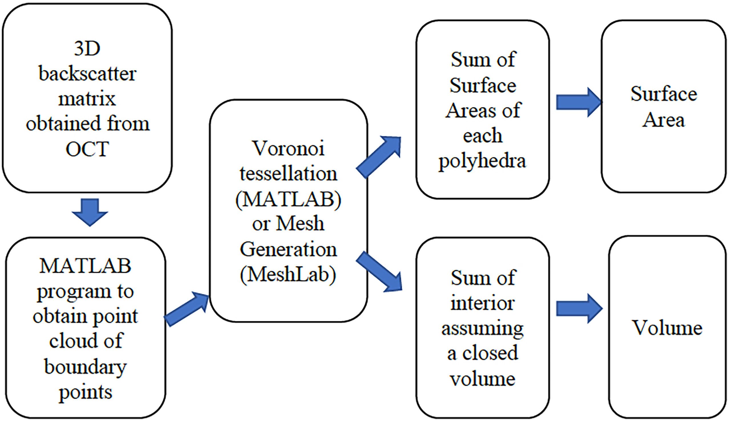
Figure 1 An overview of the processing algorithms indicating the input of OCT data, the computation of boundary points, the mesh generation or Voronoi tessellation, and the surface area and volume computations.

The SA of the exterior surface (including the bottom plane) and the volume of the polyp are then computed in MeshLab. The SA of only the upper polyp including tentacles and the polyp mouth is then used to compute the SA that is in contact with the aqueous media.

2.4 The algorithm

2.4.1 Computation of point clouds of exterior surfaces and an enclosed bottom for the polyps in MATLAB

Considering first, the “raw” data produced by the system, the field of view of the OCT system in this experiment is 7.7 mm x 3.4 mm with the depth of the scan being 2.8 mm. Given this volume, a data set of pixel dimensions (601,306,1023) was input with 3-D voxels of resolution of (12.8, 11.0, 2.7) µm. The first two dimensions here are width and length with the third dimension being depth. As a first task, to afford a simpler computation of SA and volume, the data was filtered with a 5-cubed matched filter and then resampled via cubic interpolation so that a new 3D matrix of dimension (622,1423,511) was created with a uniform spacing in 3D of 5.4 µm. Denoting the interpolated 3D volumetric data as I_p(x,y,z) , a projected view, integrated along the z axis can be computed as $I\_2d(x,y)={\displaystyle {\sum }_{z=20}^{511}{I}_p(x,y,z)}$ Note that integration was started at z = 20, as the closest values were negative due to a lack of backscatter from the air between the lens and the water. Figure 2 shows an image of I_2d(x,y) The color bar indicates that, in units of the interpolated OCT data, the integrated data values I range from 6035 to 7537. Several factors are evident that complicate the treatment of isolating the individual polyps such as overlap, tilt, and reduced values for polyps that are at a farther range from the OCT system on the tilted surface. To enable further processing, the locations, and approximate projected radii of the 17 polyps were manually identified and used to extract a set of (17) 3-D submatrices for further processing. Polyp centers were manually estimated and iteratively inspected to provide a center location as evidenced by a symmetric appearance.

FIGURE 2

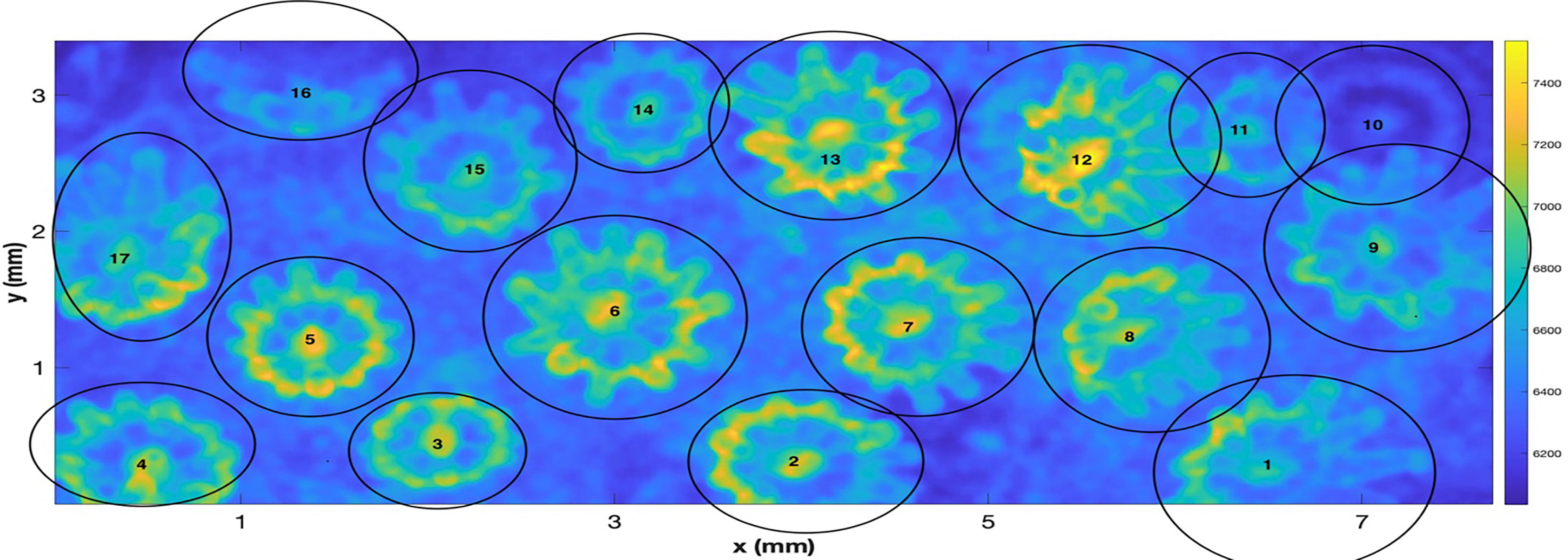
Figure 2 A “z” projected image of the “resampled data” from the 3-D OCT scan of a fragment of the coral Pocillopora damicornis. The figure shows the hand labeled centers and approximate radii of individual polyps. The scan represents an area of 3.4 mm x 7.7 mm.

Consider now the MATLAB programs that extracted the point cloud boundaries of the exterior polyp surfaces for the polyps shown in Figure 2. A detailed flow chart of the MATLAB programs is shown in Figure 3. In the next step, to increase the contrast between the coral and the surrounding water, the depth dependent backscatter of the water was estimated from a specimen free region of the coral sample. As observed, this value decreased with range, indicating that the incident beam strength decreased, given the uniform nature of the water that the corals are immersed in. This laterally unchanged, depth dependent value, was then subtracted from the data at each depth plane for the entire specimen. As a result of this step, a new 3-D data set of identical size to the entire specimen as produced. The result was to essentially zero out the backscatter from the engulfing water, thereby increasing the contrast between the coral tissue and its environment.

FIGURE 3

Figure 3 A summary of the custom MATLAB code that was used to create point clouds from the input OCT 3D matrices.

The next processing step was aimed at increasing the depth-dependent values of the backscatter from the entire corals, however, especially from parts of the substructure that are shaded by the tentacles. Hence, a column dependent normalization coefficient was computed for each (x,y) column and z dependent location. First, a range dependent function, I_T (z) is computed depth as

$\begin{array}{ll}{I}_T(z:x,y)={\displaystyle {\sum }_o^z(z:x,y)}& (1)\end{array}$

Next, a 3D normalization matrix, frac(x,y,z) was compute as

$\begin{array}{ll}frac(x,y,z)=\frac{I_T(z:x,y)}{I_{Max}}& (2)\end{array}$

where I_Max is computed as a global maximum value of the recorded data in the 3D matrix from the individual polyp after the above water removal step. We note that the values of this matrix are between 0 and 1 and it is a monotonically increasing function of depth. The frac 3D matrix was then used to multiply the data from the previous median filtering and resampling to create a new 3D data matrix as

$\begin{array}{ll}{I}_{renorm}(x,y,z)=frac(x,y,x)*I_p(x,y,z)& (3)\end{array}$

Here, the “*” operator signifies that the multiplication is carried out on an element-by-element basis. This resulted in decreasing the values of the shallower structures relative to the deeper values without increasing the noise.

The motivation for this comes from noting that if little light that is penetrating to the depths of the tissue, the value of I_ρ(x,y,z) will be very small from that depth, and the integral, I_T (z:x y) will not increase very much as a function of z. Our data analysis therefore regards the saturation of I_T (z:x y) as an indication of shading that is due to both the attenuation, likely minor at this IR wavelength, and reflection from the structures above. In the next step, the resultant 3D matrix was median filtered with a (5)³ neighborhood and the entire 3D matrix was globally binarized using the well-known Otsu algorithm.

To illustrate the results of the matrix processing, up to this point, we refer to Figure 4. The figure displays a single vertical plane, close to the polyp center, for Poly 5. Figure 4A illustrates the vertical plane after performing the initial step to subtract the depth dependent value for the water backscatter. Note that the areas not inside the polyp, and above its surface, are relatively uniformly colored, indicating that this step removed that depth dependency. Figure 4B is a slice through the 3-D frac(x,y,z). frac(x,y,z) function, computed using formula (2). Figure 4C shows the result of multiplying 4(a) by 4(b). Here, we note that the bright tips of the polyps are reduced and the shaded portions, under those tips, are of higher contrast with their surroundings. Figure 4D displays the result of using Otsu’s algorithm to create a 3-D binary matrix from the volumetric data of 4 (c). The 3-D binary matrix displays a parsimonious segmentation of the underlying structure into 2 values that is used to define the surface between the polyp and the surrounding water.

FIGURE 4

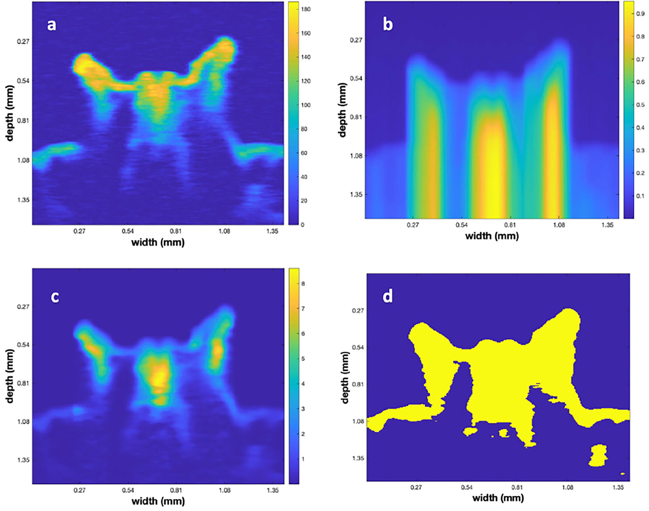
Figure 4 (A) A vertical slice through the center of polyp 5 after subtraction of the depth dependent value for water backscatter. (B) The frac matrix for the same vertical slice. (C) The results of multiplying (B) times (A). (D) Result of converting (C) to a binary image using Otsu’s method.

Given the 3-D binary matrix from Otsu’s algorithm, it is obvious that there are several rough edges in the low contrast areas. This is a natural result of the speckle noise that is a feature of all coherent imaging systems (Szkulmowski et al., 2012). To decrease their roughness, we employed a traditional algorithm, mathematical morphology (Dougherty, 2018), after filtering the data with another 3-D (5)³ median filter. We employed a set of heuristic values to accomplish the opening (with a disk or radius 3) and closing (with a disk of radius 8; Figure 5A). Next, a Canny edge detector was applied using a heuristically determined value of.45 to produce the edges that are labeled in yellow in Figure 5B. To define the top surface, a point above the polyp was used to perform a volume filling operation that filled the volume as shown in Figure 5C. In region filling, a seed value is inserted at a given (x,y,z) location, which then creates a region that grows in 3D until it is limited by defined boundaries. By planting the seed almost anywhere in the region above the polyp, assumed to be the water, the blue region above the polyp was determined as depicted in Figure 5C. However, since the MATLAB region filling (“imfill”) was only implemented in 2-dimensions, a sequence of filling was implemented on sequential planes that were chosen in the two lateral directions. The 3-D binary set of images were then logically “and-ed” to produce a new 3-D volume that was regrown in both the lateral and depth direction on plane-by-plane operation.

FIGURE 5

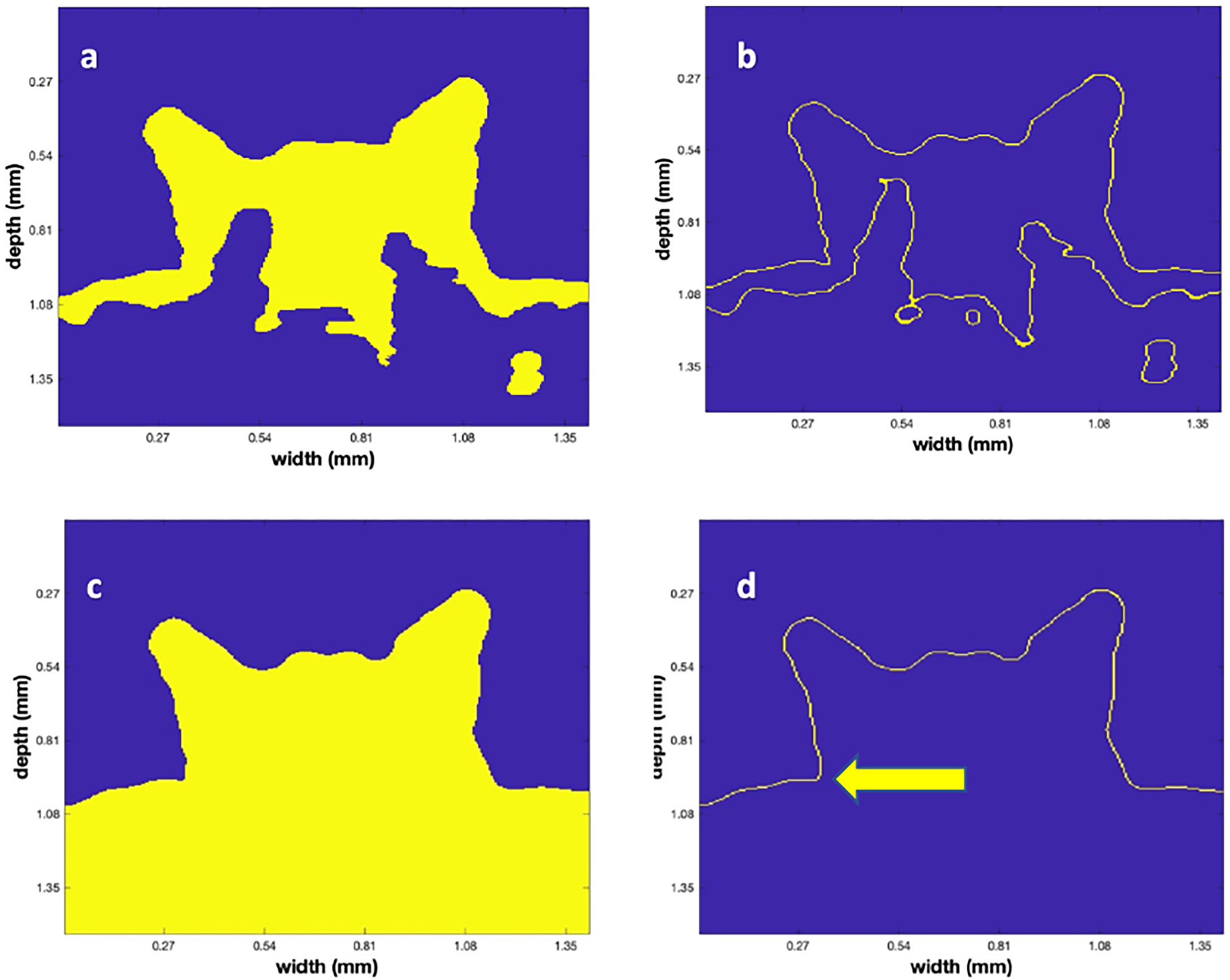
Figure 5 The successive steps in the surface identification algorithm. (A) The vertical plane, as in Figure 4D, after the mathematical morphological operations. (B) The result of applying the Canny edge detector to (A). (C) The result of the region fill operation after choosing a seed above the polyp. Note that the blue values are the filled region. (D) The final surface determined from the Canny edge detector applied to (C). The arrow indicates a vertical location that was manually chosen to be the bottom of the polyp to permit the volume calculation.

As a last step in determining the 3-D locations of the point cloud, a Canny edge detector was applied to the data shown in Figure 5C in 3D with a heuristically determined value of 0.45. The results of this operation are shown in Figure 5D. Since point clouds have both location and color value, the amplitude of the backscatter after application of the “frac” function for each of the points (that ranged from 0 – 255) in the point cloud was used and colored according to the MATLAB color map “jet” to convert from 8-bit integer values to (RGB) values in the image. Figure 6 displays a rendered 3-D picture of the point cloud that can be interactively rotated using standard MATLAB interactive functions. An animation of this rotation is provided as supplemental material (Movie 1). Note that the data was rescaled linearly so that the red values indicate a backscatter of 1 and the dark blue values are close to 0.

FIGURE 6

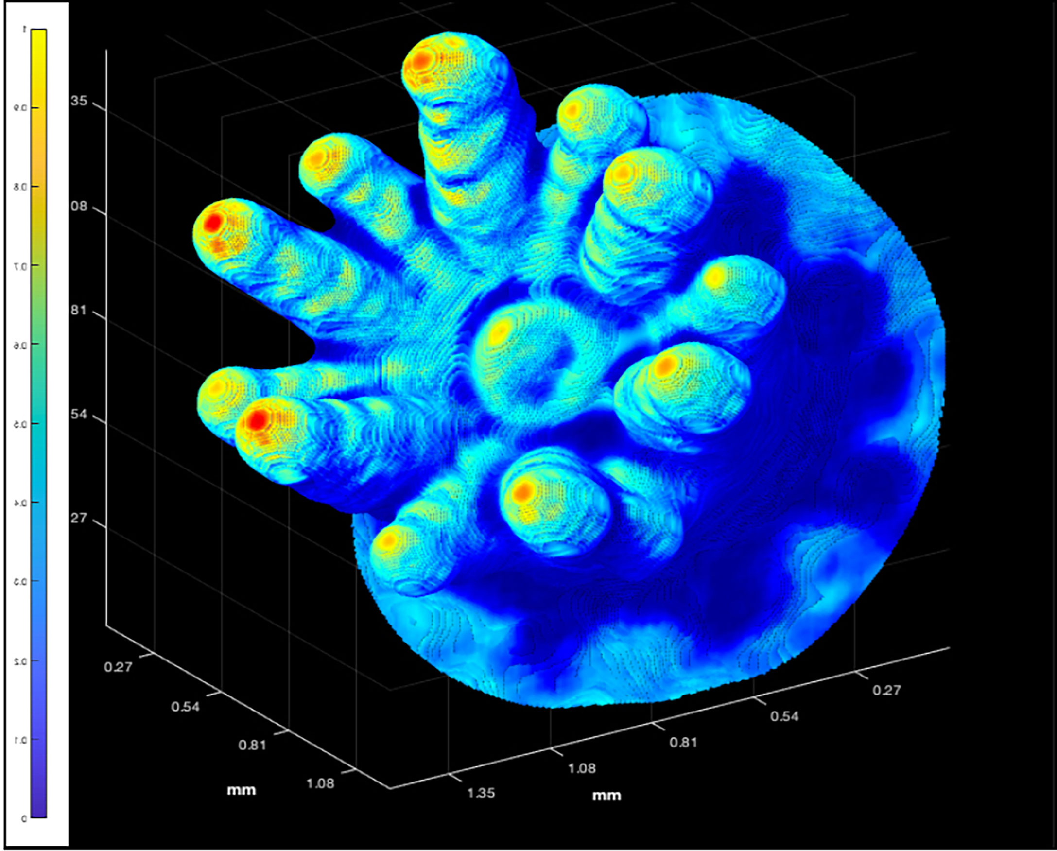
Figure 6 The 3D point cloud for an individual polyp of P. damicornis (Polyp 6 in Figure 2). The color bar highlights that the backscatter range was rescaled linearly from 1 = highest value, to 0 = lowest value, using the original backscatter values from the interpolated, unprocessed, OCT data as shading.

To calculate polyp volume an enclosed body is needed, and we thus added a horizontal plane, for each polyp, to create a bottom. The arrow in Figure 5D shows the vertical location used to construct the horizontal plane that filled the nearly circular region that was the “base” of the polyp. A region filling operation was then used to create a bottom area. This area was typically close to being circular, however, in some of the titled polyps it was more elliptical.

2.4.2 Using MeshLab to compute the volume and surface area of coral polyps

To calculate the surface area and volume of the coral polyps, the point cloud was exported in “.ply” format and input to MeshLab. The MeshLab command, “compute surface normals’ was then followed by the construction of a mesh using the “Surface Reconstruction: Screened Poisson” command. The Poisson reconstruction creates a triangular mesh from a set of 3D oriented points by solving a Poisson system that is a 3D Laplacian with positional value constraints (Kazhdan and Hoppe, 2013). After accomplishing this, a smooth mesh of the surface is then available to “compute geometrical measures” yielding both the SA and volume of the input polyp data. Since an artificial bottom was created to yield an enclosed volume, the computed volume was retained. However, the SA of the created bottom, interior to the stalk of the polyp was subtracted, so that only the external SA of stalk and the tentacles was computed. SA estimates are shown in Table 1 for polyps 5-8. The choice of these polyps was motivated since they are relatively untilted, and they are far enough away from other polyps so that we didn’t need to employ more elaborate 3D methods for extraction.

TABLE 1

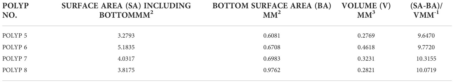
Table 1 A summary of the SA, Bottom Area, Volume as well as a ratio for the (4) polyps of the Pocillopora damicornis.

2.4.3 Computation of point clouds of exterior surfaces and an enclosed bottom for the calibration targets in MATLAB

Here, we used similar, but not identical MATLAB programs (see below), as used on the coral data to compute the SA and volume of both the borate spheres and fish eggs. In addition, the SA was analytically approximated from knowledge of observed radii to a resolution of 5.4 µm using formulas for hemi-ellipses that approximated the shapes of the spheres and eggs. Results were used to estimate the comparative accuracy of our technique.

To extract the point clouds of the calibration targets, a set of similar algorithms to those of the corals were used. One difference was that the input scan spacing was smaller (~ 1.0, 1.0, 2.74) µm. Similarly, after applying a median filter with a 5³ neighborhood, the 3D interpolation was resampled to the 5.4 µm cell resolution, identical to that of the polyps. In contrast to the above polyp processing, there was no need for subtracting a range dependent minimum value in conjunction with the range normalization matrix. The resampled data was rescaled on a depth plane by depth plane basis to yield a new 3D renormalized matrix. This was then followed by an operator, which used a circular disk that convolved with the points that were binary 0, to yield an output that closed the small discontinuities at the boundaries. Performing a gradient operator in (x, y) on each plane yielded a set of scalars that were then low pass filtered to remove noise. This replaced the Canny edge detector that was implemented in the analysis of the coral OCT data. These new matrices were used to obtain a set of binary matrices by manually choosing a thresholding value. This value was chosen via a “trial and error” procedure to get the best results for a smooth and unbiased surface, free from small particles that were attached. A region filling method was then used to fill in the “inside” of the sphere vs the “outside”, where the seed location for filling was chosen to be the apex of the sphere. A 3D edge detector and filling operations was then used to define the inside.

An additional complication was the need to estimate a maximal depth to which the data could be regarded as permitting a stable estimate of SA and Volume. We conjectured that as we regarded deeper depths, the angle between the beam and the surface became more grazing, resulting in less backscattered photons. The surface, as a function of depth, was therefore less populated with points. To solve this estimation problem, a cumulative distribution function for the number of points in the point cloud as a function of depth was computed. Inspection of this function to a cut off at which 95% of the points occurred led to an estimate of the maximal depth. We note that in almost all cases, this depth was shallower than the maximal radius or equator of the ellipsoid. However, it provided a quantitative method for determining the lowest depth plane that yielded a numerically stable surface estimate. At the end of these steps, a 3D point cloud that approximated the surface was in hand.

We then used two methods to compute the SA. In one approach, a Delaunay triangulation was used to polyhedrally approximate the surface and hence, by simple integration, the SA. This was computed in MATLAB. For comparison, a.stl file of the triangulated data was also exported to MeshLab and obtained identical results for the SA. Volume estimates were not computed, as the SA calculations indicated good agreement between the analytic SA and those computed from the Delaunay triangulation.

An additional estimate of SA was also obtained using the equation for the volume of a hemi-ellipsoid.

$\begin{array}{ll}SA\left(hemi-ellipse\right)=2*\pi *(H^{1.6075 }+{\left(SMA\right)}^{1.6075} {\left(SMI\right)}^{1.6075}){(H^{1.6075 }+{\left(SMA\right)}^{1.6075} {\left(SMI\right)}^{1.6075})}^{1/1.6075}& (4)\end{array}$

A manual estimate of height. (SMI) semi-major. (SMI) and semi-minor. (SMI) radii of the 3D ellipsoid were input to obtain the SA. The two estimates for each calibration target, analytic and Delaunay are enumerated in the results section. We also note that the solution in which the fish eggs were immersed contained many small particle fragments, which complicated the process of computing the exterior point clouds for the 3D ellipsoids. However, the use of several edge estimate techniques followed by region filling resulted in a smooth outer surface.

3 Results and discussion

3.1 Application of the method to the OCT scans of corals

To estimate both SA and volume of live coral polyps, OCT scans of four P. damicornis polyps (polyps 5, 6, 7 and 8 in Figure 2) exhibiting 3D point clouds with adequate backscatter over their entire surface area and without excessive tilting of the polyps relative to the vertically incident scan direction were analyzed. A set of 3-D renderings of the point clouds is shown in Figure 7.

FIGURE 7

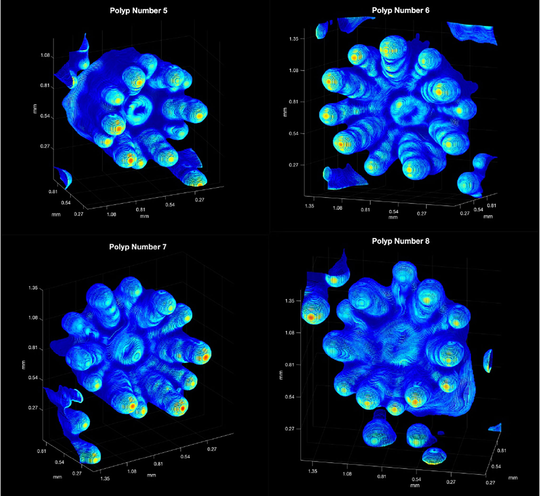
Figure 7 The computed 3D colored point clouds for the square matrices surrounding Polyps 5,6,7 and 8 (see Figure 2). The backscatter range was rescaled linearly from 1 = red (highest value), to 0 = dark blue (lowest value), using the original backscatter values from the interpolated, unprocessed, OCT data. Red implies strong backscatter and dark blue weaker backscatter. Note that point clouds from adjoining polyp are show in the periphery of the figures.

As noted above, a closed volume was needed for the volume estimation and a suitable bottom was estimated as described in Section 2.4.2. After MeshLab estimation of the SA of the entire polyp, the bottom area was subtracted to yield an estimate of polyp area. Table 1 displays the SA and volume for each of the polyps. Note that the bottom area was subtracted from the computed SA of the polyp as that was not exposed to the aqueous media. The ratio of surface area to volume for each of the polys is also shown and as evidenced, is quite close for the four polyps considered here, being close to 10 mm-1 for the four specimens considered.

3.2 Application of the method for surface definition and surface area quantification of calibration targets

Figure 8 shows the surface point clouds for 3 borate spheres (a,b,c) as well as 3 fish eggs (d,e,f). The point clouds were then tiled in MATLAB using the Delaunay triangulation, and the SA was computed via summing the created polyhedral as described above. In the case of the borate spheres, the strong surface scatter allowed easier computation of these surfaces, even in the presence of small particulates. However, the weaker scatter of the fish eggs relative to the suspended particulate matter rendered some of the fish egg data unsuitable for SA calculation.

FIGURE 8

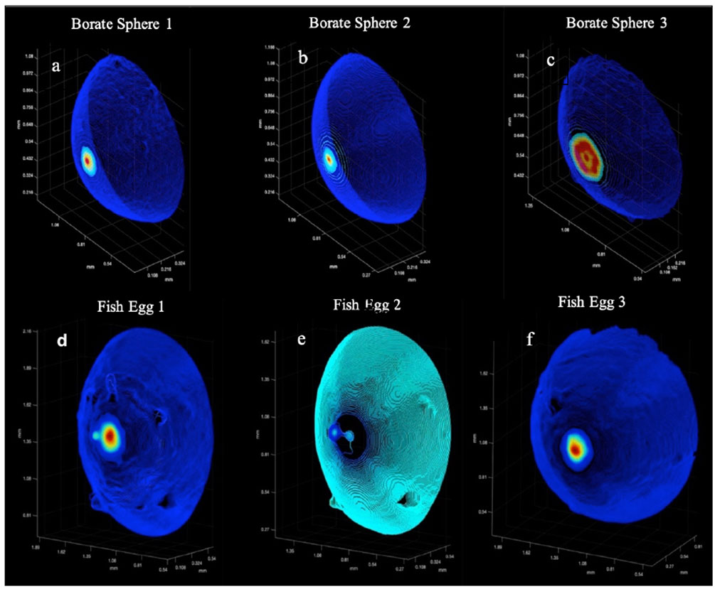
Figure 8 The calibration targets: A montage of the 3D point clouds. (A–C) are the Borate spheres. (D–F) are the Flying Fish Eggs. Color denotes backscatter strength with red as high and dark purple as low.

Table 2 contains a summary of the results of the SA calculations showing good agreement between the Delaunay and hemi-ellipsoidal results for both calibration targets. We found a linear correlation (R^{2 =} 0.93 and an intercept of 0.2) between the SA calculated from the Delaunay triangulation and the independent size measurements (Figure 9) verifying the use of these algorithms for SA determination.

TABLE 2

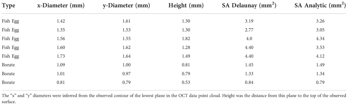
Table 2 Surface areas of borate spheres and fish eggs as determined from OCT scans and from independent size measurements.

FIGURE 9

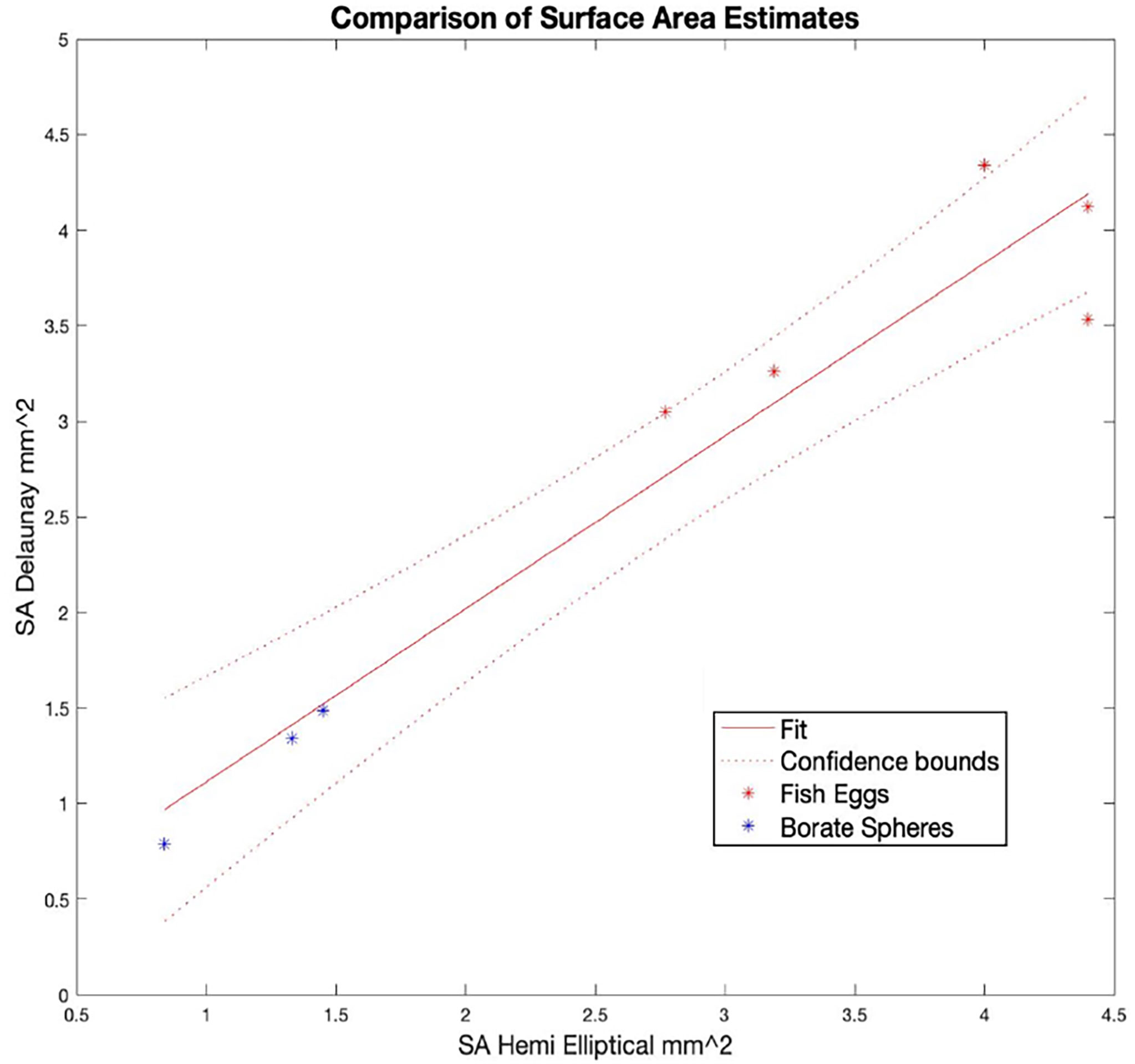
Figure 9 Comparison of surface area (SA) estimates for the calibration targets as calculated with two techniques: Delaunay triangulation of the point clouds from OCT scans that approximated the surface and the use of a formula to calculate the surface area of a 3D half ellipsoid given the lengths of the (3) semi-axes in X, Y, and Z. All data are listed in Table 1.

4 Conclusions

In conclusion, our algorithm provides a MATLAB-based pipeline for the rapid evaluation of coral tissue surface area and volume based on 3D OCT scans. Using a MacBook Pro Computer (2018, 2.7 GHz Quad-Core Intel Core i7 with 16 Gb of disk memory) the complete calculations took less than 10 minutes. The primary advantage of this approach is the high spatial resolution and non-invasive estimation of single coral polyp volume and SA. Comparable estimates at such spatial resolution cannot currently be retrieved using e.g., photogrammetry from underwater footage. However, as OCT imaging is usually based on small areas (mm to cm scale), this approach is most suitable for coral ecophysiological studies at high spatial resolution.

We also note that the maximal penetration depth is limited by the imaging system and is up to 3 mm with our commercial OCT system (Ganymede II, Thorlabs). Thus, polyp volume estimation is more suitable for thin-tissue corals such as of the family Pocilloporidae or Acroproidae. Application of our algorithm for thick-tissue corals would require the use of OCT imaging systems with enhanced penetration depth and operating at longer NIR wavelengths that await further studies.

As a further note it is interesting to speculate about what other applications there might be for the general method of using OCT to characterize the microstructure of aquatic biological organisms. In principle, any aquatic organism that has a semi-translucent (IR) surface would be a good candidate. Naturally, the relatively high resolution of ~ 5 µm will allow many of the small and important structures of a variety of organisms to be rendered with adequate detail.

Data availability statement

The raw data supporting the conclusions of this article will be made available by the authors, without undue reservation.

Author contributions

JJ, MK, and DW conceived the ideas and designed methodology; SS, DW, and JJ collected the data; JJ designed the algorithms and implemented them; JJ, MK, and DW wrote the manuscript. All authors contributed to the article and approved the submitted version.

Funding

This study was supported by grants from the National Science Foundation (17-36799, JJ), the European Union’s Horizon 2020 research and innovation program (702911-BioMIC-FUEL, DW), the Gordon and Betty Moore Foundation through grant #93225 (DW) and #GBMF9206 (MK) (https://doi.org/10.37807/GBMF9206), and the Carlsberg Foundation (MK, CF14-0573 grant).

Conflict of interest

The authors declare that the research was conducted in the absence of any commercial or financial relationships that could be construed as a potential conflict of interest.

Publisher’s note

All claims expressed in this article are solely those of the authors and do not necessarily represent those of their affiliated organizations, or those of the publisher, the editors and the reviewers. Any product that may be evaluated in this article, or claim that may be made by its manufacturer, is not guaranteed or endorsed by the publisher.

Supplementary material

The Supplementary Material for this article can be found online at: https://www.frontiersin.org/articles/10.3389/fmars.2022.1049440/full#supplementary-material

References

Bythell J., Pan P., Lee J. (2001). Three-dimensional morphometric measurements of reef corals using underwater photogrammetry techniques. Coral reefs 20 (3), 193–199. doi: 10.1007/s003380100157

CrossRef Full Text | Google Scholar

Dougherty E. (2018). Mathematical morphology in image processing. vol. 1.

Google Scholar

Drexler W., Fujimoto J. G. (2015). Optical coherence tomography: technology and applications (Vol. 2) (Berlin: Springer). doi: 10.1007/978-3-540-77550-8

CrossRef Full Text | Google Scholar

Fercher A. F., Drexler W., Hitzenberger C. K., Lasser T. (2003). Optical coherence tomography-principles and applications. Rep. Prog. Physics. 66 (2), 239. doi: 10.1088/0034-4885/66/2/204

CrossRef Full Text | Google Scholar

Fiske L. D., Aalders M. C., Almasian M., van Leeuwen T. G., Katsaggelos A. K., Cossairt O., et al. (2021). Bayesian Analysis of depth resolved OCT attenuation coefficients. Sci. Rep. 11 (1), 1–11. doi: 10.1038/s41598-021-81713-7

PubMed Abstract | CrossRef Full Text | Google Scholar

Hoegh-Guldberg O. (1988). A method for determining the surface area of corals. Coral Reefs. 7 (3), 113–116. doi: 10.1007/BF00300970

CrossRef Full Text | Google Scholar

Huang D., Swanson E. A., Lin C. P., Schuman J. S., Stinson W. G., Chang W., et al. (1991). Optical coherence tomography. Science 254 (5035), 1178–1181. doi: 10.1016/B978-0-323-02346-7.50008-9

PubMed Abstract | CrossRef Full Text | Google Scholar

Hughes J. F., Van Dam A., McGuire M., Foley J. D., Sklar D., Feiner S. K., et al. (2014). Computer graphics: principles and practice (Pearson Education).

Google Scholar

Kaandorp J. A., Kübler J. E. (2001). The algorithmic beauty of seaweeds, sponges and corals (Springer Science & Business Media). doi: 10.1007/978-3-662-04339-4

CrossRef Full Text | Google Scholar

Kazhdan M., Hoppe H. (2013). Screened poisson surface reconstruction. ACM Trans. Graphics (ToG) 32 (3), 1–13. doi: 10.1145/2487228.2487237

CrossRef Full Text | Google Scholar

Khatamian A., Arabnia H. R. (2016). Survey on 3D surface reconstruction. J. Inf. Process. Syst. 12 (3), 338–357. doi: 10.3745/JIPS.01.0010

CrossRef Full Text | Google Scholar

Koch H. R., Wallace B., DeMerlis A., Clark A. S., Nowicki R. J. (2021). 3D scanning as a tool to measure growth rates of live coral microfragments used for coral reef restoration. Front. Mar. Sci 420. doi: 10.3389/fmars.2021.623645

CrossRef Full Text | Google Scholar

Laissue P. P., Roberson L., Gu Y., Qian C., Smith D. J. (2020). Long-term imaging of the photosensitive, reef-building coral acropora muricata using light-sheet illumination. Sci. Rep. 10, 10369. doi: 10.1038/s41598-020-67144-w

PubMed Abstract | CrossRef Full Text | Google Scholar

Lange I. D., Perry C. T. (2020). A quick, easy and non-invasive method to quantify coral growth rates using photogrammetry and 3D model comparisons. Methods Ecol. Evol. 11 (6), 714–726. doi: 10.1111/2041-210X.13388

CrossRef Full Text | Google Scholar

Lavy A., Eyal G., Neal B., Keren R., Loya Y., Ilan M. (2015). A quick, easy and non-intrusive method for underwater volume and surface area evaluation of benthic organisms by 3D computer modelling. Methods Ecol. Evol. 6 (5), 521–531. doi: 10.1111/2041-210X.12331

CrossRef Full Text | Google Scholar

Marsh J. A. (1970). Primary productivity of reef-building calcareous red algae. Ecology 51, 255–263. doi: 10.2307/1933661

CrossRef Full Text | Google Scholar

Meshlab (2021). Available at: https://www.meshlab.net.

Google Scholar

Naumann M. S., Niggl W., Laforsch C., Glaser C., Wild C. (2009). Coral surface area quantification–evaluation of established techniques by comparison with computer tomography. Coral reefs 28 (1), 109–117. doi: 10.1007/s00338-008-0459-3

CrossRef Full Text | Google Scholar

Odum H. T., Odum E. P. (1955). Trophic structure and productivity of a windward coral reef community on eniwetok atoll. Ecol. Monogr. 25 (3), 291–320. doi: 10.2307/1943285

CrossRef Full Text | Google Scholar

Patterson M. R. (1992). A chemical engineering view of cnidarian symbioses. Am. Zoologist. 32 (4), 566–582. doi: 10.1093/icb/32.4.566

CrossRef Full Text | Google Scholar

Pollefeys M., Van Gool L., Vergauwen M., Verbiest F., Cornelis K., Tops J., et al. (2004). Visual modeling with a hand-held camera. Int. J. Comput. Vision 59 (3), 207–232. doi: 10.1023/B:VISI.0000025798.50602.3a

CrossRef Full Text | Google Scholar

Raz-Bahat M., Faibish H., Mass T., Rinkevich B. (2009). Three-dimensional laser scanning as an efficient tool for coral surface area measurements. Limnology Oceanography: Methods 7 (9), 657–663. doi: 10.4319/lom.2009.7.657

CrossRef Full Text | Google Scholar

Spicer G. L. C., Eid A., Wangpraseurt D., Swain T. D., Winkelmann J. A., Yi J., et al. (2019). Measuring light scattering and absorption in corals with inverse spectroscopic optical coherence tomography (ISOCT): a new tool for non-invasive monitoring. Sci. Rep. 9 (1), 1–12. doi: 10.1038/s41598-019-50658-3

PubMed Abstract | CrossRef Full Text | Google Scholar

Stimson J., Kinzie R. A. III (1991). The temporal pattern and rate of release of zooxanthellae from the reef coral pocillopora damicornis (Linnaeus) under nitrogen-enrichment and control conditions. J. Exp. Mar. Biol. Ecol. 153 (1), 63–74. doi: 10.1016/S0022-0981(05)80006-1

CrossRef Full Text | Google Scholar

Szkulmowski M., Gorczynska I., Szlag D., Sylwestrzak M., Kowalczyk A., Wojtkowski M. (2012). Efficient reduction of speckle noise in optical coherence tomography. Optics express 20 (2), 1337–1359. doi: 10.1364/OE.20.001337

PubMed Abstract | CrossRef Full Text | Google Scholar

Vermeer K. A., Mo J., Weda J. J., Lemij H. G., de Boer J. F. (2014). Depth-resolved model-based reconstruction of attenuation coefficients in optical coherence tomography. Biomed. Optics Express. 5 (1), 322–337. doi: 10.1364/BOE.5.000322

CrossRef Full Text | Google Scholar

Wagner M., Horn H. (2017). Optical coherence tomography in biofilm research: A comprehensive review. Biotechnol. Bioengineering 114 (7), 1386–1402. doi: 10.1002/bit.26283

CrossRef Full Text | Google Scholar

Wangpraseurt D., Jacques S., Lyndby N., Holm J. B., Pages C. F., Kühl M. (2019). Microscale light management and inherent optical properties of intact corals studied with optical coherence tomography. J. R. Soc. Interface 16 (151), 20180567. doi: 10.1098/rsif.2018.0567

PubMed Abstract | CrossRef Full Text | Google Scholar

Wangpraseurt D., Larkum A. W., Ralph P. J., Kühl M. (2012). Light gradients and optical microniches in coral tissues. Front. Microbiol. 3. doi: 10.3389/fmicb.2012.00316

PubMed Abstract | CrossRef Full Text | Google Scholar

Wangpraseurt D., Wentzel C., Jacques S. L., Wagner M., Kühl M. (2017). In vivo imaging of coral tissue and skeleton with optical coherence tomography. J. R. Soc. Interface 14 (128), 20161003. doi: 10.1098/rsif.2016.1003

PubMed Abstract | CrossRef Full Text | Google Scholar

Yoo K. M., Tang G. C., Alfano R. R. (1990). Coherent backscattering of light from biological tissues. Appl. Optics 29 (22), 3237–3239. doi: 10.1364/AO.29.003237

CrossRef Full Text | Google Scholar

Zawada K. J., Dornelas M., Madin J. S. (2019). Quantifying coral morphology. Coral Reefs 38 (6), 1281–1292. doi: 10.1007/s00338-019-01842-4

CrossRef Full Text | Google Scholar