The generation mechanism of cold eddies and the related heat flux exchanges in the upper ocean during two sequential tropical cyclones

1. Introduction

The passage of a tropical cyclone (TC) over the warm ocean represents a typical part of air-sea interactions and has strong dynamic and thermal impacts on the upper ocean (Price et al., 1994; Cheng et al., 2015; Potter et al., 2017). And the influence of a TC on the ocean can be divided into two stages, namely forced stage and relaxation stage. During the forced stage, the “resonance effect” between TC wind stresses and ocean currents generates near-inertial oscillation. This is due to strong shear stress across the base of the mixed-layer, which will induce vertical mixing (Mayer et al., 1981). After the passage of the TC, the ocean will enter the relaxation stage. During the relaxation stage, the ocean response is mainly affected by inertial gravity oscillation excited by the TC. The mixed-layer velocity oscillates with a near-inertial period. As a result, sea surface currents diverge and produce upwelling (Tsai et al., 2008). Vertical mixing largely explains sea surface cooling and air-sea heat flux exchanges. However, TC-induced deeper and cooler upwelling also plays a role, as it partly balances the warming of subsurface water caused by vertical mixing. So a combination of vertical mixing and upwelling causes a redistribution of heat in the upper ocean (Prasad and Hogan, 2007; Jaimes and Shay, 2009). Concurrently, a decrease in the sea surface temperature (SST) and a change in upper ocean heat content also have a significant negative feedback effect on the TCs intensity, weakening or reducing the energy supplied to TCs (Park et al., 2019). Moreover, the distribution of phytoplankton biomass is influenced by TCs. TCs cause intense Ekman pumping velocity (EPV), elevating nutrient-rich or chlorophyll a (chl-a)-rich water up to the euphotic layer, thereby promoting an overall increase in the surface chl-a concentration and improving primary productivity (Babin et al., 2004).

Besides, according to previous studies, the cyclonic eddy was generated by a slow-moving and looping track typhoon, or along the tracks of binary typhoons (Hu and Kawamura, 2004; Yang et al., 2012). These studies show that the passage of certain typhoons, such as looping track typhoons or binary typhoons, may play a significant role in inducing cold eddies generation.

In addition, along with the generation of cyclonic eddies, a series of physical processes occur inside the cyclonic eddies along their vertical profile, including eddy pumping, eddy stirring, eddy trapping, etc. That makes heat flux exchanges inside the cyclonic eddies more prominent (Zhang et al., 2019). As Yang et al. (2015) found that inside a cold eddy, the maximum cooling of up to 2°C can be caused between 60 dbar and 80 dbar. What’s more, TCs usually pass through mesoscale ocean eddy fields and inject obvious disturbances during their movement (Lu et al., 2016). The intensity, size and vertical structure of a preexisting eddy can also be modified by the TC (Lu et al., 2020). Meanwhile, changes in the eddy caused by the TC can also enhance the ocean’s response to the TC. Qiu et al. (2021) analyzed TC Bailu led to SST decrease within the cold eddy and enlarge the size of the cold eddy. Then the cooled-enlarged eddy excited heat advection transport reached -0.4/day. This has a certain contribution to the extreme cooling of the sea surface when the TC Bailu passes through.

In addition, when the cold eddy moves, if the ratio of the rotational speed U of the cold eddy to its propagation speed c (i.e., U/c) is greater than 1, the cold eddy can be considered a moving water mass. It plays an essential role in modulating ocean general circulation and marine biochemical processes. And it also plays a significant role in the zonal conduction of heat and salt (Gilson and Roemmich, 2001; Qiu and Chen, 2005).

Due to the severe weather conditions during the passage of TCs, it is very difficult to monitor the complete TC transit process and to obtain real-time data. Therefore, various models have also been widely used to study TCs all over the world. For example, the WRF model is one of the most popular regional numerical weather prediction models being used by operational and research personnel. It also has the advantages of flexibility, dynamic and easy access to physical options. Recent sensitivity experiments by various researchers have also verified that the WRF model is one of the best performing mesoscale models for reproducing TC development (Cheng and Steenburgh, 2005; Davis et al., 2008).

From a climatological point of view, TCs in the Arabian Sea (AS) have distinct features and exhibit strong differences from those in other basins. The annual cycle of AS TCs is characterized by prominent double peaks occurring during the monsoon transition periods (April-May and October-November) (Mohapatra et al., 2017). Moreover, on average, there are approximately two TCs in the AS each year. Therefore, the AS region has a high frequency of TC passage (Evan and Camargo, 2011).

The aim of this study is to determine the generation mechanism of cold eddies and related heat flux exchanges in eddy fields during two sequential TCs: TC Kyarr (October 2019) and TC Maha (November 2019) over the AS. This paper is organized as follows: section 2 provides a detailed description of the WRF model simulation and the experimental design; section 3 contains a description of the data and methods; section 4 gives the results and discussion; finally, section 5 presents the conclusion.

2. WRF model experimental design

In this experiment, the WRF model is adopted for the physical parametric scheme of TC simulation, as shown in Table 1. The TCs Kyarr and Maha, which landed in the northern Indian Ocean in 2019, are selected as experimental cases, and the simulation periods are 18:00 UTC October 24 to 00:00 UTC November 01, 2019, and 06:00 UTC October 30 to 12:00 UTC November 06, 2019, respectively. The centre of the simulated region is located at (13.2°N, 78.8°E), and the Mercator projection is adopted. The dimensions of the grid in the D01 area are 196×129, and the horizontal resolution is 54 km; the dimensions of the grid in the D02 area are 328×217, and the horizontal resolution is 18 km. There are 50 vertical layers, and the vertical top height is 50 hPa. During the TC simulation, the information of TC location and fixed intensity is output every three hours as a model to simulate the location and intensity of TCs.

TABLE 1

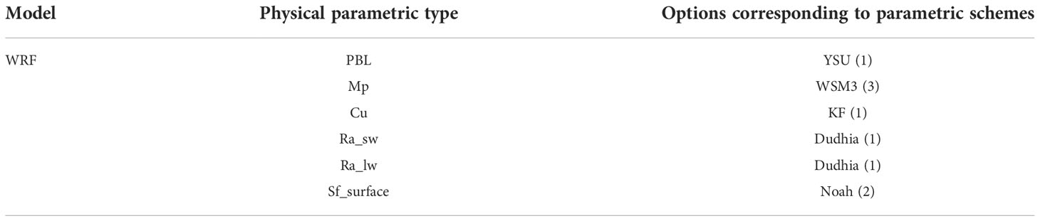
Table 1 Specific options of the default parametric scheme.

3. Data and methods

3.1. Data

3.1.1. TC track data and intensity

Information on Kyarr and Maha is obtained from the best track datasets of the Joint Typhoon Warning Center (JTWC, http://www.usno.navy.mil/NOOC/nmfc-ph/RSS/jtwc/best_tracks). This includes the centre location, the minimum sea surface pressure, the maximum sustained wind speed and the wind radius [at the radius of specified wind (17 m/s)] in every 6-hour interval.

3.1.2. Analysis and reanalysis data

The European Center for Medium-Range Weather Forecasts (ECMWF) ERA5 fifth-generation atmospheric reanalysis data of the global climate represent the detailed evolution of weather systems. ERA5 data have very high spatial and temporal resolutions. This product is widely used to analyse the evolution of TCs. In this study, the 10 m U-component of wind, 10 m V-component of wind and sea surface pressure from ERA5 data with a spatial resolution of 0.25°× 0.25° and a temporal resolution of one hour were used. The ERA5 data, which cover data from 1979 to present, are now available for public use. Detailed documentation and download information can be found at the ECMWF website (https://www.ecmwf.int/).

The daily SST product used in this study is obtained from NOAA Global Surface Temperature Data (NOAA Global Temp) with a 1/4 degree global grid. It combines global SST data with global land surface air temperature data into merged data of both the land and ocean surface temperature (available at https://psl.noaa.gov/data/gridded/data.ncep.reanalysis.derived.surface.html/).

3.1.3. Remote sensing data

The daily chl-a concentration data are merged with satellite-derived altimeter products from multiple satellite sensor observations. The daily altimeter-derived sea surface height anomaly and sea surface currents data are provided by Archiving, Validation and Interpretation of Satellite Data in Oceanography (AVISO). All of these products have a spatial resolution of 4 km and are produced and distributed by the Copernicus Marine Environmental Monitoring Center (CMEMS, http://marine.copernicus.eu/).

3.1.4. In situ observations

In this study, the upper ocean temperature and salinity measured by Argo floats are taken from the India Argo project (ftp://ftp.ifremer.fr/ifremer/argo). All these Argo floats are equipped with conductivity–temperature–depth (CTD) sensors and deployed in the AS to collect ocean data at 10-day intervals from depths of 5 m to 2000 m as a part of the Argo program.

The ocean temperature and salinity data are recorded by the Argo floats, and quality control is performed. The Argo float profiles before and after the passage of the two sequential TCs along their tracks are selected. This provides a good opportunity to study changes in the upper ocean environments induced by TCs. The locations and observation periods of the five Argo floats distributed near the TC tracks adopted in this study are shown in Figures 1B, 2F.

3.1.5. Model data

Data with a spatial resolution of 0.08°x0.08° from the global HYbrid Coordinate Ocean Model (HYCOM, https://www.hycom.org/) daily and hourly numerical model outputs are driven by the Navy Environmental Model version 1.2 (Chassignet et al., 2007). Data of three-dimensional ocean temperature and salinity are used in this study to show temperature profile changes with time during TC passage and to calculate the density of sea water, MLD, and heat flux exchanges at different layers in the upper ocean.

3.2. Methods

3.2.1. Wind stress curls

The wind stress curls play an important role in the dynamic processes of the upper ocean during the passage of TC. For example, wind stress curls cause sea water to converge and diverge, with corresponding changes in sea surface height (Chiang et al., 2011). To better understand this role, the wind stress curls are computed based on the wind stresses. The wind stresses are given by:

$\begin{array}{ll}\tau =\rho a{C}_D\left|\overrightarrow{U}\right|\overrightarrow{U}& (1)\end{array}$

ρa is the density of air, $\overrightarrow{U}$ is the wind speed 10 m over the sea surface, and CD is the drag coefficient (Powell et al., 2003). The drag coefficient is calculated as follows:

$\begin{array}{ll}{C}_D=[\begin{array}{l}1.2x{10}^{-3},0\le \overrightarrow{U}<11m/s\\ (0.49+0.065\overrightarrow{U})x{10}^{-3},11\le \overrightarrow{U}\le 25m/s\\ 2.115x{10}^{-3},\overrightarrow{U}>25m/s\end{array}& (2)\end{array}$

The wind stress curls (W) are calculated as:

$\begin{array}{ll}W=\frac{\partial \tau y}{\partial x}-\frac{\partial \tau x}{\partial y}& (3)\end{array}$

τy and τx are the meridional and zonal wind stresses, respectively, ∂x and ∂y are the distances in the west-east and south-north directions, respectively.

3.2.2. Maximum forcing time and maximum adjustment time

The method of Sun et al. (2010) is used to divide the wind field data into half-hour intervals along the TC tracks data provided by JTWC, and the forcing time of TC is calculated, which is defined as the wind speed of TC (wind speed > 17 m/s) blowing time at the sea surface.

According to Gill et al. (1974) geostrophic adjustment theory, the adjustment time is at least 1/f , in which f=2ωsinθ is the Coriolis force, where ω is the Earth’s angular velocity and = 7.292x10^-5 rad/s and θ is the local latitude. In this study, after Kyarr and Maha passed through, the maximum adjustment time of three cold eddies is calculated (November 07, 2019).

3.2.3. Eddy detection algorithms

Among the eddy detection methods based on physical parameters, the Okubo-Weiss (OW) parametric method has been widely used (Okubo, 1970), but this method also has some disadvantages. Therefore, Nencioli et al. (2010) further improved the eddy detection method based on Euler-type data and categorized it into four constraints:

1. Along an east–west (EW) section, zonal v components of currents velocity, v has to reverse in sign across the eddy centre, and its magnitude has to increase moving away from the centre;

2. Along a north–south (NS) section, meridional u components of currents velocity, u has to reverse in sign across the eddy centre, and its magnitude has to increase moving away from the centre; the sense of rotation has to be the same as that of v;

3. The velocity magnitude exhibits a local minimum at the eddy centre;

Based on the above, after the eddy centre is determined, the outermost closed line is determined to be the boundary of the eddy according to the flow function of the eddy region, and the average distance from the eddy boundary point to the eddy centre is defined as the eddy radius.

3.2.4. Sea surface relative vorticity

During the passage of the TC, the strong wind stresses of the TC can easily cause the geostrophic balance of sea surface to be lost and cause vorticity anomalies (Wang et al., 2007). Moreover, cyclonic eddy often shows positive vorticity, so calculating the change in the relative vorticity of sea surface helps reveal the generation mechanism of the cyclonic eddy.

$\begin{array}{ll}\zeta =\frac{\partial v}{\partial x}-\frac{\partial u}{\partial y}& (4)\end{array}$

where v and u are two components of the sea surface currents along the west–east and south–north directions, respectively, ∂x and ∂y are the distances in the west–east and south–north directions, respectively.

3.2.5. Nondimensional numbers

Some nondimensional numbers, such as the nondimensional storm speed, S, are calculated to aid understanding of the general characteristics of each TC. S, which is the ratio of the local inertial period to the residence time of a TC. The value of S is considered an indication of the timescale at which the ocean is subjected to the TC strong wind stresses compared to the local inertial period. Thus, this is an indication of the near-inertial ocean response generated by a TC. Following Price et al. (1994), S is defined as:

$\begin{array}{ll}S=\frac{\pi Uh}{4fR\max }& (5)\end{array}$

R_max is the radius to maximum wind stress. U_h is the TC’s translation speed.

The Burger number, B. B, is a direct measure of the degree of pressure coupling between mixed-layer currents and thermocline currents. As shown in the following formula, the decay and e-folding time for mixed-layer currents (through energy dispersion) are directly dependent on the Burger number (Price et al., 1994).

$\begin{array}{ll}B=\frac{g\text{'}h\max }{4f{R}^2\max }& (6)\end{array}$

$\begin{array}{ll}g\text{'}=\frac{g\Delta \rho }{\rho 0}& (7)\end{array}$

g' is the reduced gravity. Δρ is the density difference across the seasonal thermocline. ρ0 is the density of mixed-layer, and the MLD is defined here as the depth where the temperature is 0.5°C less than the SST (Kara et al., 2000). g = 9.8 m/s² is the acceleration due to gravity, hmax is the maximum MLD.

C, is the ratio of the translation speed of the TC to the gravest mode internal wave phase speed. And the Mach number indicates significant upwelling directly beneath the TC and includes a substantial geostrophic component. The upwelling driven by wind stress curls is the most important process. It causes the variation of thermocline density through the divergence of upper layer transport. The Mach number C, as given by Price et al. (1994):

$\begin{array}{ll}C=\frac{Uh}{c}& (8)\end{array}$

C is the gravest mode internal wave phase speed, with a nominal value of c=2m/s

4. Results and discussion

4.1. Comparison of TC tracks evolution

The results from the WRF model simulation of two sequential TCs Kyarr and Maha are presented in this section. The JTWC and ERA5 estimate basic tropical cyclone data at every 6h can be observed, though in situ observations during tropical cyclone events in the Arabian Sea region are lacking. The tracks which TCs Kyarr and Maha were observed and simulated are presented in Figures 1A, B. In ERA5, WRF model simulation, the centers of Kyarr and Maha are located at the minimum point of sea level pressure. In Figures 4A, B, the tracks of Kyarr, Maha provided by JTWC, ERA5, WRF model simulation all show that TCs first moved to the northwest and then changed abruptly. In general, the TC tracks provided by ERA5 are basically consistent with those provided by JTWC. As would be observed, there is a significant difference between the WRF model simulation and ERA5, JTWC. For example, the WRF model simulation track of TC Kyarr biased to the west side of the observed track at first. Then the track was greatly biased to the east side of the observed track after it’s sudden change. Though deviating from the Maha’s observed track at the beginning, it’s track changes were basically consistent with those provided by ERA5 and JTWC afterwards. In another study, it was found a higher track deviation might be attributed to the initial positioning error (Osuri et al., 2012). In general, the WRF model simulation exhibits relatively large errors in the track of TC Kyarr. Unlike TC Maha, the WRF model simulation has a relatively high consistency with the track provided by JWTC and ERA5. From the above, in this paper, we will use the tracks provided by JTWC as the tracks of TCs Kyarr and Maha.

FIGURE 1

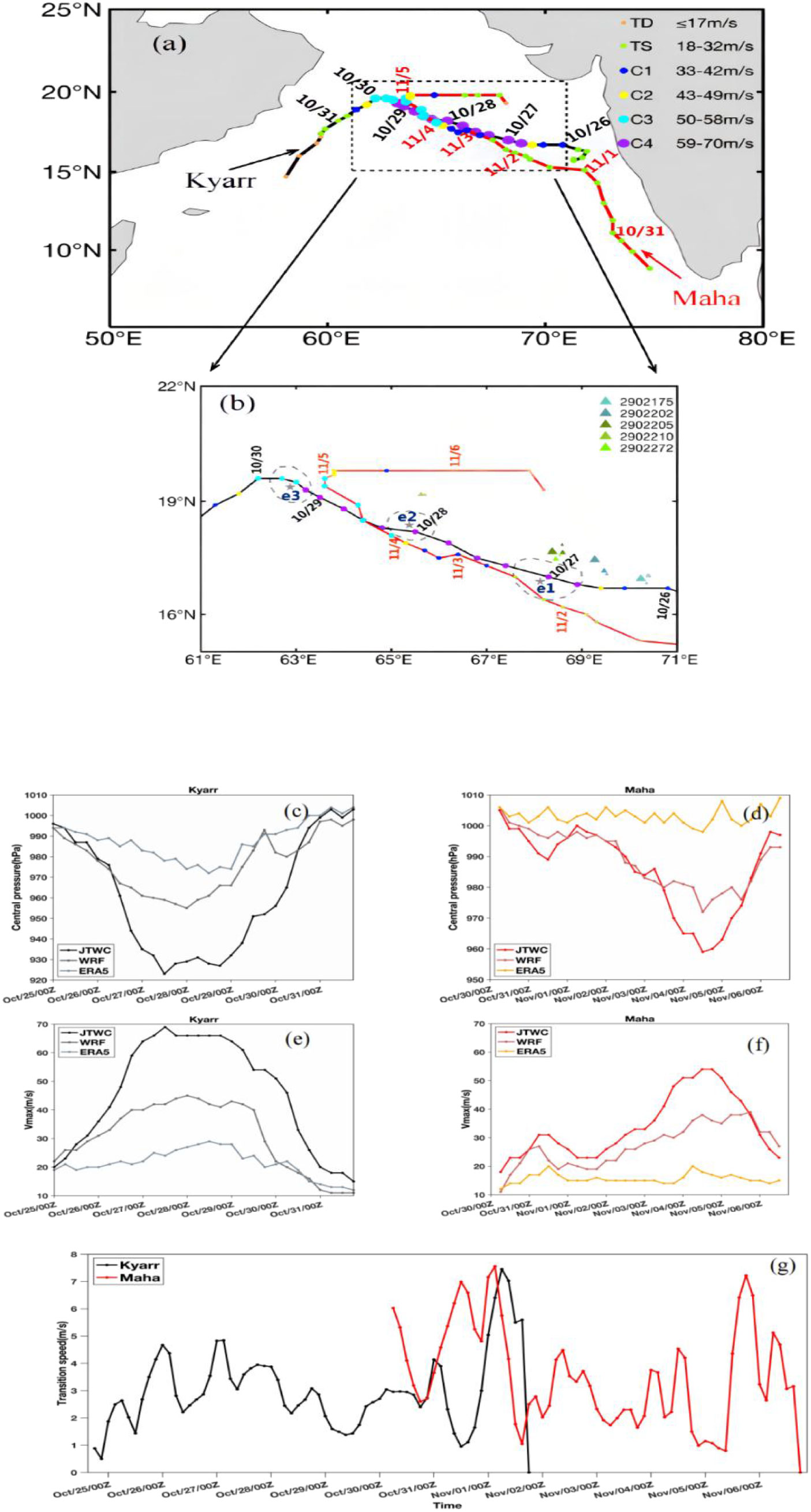
Figure 1 Tracks (A, B), intensities according to JTWC, WRF model simulation, and ERA5 (C–F) and translation speeds (G). In (A, B), the black and red lines represent the tracks of TCs Kyarr and Maha, respectively. The colours of circles indicate the intensity of TCs (according to the Saffir-Simpson hurricane scale), and the interval of each circle is 6 hours. The grey dotted lines represent the eddy shapes, the grey five-pointed stars represent the eddy centres of cyclonic eddies e1, e2, and e3 (November 07, 2019, by eddy detection algorithms). The temporal and spatial variations in the Argo floats are represented by various coloured triangle symbols. The small (large) symbols represent the location of Argo floats pre (post)-TC Kyarr.

4.2. Two sequential tropical cyclones in October 2019

The tracks, intensities and translation speeds of Kyarr and Maha in October 2019 are shown in Figures 1A–G. TCs Kyarr and Maha followed a similar path across the AS from October 24 to November 06, 2019. First, Kyarr originated and reached tropical storm status on the night of 25 October 2019 near India (Figure 1A). Then Kyarr moved north-westwards continuously developed from 00:00 UTC to 18:00 UTC on October 26, and it quickly strengthened from Category 1 to Category 4. The Category 4 stage persisted for approximately 54 hours according to the Saffir-Simpson scale.

FIGURE 2

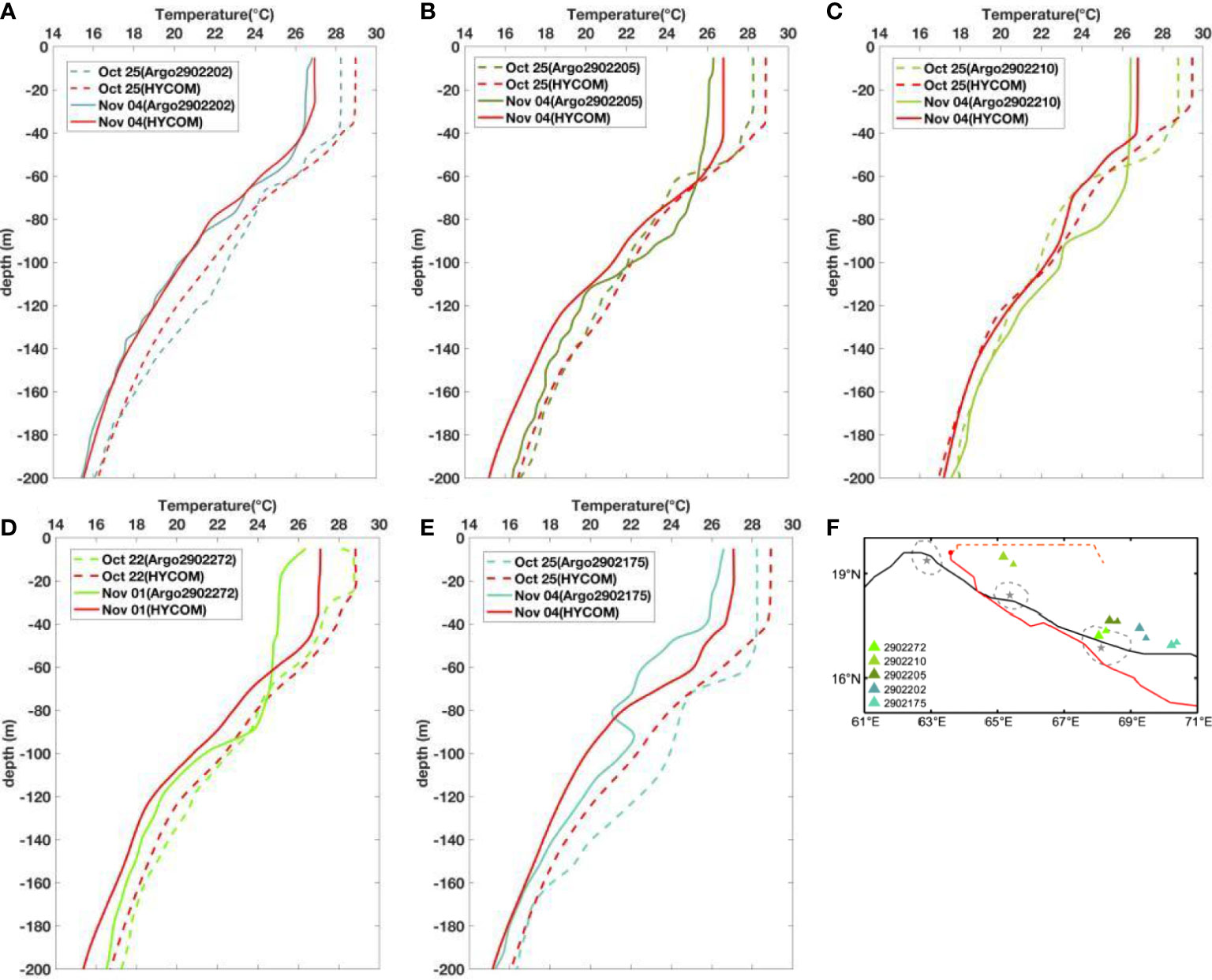
Figure 2 (A–E) show a comparison of temperature profiles obtained from Argo observations (different colours represent different Argo floats) and HYCOM model output results at different times. In (F) The Argo floats are represented by various coloured symbols. The small(large) symbols represent the location of Argo floats pre (post)-TC Kyarr/Maha. The grey dotted lines represent the shape and eddy centre of cyclonic eddies e1, e2, and e3 (November 07, 2019, eddy detection algorithms detected). The Argo floats are represented by various coloured symbols. The expression of TC tracks is the same as that in Figure 3. The red solid point represents the location of TC Maha on November 04.

At noon on October 29, Kyarr made a sudden south-westerly turn and gradually weakened before dissipating into a tropical storm and finally disappearing over the western AS. Afterwards, a week after Kyarr originated, Maha originated in the sea near southern India and moved north-westwards. Later, Maha was upgraded to Category 1 on the evening of November 02 and gradually strengthened to reach its maximum intensity of Category 3 in the early morning of November 04. Approximately a day after Maha continued moving northwest as a Category 3 TC, the track of Maha changed to the east near the area where Kyarr suddenly turned. Finally, Maha gradually weakened and disappeared over the northern AS.

For the purpose of comparing the WRF model simulation results, the minimum central pressure and maximum sustained wind speed from JTWC and ERA5 were used (Figures 1C–F). The maximum 10 m wind speed from the WRF model simulation and ERA5 were used as the maximum sustained wind speed.

Notably, the TCs intensity indicated by ERA5 appears to be particularly weak compared to the intensity indicated by JTWC and WRF model simulation. Moreover, the WRF model simulation and ERA5 peaks (maximum sustained wind speed and minimum central pressure) were delayed relative to those of JTWC. However, according to the evolution of minimum central pressure recorded by JTWC, WRF model simulation and ERA5 for Kyarr and Maha, the minimum central pressure values of TC Kyarr were 923 hPa, 955, and 974 hPa, respectively (Figure 1C). The JTWC-recorded minimum central pressure for TC Maha was 959 hPa, that recorded by WRF model simulation and ERA5 were 972 and 998 hPa, respectively (Figure 1D). For the maximum sustained wind speed of Kyarr and Maha, JTWC maximum sustained wind speed were faster than WRF model simulation and ERA5. And the JTWC-recorded maximum sustained wind speed for TC Kyarr was 69 m/s, while that of WRF model simulation and ERA5 were 45 and 29 m/s, respectively (Figure 1E). Moreover, the maximum sustained wind speed of TC Maha recorded by JTWC was 54 m/s, while that recorded by WRF model simulation and ERA5 were 39 and 20 m/s, respectively (Figure 1F). The WRF model simulation underestimated the minimum central pressure and maximum sustained wind speed during the development stage compared to that of JTWC but was closer to ERA5.

The translation speeds of Kyarr and Maha were calculated according to the locations of the TCs centres in the time series (Figure 1G). Kyarr moved relatively slowly (1–4 m/s) during most stages over the AS. Maha moved relatively fast during the early stage, but after November 02, Maha moved relatively slowly and attained a translation speed (U_h) of approximately 2.5 m/s.

4.3. Sea surface cooling

As shown in Figure 3A, the background ocean environment on October 24 provided favourable conditions for TC generation, and the AS was covered by warm water with a high SST. During the passage of Kyarr and Maha, there was a cool trail along their tracks with a rightwards bias (Figures 3B–H). In particular, four distinct cold patches were detected, which are marked with black boxes and correspondingly labelled C1, C2, C3, and C4 in Figure 3. On October 31 (Figure 3D), the first and second cooling patches appeared after the passage of Kyarr. Both cooling patches were located to the right of TC Kyarr’s track. In regions C1 and C2, the maximum decreases of SST were 3°C and 4.5°C, respectively (Figure 3D).

FIGURE 3

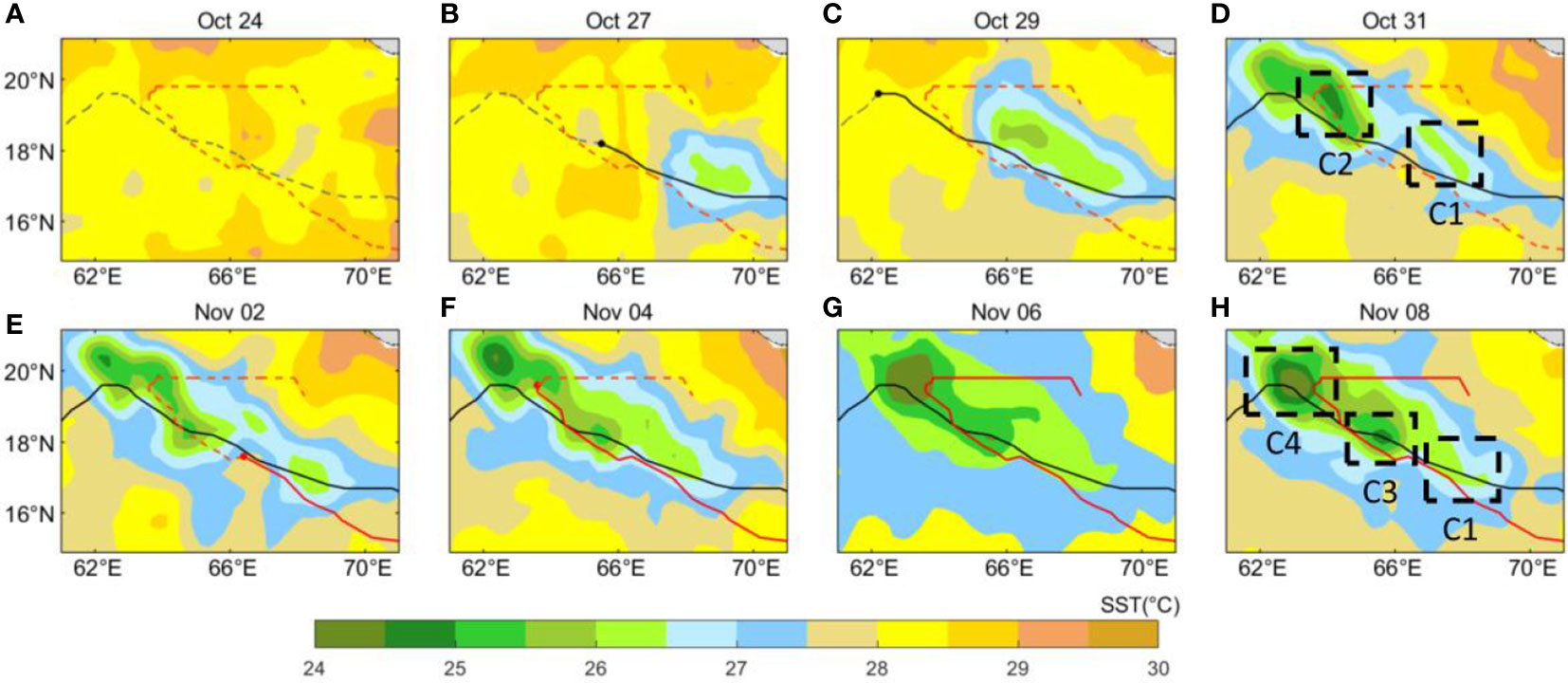
Figure 3 The tracks of TCs Kyarr (A) and Maha (B) were provided by JTWC, ERA5 and WRF model simulation, respectively.

FIGURE 4

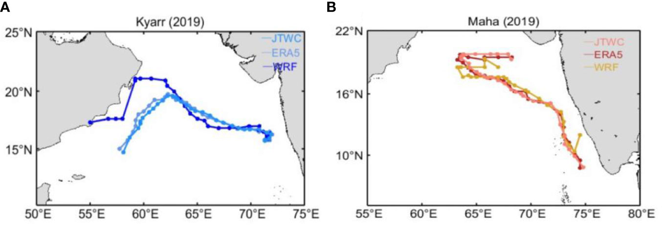
Figure 4 Evolution of the SST before, during and after Kyarr and Maha. (A): before Kyarr, (B, C): during Kyarr, (D): after Kyarr and before Maha, and (E–H): after Kyarr and during Maha. The black and red lines denote the tracks of Kyarr and Maha, respectively. The grey and red dotted lines represent that the TCs have not passed through the regions. The black and red solid dots denote the centre locations of Kyarr and Maha at 00:00 UTC, respectively. The black boxes represent typical regions with distinct sea surface cooling.

As seen in Figures 3E–H, the sea surface cooled again after the Maha passed through the same area 8 days later (Figure 3H). And two more new cooling patches emerged, regions C3 and C4, their temperature decreases of 5°C and 4.5°C, respectively. While the first cooling patch in region C1 continued to enlarge, the maximum SST drop in region C2 gradually recovered during the passage of TC Maha (Figures 3E–H). Thus, after the passage of Kyarr and Maha, there were three cooling regions on the sea surface. And the cooling in region C4 is significantly stronger than that in other regions.

4.4. Horizontal distribution of the wind stress curls

Figure 5 shows the wind field simulated by the WRF model. The calculated wind stress curls were obtained from WRF model simulation and ERA5, respectively. A positive wind stress curl closely linked to Ekman pumping to generate upwelling and promote cold wake development (Chiang et al., 2011). The wind stress curls obtained by WRF model simulation and ERA5 calculation were all positive over the AS, but the wind stress curls according to ERA5 were relatively weak. The ERA5 spatial pattern of the wind stress curls were similar to that of WRF model simulation (Figures 5A–C, G–I), the magnitude was 2–6 times larger for WRF model simulation (Figures 5D–F, I, J). For example, at 00:00 UTC on October 27, the wind stress curls of Kyarr obtained from WRF model simulation were obviously four times stronger than that of ERA5. The maximum value of the wind stress curls from ERA5 was ~1.1×10^-5 N/m³ (Figure 5A) and that from WRF model simulation was~5×10^-5 N/m³ (Figure 5D). The maximum value of wind stress curls of Maha obtained from ERA5 was ~0.8×10^-5 N/m³ (Figure 5I) and that from WRF model simulation was ~4.8×10^-5 N/m³ (Figure 5L), at 18:00 UTC on November 04. The powerful wind of the TCs induced a series of physical processes, and the sea surface cooled, as shown in Figure 3. As the SST decreased along the TC tracks analyzed above, it can be seen that the wind forcing according to ERA5 was too weak to produce this feature. In contrast, the WRF-obtained atmospheric forcing could produce this cold wake more realistically.

4.5. Chlorophyll a concentration corresponding to the two sequential tropical cyclones

Figure 6 shows the time evolution of chl-a concentration at sea surface caused by Kyarr and Maha. The chl-a concentration was 0.5~1 mg/m³ in most areas of AS before two sequential TCs (Figure 6A). Unsurprisingly, the three typical regions with obvious sea surface cooling and affected by strong wind stress curls were also noted to exhibit pronounced increases in chl-a after two sequential TCs. During the passage of TC Kyarr, the chl-a concentration did not significantly increase along the TC track but showed only a small increase of 2 mg/m³ near the generation region of Kyarr (Figure 6B). After Kyarr and during Maha, there were three chl-a concentration regions: the region near the generation of Kyarr and regions C1 and C3. In these three regions, the chl-a concentration could reach ≥ 3.5 mg/m³ (Figure 6C). After the passage of Kyarr and Maha, the chl-a concentration in the region near the generation of Kyarr did not obviously increase. In region C1, the chl-a concentration gradually returned to ≤ 2.5 mg/m³. In region C3, the chl-a concentration increased to a maximum of 4.5 mg/m³, and another chl-a concentration region appeared, region C4. There was a significant increase in the chl-a concentration in this region, with a maximum value > 5 mg/m³.

FIGURE 5

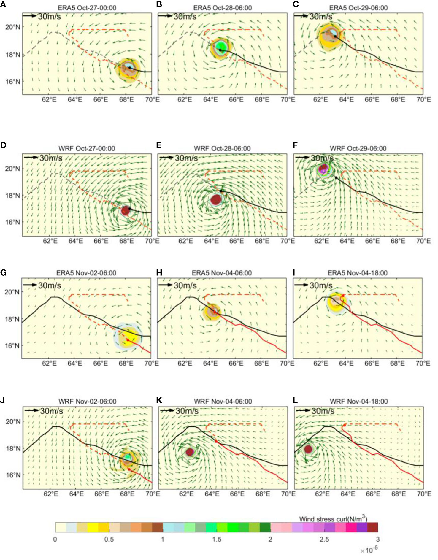
Figure 5 The hourly wind field (arrows: m/s) at 10 m above the sea surface and estimated wind stress curls (colours: N/m³) during (A–F) Kyarr’s passage and (G–L) Maha’s passage from ERA5 data and WRF model simulation, respectively. The expression of the TC tracks is the same as that in Figure 3.

4.6. Three cold eddies after the passage of the two sequential tropical cyclones

In Figures 7A–F, the evolution of sea surface relative vorticity is shown. After TC Kyarr passed (Figures 7A–C), the three regions exhibited positive relative vorticity, regions C1, C3, and C4 reached approximately 1×10^-5 s^-1, 1.5×10^-5 s^-1, and 1×10^-5 s^-1, respectively. Interestingly, after TC Kyarr passed through, a positive relative vorticity also appeared in between of regions C3 and C4 (Figure 7C). However, the relative vorticity in this region was smaller than the relative vorticity in regions C3 and C4 and gradually weakened (Figures 7D–F). After Maha passed, the positive relative vorticity of regions C3 and C4 developed further and reached maximum values of 2×10^-5 s^-1 and 3×10^-5 s^-1, respectively. The relative vorticity of region C1 did not change significantly, but the area with positive relative vorticity in this region increased (Figures 7D–F). Because cyclonic eddies are closely linked to the positive relative vorticity, further research on this topic is presented in the next section.

FIGURE 6

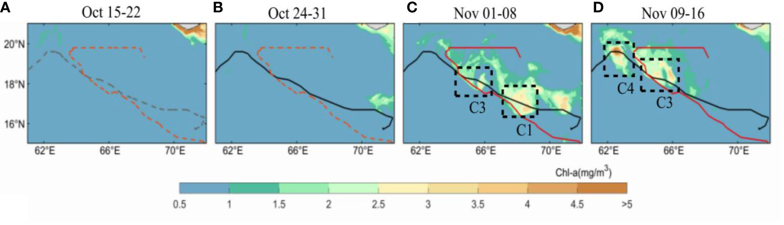
Figure 6 Observations of the 8-day mean chl-a concentration (mg/m³ ) before, during and after Kyarr and Maha. (A): before Kyarr, (B): during Kyarr, (C): after Kyarr and during Maha, and (D): after Kyarr and Maha. The expression of the TC tracks is the same as that in Figure 4. The black boxes represent three typical regions with obvious chl-a increases and sea surface cooling, as shown in Figure 4.

FIGURE 7

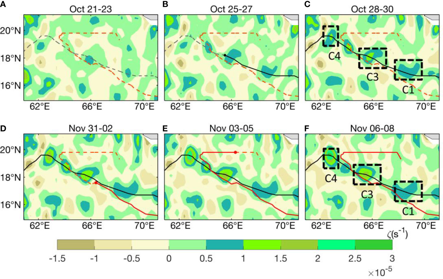
Figure 7 The calculated 3-day mean sea surface relative vorticity (colours: s^-1 ) before, during and after the passage of Kyarr and Maha. (A): before Kyarr, (B, C): during Kyarr, (D, E): after Kyarr and during Maha, and (F): after Kyarr and Maha. The expression of the TC tracks is the same as that in Figure 3. The black boxes represent three typical regions with obvious sea surface relative vorticity increases and sea surface cooling, as shown in Figure 3.

Figure 8 depicts the temporal evolution of the SSHA before, during and after the passage of Kyarr and Maha. At first, no SSHA existed before the two sequential TCs (Figure 8A). Then a SSHA began to appear during the passage of TC Kyarr(Figure 8B). Meanwhile, a cold eddy was first identified by eddy detection algorithms in the area during the passage of TC Kyarr (Figure 8B). Then, as Kyarr continued to advance, a second SSHA appeared on the sea surface. And a second cold eddy was also identified (Figure 8C). After the passage of Kyarr, the sea surface height in C1, C3 and C4 regions decreased by -10 cm, -15 cm and -15 cm, respectively. And a third cold eddy was identified at location of the turn in Kyarr’s track (Figure 8D). In the three cold eddy areas, the sea surface geostrophic currents gradually strengthened and showed the characteristics of cyclone (Figures 8B–D). Moreover, during the passage of Maha, negative SSHAs were further reinforced. In region C1, the sea surface height decreased by approximately -15 cm. In regions C3 and C4, the sea surface height extensively decreased, and both reached -25 cm. The sea surface geostrophic currents formed more intense cyclonic features in these regions, and the highest velocities were found around the edges of the three cold eddies (Figures 8E, F). Finally, the shape of the three cold eddies stabilized on November 07 (Figure 7F).

FIGURE 8

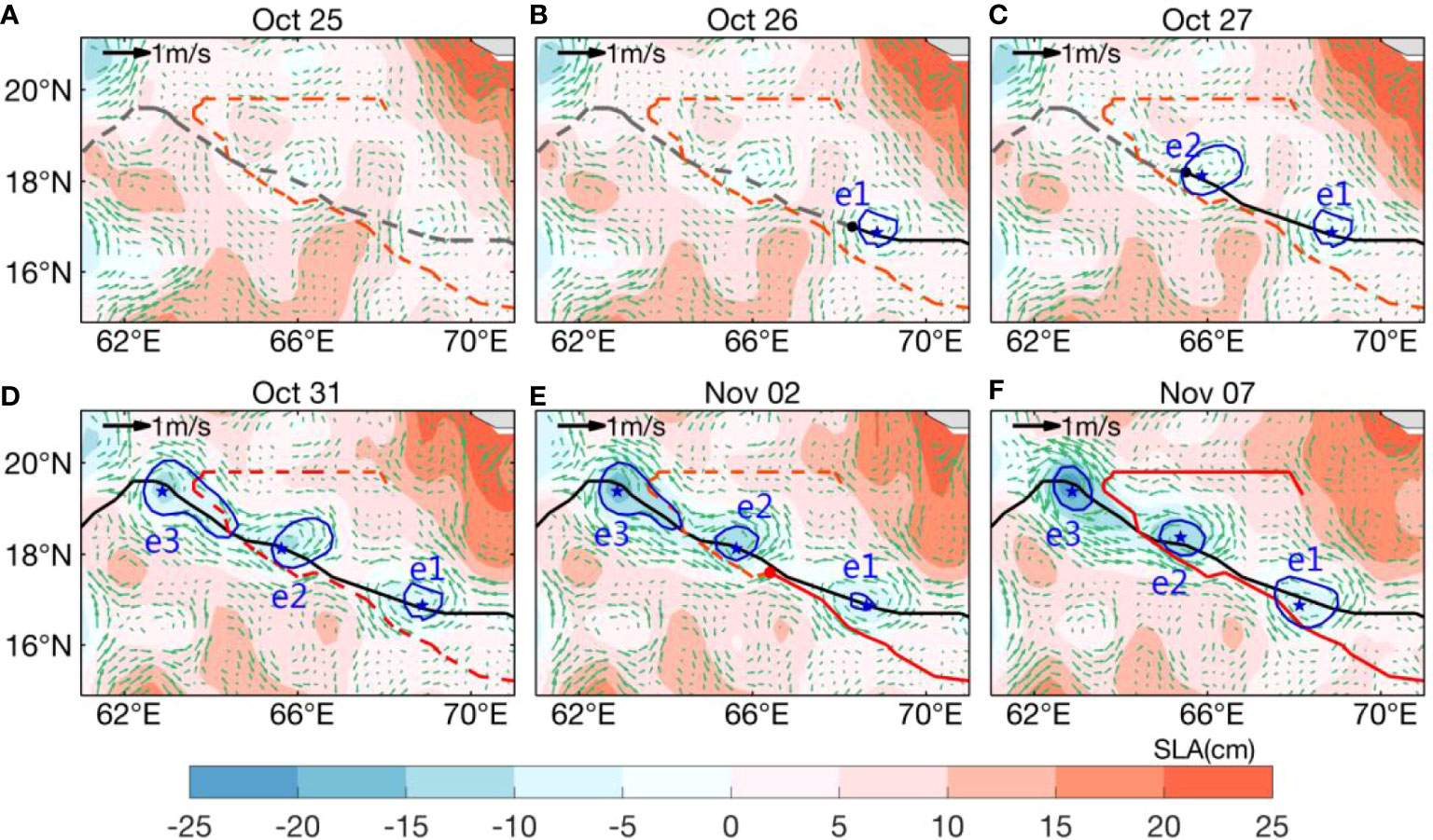
Figure 8 Observations of SSHAs (colours: cm) and geostrophic velocity of zonal/meridional components (arrows: m/s) before , during and after the passage of the two TCs. (A): before Kyarr, (B, C): during Kyarr, (D): after Kyarr and before Maha, and (E): after Kyarr and during Maha. (F): after Kyarr and Maha. The solid blue lines show the shape of eddies, and the blue five-pointed stars show the centre of the eddies. The expression of the TC tracks is the same as that in Figure 3. The black boxes represent three typical regions with obvious SSHA decreases and sea surface cooling, as shown in Figure 3.

After the two TCs passed through on November 07, three stable cold eddies were identified by eddy detection algorithms. The centre of cyclonic eddy e1 in region C1 was located at 68.125°E, 16.875°N and had a radius of up to 69 km and an area of up to ~15000 km². The centre of cyclonic eddy e2 was located at 65.375°E, 18.375°N and had a radius of up to 50 km and an area of up to ~7850 km². The centre of cyclonic eddy e3 was located at 68.125°E, 16.875°N and had a radius of up to 41 km and an area of up to ~5280 km². Each eddy radius is defined as the average distance between the eddy boundary and the centre of the eddy identified by the eddy detection algorithms. The long forcing time of strong wind during the passage of Kyarr and Maha are shown in Table 2. The maximum forcing time of each eddy was all much longer than the geostrophic adjustment time during the passage of Kyarr. However, during the passage of Maha, the maximum forcing time was all slightly below the maximum adjustment time in these three cold eddy regions.

TABLE 2

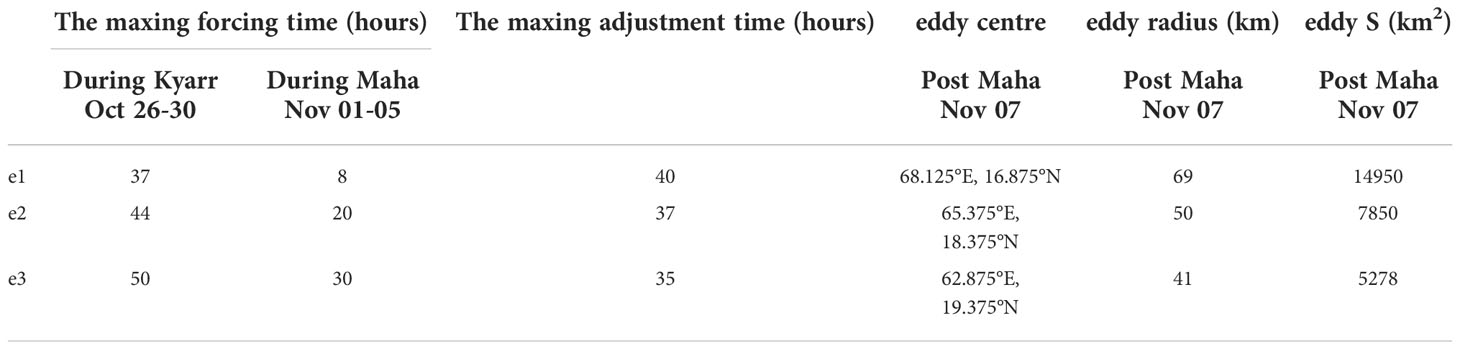
Table 2 Information about cyclonic eddies identified by eddy detection algorithms.

4.7. Temperature structure and the depth integrated heat content of the upper ocean

Figures 2A–E show the variations in temperature profiles from five Argo floats. Figure 2F shows the temporal and spatial variations in the five selected Argo floats. According to Figure 2F, Argo floats were located near the tracks of Kyarr and Maha. And Argo floats 2902202, 2902205, and 2902272 were concentrated near e1. Argo float 2902175 was somewhat far from e1, approximately 100 km from the edge of e1, and Argo float 2902210 was located approximately 50 km from the edge of e2. The five Argo floats recorded changes in the ocean at different times during the passage of Kyarr and Maha. For example, Argo floats 29002210 and 2902272 recorded changes in the interior of the ocean caused by TC Kyarr, and Argo floats 2902205, 2902202, and 2902175 recorded changes in the interior of the ocean caused by TC Maha.

Furthermore, similar to the Argo float observations, the spatial series of the HYCOM model output results were added to the temperature profile to demonstrate that HYCOM model can reproduce ocean conditions. However, the upper ocean temperature changes captured by the HYCOM model output after the passage of TC Kyarr were more affected than the temperature changes recorded by Argo floats, and the temperature decreased even more dramatically (Figures 2A–E). In general, the HYCOM model output results were generally consistent with the Argo float measurements.

In this study, the upper ocean is defined as depths of 0–200 m. To investigate the thermal response of the upper ocean, the heat content change (ΔH ) was calculated from a pair of temperature profiles from each Argo float (Zedler et al., 2002).

$\begin{array}{ll}\Delta H=\rho 0Cpw{\displaystyle \underset{200}{\overset{0}{\int }}\Delta T(z)dz}& (9)\end{array}$

Here, ρ0 is the density of seawater, and Cpw is the specific heat of seawater, so ρ0Cpw = 4.1 MJ°C^-1 m^-3. Integration is performed over depths of 0 to 200 m. ΔT is the change in sea water temperature before and after the TCs, as shown in Figure 2 for the Argo float temperature profile of the time series. A negative value indicates heat loss and a positive value indicates heat gain within a specified depth range. As shown in Figure 9, the ΔH calculated from the Argo profiles demonstrated a significant difference.

FIGURE 9

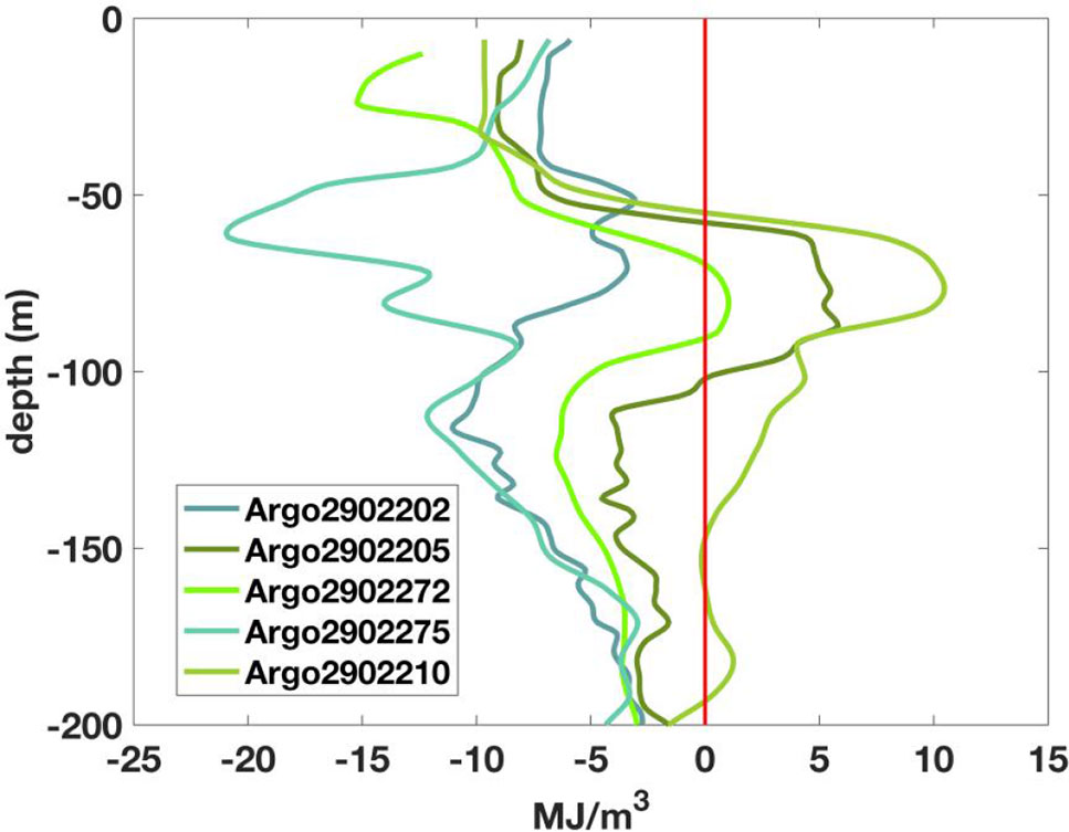
Figure 9 Vertical profiles of the heat content anomaly according to each Argo float.

Argo floats 2902175 and 2902202 showed that the upper 200 m of the ocean lost heat along the temperature profiles, while Argo floats 2902210, 2902205, and 2902272 showed that heat was gained in the subsurface ocean (50-100 m). And Argo float 2902210 showed that a subsurface ocean heat increase could reach 13 MJ°C^-1 m^-3, Argo float 2902205 showed a subsurface ocean heat increase of approximately 6 MJ°C^-1 m^-3. Argo float 2902272 showed a subsurface ocean heat increase of 2 MJ°C^-1 m^-3. Moreover, Argo float 2902210 showed an ocean heat gain of approximately 180 m. In previous sections, it was found that the passage of Kyarr led to the generation of three cold eddies. The interior of the cold eddy is an unstable thermal structure. Therefore, the heat flux exchanges inside cold eddies need to be further studied.

4.8. Nondimensionalization of the two sequential tropical cyclones

Some of the nondimensional numbers defined in previous studies help to reveal the characteristics of TCs and their interactions with the upper ocean. The external parameters that characterize the ocean environments and the two sequential TCs are exhibited and listed in Table 3. The calculation results for each TC are presented in Table 4. For each TC, the nondimensional storm speed S is O(1), where S is the ratio of the local inertial period to the TC residence time (Price et al., 1994). The strong wind stresses of TCs caused changes in the interior of the ocean that were basically consistent with the local inertial period. The Burger number B reveals the degree of pressure coupling between the mixed-layer currents and the thermocline currents (Price et al., 1994). For each TC case, a relatively large Burger number can be seen, and it is expected that the pressure coupling is very pronounced during the TC passage. The translation speeds of TCs Kyarr and Maha were only slightly greater than c (the gravest mode internal wave). Each TC had an O(1) Mach number. Previous studies have shown that under these conditions, significant upwelling occurs directly beneath TCs (Price et al., 1994). And it was caused by Ekman pumping, which is closely linked to positive wind stress curls (Figure 5). Therefore, the calculations of these nondimensional numbers for each TC case show that two slow and strong TCs have considerable impacts on the upper ocean interior during their passage (Price et al., 1994).

TABLE 3

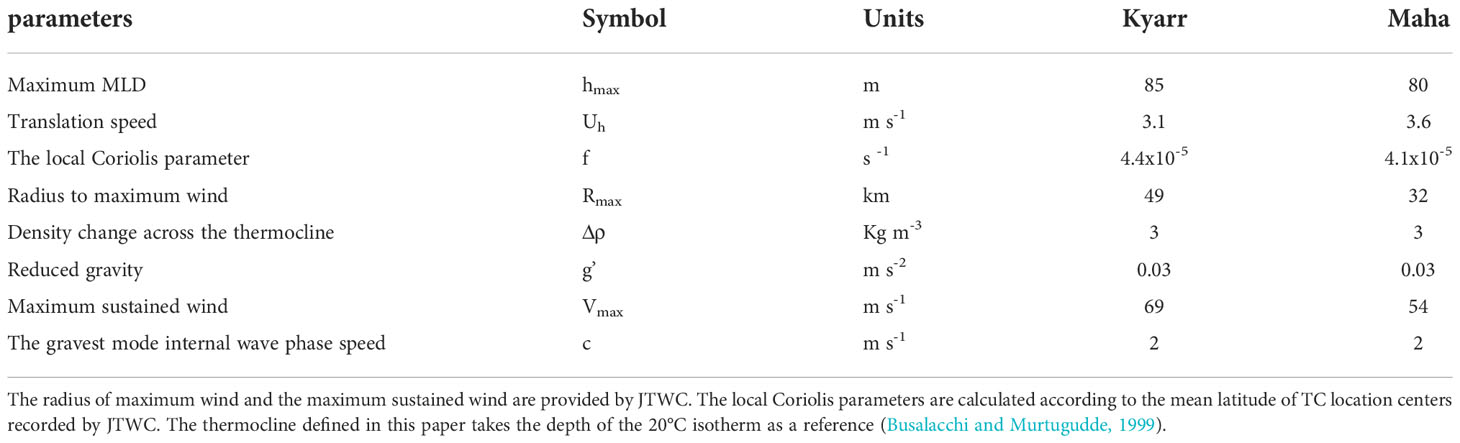
Table 3 External parameters.

TABLE 4

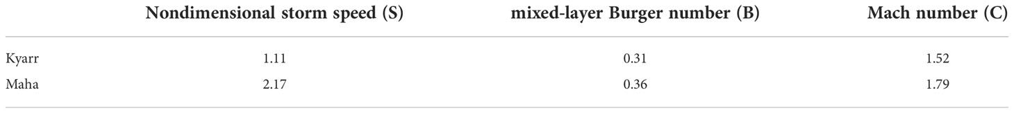
Table 4 Nondimensional variables.

Figures 10A–C show the changes in vertical temperature profiles and the depth of mixed-layers before, during and after Kyarr and Maha in the upper ocean at the three cyclonic eddy centres. At each eddy centre, the initial MLD was approximately 40 m, and the MLT was approximately 29°C. Then, the MLT and MLD changed sharply due to the influence of the passage of TCs. The cooling of the MLT was accompanied by the deepening of the MLD; the MLT decreased by at least 3°C, and the MLD deepened to at least 55 m at each eddy centre after Kyarr passed. For example, after the passage of Kyarr, the MLT in the central area of e2 decreased the most sharply, by approximately 5°C (Figure 10B), the MLD deepened by approximately 75 m. After the passage of Kyarr in e3, the MLD deepened the most, up to 80 m, and the MLT dropped to approximately 26°C (Figure 10C). After Maha passed through the three cold eddies, it also caused the MLD in each eddy centre to deepen and the MLT to decrease, but none of the changes were as pronounced as those after Kyarr passed through. The differences in the variations in MLD and MLT at the e1, e2, and e3 centres were mainly due to the different characteristics of each TC when they were passing these cold eddy fields. Based on the nondimensional characteristics of each TC calculated in section 4.8, two slow-moving TCs can cause strong vertical mixing and upwelling, causing the cooling of the MLT and deepening the MLD. What’s more, the sea water temperature at 150-200 m remained virtually unchanged during the whole period.

FIGURE 10

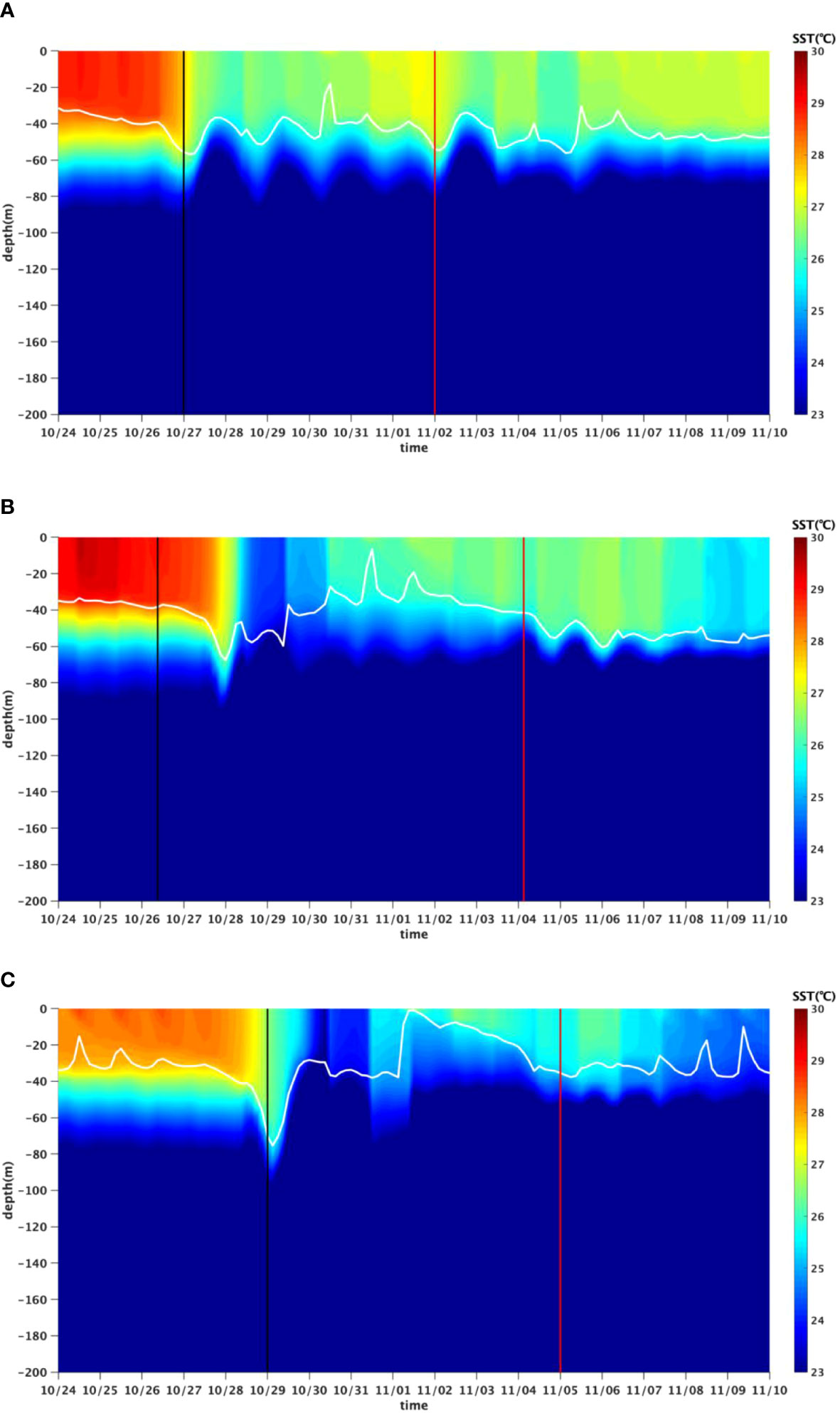
Figure 10 Vertical profiles of temperature in the central range of each eddy over time. (A): Vertical profiles of temperature in the central range of e1 over time. (B): Vertical profiles of temperature in the central range of e2 over time. (C): Vertical profiles of temperature in the central range of e3 over time. The solid white lines indicate the depth of each eddy centre mixed-layer. The black and red solid lines denote the times when Kyarr and Maha passed by each eddy, respectively.

The passage of TCs greatly influenced the depth integrated heat (DIH) content of the upper ocean. Figures 10A–C show the temperature profiles of each eddy centre. The maximum temperature in each eddy centre response to each TC occurred approximately 48 h after the TCs passed. Therefore, T0(z) was the 24-h average during the temperature response to TCs at each eddy centre before the TCs (on October 24). And T1(z) was the 48-h average during the temperature response to TCs at each eddy centre after the TCs. The DIH anomaly could be obtained from the temperature profiles by integrating the temperature anomaly (T1(z)–T0(z)) over an appropriate depth range and multiplying it by the density and specific heat of sea water. Thus, following Zedler (Zedler, 2002), the computation of the DIH anomaly is as follows:

$\begin{array}{ll}DIH=\rho 0Cpw{\displaystyle \underset{Z1}{\overset{Z0}{\int }}(T1(Z)-T0(Z))dZ}& (10)\end{array}$

Integration was performed over depths of z1 to z2 (z is positive downwards). To examine the separate contributions between different layers of the upper ocean, three depth ranges were chosen for integration: a shallow depth range as the MLD, a middle layer that was the MLD bottom to the 150 m depth, and a bottom layer that was the 150 m to 200 m depth. The shallow range effectively quantified the MLD cooling occurring after the passage of TCs and was therefore denoted DIH_ML; the middle layer was denoted DIH_MD, and the bottom layer was denoted DIH₂₀₀.

The depth ranges and the corresponding DIH values of each eddy centre for the TCs are summarized in Table 5. The two TCs were associated with heat loss from the three different layers, but the largest loss occurred in the middle layer after Maha, where DIH_ML = -1220.0 MJ m^-2 in the e1 eddy centre, and another large middle layer heat loss in the Maha case similar to that observed for the e1 eddy centre occurred when DIH_ML = -1192.3 MJ m^-2 over the depth range [53 m, 150 m]. These different DIH values may be partly due to the difference in vertical mixing and upwelling intensity in the upper ocean caused by TCs Kyarr and maha as they passed through the central region of each cold eddy.

TABLE 5

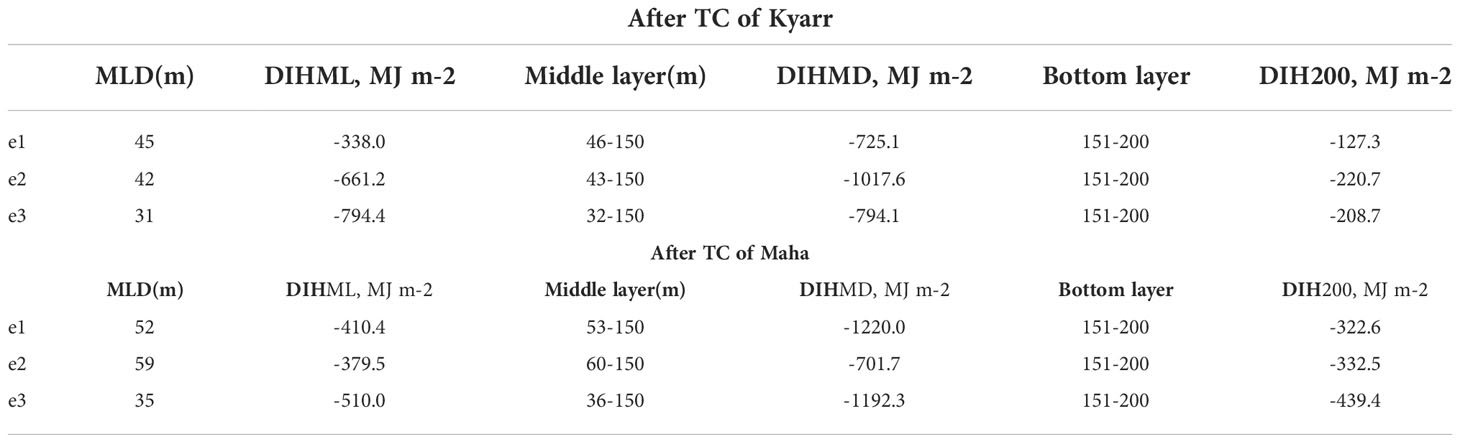
Table 5 Depth integrated heat anomaly.

5. Conclusion

The response of the upper ocean to Kyarr and Maha, including the generation mechanism of cold eddies and heat flux exchanges in the eddy centre fields, is discussed in this study by using satellite data, numerical model outputs,in situ observations.

The two sequential TCs followed a similar path, with a slow translation speed over the same area in the AS from October 24 to November 06, 2019. During the passage of Kyarr and Maha, the SST significantly decreased in three regions due to strong ocean vertical mixing and upwelling. The wind field data provided by the WRF model simulation and ERA5 were compared. Wind stress curls were thus calculated. The WRF model simulation could better reproduce the TC wind field and better match the SST reduction magnitude. Meanwhile, the sea surface chl-a concentration was enhanced by Kyarr and Maha. The regions with particularly pronounced chl-a enhancement coincided well with sea surface cooling regions. More importantly, based on the use of eddy detection algorithms, three cold eddies with negative SSHAs were found along the track of Kyarr. In general, the long forcing time of strong positive wind stress curls has mainly contributed to the generation of the three cyclonic cold eddies during the passage of two sequential TCs. Positive wind stress curls can produce upwelling due to Ekman responses. What’s more, along with the injection of positive relative vorticity, the sea surface presents cyclonic changes.

Moreover, obvious thermodynamic responses in the upper ocean occurred at each eddy field interior. During the passage of Kyarr and Maha, the TCs had superimposed effects on the upper ocean and caused strong vertical mixing and upwelling. And the upwelling was enhanced by the instability of thermal structure inside the cold eddy (eddy-wind Ekman pumping and eddy pumping).

The variation in heat content (ΔH ) was calculated from the temperature distribution of five Argo floats. Three Argo floats, located near e1(2902272, 2902205) and e2(2902010), showed subsurface warming and increased heat. Moreover, the Argo float (2902010) showed heat gain in the bottom layer.

In order to further study the heat flux exchanges in the upper ocean in the central region of each cold eddy. Specific heat flux exchanges between different layers of the upper ocean were studied by using HYCOM model output results. The upper 200 m of each eddy centre field was divided into three layers: the mixed-layer, the middle layer and the bottom layer. The DIH of the three layers in the three cold eddy centre fields were calculated in turn after each TC passed. All three eddy centre fields showed heat loss from different layers after the TCs.

Regardless, strong vertical mixing and upwelling are the main factors that influence eddy centre fields heat flux exchanges, but it is not clear how much of each term contributes to the heat flux exchanges in different layers. Is there a difference between the main time periods of vertical mixing and upwelling?

Therefore, further studies are needed to improve the understanding of the relationship between the two sequential TCs. And their interaction with the upper ocean by combining the coupled ocean numerical model with in situ observations. It can be determined the thermal modulation process inside cold eddies when a TC passes through.

Data availability statement

Publicly available datasets were analyzed in this study. This data can be found here: https://www.ecmwf.int/, https://psl.noaa.gov/data/gridded/data.ncep.reanalysis.derived.surface.html/, http://marine.copernicus.eu/, ftp://ftp.ifremer.fr/ifremer/argo, https://www.hycom.org/.

Author contributions

ZS: completed the whole article research content and wrote the manuscript. SZ: instructed the first author to complete the whole paper. All authors contributed to the article and approved the submitted version.

Funding

This work was supported by the National Natural Science Foundation of China (92158201, 41876005), the Innovation and Entrepreneurship Project of Shantou (2021112176541391), and the Scientific Research Start-Up Foundation of Shantou University (NTF20006).

Conflict of interest

The authors declare that the research was conducted in the absence of any commercial or financial relationships that could be construed as a potential conflict of interest.

Publisher’s note

All claims expressed in this article are solely those of the authors and do not necessarily represent those of their affiliated organizations, or those of the publisher, the editors and the reviewers. Any product that may be evaluated in this article, or claim that may be made by its manufacturer, is not guaranteed or endorsed by the publisher.

References

Babin S. M., Carton J. A., Dickey T. D., Wiggert J. D. (2004). Satellite evidence of hurricane-induced phytoplankton blooms in an oceanic desert. J. Geophysical Research-Oceans 109 (C3). doi: 10.1029/2003JC001938

CrossRef Full Text | Google Scholar

Busalacchi A., Murtugudde R. (1999). Interannual variability of the dynamics and thermodynamics of the tropical Indian ocean. J. Climate 12, 2300–2326. doi: 10.1175/1520-0442(1999)012%3C2300:IVOTDA%3E2.0.CO;2

CrossRef Full Text | Google Scholar

Chassignet E. P., Hurlburt H. E., Smedstad O. M., Halliwell G. R., Hogan P. J., Wallcraft A. J., et al. (2007). The HYCOM (HYbrid coordinate ocean model) data assimilative system. J. Mar. Syst. 65 (1-4), 60–83. doi: 10.1016/j.jmarsys.2005.09.016

CrossRef Full Text | Google Scholar

Cheng W., Steenburgh W. J. (2005). Evaluation of surface sensible weather forecasts by the WRF and the eta models over the western united states. Weather Forecasting 20 (5), 812–821. doi: 10.1175/WAF885.1

CrossRef Full Text | Google Scholar

Cheng L., Zhu J., Sriver R. L. (2015). Global representation of tropical cyclone-induced short-term ocean thermal changes using argo data. Ocean Sci. 11 (5), 719–741. doi: 10.5194/os-11-719-2015

CrossRef Full Text | Google Scholar

Chiang T. L., Wu C. R., Oey L. Y. (2011). Typhoon kai-tak: An ocean’s perfect storm. J. Phys. Oceanography 41, 221–233. doi: 10.1175/2010JPO4518.1

CrossRef Full Text | Google Scholar

Davis C., Wang W., Chen S. S., Chen Y. S., Corbosiero K., DeMaria M., et al. (2008). Prediction of landfalling hurricanes with the advanced hurricane WRF model. Monthly Weather Rev. 136 (6), 1990–2005. doi: 10.1175/2007MWR2085.1

CrossRef Full Text | Google Scholar

Evan A. T., Camargo S. J. (2011). A climatology of Arabian Sea cyclonic storms. J. Climate 24 (1), 140–158. doi: 10.1175/2010JCLI3611.1

CrossRef Full Text | Google Scholar

Gill A. E., Green J., Simmons A. J. (1974). Energy partition in the large-scale ocean circulation and the production of mid-ocean eddies. Deep Sea Res. Oceanographic Abstracts 21 (7), 499, N1508–509, N1, 528. doi: 10.1016/0011-7471(74)90010-2

CrossRef Full Text | Google Scholar

Gilson J., Roemmich D. (2001). Eddy transport of heat and thermocline waters in the north pacific: A key to interannual/decadal climate variability? J. Phys. Oceanography 21, 675–687. doi: 10.1175/1520-0485(2001)031<0675:ETOHAT>2.0.CO;2

CrossRef Full Text | Google Scholar

Hu J. Y., Kawamura H. (2004). Detection of cyclonic eddy generated by looping tropical cyclone in the northern south China Sea: a case study. Acta Oceanologica Sin. 23 (2), 213–224.

Google Scholar

Jaimes B., Shay L. K. (2009). Mixed-layer cooling in mesoscale oceanic eddies during hurricanes Katrina and Rita. Monthly Weather Rev. 137 (12), 4188–4207. doi: 10.1175/2009MWR2849.1

CrossRef Full Text | Google Scholar

Kara A. B., Rochford P. A., Hurlburt H. E. (2000). An optimal definition for ocean mixed-layer depth. J. Geophysical Research: Oceans 105 (C7), 16803–16821. doi: 10.1029/2000JC900072

CrossRef Full Text | Google Scholar

Lu Z. M., Wang G. H., Shang X. D. (2016). Response of a preexisting cyclonic ocean eddy to a typhoon. J. Phys. Oceanography 46 (8), 2403–2410. doi: 10.1175/JPO-D-16-0040.1

CrossRef Full Text | Google Scholar

Lu Z. M., Wang G. H., Shang X. D. (2020). Strength and spatial structure of the perturbation induced by a tropical cyclone to the underlying eddies. J. Geophysical Research-Oceans 125 (5). doi: 10.1029/2020JC016097

CrossRef Full Text | Google Scholar

Mayer D. A., Mofjeld H. O., Leaman K. D. (1981). Near-inertial internal waves observed on the outer shelf in the middle Atlantic bight in the wake of hurricane belle. J. Phys. Oceanograph. 11 (1), 87–106. doi: 10.1175/1520-0485(1981)011%3C0087:NIIWOO%3E2.0.CO;2

CrossRef Full Text | Google Scholar

Mohapatra M., Srivastava A. K., Balachandran S., Geetha B. (2017). Inter-annual variation and trends in tropical cyclones and monsoon depressions over the north Indian ocean (Springer Singapore) 89–106. doi: 10.1007/978-981-10-2531-0_6

CrossRef Full Text | Google Scholar

Nencioli F., Dong C. M., Dickey T., Washburn L., McWilliams J. C. (2010). A vector geometry-based eddy detection algorithm and its application to a high-resolution numerical model product and high-frequency radar surface velocities in the southern California bight. J. Atmospheric Oceanic Technol. 27 (3), 564–579. doi: 10.1175/2009JTECHO725.1

CrossRef Full Text | Google Scholar

Okubo A. (1970). Horizontal dispersion of floatable particles in vicinity of velocity singularities such as convergences. Deep Sea Res. Oceanographic Abstracts 17 (3), 445–454. doi: 10.1016/0011-7471(70)90059-8

CrossRef Full Text | Google Scholar

Osuri K. K., Mohanty U. C., Routray A., Kulkarni M. A., Mohapatra M. (2012). Customization of WRF-ARW model with physical parameterization schemes for the simulation of tropical cyclones over north Indian ocean. Natural Hazards 63 (3), 1337–1359. doi: 10.1007/s11069-011-9862-0

CrossRef Full Text | Google Scholar

Park J.-H., Yeo D.-E., Lee K. J., Lee H., Lee S.-W., Noh S., et al. (2019). Rapid decay of slowly moving typhoon soulik, (2018) due to interactions with the strongly stratified northern East China Sea. Geophysical Res. Lett. 46 (24), 14595–14603. doi: 10.1029/2019GL086274

CrossRef Full Text | Google Scholar

Potter H., Drennan W. M., Graber H. C. (2017). Upper ocean cooling and air-sea fluxes under typhoons: A case study. J. Geophysical Research-Oceans 122 (9), 7237–7252. doi: 10.1002/2017JC012954

CrossRef Full Text | Google Scholar

Powell M. D., Vickery P. J., Reinhold T. A. (2003). Reduced drag coefficient for high wind speed in tropical cyclones. Nature 422 (6929), 279–283. doi: 10.1038/nature01481

PubMed Abstract | CrossRef Full Text | Google Scholar

Prasad T. G., Hogan P. J. (2007). Upper-ocean response to hurricane Ivan in a 1/25° nested gulf of Mexico HYCOM. J. Geophysical Res 112. doi: 10.1029/2006JC003695

CrossRef Full Text | Google Scholar

Price J. F., Sanford T. B., Forristall G. Z. (1994). Forced stage response to a moving hurricane. J.phys.oceanogr 24 (2), 233–260. doi: 10.1175/1520-0485(1994)024%3C0233:FSRTAM%3E2.0.CO;2

CrossRef Full Text | Google Scholar

Qiu B., Chen S. (2005). Eddy-induced heat transport in the subtropical north pacific from argo, TMI, and altimetry measurements. J. Phys. oceanography 35, 458–473. doi: 10.1175/JPO2696.1

CrossRef Full Text | Google Scholar

Qiu C. H., Liang H., Sun X. J., Mao H. B., Wang D. X., Yi Z. H., et al. (2021). Extreme Sea-surface cooling induced by eddy heat advection during tropical cyclone in the north Western pacific ocean. Front. Mar. Sci. 8. doi: 10.3389/fmars.2021.726306

CrossRef Full Text | Google Scholar

Sun L., Yang Y., Xian T., Lu Z., Fu Y. (2010). Strong enhancement of chlorophyll a concentration by a weak typhoon. Mar. Ecol. Prog. Ser. 404, 39–50. doi: 10.3354/meps08477

CrossRef Full Text | Google Scholar

Tsai Y., Chern C. S., Wang J. (2008). The upper ocean response to a moving typhoon. J. Oceanogr 64, 115–130. doi: 10.1007/s10872-008-0009-1

CrossRef Full Text | Google Scholar

Wang L., Lau K. H., Fung C. H., Gan J. P. (2007). The relative vorticity of ocean surface winds from the QuikSCAT satellite and its effects on the geneses of tropical cyclones in the south China Sea. Tellus Ser. A-Dynamic Meteorology Oceanography 59 (4), 562–569. doi: 10.1111/j.1600-0870.2007.00249.x

CrossRef Full Text | Google Scholar

Yang Y. J., Sun L., Duan A. M., Li Y. B., Fu Y. F., Yan Y. F., et al. (2012). Impacts of the binary typhoons on upper ocean environments in November 2007. J. Appl. Remote Sens. 6 (1), 3583. doi: 10.1117/1.JRS.6.063583

CrossRef Full Text | Google Scholar

Yang G., Yu W. D., Yuan Y. L., Zhao X., Wang F., Chen G. X., et al. (2015). Characteristics, vertical structures, and heat/salt transports of mesoscale eddies in the southeastern tropical Indian ocean. J. Geophysical Research-Oceans 120 (10), 6733–6750. doi: 10.1002/2015JC011130

CrossRef Full Text | Google Scholar

Zedler S. E., Dickey T. D., Doney S. C., Price J. F., Yu X., Mellor G. L., et al. (2002). Analyses and simulations of the upper ocean's response to hurricane Felix at the Bermuda testbed mooring site: 13–23 august 1995. J. Geophysical Research: Oceans 107, 251–2529. doi: 10.1029/2001JC000969

CrossRef Full Text | Google Scholar

Zhang Y. C., Chen X., Dong C. M. (2019). Anatomy of a cyclonic eddy in the kuroshio extension based on high-resolution observations. Atmosphere 10 (9). doi: 10.3390/atmos10090553

CrossRef Full Text | Google Scholar

Zhang H., Chen D., Zhou L., Liu X. H., Ding T., et al. (2016). Upper ocean response to typhoon kalmaegi, (2014). J. Geophysical Research-Oceans 121 (8), 6520–6535. doi: 10.1002/2016JC012064

CrossRef Full Text | Google Scholar