Acoustic sampling of Antarctic krill with simulated underwater buoyancy gliders: Does the sawtooth dive pattern work?

1. Introduction

Fisheries surveys often use echosounders to measure the distribution, density and shoaling characteristics of marine species (Fernandes et al., 2002; Trenkel et al., 2016). These surveys are traditionally conducted by ships, but experiments with various autonomous underwater platforms (e.g., Fernandes et al., 2000; Greene et al., 2014; Guihen et al., 2014; Benoit-Bird et al., 2018; Lembke et al., 2018; De Robertis et al., 2019) suggest that acoustic measurements collected by alternative samplers may augment or, in some cases, replace ship-based measurements. Autonomous underwater gliders (hereafter gliders) have been recommended as one component of an observation-modeling framework for understanding open ocean ecosystem dynamics (Handegard et al., 2013). Gliders with instrument payloads that include calibrated echosounders suitable for collecting acoustic backscatter data have recently been developed, and the technology continues to improve (Guihen et al., 2014; Guihen, 2018; Benoit-Bird et al., 2018; Chave et al., 2018; Ruckdeschel et al., 2020).

Antarctic krill (Euphausia superba, hereafter krill) provide a critical link between predators and autotrophic producers in the Antarctic marine food web (Croxall et al., 1997; Alonzo et al., 2003; Nicol et al., 2008; Hinke et al., 2017). Krill also support the largest fishery (by tonnage) in the Southern Ocean, with recent annual harvests of about 400,000 tonnes (Croxall and Nicol, 2004; Reid et al., 2004; Nicol et al., 2012; CCAMLR Fishery Report, 2021).The U.S. AMLR Program conducted annual ship-based acoustic surveys during the austral summer around the South Shetland Islands, Antarctica from 1986 through 2011 (e.g., Reiss et al., 2008; Reiss et al., 2017). The goal of these surveys was to estimate the annual biomass of krill within Statistical Subarea 48.1, a management area defined by the Commission for the Conservation of Antarctic Marine Living Resources (CCAMLR) and an important krill fishing area (CCAMLR, 2018). The results of these surveys have been used to assess the status and productivity of krill in the region (Kinzey et al., 2018; Kinzey et al., 2019).

Previous efforts to survey krill with gliders have generally been short (occurring over several days, e.g., Guihen et al., 2014; Guihen, 2018) and highlight the need to design surveys that balance demands for collecting oceanographic data and surveying fisheries resources. In 2018, the Antarctic Marine Living Resources Program of the U.S. National Oceanic and Atmospheric Administration (U. S. AMLR Program) transitioned from ship-based surveys to using gliders to perform acoustic krill surveys. Biomass density estimates for krill over a three month period from acoustically-equipped gliders deployed around the Antarctic Peninsula have been developed and additional field studies are ongoing (Reiss et al., 2021).

Buoyancy gliders sample in an up and down sawtooth pattern, cutting diagonal swaths through the water column. The gliders modeled in this study collect acoustic data while diving but not while resurfacing, sampling the water colum 100 m below the glider as it descends. These simulations represent gliders sampling in this sawtooth pattern through a pelagic population with the statistical properties (e.g., skewness, zero inflation, autocorrelation) obtained in ship surveys to assess whether gliders can provide accurate estimates for the mean and standard deviation (SD) of depth-integrated acoustic densities.

We extracted gridded (100 m horizontal by 5 m vertical), ship-based measurements of krill acoustic backscatter densities collected annually for 10 years by the U.S. AMLR Program in two survey strata and treated these as annual populations of “true” (sensu Dichmont et al., 2006) density values. These statistical populations were then sampled by angled swaths in the sawtooth pattern a glider would follow. We compared annual estimates of depth-integrated krill densities calculated from these simulated glider dives to the depth-integrated densities in the populations being sampled. The simulation modeling was scripted in R (R Core Team, 2022).

This study explores how glider survey design might be optimized to minimize variance while accurately estimating density. It does not address potential hardware or target identification issues (e.g, echosounder calibration with depth, conversion of acoustic target strength to biomass) or krill behavior such as the potential for avoidance (e.g. Guihen et al., 2022). The effectiveness of sawtooth sampling, trade-offs in the precision and bias of density estimates when gliders dove to different maximum depths while sampling a given area and using multiple gliders, are evaluated. While this study is not a substitute for additional field studies of glider sampling we consider it an important step towards evaluating the potential of this technology with its novel sampling pattern to provide density estimates for pelagic species.

2. Material and methods

2.1. Simulated populations (U.S. AMLR ship data)

Ship-based acoustic data were collected from transect lines connecting 25 oceanographic stations off Cape Shirreff and 20 stations in Bransfield Strait during January and February of 2001 through 2011 (excluding 2010; Figure 1). Prevailing weather conditions prevented the ships from surveying all transects in some years, and the total distance covered in each stratum and year ranged from 376.2 to 1582.2 km. The distance covered each year in the Cape Shirreff stratum was nearly twice that in Bransfield Strait (Supplementary Table S1).

FIGURE 1

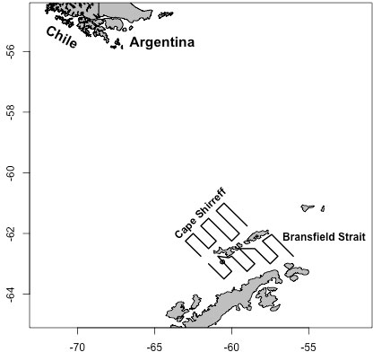
Figure 1 Tracklines for the two U.S. AMLR sampling strata (“Cape Shirreff” and “Bransfield Strait”) around the South Shetland Islands and northern Antarctic Peninsula. Acoustic data sampled by ships following these tracklines were used to define the “true” krill populations in each of ten years for each stratum. These data were subsequently sampled by the simulated gliders.

Echosounders on the ships were calibrated every survey to identify any changes in performance. During acoustic transects, the nominal speed of the vessel was 10 nmi hr^-1 (5.1 m s^-1). Acoustic volume backscattering strength (s_V, dB re 1 m^-1) was collected at 0.5 Hz at three frequencies (38, 120, and 200 kHz) using either a calibrated Simrad EK500 (1996-2004) or a calibrated Simrad EK60 (2005-2011). For this analysis, we extracted the calibrated 120 kHz echosounder data. Acoustic volume densities (s_V) from the surface to 250 m depth were averaged over 5 m vertical by 100 m horizontal bins. Each bin represented approximately 10 acoustic pings. Nautical area scattering coefficients (s_A, m² nmi^-2) were calculated from s_V (MacLennan et al., 2002). A standard three-frequency dB differencing method (Fielding et al., 2012) was applied to distinguish krill from other acoustic targets. Acoustic data from the total distance covered by the ship in each year and stratum were combined into a single “population” representing krill densities at depth for that year and stratum. Thus the two strata over 10 years produced 20 statistical populations for simulated glider sampling.

2.2. Simulated gliders

A single glider sample is one complete descent-ascent cycle, or “dive”. In this simulation, gliders only collect data on the descending portion of the dive but not when ascending. The echosounder is downward facing (facing the seabed perpendicular to the surface during descent). It samples from the surface to 150 m during its angled descent, collecting data to 100 m below the echosounder, so that the maximum depth of acoustic data collection during a dive is 250 m. The gliders do not collect data above the gliders’ location as they descend. This is how many physical gliders have been equipped (Guihen et al., 2014; Guihen, 2018; Chave et al., 2018; Ruckdeschel et al., 2020; Reiss et al., 2021) although gliders with upward facing echosounders (e. g. Benoit-Bird et al., 2018); are also possible. The gliders in current usage by the U.S. AMLR program use either multi-frequency (38kHz; 67.5 kHz and 125 kHZ) or wideband single beam echosounder systems. 100 m range is typical of such systems (Reiss et al., 2021).

Due to a 22.7 degree angle of descent the simulated gliders sample 9 vertical 5 m bins (45 m total) for every horizontal bin (100 m) along their tracklines. A bin is considered fully sampled if the glider sampled any portion of the bin during its descent. Thus, every dive produced a diagonal swath of s_A values from the surface to 250 m (Figure 2) (for illustration purposes the x-axes in Figure 2 are compressed relative to the y-axes).

FIGURE 2

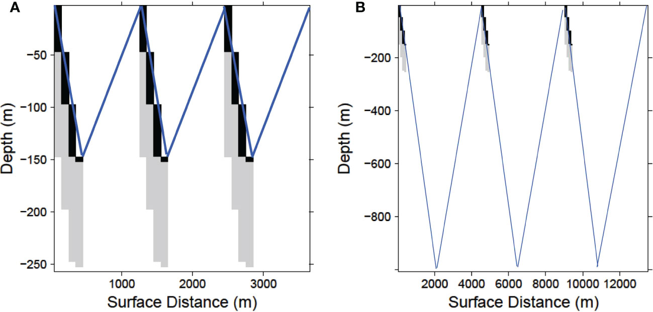
Figure 2 Schematic sample path (not to scale) of a glider completing 3 dives at with a maximum depth of (A) 150 m and (B) 1000 m. In each case the echosounder is shut off at 150 m, but the water column is ensonified 100 m below the glider to a maximum of 250 m as it descends. Black cells indicate when the echosounder is recording which together with the light gray cells represent the sampled area. Blue lines depict the completed glider descent-ascent dives.

Five hundred replicated samples for each maximum dive depth, stratum and year starting from different randomized surface locations were conducted to evaluate the statistical properties of the sampling scheme. Replicate samples of the same population (an individual stratum and year) were modeled by starting each glider at a random location in the first half of the ship-derived population data and then sampling along a continuous trackline on the descending portion of each dive. One half of the trackline length of the population data available for each year and stratum were sampled in a single replicate of multiple dives, resulting in each replicate glider sampling the same number of bins, but different bins, for each stratum and year.

We calculated the mean and SD of the nautical area scattering coefficient (s_A) from all the dives conducted in a year and stratum for each replicate. For each dive, the mean s_A across all bins sampled at each depth (1 to 3 bins for each 5 m depth, Figure 2) was calculated and then these means were summed to produce the depth-integrated s_A for each dive. The mean and SD of these depth-integrated s_A values from all dives were then compared to the depth-integrated population s_A from the original ship data for each stratum and year.

2.3. Maximum dive depth simulation

The number of dives (descent-ascent cycles) a glider performs while sampling a given distance varies with depth (Figure 2; Supplementary Figures S1, S2). Because of the constant dive and ascent angle (22.7 degrees) a glider performing shallow dives will cover less horizontal distance per dive and complete more dives than a glider performing deeper dives covering the same total trackline distance. A glider diving to 150 m will complete one descent-ascent dive in 0.7 km of trackline while a glider diving to 1000 km requires 4.5 km to complete a dive (Supplementary Table S2). Since the ship data representing the populations being sampled were available over different trackline distances for each area and year, deeper diving gliders in the simulation produced fewer dive samples for a given stratum and year. For the Bransfield Strait stratum this produced an annual mean of 273 complete dives for gliders with a maximum depth of 150 m and 42 dives for 1000 m maximum depths. For the Cape Shirreff stratum the corresponding sample numbers for these maximum depths were 487 and 75 (Supplementary Table S3). Thus for a fixed trackline length, a glider sampling to 150 m obtained 6.5 times as many samples as a glider sampling to 1000 m.

We compared mean depth-integrated s_A values from simulated gliders diving to seven different maximum depths (150, 200, 300, 400, 500, 700, and 1000 m) to the mean integrated population s_A to determine how the number of dives for a given trackline distance influences the estimate of the population s_A value for a given trackline length. For each maximum depth, the mean depth-integrated s_A values of 500 replicate sample tracklines, with random starting points in each area and year, were compared to the ship-based depth-integrated population s_A values.

2.4. Fleet simulation

To evaluate the benefit of progressively increasing the numbers of gliders from 1 to 5, multiple gliders sampled the same stratum and year from different random starting locations as for the sample replicates described above. However, instead of calculating the means and SDs independently as for individual glider replicates, the data from the multiple gliders were combined into a single large sample from which an integrated density and its SD was calculated. For multiple gliders, each individual glider again sampled the same number of dives in a given stratum and year. The means from 2 to 5 gliders sampling at each depth and dive were tallied and then the integrated sum and its SD was computed for each maximum depth sampled. As for single gliders, 500 replicates of 2 to 5 gliders sampling the same populations were conducted.

2.5. Error and variability estimates

For each stratum and year sampled by one or multiple gliders, sample bias and imprecision were computed in addition to the mean depth-integrated s_A plus or minus one SD using the lognormal CV (Table 1). The bias and precision of the density estimates from gliders sampling at different depths can be determined because the population values of the distributions being sampled in these simulations were known.

TABLE 1

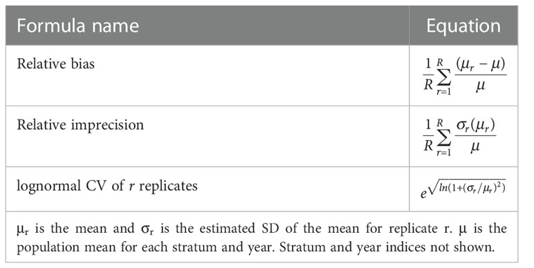
Table 1 Formulas used to compare relative bias and imprecision of glider sampling for R replicates at each maximum dive depth.

Acoustic backscatter values obtained using gliders diving to the seven maximum depths were compared to those in the sample populations using four metrics: mean absolute error (MAE), root mean squared error (RMSE), relative bias, and relative imprecision (Mier and Picquelle, 2008; Chai and Draxler, 2014) (Table 2). The units of all these metrics are the units of the samples, s_A in this case. These four metrics were calculated for all years combined within each stratum, for each maximum dive depth, and for 1 to 5 gliders. The MAE penalizes all errors equally while the RMSE penalizes poorer fits more than closer fits because the errors are squared. Thus RMSE ≥ MAE.

TABLE 2

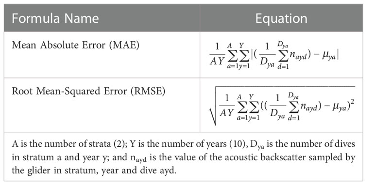
Table 2 Formulas used to compare the fits of a single replicate glider sample in stratum a, year y and dive d to the population means (μ_ya).

Knowing the population values being estimated permitted the accuracy of these estimates to be assessed by calculating the coverage probability: the proportion of depth-integrated population densities that were within one SD of the sample means. The coverage probability could then be compared to its expected value of 0.68. When > 68% of the population values are within one SD of the sample means, accuracy is better (a “conservative” estimate of the sample SD) than estimated from the samples. When< 68% of the population densities are within one SD of the sample mean the sampling is less accurate (a “permissive” estimate) than estimated.

2.6. The delta distribution

Various alternative methods to those used here have been suggested to reduce the variance of individual samples from skewed distributions. Many of these alternatives were developed to address issues with using samples in non-linear regressions to standardize fisheries catch and effort data or to predict species abundance based on environmental or other ecological covariates (e.g. Barry and Welsh, 2002). The delta approach (Pennington, 1983; Pennington, 1996; Lo et al., 1992; Steffanson, 1996; Maunder and Punt, 2004) is a family of methods that model the probabilities of the zero catches and of the values greater than zero with two separate probability distributions. Jolly and Hampton (1990a); Jolly and Hampton (1990b) pointed out that distributional assumptions such as those made in the delta approach are not required for unbiased estimates of population mean and variance in design-based surveys. Syrjala (2000) noted that the delta approach can be sensitive to small departures from the assumed error distributions and was a positively biased estimator of the mean for the demersal trawl data in that study.

As a potential alternative to the lognormal CV calculation used for calculating SDs in this study (Table 1), we applied the delta approach to the glider samples using the “deltadist” function from the R package “fishmethods (v. 1.11-0)” (Nelson, 2018) using dive-specific, integrated backscatter samples as the sampling unit. The deltadist approach models dives with zero acoustic density as binomially distributed and those with positive density as lognormal.

3. Results

3.1. Sample population

The population values created from the ship data were highly variable and zero-inflated. These characteristics differed with depth. Acoustic energies (s_A) were highest at depths of about 50 to 60 m, decreasing towards zero at shallower or deeper depths (Figure 3). The coefficients of variation (CV) for the combined database of both strata and all years ranged from about 20 times the mean values at 5 to 50 m depth to 50 to 100 times the means at deeper depths (Figure 4A). The proportion of cells at depth with zero energy (Figure 4B) was inversely related to total energy (Figure 3), increasing from over 50% at 40 to 50 m depth to over 90% at shallower and deeper depths (Figure 4B). 92% of the mean annual acoustic energy was in 0.1% of the grid cells in each strata. The annual mean proportion of cells with greater than 0 acoustic energy was 19% for Bransfield Strait and 23% for Cape Shirreff. Bransfield Strait in 2004 had the smallest proportion, 3%, of sample bins with 0 acoustic energy of all years in either stratum. Additional population variability occurred among strata and years (Supplementary Table S1).

FIGURE 3

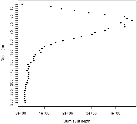
Figure 3 Mean nautical area scattering coefficients (s_A) in fifty 5 m depth bins of the 20 populations being sampled by simulated gliders for both strata and all years combined.

FIGURE 4

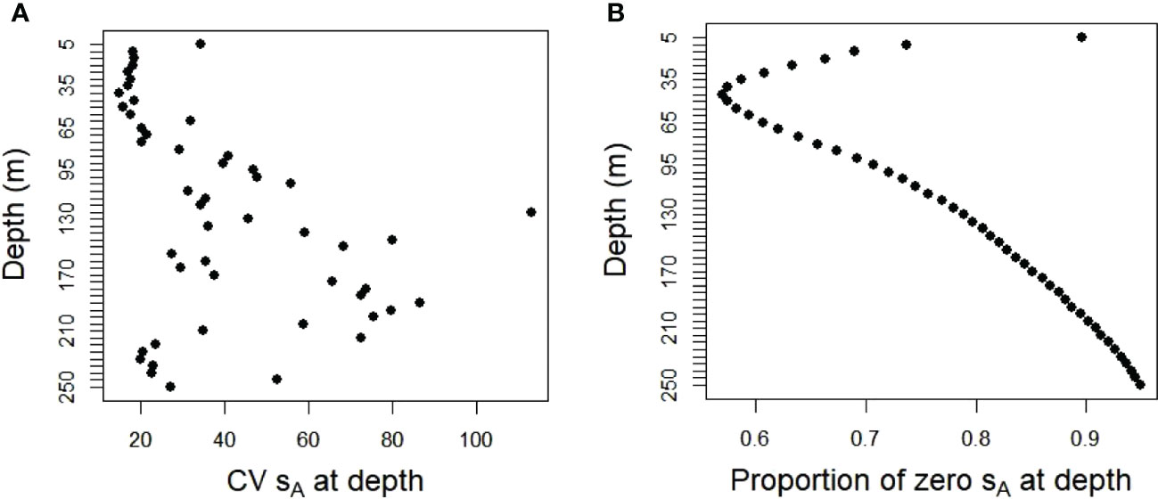
Figure 4 (A) CVs of acoustic energy and (B) proportions with zero energy in fifty 5 m depth bins in the 20 populations sampled by the simulated gliders for both strata and all years combined.

3.2. Single gliders

The number of 150 m dives completed annually in a strata depended on the amount of trackline miles available in the ship-derived data and ranged from 134 to 564 (Supplementary Table S3). The means and SDs from 500 replicates of a single glider fitted the depth-integrated population densities well, with wider variability among gliders diving to 1000 m compared to those diving to 150 m (Figure 5). Annual population mean s_A values for the two strata ranged from about 55 to 2981 (logged values of 4 to 8). The population values were within a SD of the 500 replicate sample estimates.

FIGURE 5

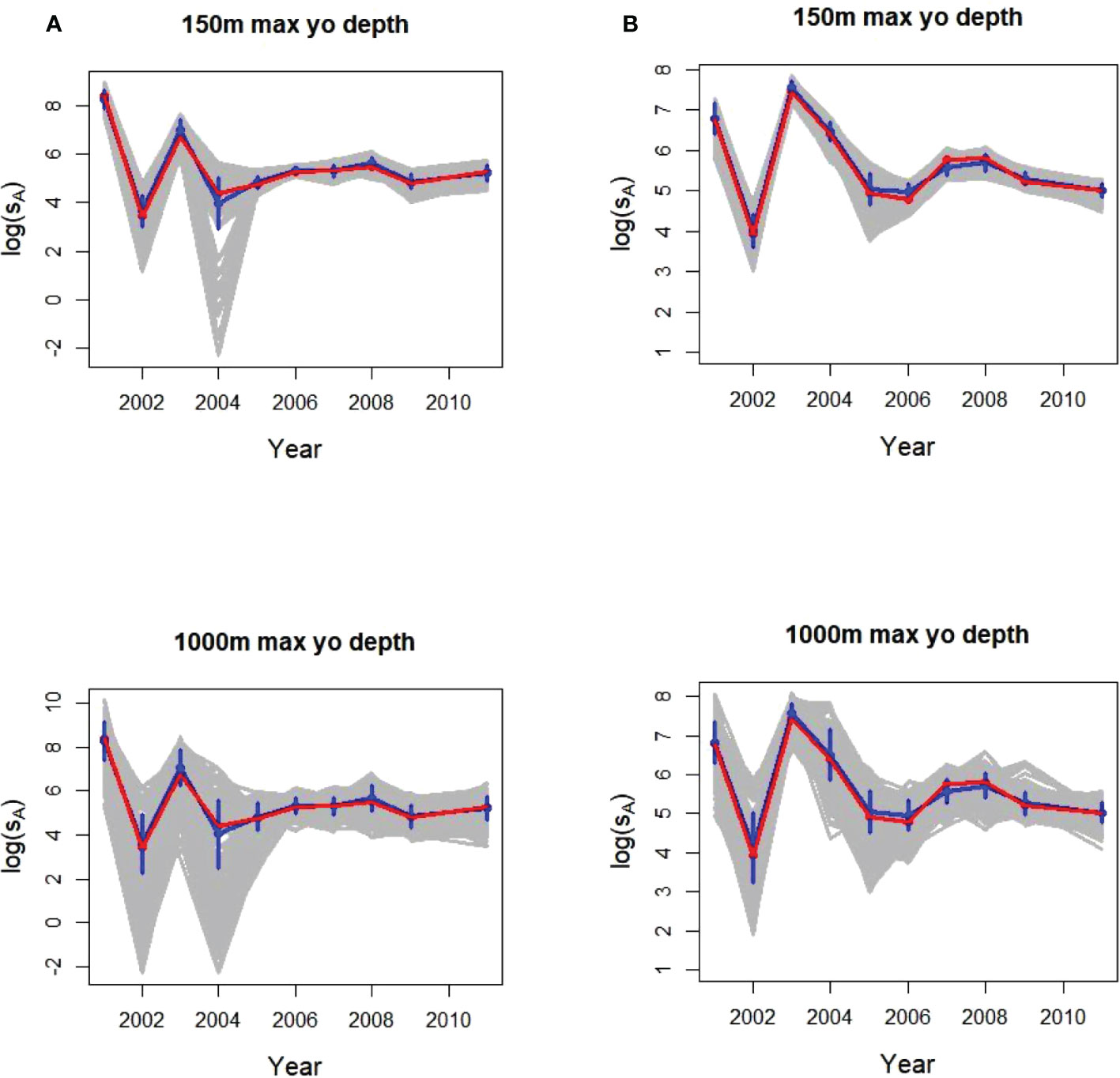
Figure 5 Annual glider logged sample means and SDs (blue) from 500 individual replicates (gray) of 1 glider with a maximum dive depths of 150 m (top plots) and 1000 m (bottom) sampling acoustic energy (s_A) in (A) Bransfield Strait and (B) Cape Shirreff. In all plots, the population means being sampled (from the original ship surveys) are in red.

The vertical distribution of krill acoustic densities at depth within the upper 250 m of the water column before depth-integrated energies were calculated was captured in the samples from a single glider replicate (Figure 6). The highest acoustic energies were found at depths of less than 150 m in Bransfield Strait and less than 125 m in Cape Shirreff for most years in both the glider samples and the populations. The concentrations of high energies in 2001 and 2003 in Bransfield Strait and in 2003 and 2007 in Cape Shirreff were apparent in the samples for each strata from a single glider selected at random (Figure 6, bottom).

FIGURE 6

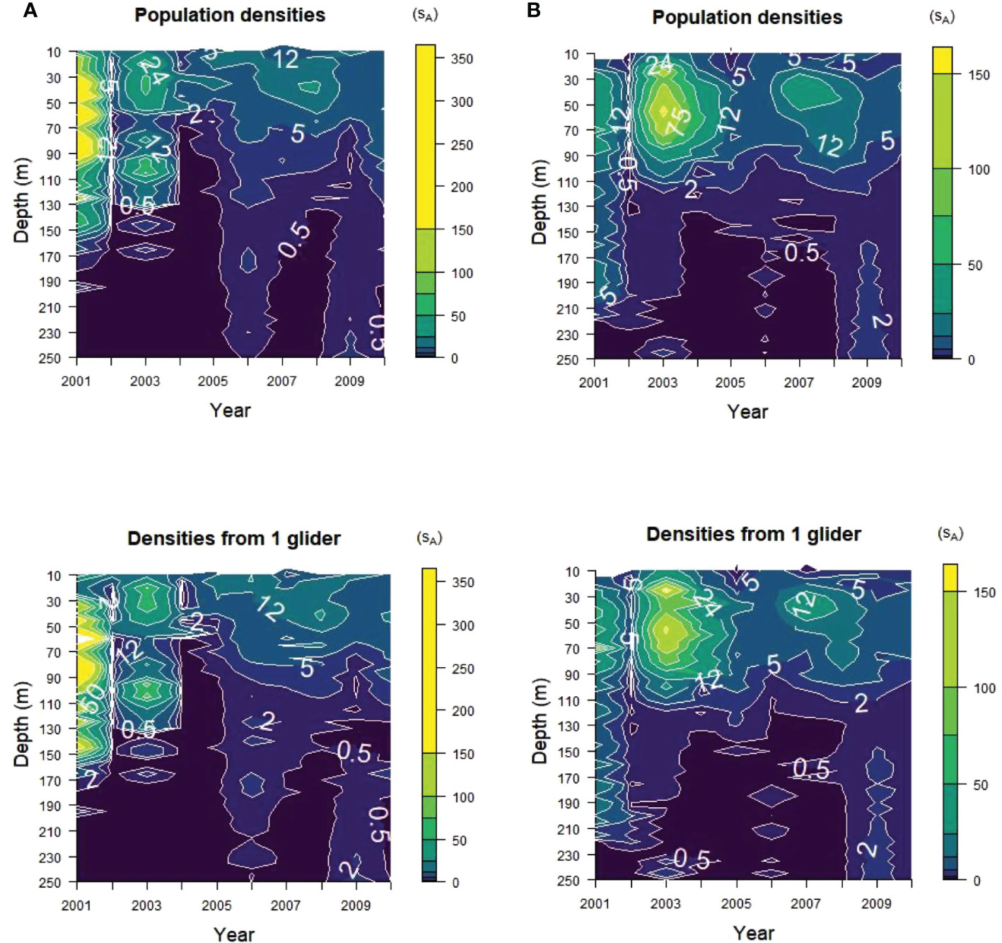
Figure 6 Acoustic energy contours with depth from (A) Bransfield Strait and (B) Cape Shirreff. The true energies (“Population densities”) and one randomly selected glider replicate with maximum dives of 150 m (“Densities from 1 glider”) are shown. Note the scale differences between the two strata, with higher maximum densities for Bransfield Strait than for Cape Shirreff.

3.3. Increasing maximum dive depth and glider fleet size

The best fits to the depth-integrated krill acoustic energies as represented by the MAE and RMSE scores in both strata were obtained with a maximum dive depth of 150 m, improving as the numbers of gliders at that maximum depth increased from 1 to 5 (Figure 7). The generally lower (better) scores from Cape Shirreff for the equivalent number of gliders and maximum dive depth indicated the Cape Shirreff gliders estimated the true s_A better than those sampling Bransfield Strait, likely because either because Cape Shirreff had nearly twice the trackline length available for glider sampling or because Cape Shirreff had a less zero-inflated distribution (Supplementary Table S1), or both. In all cases the worst fits were for fewer gliders diving at deeper depths. The RMSE scores were over twice as high for 1 glider sampling at maximum depth of 1000 m compared to 1 glider sampling at 150 m (Figure 7), indicating the 150 m glider fitted the population values over twice as well as the 1000 m glider. As the number of gliders sampling at 150 m increased from 1 to 5 the RMSE improved from about 250 s_A to 150 s_A for Bransfield Strait and from about 110 to less than 80 s_A for Cape Shirreff.

FIGURE 7

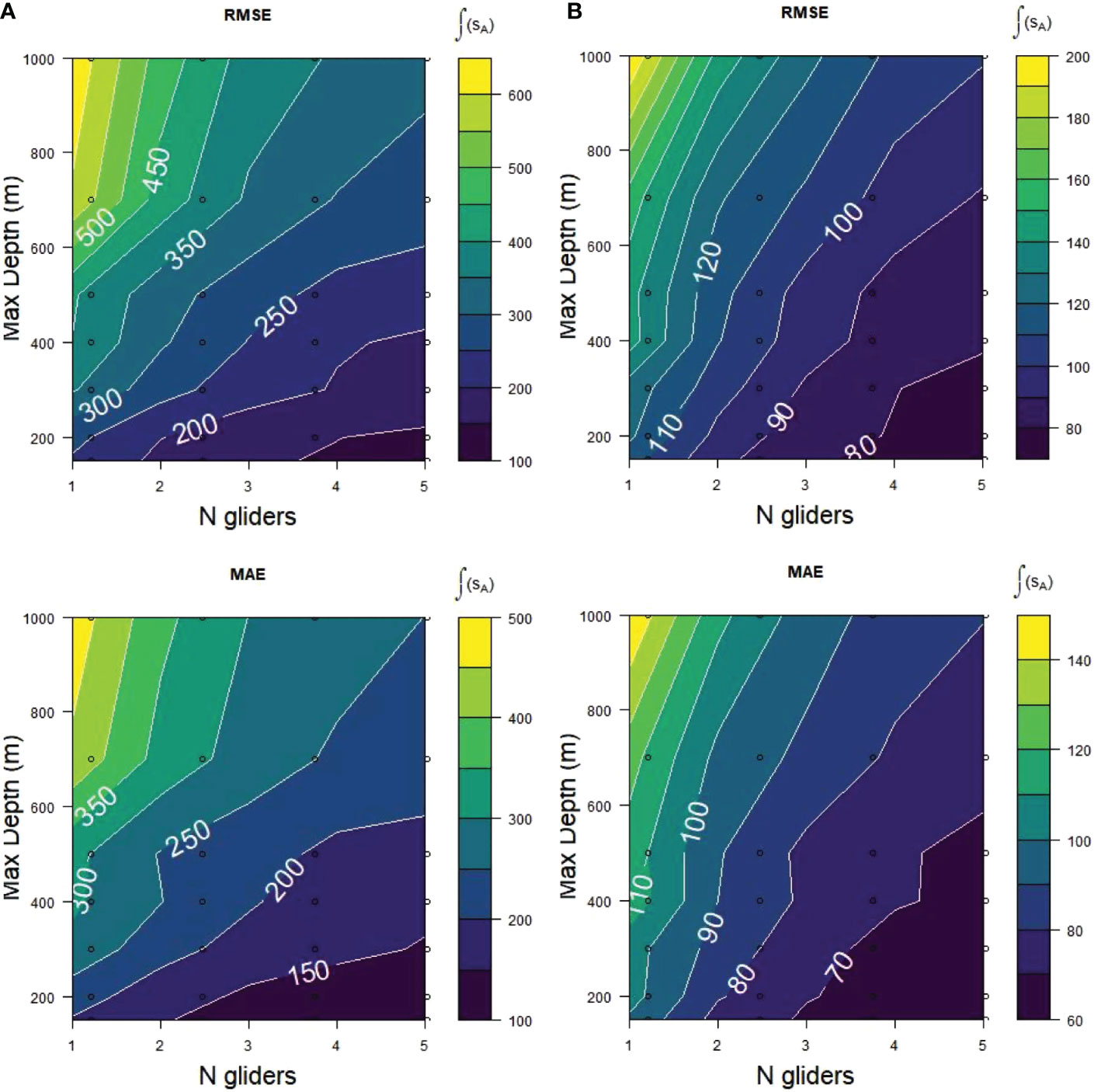
Figure 7 RMSE and MAE scores for acoustic samples (s_A) from (A) Bransfield Strait and (B) Cape Shirreff obtained at 7 maximum dive depths from 150 to 1000 m with 1 to 5 simulated gliders during 2001 to 2011. Each plot represents mean scores of 500 replicates during 10 years. Lower scores (darker colors) represent better fits of the glider sampling to the sample populations.

The patterns of MAE were similar to those of the RMSE (Figure 7), although with smaller absolute values. As already mentioned, this is the result of MAE measuring absolute and RMSE measuring squared differences between the sample and population values.

Decomposing RMSE into its basic components, bias and precision (Table 2; Figure 8), demonstrated that bias in the glider samples was small and apparently random. Bias did not vary systematically with maximum dive depth. There was a possible indication of smaller bias for 1 than for multiple gliders but the small values and lack of a consistent pattern were inconclusive. Imprecision of the glider samples was sensitive to both the number of gliders and maximum dive depth. It was lower (better) at 150 m maximum dive depth as the number of gliders increased from 1 to 5. Imprecision worsened with increases in maximum dive depth.

FIGURE 8

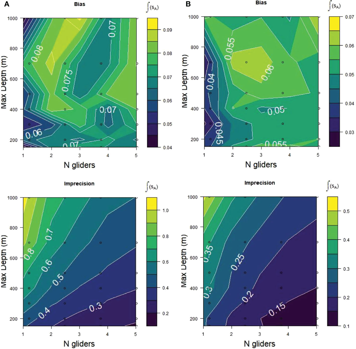
Figure 8 Relative bias and relative imprecision for acoustic samples (s_A) from (A) Bransfield Strait and (B) Cape Shirreff obtained from the same sampling alternatives as for Figure 7. Lower scores/darker colors are better fits of the glider samples to the populations being sampled.

Coverage probabilities for 1, 3 and 5 gliders diving to 150 m maximum depth in each stratum and year were near 1 from 2005 to 2011 (Figure 9). This indicates the SDs calculated from glider samples included the population mean nearly 100% of the time, better coverage than the 68% nominal value from sampling theory. In only one strata and year, Bransfield Strait in 2004, was the coverage for one glider diving to 150 m less than 68%. Coverages for all years in both strata were greater than 68% when 3 or 5 gliders were used.

FIGURE 9

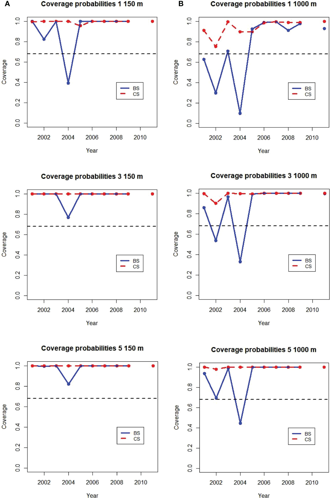
Figure 9 Annual coverage probabilities of 1, 3, and 5 gliders sampling at (A) 150 m (0.9 km trackline/dive) and (B) 1000 m (4.5 km/dive) maximum dive depth in the Bransfeld Strait (BS) and Cape Shirref (CS) strata. The expected value of 68% is shown as the dashed black line. No ship samples were available from 2010.

For gliders diving to 1000 m coverage probabilities were less accurate. For one 1000 m glider coverage probability was better than 68% for all years at Cape Shirreff but less than 68% for three of the 10 years in Bransfield Strait. Two years in Bransfield strait had coverages less than 68% with three gliders diving to 1000 m and Bransfield Strait in 2004 continued to have coverage less than 68% with 5 gliders. The poorest coverages were for the years with the highests proportions of cells with zero acoustic energy (Supplementary Table S1).

3.4. The delta distribution

In contrast to the method using the lognormal CV (Table 2) to calculate the SDs and coverage probabilities (Figures 5, 9) the deltadist method applied to the simulated glider data for 150 m maximum depths produced mean and SDs of acoustic energy in many years that did not include the population value despite the delta distribution SDs being larger than those calculated from the lognormal CV (compare Figure 5 with Figure 10). This was particularly evident for the Cape Shirreff samples in 2004 and 2007, for which the population values were outside the 95% CIs (twice the SD bars shown) (Figure 10).

FIGURE 10

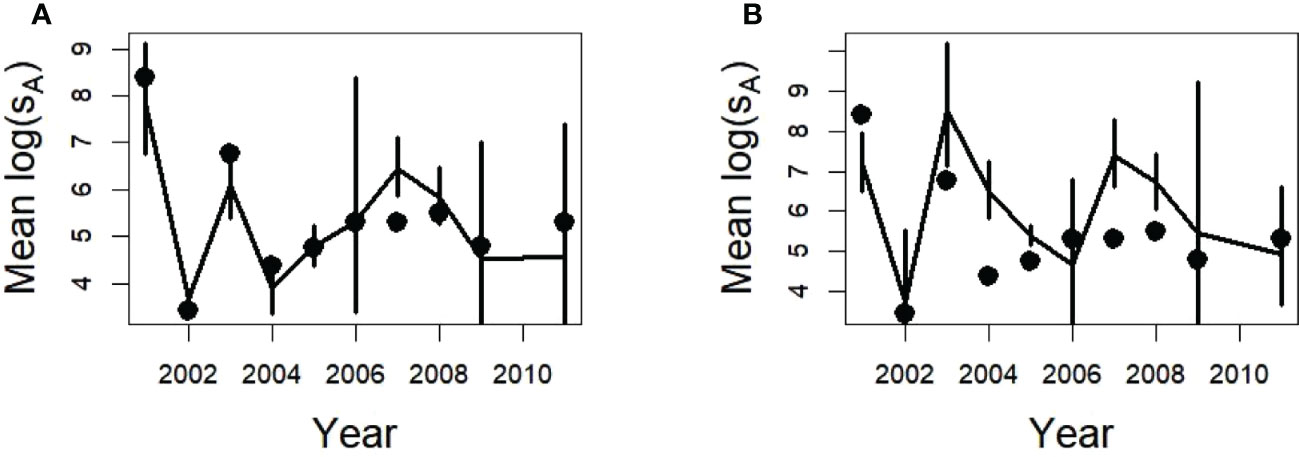
Figure 10 Estimated densities using the delta distribution and dives as the sampling unit ± one SD from 500 replicates of a single glider (lines) with a maximum depth of 150 m for Bransfield Strait (A) and Cape Shirreff (B), and the annual mean densities of the population (points).

4. Discussion

Simulated acoustically-equipped buoyancy gliders sampling krill backscatter originally collected by ships in two sample strata during 10-years produced estimates of depth-integrated acoustic backscatter with SDs that included the population means for the majority of the glider samples. The angled swath of acoustic data collected by gliders was able to represent the mean integrated acoustic energy of both strata on an annual basis. This sawtooth pattern of glider sampling should be adequate for estimating acoustic energies of any acoustically detectable species if the glider is able to complete enough dives so that the zero-inflation and overdispersion commonly encountered for marine organisms are mediated.

The number of dives to be completed for a given confidence level will probably depend on the scale of patchiness for the target species. In practice, gliders may collect oceanographic and other data in addition to acoustic measurements, so modeling the effect of making deeper dives on estimates of krill acoustic energies within the upper 250 m of the water column while still collecting oceanographic data below 150 m was a motivation for this study. Despite high proportions of individual dives sampling zero energy for some years it wasn’t until the proportion of zeros in the sample population reached 95% that the coverage probabilities of the sampling fell below 68%. These results suggest glider surveys with over 90% of dives measuring zero energy values may still be adequate at representing the mean population values, but as these zero proportions reach 95% additional glider dives might be required.

Subsampling large acoustic datasets has been found to be an effective method of estimating parameters in other studies (e.g., Levine and De Roberts, 2019). However, sampling from finite datasets may constrain what can be achieved. As previously noted, data limitations reduced the number of samples available to simulate gliders diving to deeper dive depths. The range of from 20 to 87 sampling dives at 1000 m permited by these population datasets performed less well than the 218 to 543 dives possible at 150 m (Supplementary Table S3).

Some studies of patchily distributed species identify individual swarms or schools of the target species from glider acoustic data to estimate population parameters (e.g. Coetzee, 2000; Guihen et al., 2014). This target identification step was already conducted using dB-differencing in the database being sampled by the simulated gliders. The approach used here does not require identification of swarms or schools to estimate density.

All acoustic sampling of pelagic populations requires a time interval to be completed. The trackline distances sampled in this study were completed in 4 or 5 days by the ship surveys but would require a month or more to be completed by an individual glider. The evaluation of glider sampling properties did not explicitly address temporal differences between sampling with gliders and with ships. The assumption here was that the distribution sampled by a ship in 4 or 5 days is a plausible model for the distribution encountered by a glider over months of sampling (though multiple gliders would reduce the time needed to survey a given area). Because the gliders move slowly (~ 0.5 knots) relative to a ship (~ 10 knots), it is important to consider the potential effects of temporal variation in the density of the target species. Within a given survey area, data collected by slow moving gliders will likely include more temporal variation in the density of the target species than would be the case if the area was surveyed by a fast moving ship. Also, there is the potential for slower-moving gliders to sample the same target more than once (i.e. Guihen, 2018). In the first two seasons of U.S. AMLR field sampling with gliders in the Bransfield Strait and Cape Shirreff strata, individual gliders averaged about 19 km/day (CSR, personal observation). Sampling at this speed, a single glider would take about 20 days to complete 380 km at a maximum dive depth of 150 m. Simultaneous sampling with 5 gliders day and night over 20 days could potentially sample 1900 km, more than completed by ships during the 4 or 5 day period they sampled in Bransfield Strait (10-year range 376 to 1008 km) or Cape Shirreff (1162 to 1582 km).

If there are actually temporal differences in krill distribution that were not captured by the ship samples over the several days during which they were obtained, such as seasonal differences in the highest concentrations of density with depth, the optimal sampling scheme identified here (dive profile to 150 m depth) might need to be modified. Glider-based sampling over a longer period of time could be advantageous, relative to ships, in estimating an annual density index of the target species and its variability because temporal variability undetected during short ship surveys could be sampled by gliders.

Multiple gliders sampling over longer time periods than a ship survey could improve understanding of seasonal variation in the population dynamics of the target species. Other researchers have pointed to the potential utility of coordinated communication with feedback among gliders during a survey (e.g. Leonard et al., 2010) or of using gliders as part of a larger survey system that includes other platforms such as ships and moorings (Handegard et al., 2013). In addition to gliders, the U. S. AMLR Program is currently deploying instrumented moorings at fixed locations to sample the temporal variability of krill densities over the course of a year. Acoustic surveys conducted by the fishery have also been initiated (e.g., Krafft et al., 2021). These moorings and surveys are in the same locations around the Antarctic Peninsula that the gliders will be sampling. Future field and modeling research will be able to compare the estimated densities using gliders to those obtained at the fixed moorings and by the fishery over time in the same region.

Some studies (e.g. Yu et al., 2012) have found adaptive cluster sampling, in which sampling intensity is modified based on observed densities during the survey, to be advantageous for species with patchy distributions. Mier and Picquelle (2008) compared six sampling designs and found that both a stratified systematic design with accurate prior information on densities, followed by an unstratified systematic survey with a random starting point when prior information was unavailable, performed better than adaptive sampling designs for larval walleye pollock (Gadus chalcogrammus). Adaptive sampling may not be practical for gliders. At present, acoustic data from gliders are not routinely telemetered back to the home laboratory because of data-processing limitations on board the vehicle and bandwidth limitations during satellite communications. Even if such issues are resolved by improved technologies, the slow movement of gliders will introduce time lags between measuring high densities of the target species within an appropriately sized area and vectoring another platform to the area (or changing the mission of the glider that originally recorded the high densities). The practicality of adaptive sampling with gliders might be improved if fleets of gliders are able to communicate with one another (e.g. Leonard et al., 2010), and appropriate sampling schemes can be pre-programmed into the vehicles (e.g., Glider 1 switches to shallow dives if Glider 2 identifies the target species in the upper water column). In the meantime, we recommend using prior knowledge about oceanographic conditions or habitats to design surveys that are prosecuted by multiple gliders simultaneously sampling at multiple scales. For example, one glider could conduct a highly resolved survey of an area expected to contain a high density of the target species while a second glider conducted a less resolved survey of the surrounding area.

The apparent ability of gliders to reproduce the distribution of target species density with depth (Figure 6) suggests another possibility for future research. Some studies have indicated that an appreciable portion of krill, as high as 20% of the total, could be located below the depths detectable using ship acoustics (Clarke and Tyler, 2008; Brierley, 2008; Schmidt et al., 2011). Deep diving gliders could provide information about krill located below typical survey depths, although krill directly on the sea floor would still be difficult to detect acoustically. This should be the case for other target species as well.

At relatively high frequencies (e.g., 200 kHz), the quality of ship-based acoustic data tend to degrade at ranges deeper than about 250 m using standard operational methods, e.g. maximum recommended input power (Korneliussen et al., 2008). In contrast, a glider can sample to 1000 m during dives to 900+ m with consistent signal quality at 200 kHz up to 100 m below the vehicle. A trade-off in the glider case is that the entire 1000 m cannot be sampled at a single instant using the echosounders currently available for gliders. Instead, the many 100 m range samples must be considered to represent the 1000 m water column over the period of time it takes the glider to descend from the surface to 900 m.

A critical aspect of any acoustic survey is target identification; this poses challenges for glider surveys of fisheries resources (e.g., Fallon et al., 2016). In the Southern Ocean, krill were historically collected by net tows for target identification and converting acoustic returns to biomass (Reiss et al., 2008). However, krill length distributions can also be obtained from the commercial fishery and from predator diets, and these distributions can track those from nets (Reid et al., 1999; Brierley et al., 2002; Miller and Trivelpiece, 2007). The U.S. AMLR Program is exploring the use of diet samples from krill predators (seabirds and pinnipeds), rather than nets towed by research vessels, to collect length-frequency data on krill. Such alternatives might not be available for other target species.

We are also developing methods to facilitate target identification by attaching cameras to gliders (e.g., Fernandes et al., 2016) and using artificial intelligence algorithms (e.g., the Video and Image Analytics for Multiple Environments, VIAME, available on GitHub) to identify targets from the photos collected during a glider’s flight. Such instruments and techniques have potential for estimating the lengths of krill, in addition to those mentioned above. Glider-borne cameras might also help identify targets located on the sea floor.

4.1. Conclusion

Calibrating the new glider-based acoustic data with historic ship-based data on krill densities will be critical to using glider sampling to understand the ecology and population dynamics of this species, its fishery, and other Antarctic species that depend on krill as prey. These simulations support the proposition that the sawtooth pattern of sampling by gliders can provide a time series of survey estimates that is statistically compatible with the historical series collected by ships. Additional field studies to evaluate similarities and differences produced by various platforms such as gliders, ships, and moorings acoustically sampling the population dynamics of krill in the same regions of the Antarctic peninsula are being conducted. Combining the data from these and similar platforms into an integrated assessment of the status and trends in krill population dynamics could potentially be assembled in the future. The methods applied here could be applicable to evaluating other potential glider surveys of patchily-distributed organisms.

Data availability statement

The datasets and R scripts (R Core Team (2022)) used in this study can be found in online repositories. The names of the repository/repositories and accession number(s) can be found below: https://github.com/us-amlr/glider-simulation.

Author contributions

All authors listed have made a substantial, direct and intellectual contribution to the work, and approved it for publication.

Acknowledgments

This research was conducted under NOAA base funding. George Cutter and Jen Walsh provided a number of suggestions and constructive comments that improved the approach and narrative. We thank our reviewers, Patrick Lehodey and Christophe Guinet, for their recommendations and advice.

Conflict of interest

The authors declare that the research was conducted in the absence of any commercial or financial relationships that could be construed as a potential conflict of interest.

Publisher’s note

All claims expressed in this article are solely those of the authors and do not necessarily represent those of their affiliated organizations, or those of the publisher, the editors and the reviewers. Any product that may be evaluated in this article, or claim that may be made by its manufacturer, is not guaranteed or endorsed by the publisher.

Supplementary material

The Supplementary Material for this article can be found online at: https://www.frontiersin.org/articles/10.3389/fmars.2022.1064181/full#supplementary-material

References

Alonzo S. H., Switzer P. V., Mangel M. (2003). An ecosystem-based approach to management: using individual behavior to predict the indirect effects of Antarctic krill fisheries on penguin foraging. J. Appl. Ecol. 40, 692–702. doi: 10.1046/j.1365-2664.2003.00830.x

CrossRef Full Text | Google Scholar

Barry S. C., Welsh A. H. (2002). Generalized additive modeling and zero inflated count data. Ecol. Model. 157, 179–188. doi: 10.1016/S0304-3800(02)00194-1

CrossRef Full Text | Google Scholar

Benoit-Bird K. J., Welch T. P., Waluk C. M., Barth J. A., Wangen I., McGill P., et al. (2018). Equipping an underwater glider with a new echosounder to explore ocean ecosystems. Limnol. Oceanogr.: Methods 16, 734–749. doi: 10.1002/lom3.10278

CrossRef Full Text | Google Scholar

Brierley A. S. (2008). Antarctic Ecosystem: are deep krill ecological outliers or portents of a paradigm shift? Curr. Biol. 18 (6), 252–254. doi: 10.1016/j.cub.2008.01.022

CrossRef Full Text | Google Scholar

Brierley A. S., Goss C., Grant S. A., Watkins J. L., Reid K., Belchier M., et al. (2002). Significant intra-annual variability in krill distribution and abundance at south Georgia revealed by multiple acoustic surveys during 2000/01. CCAMLR Sci. 9, 71–82.

Google Scholar

CCAMLR (2018). Available at: https://www.ccamlr.org/en/document/publications/krill-fishery-report-2018.

Google Scholar

CCAMLR Fishery Report. (2021). Euphausia superba in Area 48. CCAMLR Secretariat. Available at: https://fishdocs.ccamlr.org/FishRep_48_KRI_2021.pdf.

Google Scholar

Chai T., Draxler R. R. (2014). Root mean square error (RMSE) or mean absolute error (MAE)? –arguments against avoiding RMSE in the literature. Geosci. Model. Dev. 7, 1247–1250. doi: 10.5194/gmd-7-1247-2014

CrossRef Full Text | Google Scholar

Chave R., Buermans J., Lemon D. D., Taylor J. C., Lembke C., DeCollibus C., et al. (2018). “Adapting multi-frequency echo-sounders for operation on autonomous vehicles,” Proceedings of the OCEANS 2018 MTS/IEEE Charleston Charleston, SC. doi: 10.1109/OCEANS.2018.8604815

CrossRef Full Text | Google Scholar

Clarke A., Tyler P. A. (2008). Adult Antarctic krill feeding at abyssal depths. Curr. Biol. 18, 282–285. doi: 10.1016/j.cub.2008.01.059

PubMed Abstract | CrossRef Full Text | Google Scholar

Coetzee J. (2000). Use of a shoal analysis and patch estimation system (SHAPES) to characterise sardine schools. Aquat. Living Resour. 13, 1–10. doi: 10.1016/S0990-7440(00)00139-X

CrossRef Full Text | Google Scholar

Croxall J. P., Nicol S. (2004). Management of bransfield strait ocean fisheries: global forces and future sustainability. Antarctic Sci. 16 (4), 569–584. doi: 10.1017/S0954102004002330

CrossRef Full Text | Google Scholar

Croxall J. P., Prince P. A., Reid K. (1997). Dietary segregation of krill-eating south Georgia seabirds. J. Zool. 242, 531–556. doi: 10.1111/j.1469-7998.1997.tb03854.x

CrossRef Full Text | Google Scholar

De Robertis A., Lawence-Slavas N., Jenkins R., Wangen I., Mordy C. W., Meinig C., et al. (2019). Long-term measurements of fish backscatter from saildrone unmanned surface vehicles and comparison with observations from a noise-reduced research vessel. ICES J. Mar. Sci. 76, 2459–2470. doi: 10.1093/icesjms/fsz124

CrossRef Full Text | Google Scholar

Dichmont C. M., Deng A., Punt A. E., Venables W., Haddon M. (2006). Management strategies for short-lived species: The case of australia’s northern prawn fishery 1. accounting for multiple species, spatial structure and implementation uncertainty when evaluating risk. Fish. Res. 82, 204–220. doi: 10.1016/j.fishres.2006.06.010

CrossRef Full Text | Google Scholar

Fallon N. G., Fielding S., Fernandes P. G. (2016). Classification of southern ocean krill and icefish echoes using random forests. ICES J. Mar. Sci. 73 (8), 1998–2008. doi: 10.1093/icesjms/fsw057

CrossRef Full Text | Google Scholar

Fernandes P. G., Brierley A. S., Simmonds E. J., Millard N. W., McPhail S. D., Armstrong F., et al. (2000). Fish do not avoid survey vessels. Nature 404, 35–36. doi: 10.1038/35003648

PubMed Abstract | CrossRef Full Text | Google Scholar

Fernandes P. G., Copland P., Garcia R., Nicosevici T., Scoulding B. (2016). Additional evidence for fisheries acooustics: small cameras and angling gear provide tilt angle distributions and other relevant data for mackeral surveys. ICES J. Mar. Sci. 73 (8), 2009–2019. doi: 10.1093/icesjms/fsw091

CrossRef Full Text | Google Scholar

Fernandes P. G., Gerlotto F., Holliday D. V., Nakken O., Simmonds E. J. (2002). Acoustic applications in fisheries science: the ICES contribution. ICES Mar. Sci. Symp. 215, 483–492. doi: 10.17895/ices.pub.8889

CrossRef Full Text | Google Scholar

Fielding S., Watkins J. L., Collins M. A., Enderlein P., Venables H. J. (2012). Acoustic determination of the distribution of fish and krill across the Scotia Sea in spring 2006, summer 2008 and autumn 2009. Deep-Sea Res. II. 59-60, 173–188. doi: 10.1016/j.dsr2.2011.08.002

CrossRef Full Text | Google Scholar

Greene C. H., Meyer-Gutbrod E. L., McGarry L. P., Hufnagle L. C. Jr., Chu D., McClatchie S., et al. (2014). A wave glider approach to fisheries acoustics: Transforming how we monitor the nation’s commercial fisheries in the 21st century. Oceanography 27 (4), 169–174. Available at: https://www.jstor.org/stable/24862221#metadata_info_tab_contents

Google Scholar

Guihen D. (2018). High-resolution acoustic surveys with diving gliders come at a cost of aliasing moving targets. PloS One 13 (8), e0201816. doi: 10.1371/journal.pone.0201816

PubMed Abstract | CrossRef Full Text | Google Scholar

Guihen D., Brearley J. A., Fielding S. (2022). Antarctic Krill likely avoid underwater gliders. Deep-Sea Res. I 179, 103680. doi: 10.1016/j.dsr.2021.103680

CrossRef Full Text | Google Scholar

Guihen D., Fielding S., Murphy E. J., Heywood K. J., Griffiths G. (2014). An assessment of the use of ocean gliders to undertake acoustic measurements of zooplankton: the distribution and density of Antarctic krill (Euphausia superba) in the weddell Sea. Limnol. Oceanogr.: Methods 12, 373–389. doi: 10.4319/lom.2014.12.373

CrossRef Full Text | Google Scholar

Handegard N. O., du Buisson L., Brehner P., Chalmers S. J., De Robertis A., Huse G., et al. (2013). Towards an acoustic-based coupled observation and modelling system for monitoring and predicting ecosystem dynamics of the open ocean. Fish. Fish. 14, 605–615. doi: 10.1111/j.1467-2979

CrossRef Full Text | Google Scholar

Hinke J., Cossio A. M., Goebe M. E., Reiss C. S., Trivelpiece W. Z., Watters G. M. (2017). Identifying risk: Concurrent overlap of the Antarctic krill fishery with krill-dependent predators in the Scotia Sea. PloS One 12 (1), e0170132. doi: 10.1371/journal.pone.0170132

PubMed Abstract | CrossRef Full Text | Google Scholar

Jolly G. M., Hampton I. (1990a). Some problems in the statistical design and analysis of acoustic surveys to assess fish biomass. Rapp. P -v Réun Cons. Int. Explor. Mer. 189, 415–420.

Google Scholar

Jolly G. M., Hampton I. (1990b). A stratified random design for acoutic surveys of fish stocks. Can. J. Fish. Aquat. Sci. 47, 1282–1291. doi: 10.1139/f90-147

CrossRef Full Text | Google Scholar

Kinzey D., Watters G. M., Reiss C. S. (2018). Parameter estimation using randomized phases in an integrated assessment model for Antarctic krill. PloS One 13 (8), e0202545. doi: 10.1371/journal.pone.0202545

PubMed Abstract | CrossRef Full Text | Google Scholar

Kinzey D., Watters G. M., Reiss C. S. (2019). Estimating recruitment variability and productivity in Antarctic krill. Fish. Res. 217, 98–107. doi: 10.1016/j.fishres.2018.09.027

CrossRef Full Text | Google Scholar

Korneliussen R. J., Diner N., Ona E., Berger L., Fernandes P. G. (2008). Proposals for the collection of multifrequency acoustic data. ICES J. Mar. Sci. 65, 982–994. doi: 10.1093/icesjms/fsn052

CrossRef Full Text | Google Scholar

Krafft B. A., Macaulay G. J., Skaret G., Knutsen T., Bergstad O. A., Lowther A., et al. (2021). Standing stock of Antarctic krill (Euphausia superba Dana 1850) in the southwest Atlantic sector of the southern ocean 2018-19. J. Crustacean Biol. 41 (3), 1–17. doi: 10.1093/jcbiol/ruab046

CrossRef Full Text | Google Scholar

Lembke C., Lowerre-Barbieri S., Mann D., Taylor J. C. (2018). Using three acoustic technologies on underwater gliders to survey fish. Mar. Technol. Soc. J. 52 (6), 39–52. doi: 10.4031/MTSJ.52.6.1

CrossRef Full Text | Google Scholar

Leonard N. E., Paley D. A., Davis R. E., Fratantoni D. M., Lekin F., Zhang F. (2010). Coordinated control of an underwater glider fleet in an adaptive ocean sampling field experiment in Monterey bay. J. Field Robotics 27 (6), 718–740. doi: 10.1002/rob.20366

CrossRef Full Text | Google Scholar

Levine M., De Roberts A. (2019). Don’t work too hard: Subsampling leads to efficient analysis of large acoustic datasets. Fish. Res. 219. doi: 10.1016/j.fishres.2019.105323

CrossRef Full Text | Google Scholar

Lo N. C. H., Jacobson L. D., Squire J. L. (1992). Indices of relative abundance from fish spotter data based on delta-lognormal models. Can. J. Fish. Aquat. Sci. 49, 2515–2526.

Google Scholar

MacLennan D. N., Fernandes P. G., Dalen J. (2002). A consistent approach to definitions and symbols in fisheries acoustics. ICES J. Mar. Sci. 59, 365–369. doi: 10.1006/jmsc.2001.1158

CrossRef Full Text | Google Scholar

Maunder M. N., Punt A. E. (2004). Standardizing catch and effort data: a review of recent approaches. Fish. Res. 70, 141–159. doi: 10.1016/j.fishres.2004.08.002

CrossRef Full Text | Google Scholar

Mier K. L., Picquelle S. J. (2008). Estimating abundance of spatially aggregated populations: comparing adaptive sampling with other survey designs. Can. J. Fish. Aquat. Sci. 65, 176–197. doi: 10.1139/f07-138

CrossRef Full Text | Google Scholar

Miller A. K., Trivelpiece M. W. (2007). Cycles of Euphausia superba recruitment evident in the diet of pygoscelid penguins and net trawls in the south Shetland islands, Antarctica. Polar Biol. 30, 1615–1623. doi: 10.1007/s00300-007-0326-7

CrossRef Full Text | Google Scholar

Nelson G. A. (2018). Fishmethods: Fishery science methods and models (R package version 1.11-0). Available at: https://cran.r-project.org/web/packages/fishmethods/index.html.

Google Scholar

Nicol S., Foster J., Kawaguchi S. (2012). The fishery for Antarctic krill – recent developments. Fish. Fish. 13, 30–40. doi: 10.1111/j.1467-2979.2011.00406.x

CrossRef Full Text | Google Scholar

Nicol S., Worby A., Leaper L. (2008). Changes in the Antarctic sea ice ecosystem: potential effects on krill and baleen whales. Mar. Freshw. Res. 59, 361–382. doi: 10.1071/MF07161

CrossRef Full Text | Google Scholar

Pennington M. (1996). Estimating the mean and variance from highly skewed marine data. Fish. Bull. 47, 1623–1624.

Google Scholar

R Core Team (2022). R: A language and environment for statistical computing (Vienna, Austria: R Foundation for Statistical Computing). Available at: https://www.R-project.org/.

Google Scholar

Reid K., Sims M., White R. W., Gillon K. W. (2004). Spatial distribution of predator/prey interactions in the Scotia Sea: implications for measuring predator/fisheries overlap. Deep-Sea Res. II 51, 1383–1396. doi: 10.1016/S0967-0645(04)00086-4

CrossRef Full Text | Google Scholar

Reid K., Watkins J. L., Croxall J. P., Murphy E. J. (1999). Krill population dynamics at south Georgia 1991–1997, based on data from predators and nets. Mar. Ecol. Prog. Ser. 177, 102–114. doi: 10.3354/meps177103

CrossRef Full Text | Google Scholar

Reiss C. S., Cossio A. M., Loeb V., Demer D. A. (2008). Variations in the biomass of Antarctic krill (Euphausia superba) around the south Shetland islands 1996-2006. ICES J. Mar. Sci. 65, 497–508. doi: 10.1093/icesjms/fsn033

CrossRef Full Text | Google Scholar

Reiss C. S., Cossio A. M., Santora J. A., Dietrich K. S., Murray A., Mitchell B. G., et al. (2017). Overwinter habitat selection by Antarctic krill under varying sea-ice conditions: implications for top predators and fishery management. Mar. Ecol. Prog. Ser. 568, 1–16. doi: 10.3354/meps12099

CrossRef Full Text | Google Scholar

Reiss C. S., Watters G., Cutter G., Cossio A. M., Walsh J. (2021). Glider-based estimates of meso-zooplankton biomass density: a fisheries case study on Antarctic krill (Euphausia superba) around the northern Antarctic peninsula. Front. Mar. Sci. doi: 10.3389/fmars.2021.604043

CrossRef Full Text | Google Scholar

Ruckdeschel G. S., Davies K. T. A., Ross T. (2020). Biophysical drivers of zooplankton variability on the scotian shelf observed using profiling electric gliders. Front. Mar. Sci. 7. doi: 10.3389/fmars.2020.00627

CrossRef Full Text | Google Scholar

Schmidt K., Atkinson A., Steigenberger S., Fielding S., Lindsay M. C. M., Pond D. W., et al. (2011). Seabed foraging by Antarctic krill: implications for stock assessment, benthopelagic coupling, and the vertical transfer of iron. Limnol. Oceanogr. 56, 1411–1428. doi: 10.4319/lo.2011.56.4.1411

CrossRef Full Text | Google Scholar

Steffanson G. (1996). Analysis of groundfish survey abundance data: combining the GLM and delta approaches. ICES J. Mar. Sci. 53, 577–588. doi: 10.1006/jmsc.1996.0079

CrossRef Full Text | Google Scholar

Syrjala S. E. (2000). Critique on the use of the delta distribution for the analysis of trawl survey data. ICES J. Mar. Sci. 57, 831–842. doi: 10.1006/jmsc.2000.0571

CrossRef Full Text | Google Scholar

Trenkel V. M., Handegard N. O., Weber T. C. (2016). Observing the ocean interior in support of integrated management. ICES J. Mar. Sci. 73 (8), 1947–1954. doi: 10.1093/icesjms/fsw132

CrossRef Full Text | Google Scholar

Yu H., Jiao Y., Su Z., Reid K. (2012). Performance comparison of traditional sampling designs and adaptive sampling designs for fishery-independent surveys: A simulation study. Fish. Res. 113, 173–181. doi: 10.1016/j.fishres.2011.10.009

CrossRef Full Text | Google Scholar

Pennington M. (1983). Efficient estimators of abundance, for fish and plankton surveys. Biometrics 39, 281–286. doi: 10.2307/2530830

CrossRef Full Text | Google Scholar