Benchmarking of automatic quality control checks for ocean temperature profiles and recommendations for optimal sets

1 Introduction

Ocean temperature profile observations are essential for many applications (Penny et al., 2019). These include those that require data in near real time such as ocean monitoring and forecasting (e.g. Chassignet et al., 2009; Blockley et al., 2014; King et al., 2018; Lellouche et al., 2018; Schiller et al., 2020) and numerical weather prediction from coupled atmosphere-ocean models (e.g. Dong et al., 2017; King et al., 2020). Ocean applications that require observations with less stringent timeliness requirements but a higher level of quality control include climate applications such as decadal forecasting (e.g. Dunstone and Smith, 2010; Bellucci et al., 2013), ocean/coupled atmosphere-ocean hindcast reanalyses (e.g. Balmaseda et al., 2015; Zuo et al., 2017; Laloyaux et al., 2018; Storto et al., 2019), ocean climate monitoring (e.g. Johnson et al., 2019; von Schuckmann et al., 2019; Gulev et al., 2021) and generation of climatologies (e.g. Gouretski and Koltermann, 2004; Schmidtko et al., 2013; Gouretski, 2019; Locarnini et al., 2019). In all cases, quality control (QC) of the data before use is required (Bushnell et al., 2019) to exclude from further consideration or use profiles and/or data points containing errors (e.g. sensor drifts, data stream errors, etc.), which may negatively impact results. QC may be performed using automatic methods or, ideally, through manual examination of the profiles by an expert human operator. In the case of near real time applications, the only viable way to perform the QC while still meeting timeliness requirements is by automatic checking. For delayed mode applications, the number of profiles in the historical archive makes expert manual examination of these profiles extremely challenging and time consuming. For example, there are more than 2.3 million eXpendable BathyThermograph (XBT) casts in the World Ocean Database (WOD; Boyer et al., 2018), with thousands of these being the largest source of temperature profile data for the 1980s and until the operational implementation of the Argo programme (Argo, 2021). Therefore, automatic QC (AQC) checking of historical data is essential for two purposes: (i) to allow the use of data within an acceptable time frame; and (ii) to identify profiles that are almost certain to contain only good quality data, reducing the number of profiles to be inspected by manual QC operators and making their task tractable. An overview of types of AQC checks considered in this study is presented below.

● Impossible date/time/depth - confirms that the date and time are possible (e.g. year is not unrealistically far in the past) and that depth is not negative;

● Ocean/sea location - checks that the profile location is not over land based on bathymetric data or a land/sea mask;

● Instrument track - compares the location of successive profiles from a sensor to detect unrealistic speeds or paths;

● Increasing depth/pressure - checks for instances whether depths/pressures do not increase through the profile;

● Constant values - detects repeated temperature values in the profile (e.g. due to sensor failure);

● Range - compares temperature values to a set of ranges, which may be defined globally or regionally and may change with depth;

● Gradient - checks for unrealistic temperature gradients through the profile;

● Spike/step - detects sudden changes in temperature in the profile, which may revert (spike) or continue further down the profile (step);

● Stability - detects temperature instabilities along the water column (i.e. density not increasing through the profile) within some tolerance range;

● Climatology/background - similar to a range check but the profile is compared to a climatological profile or a ‘background’ profile obtained through objective analysis, model forecast or other means, and thresholds may be defined using knowledge of the climatological/background and observation error variances;

● Fuzzy logic - instead of having a single test for a particular error mode which gives either a pass or reject result, fuzzy logic checks multiple features and uses the results together to assign a QC result in a fuzzy scale ranging from certainly pass to certainly reject;

● Machine learning - a broad category of data driven algorithms such as neural networks and Anomaly Detection which are able to classify the data quality based on non-linear criteria;

● XBT specific - XBTs have specific error modes such as sudden changes in the temperature profile when the wire that connects the instrument to the recorder breaks, and therefore specific QC tests have been set up for XBT data;

● Miscellaneous - QC checks that do not fit into the categories above such as comparison of profile depths to the maximum expected depth that an instrument might reach, or a check on the shape of the profile.

The gamut of AQC tests in use by the international community was largely developed by independent research groups and for their own varied applications and ocean regions (e.g. Gronell and Wijffels, 2008; UNESCO-IOC, 2010; Cabanes et al., 2013; Good et al., 2013; Garcia et al., 2018; Gouretski, 2018; Wong et al., 2020a; Gourrion et al., 2020b). There are a number of common types of QC procedure designed to detect frequently occurring error modes, and some for unique or uncommon errors. A non-exhaustive list of QC tests that fall into these categories is given in Table 1 and a detailed review can be found in Tan et al. (2022). Database managers and/or users will typically choose to apply a set of AQC checks to the profile data to detect a broad range of errors. To this date, however, there is no quantitative assessment of which AQC checks are the best performing.

TABLE 1

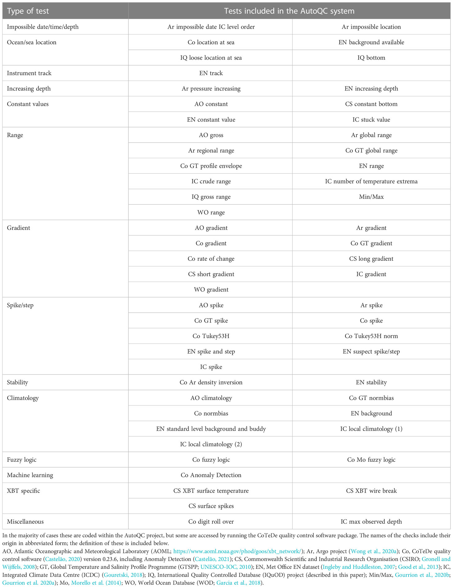
Table 1 List of types of QC checks and the individual tests that have been included in this study.

In this study, a comprehensive benchmarking exercise was carried out to evaluate the performance of sixty AQC checks (Table 1) and to recommend an optimal set of checks. This coordinated evaluation was performed as a strand of work of the International Quality Controlled Ocean Database (IQuOD) project (www.iquod.org) concerned with improving the QC applied to ocean temperature profiles using AQC (including machine learning). Other IQuOD work strands include cloud-based expert QC, development and assessment of algorithms for intelligently assigning metadata to profiles where they are missing (Palmer et al., 2018; Haddad et al., 2022), assignment of uncertainty estimates to each observation level of the profile (Cowley et al., 2021), flagging and removal of exact or near duplicates, and development of metrics to assess the impact of IQuOD activities. Overall, IQuOD’s aim is to improve the quality and consistency of historical ocean profile data and its value for scientific and societal services applications (Domingues and Palmer, 2015).

The benchmarking of the AQC checks in this study required two aspects for success: (i) a software infrastructure capable of processing a large set of profiles through a significant number of quality control checks; and (ii) reference data with known quality that can be used to benchmark the quality control checks and validate the results. Both (i) and (ii) are described in Section 2. Section 3 provides the benchmarking results and Section 4 their validation. Sections 5 and 6 respectively contain the discussion and conclusions.

2 Materials and methods

2.1 Software and methods

2.1.1 Software infrastructure

The software infrastructure used in this study was developed as a collaborative project using GitHub to host the code and track issues (https://github.com/IQuOD/). Repositories within the IQuOD GitHub project include wodpy (Mills et al., 2017), for file reader software for WOD data, and AutoQC, which contains the main code base for this project. The version of the AutoQC code used in this study can be found at https://github.com/IQuOD/AutoQC/releases/tag/publication-2022 (Good and Mills, 2022).

All code was developed in Python. The quality control checks listed in Table 1 were, in many cases, recoded from their original language into Python and/or restructured to allow them to all be run in a uniform way. We also made use of QC code that was written for the CoTeDe Python package (Castelão, 2020) by including ‘wrapper’ QC checks in AutoQC. These ‘wrapper’ checks run the CoTeDe software to obtain their QC decisions, allowing them to be used within the AutoQC software. QC checks have tests associated with them that run part or all of the QC algorithms to ensure that they are giving the expected answer and hence are working as intended.

The AutoQC processing chain has three main stages. The first is to create an SQLite database (www.sqlite.org). This holds the raw input data and has space for QC decisions from each quality control check contained in the software library and a set of reference QC flags. The second stage runs all the quality control checks on each profile and stores the results in the database. Finally, the third part of the processing is to run routines to obtain benchmark statistics and find optimal sets of quality control checks (‘IQuOD sets’).

The library of QC checks is designed to be easily expandable and reusable. All the QC checks produce results for the entire profile, and it is possible to run them in any order. If a new quality control check becomes available, it is only necessary to include it within the software library and the processing system will detect it and use it. It is expected that the processing will be repeated in the future when new reference data become available (see Section 5).

All software is available under the MIT license (https://github.com/IQuOD/AutoQC/blob/master/LICENSE) and hence is free for use by others within their systems. For example, Tan et al. (2022) successfully used the code to compare four different sets of QC tests. In the future, it is envisaged that the AutoQC code could be used in systems that provide AQC of profiles as they are collected.

2.1.2 New or modified QC checks

In most cases the QC checks included in the AutoQC repository are intended to be exact replicas of the original code. In a few cases, minor modifications or new tests were introduced to optimize functionality, as explained below.

2.1.2.1 Argo (Ar) impossible date

The Ar impossible date test was originally defined to check that the date of the profile is after 1 January 1997 (Wong et al., 2020a). While this is appropriate for Argo data, there are profiles from other instrument types that occur much earlier in the historical record. The date threshold was therefore set to 1700.

2.1.2.2 CSIRO (CS) XBT wire break

The CS XBT wire break test attempts to detect breaks in the wire that connects XBT probes to the surface by examining the change in temperature between adjacent levels in the profiles (Gronell and Wijffels, 2008). XBT wire breaks are a common error mode so it is important that these are detected. The CS XBT wire break test is the only quality control algorithm in the AutoQC system that is specifically designed for detecting this type of error. As described in Section 3.1, if the whole profile is rejected, the quality control flags from this test are reset to pass all levels.

2.1.2.3 Met Office (EN) background and standard level background and buddy

The EN processing system QCs profile data and then generates monthly objective analyses from them. The previous month’s analysis is used to create a ‘background’ which is used in the EN background QC checks (Ingleby and Huddleston, 2007; Good et al., 2013). In the absence of observations, the objective analyses relax to climatology. It was not possible to replicate the creation of monthly objective analyses in this study so instead these checks always use the climatology from the EN processing system as the background.

2.1.2.4 IQuOD (IQ) bottom

The aim of this study is to benchmark existing QC checks rather than invent new variants. However, three exceptions to this were made and are bespoke IQuOD (‘IQ’) tests. Two of these were aimed at comparing the positions of the observations to a bathymetry dataset to determine if they were realistic. The first, IQ bottom, uses the ETOP05 dataset (ETOP05, 1988) and determines which profile depths are below the floor of the ocean or on land and flags these.

2.1.2.5 IQ loose location at sea

This is the second of three bespoke QC tests created for this study. It is intended to be a looser version of the CoTeDe (Co) location at sea test (Castelão, 2020), and is also similar to IQ bottom. In those tests, the profile location is compared to the ETOP05 dataset by interpolating the bathymetry. This could potentially lead to incorrect rejections for profiles close to the coast. In this version of the test, the four grid points surrounding the profile are found. If any of these are in the ocean then the whole profile is passed. If all are on land the entire profile is rejected.

2.1.2.6 IQ temperature gross range

The final bespoke test is the IQ gross range check. Its purpose is to remove any obviously incorrect data points from further consideration to avoid results being biased by their presence. Any data that are outside the range -4 to 100°C are rejected.

2.1.3 Pre-selected checks

Six of the quality control checks were pre-selected as either being non-controversial (such as checking that latitude is in the range 90°S to 90°N), essential with no alternatives (such as detecting XBT wire breaks) or were designed for pre-screening (the IQuOD gross range check, as described in Section 2.1.2.6). The tests that fall into these categories are: Ar impossible date, Ar impossible location, CS XBT surface temperature, CS XBT wire break, IC level order and IQ gross range. These pre-selected checks are used to filter out issues with profiles that could otherwise dominate the benchmarking metrics described below.

2.1.4 Benchmarking metrics

An objective benchmarking metric needs to be defined and implemented to understand the relative performance of QC checks. This needs to quantitatively compare the results returned by the QC checks to a reference set of flags and provide a measure of their similarity. The usefulness of the benchmarking metric relies on the accuracy with which the reference flags are known. In this study, the datasets used were previously subject to manual QC. Therefore, there is a high degree of confidence in the QC decisions provided with the data, and these are used as the reference flags.

Most QC tests provide a pass or reject decision for every level within a profile. However, designing a benchmarking metric based on all these individual decisions is problematic. First, some QC checks flag many levels while others, such as a spike check, would only flag a single level. Therefore, the impact of a spike check would appear small compared to the others as it would only be flagging a small proportion of the suspect levels. Second, there may be mismatches between choices about which levels to flag. In the example of a spike in a profile, options include rejecting only the spike, rejecting the spike and the levels immediately above and below it, or only one of the surrounding levels, or multiple levels around it. In all cases it is agreed that there is a spike in the data but there are differences in which levels are flagged. It is difficult to design a benchmarking metric that is not confounded by these issues.

For this benchmarking exercise, the primary interest is in how good the QC check is at detecting an error mode such as a spike. Choosing which levels to reject can be tuned through expert guidance. Therefore, the approach of Gronell and Wijffels (2008) is adopted, which condenses the quality control flags for an entire profile into a single pass or reject flag. The profile is deemed as rejected if any level within it has a reject flag set. For each profile, there is also a reference pass/reject flag from the QC decisions provided with the dataset, which is assumed to be the correct result. The decision from a quality control check is classified as:

● True negative (TN) - the quality control check correctly passes the profile;

● False positive (FP) - the quality control check incorrectly rejects the profile;

● True positive (TP) - the quality control check correctly rejects the profile; or

● False negative (FN) - the quality control check incorrectly passes the profile.

From these, two metrics – true positive rate (TPR) and false positive rate (FPR) – are defined that determine how well the AQC checks match the reference flags, as shown in Equations 1 and 2.

$\begin{array}{ll}TPR=100\times \frac{N_{TP}}{N_{TP}+N_{FN}}& (1)\end{array}$

$\begin{array}{ll}FPR=100\times \frac{N_{FP}}{N_{TN}+N_{FP}}& (2)\end{array}$

In these equations, N_x denotes the number of profiles of type x where x is TP, FP, FN or TN. The TPR reveals how often profiles are correctly rejected as a percentage of the total number of profiles that should have been rejected according to the reference flags. The FPR is the rate of incorrect flagging as a percentage of the number of profiles that should not be rejected according to the reference information. These metrics are used to compare the performance of individual QC tests and combinations of checks.

Note that although the benchmarking metric is applied to flags on the whole profile, it is envisaged that users would take the QC decisions for each level when using the data, not the per profile flag.

2.1.5 Algorithms for finding optimal quality control sets

The general aim when finding sets of quality control checks is to maximize the TPR while minimizing the FPR. Different applications may have differing requirements for the acceptable levels of these. For example, some applications may be very sensitive to bad data so the aim would be to achieve close to 100% TPR and accept that the FPR might also be high. Other users might prefer to keep as much data as possible even though this means that they might ingest bad data into their systems. This is equivalent to attempting to keep the FPR as close to zero as possible. For general users a compromise between the two is appropriate. We therefore define three cases:

● High TPR (HTPR) - most bad data should be rejected; however, FPR will also be higher than for the other cases.

● Low FPR (LFPR) - most good data should pass QC; however, TPR will be lower than for the other cases.

● Compromise (Comp) - a compromise between the HTPR and LFPR cases.

All three types of set have been obtained in this study. Two algorithms were developed to do this, as described below.

2.1.5.1 LFPR and Comp cases

Quality control sets for the LFPR and Comp cases were generated using an algorithm that first chooses one quality control check from each of the common types of QC test (see Section 1 and Table 1 for more information about these). This ensures that the QC set contains a check that is designed to detect the main error modes found in the profile data. The order in which the QC test of each type was selected was:

1. Location;

2. Range (only including QC checks which define ranges independent of each profile, i.e. excluding the IC number of temperature extrema test, which defines ranges relative to each profile);

3. Climatology;

4. Increasing depth;

5. Constant values;

6. Spike or step (excluding the EN spike and step suspect check as this was originally designed to flag data as suspect rather than rejecting them);

7. Gradient;

8. Density.

The motivation for defining an order is so that, in a real application, checks that occur late in the order do not have to repeat QC on data that were already rejected by an earlier test and which might impact the results of the later QC. Therefore, the ordering starts with checks on the profile location, then passes on to tests on individual temperature values before progressing on to tests which look at changes through the profile. If new types of test become available in the future or the rationale for the ordering changes, it is straightforward to update this in the software.

The choice of which QC test to select is based on a cost function, in which the cost, C , depends on the TPR and FPR and the parameters R₁ and R₂ as shown in Equations 3 - 7.

$\begin{array}{ll}{\theta }_1=arctan(R_1)& (3)\end{array}$

$\begin{array}{ll}{\theta }_2=arctan(R_2)& (4)\end{array}$

$\begin{array}{ll}{C}_1=\left(100-TPR\right)\cos ({\theta }_1)+FPR\sin ({\theta }_1)& (5)\end{array}$

$\begin{array}{ll}{C}_2=\left(100-TPR\right)\cos ({\theta }_2)+FPR\sin ({\theta }_2)& (6)\end{array}$

$\begin{array}{ll}C=\frac{100-TPR}{100}{C}_1+\frac{TPR}{100}{C}_2& (7)\end{array}$

The parameters R₁ and R₂ can be defined to give the desired balance between high TPR and low FPR. The use of the two parameters gives the facility to tune the cost function to initially select tests that yield a low FPR and afterwards add in less efficient QC checks to catch difficult to detect errors. For the LFPR case, R₁ was set to 6 and R₂ to 3. For the Comp case, they were set to 2 and 1 respectively. The justification of these choices is given in Section 3.3. The values of the cost function for each case are shown in Figure 1. For both cases the lowest cost function value occurs at the best possible combination of FPR and TPR (FPR = 0% and TPR = 100%) and the highest value occurs for the worst possible values of FPR and TPR (FPR = 100% and TPR = 0%). Between these two extremes, the contours of the cost function are more vertical for the LFPR case than the Comp case. As described below, this difference in the cost functions results in a different set of QC checks being selected for the LFPR and Comp cases.

FIGURE 1

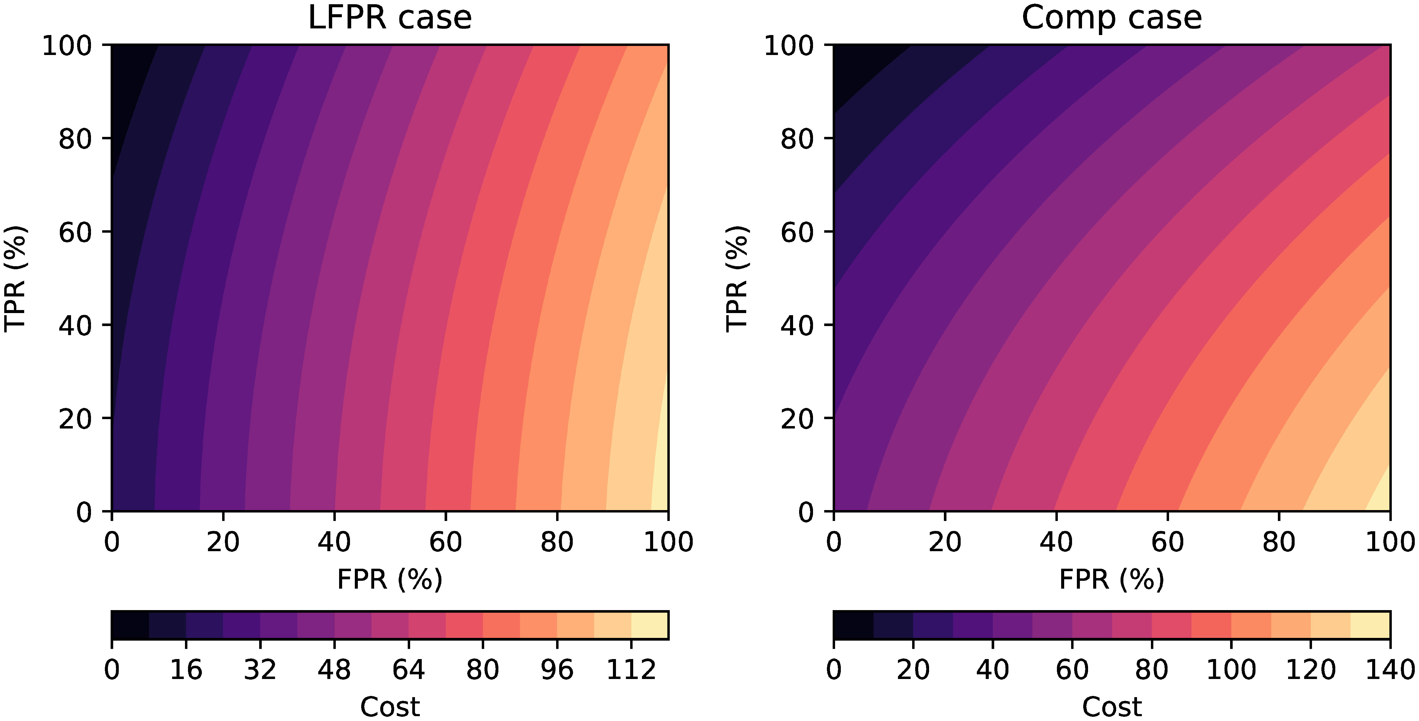
Figure 1 Values of the cost function used to generate optimal sets of QC checks in the LFPR and Comp cases.

The cost function is evaluated for each QC check from the first group defined above (location checks). Tests that fail to flag any profile or that flag all profiles are not considered. The test with the lowest cost function value is selected. For the LFPR case, the cost function value increases rapidly with FPR (Figure 1); therefore, QC checks that have a very low FPR tend to be selected. For the Comp case, the cost function contours are more sloped so QC checks that deliver a high TPR but moderate FPR might be selected over checks that have a very low FPR.

The cost function is then evaluated again, but for the combination of each check in the next group and the one already selected. The QC check which, when combined with the already selected test, gives the lowest cost function value is selected. As before, the cost functions will mean that QC checks with low FPR will tend to be selected for the LFPR case, but QC checks with strong improvements in TPR compared to the increase in FPR may be selected for the Comp case. The process is repeated until one from each group of QC checks is included. The algorithm will then add in other tests to the set if they meet two criteria. First, including the test must decrease the cost value of the set. Second, the TPR of the set must be increased by at least 1%. The second condition is used to avoid overfitting to the training data by adding QC checks that cause marginal decreases in the cost value but no significant improvement to the TPR.

2.1.5.2 HTPR case

The algorithm to find a set of quality control checks that aims to find as much of the bad data as possible (the HTPR case) is a two-phase process, beginning with a preprocessing step intended to reduce the space of tests and profiles under consideration. First, only QC tests with TPR/FPR > 2 were considered. This simple heuristic eliminates QC tests that don’t perform substantially better than arbitrarily assigning QC results. Also removed from consideration was any profile containing bad data not flagged by any QC test. These were set aside as objects of interest for potential future test development. As a final preprocessing step, any QC check which produced no false positives and at least one true positive flag was immediately accepted as a test which unambiguously flags undesirable features.

Once the preprocessing has reduced the tests and profiles under consideration, the main part of the HTPR algorithm is run on the set of remaining QC checks. This identifies tests that have high FPR and that can be removed from the set without reducing its overall TPR. By removing those tests from the set, it is possible achieve the highest possible TPR while remaining intolerant to false negatives. The procedure is as follows:

1) For every pair of QC tests, form a combination test by doing the logical AND of the QC results produced by the pair. The combination will only flag profiles that were rejected by both original tests, and therefore might be expected to produce a reduced number of false positives. Note that the code supports an arbitrary number of these combinations, for example ANDing together a combination with another combination, but in the interests of processing time the algorithm was run with pairs of single tests only.

2) The list of profiles that contain bad data according to the reference flags is examined to find any that were rejected by only one QC test or combination. The QC tests or combinations that flag those profiles are placed into a list of selected tests and then dropped from further consideration by the algorithm. In addition, all profiles that are flagged by those selected tests or combinations are dropped from further consideration. At this point in the algorithm, every profile that contains bad data and is still under consideration has been rejected by at least two QC tests. Therefore, it is possible to discard the QC test with the highest false positive rate without affecting the number of bad profiles that are being identified by the remaining QC tests. For example, if some of the profiles are all being rejected by two different checks on the gradients in the profiles, then we can safely discard whichever gradient check has the higher FPR since all the profiles are still being flagged by the other one.

These two steps are repeated in a loop until the set of accepted tests and combinations marks all profiles containing bad data.

2.1.6 QC flags

One of the QC sets could be applied to data by users to achieve their desired level of quality control. However, many users obtain their data from collections such as the IQuOD dataset (The IQuOD Team, 2018), which therefore needs to serve the needs of multiple users with different requirements. This is achieved here by assigning a QC flag of either 4, 3 or 2 to every level of each profile if the observation is rejected by the LFPR, Comp or HTPR QC set respectively. If more than one of the QC sets rejects the same observation, the highest number is used as the QC flag. If none of the sets reject the data, the QC flag is set to 1.

With this QC flag scheme it is possible to tell users which data have been rejected by each QC set. The QC flag value is also a simple to use indication of the level of confidence in the rejection of the data with 4 meaning the highest confidence and 2 the lowest confidence. A flag of 1 indicates that the data are expected to be good quality. This is similar to conventions in use internationally (Marine Environmental Monitoring and Prediction IOC, 2013). Users will often use only data with flags of 1 or 2 hence by default would reject data flagged by either the Comp or LFPR sets. However, with this scheme, users can choose to additionally use the HTPR flags if wished, or only reject the LFPR flagged data.

2.2 Data

Datasets with accurate QC information were required for this study. In addition, in order to successfully train and validate the checks, it was important that the datasets contain a broad spectrum of error modes and that the rejected data were retained in the profiles rather than discarded. These criteria limit the choice of datasets. The three datasets selected for use in this study are described in Sections 2.2.1 to 2.2.3.

2.2.1 QuOTA

The main dataset used in this study is the Quality-controlled Ocean Temperature Archive (QuOTA) (Gronell and Wijffels, 2008; Thresher et al., 2008, https://doi.org/10.25919/5ec357563bd3e). It was generated using AQC checks to identify suspect profiles, followed by manual quality control of those identified. The dataset was converted to the WOD ASCII format for the purpose of ingestion into the AutoQC software. A third of the data in QuOTA (January, February, March and June profiles) were entirely manually quality controlled when the dataset was originally created and these are used in this study. To avoid using profiles that had been added since the dataset was originally created, any profile outside the latitude-longitude range specified in Gronell and Wijffels (2008) was excluded. This was 70°S to the equator and 90°E to 145°E. In addition, profiles marked as duplicates were not used. This resulted in 47022 profiles in this dataset. Of these, 25932 (55%) were XBTs, 8862 (19%) were bottle/rosette/net observations, 8007 (17%) were mechanical bathythermographs (MBTs) and 3844 (8%) were from conductivity, temperature and depth (CTD) sensors. The remaining 1% consisted of 304 profiles from digital bathythermographs (DBTs), 56 from expendable CTDs (XCTDs), 4 from moored buoys and 13 unknown.

2.2.2 NOAA/AOML 100 profile set

This dataset, provided by the National Oceanic and Atmospheric Administration (NOAA) Atlantic Oceanographic and Meteorological Laboratory (AOML), consists of a manual selection of 100 XBT profiles obtained during actual XBT operations that are part of the Global XBT Network (Goni et al., 2019). These profiles were selected from 12 different geographical regions to include ocean features linked to specific dynamics and water mass properties in each of the following regions: North Atlantic, South Atlantic, Tropical Atlantic, North Pacific, South Pacific, Tropical Pacific, South Indian, Tropical Indian, Gulf of Mexico, Mediterranean Sea, high latitudes in the northern hemisphere, and high latitudes in the southern hemisphere. For each region, the NOAA/AOML profile set contains two good profiles and four bad profiles or profiles containing data points that should fail one or more tests, for example the test for spikes, possible rate of change, and climatology. Additionally, several good profiles were modified to introduce errors in the data and/or metadata in order to benchmark specific QC tests including impossible date, impossible location, location and maximum depth based on bathymetry, and maximum depth based on probe type. The data can be obtained from ftp://ftp.aoml.noaa.gov/phod/pub/bringas/XBT/AQC/AQC_IQUOD_2018/.

This dataset can be used to manually inspect the outputs produced by the quality control checks on profiles with known quality, and provides a straightforward way to determine the performance of different QC tests or methodologies. It was also prepared in order to assess the performance of different QC tests based on geographical region and the capacity of those tests to accurately account for rates of change in temperature or other profile structures associated with the ocean dynamics and variability of these regions.

2.2.3 Argo delayed mode data

The Argo project (Roemmich and Owens, 2000) launches autonomous profiling floats to primarily measure the temperature and salinity of the global ocean to 2000 m depth. Float variants include those that also make biogeochemical measurements and those that sample deeper in the ocean. Argo data are subjected to initial real time AQC and, later, delayed mode manual inspection (Wong et al., 2020a). Argo instruments collect profiles over a long time period and can be affected by sensor drifts (Wong et al., 2020b). It should be noted that the QC checks considered in this study are not designed to detect such drifts.

A year of Argo data (2010) was downloaded (data downloaded 30 September 2021) (Argo, 2021) and the delayed mode data run through the AutoQC system. The data are provided divided into Atlantic (30204 profiles), Indian (24803) and Pacific (56152) Ocean regions. This separation was retained in order to determine if there are regional variations in results.

3 Results

3.1 Pre-selected tests

The AutoQC system was run on the QuOTA dataset to generate quality control results for each profile. The results for the pre-selected tests are discussed here first.

During testing, visual inspection of profiles suggested that the CS wire break test may not function well for low resolution profiles because the depth levels are sufficiently far apart that the temperature change between levels is above the threshold set in the test. As the focus of this study is to use ‘off-the-shelf’ quality control algorithms as much as possible, tuning of the test to cope with this situation was not attempted. Instead, a simple approach was adopted where the QC decisions were ignored if all levels had been rejected. Following this modification, the numbers of profiles that contain rejects due to the pre-selected tests are listed in Table 2.

TABLE 2

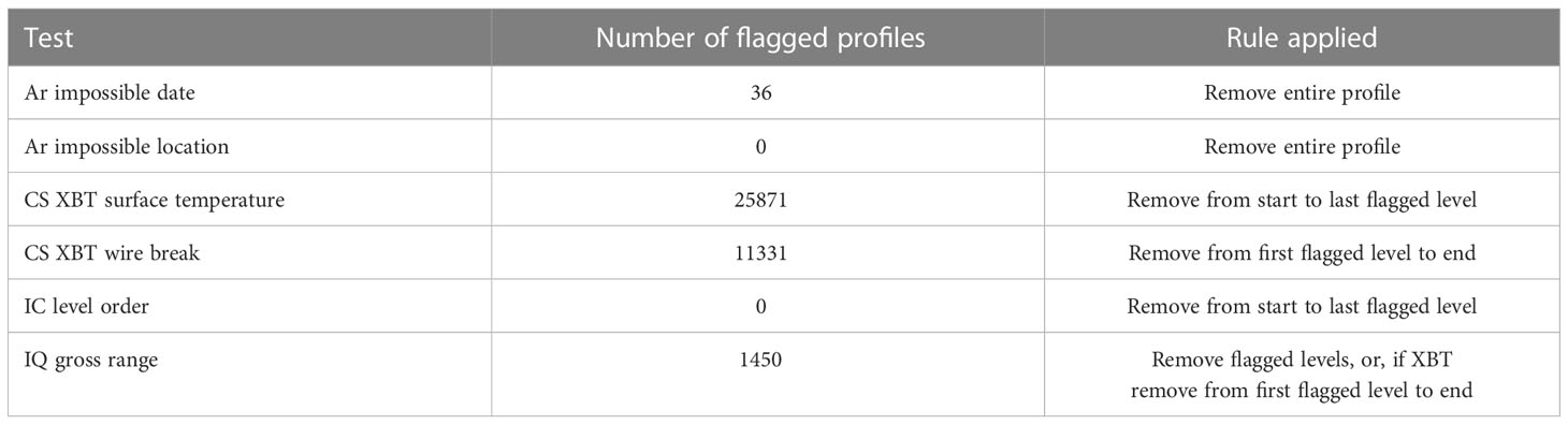
Table 2 Pre-selected QC checks, the number of profiles that they flag out of the 47022 profiles from the QuOTA dataset used in this study, and the rule applied to remove the affected data from the QuOTA dataset.

The outputs from the pre-selected tests were extracted and applied using the rule given in the table prior to running the training algorithms to select the best QC sets. For those tests that only flag part of a profile, two additional levels either side of a reject were also removed from the training data. This avoids the results from QC tests that use multiple levels in their algorithms from being contaminated by the data that were already rejected. Of the six selected, three reject zero or a very small number of profiles. The Ar impossible date and Ar location tests simply check that the date and location of the profile are sensible. For example a latitude of 95°N would be rejected by these tests. The ICDC (IC) level order check rejects levels with depths less than 0 m (i.e. above the surface of the water).

Of the three remaining pre-selected tests, the IQ gross range check results in the lowest number of flags applied to the profiles (3% of the total). The other two reject at least one level in a large number of profiles: the CS XBT surface temperature test (55%) and the CS XBT wire break test (24%). As the names imply, these two tests are only applied to XBT data. The former applies a manual QC procedure to reject XBT levels shallower than 3.6 m, because near-surface XBT data are unreliable due to the time lag in the thermistor response (Reseghetti et al., 2007). In QuOTA and XBT data quality controlled within Australia, these surface temperature values were replaced with 99.99 (Bailey et al., 1994; Gronell and Wijffels, 2008). As described in Section 2.1.2.2, the CS XBT wire break test is unique in the QC checks included in this study in attempting to detect that error mode specifically. However, as noted above, this test does not appear to work effectively for low vertical resolution profiles. Since the wire break manifests as an abrupt change in the recorded temperature at the deepest part of the profile, other tests (for example the spike or step checks) are also likely to be effective at finding these errors and may not be so sensitive to the profile’s vertical resolution.

From this point all statistics quoted refer to the data after application of the pre-selected QC tests and their associated rules.

3.2 Performance of individual tests

The pre-selected tests and their associated rules were applied to the QuOTA profiles and then the performance of the individual tests was calculated on the remaining data. These results are shown in Table 3 (non-bold text). The QC test that has the highest TPR (64.0%) is the second IC local climatology check, followed closely by the first version of this test (62.6%). The second IC local climatology check also has a better FPR than the first (12.7% versus 15.0%). The difference between these two IC local climatology checks is that the second check does not make an assumption on the statistical distribution of the data, which can cause outliers to be incorrectly identified as errors (Hubert and Vandervieren, 2008). Since this second check performs better than the first according to these results, it implies that asymmetrical thresholds can improve QC performance. Studying a different dataset and region, Castelão (2021) also suggested an asymmetry when comparing observations with WOA climatology. This illustrates the utility of benchmarking for demonstrating improvements in QC checks.

TABLE 3

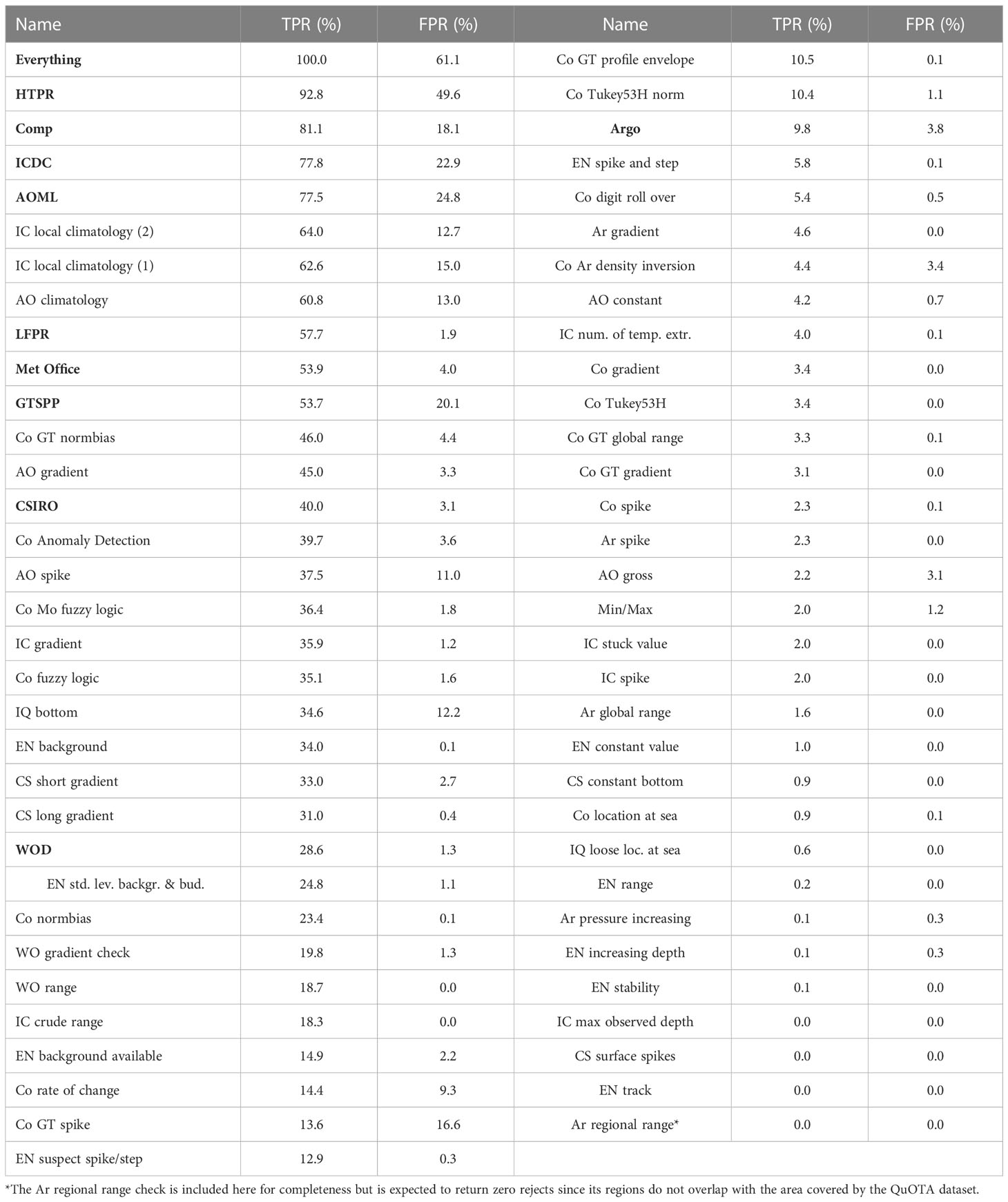
Table 3 TPR and FPR for individual QC checks (plain text) and combinations of checks (bold text) after removal of levels/profiles according to the pre-selected tests listed in Table 2.

The individual test with the third highest TPR is also a climatology check (AOML (AO) climatology). It has a slightly lower TPR (60.8%) and FPR (13.0%) than the IC versions, suggesting that the AO test is marginally more conservative in its rejection thresholds. Other background checks are considerably more conservative. For example, the FPR can be reduced to below 1% by using the EN background check if a lower TPR of 34.0% is accepted. Gradient, spike and range checks and the machine learning approach encapsulated in the CoTeDe (Co) Anomaly Detection test are also relatively successful at identifying profiles with bad data.

Increasing depth and stability checks are relatively ineffective types of tests according to these results. They reject proportionally similar or a greater percentage of profiles containing good data than those containing bad data. This is a surprising result for the increasing depth checks as these are simple algorithms to check that depths increase monotonically through the profile. This type of test was not used when generating QuOTA and this error mode was evidently not always flagged in the dataset. Both the Ar pressure increasing and EN increasing depth checks returned identical results. When generating combinations of tests, the EN increasing depth check was selected from the two since it employs a more sophisticated method of deciding which levels to reject. Stability checks rely on salinity information, which is not available for many profiles in the historical record. This can explain the poor performance of these checks, at least in part.

The EN track check failed to reject a significant number of profiles. It is likely that the QuOTA dataset is not well suited to benchmarking this test. In addition, the Ar regional range check only defines temperature ranges for the Red Sea and the Mediterranean Sea. This test therefore did not return any rejections since the QuOTA dataset contains no profiles in those seas.

3.3 Performance of combinations

The algorithms to find the best combination of checks were applied to the QuOTA data. As described in Section 2.1.5.1, the algorithm to find the Comp (to give a compromise between high TPR and low FPR) and LFPR (to give a low overall FPR) sets of checks employs a cost function to determine which QC checks are included. It is possible to vary the parameters that define the cost function (R₁ and R₂) to explore the range of possible results that might be obtained and to choose values for R₁ and R₂ to use for the LFPR and Comp cost functions. This was done, with both R parameters varied between 1 and 10 in steps of 0.25. Results are shown by small grey dots in Figure 2. A range of TPR and FPR rates were achieved, forming a curve with initially a steep increase in TPR as FPR increases to approximately 10%, then a slower rate of increase. The LFPR cost function settings were chosen as a point on the lower part of this curve where the FPR was less than 2% (cyan circle). Similarly, the values of R₁ and R₂ for the Comp case were selected by choosing a mid-point on the curve (red circle). In addition, the algorithm to obtain the HTPR (to give a high TPR) set of tests was run, resulting in the TPR and FPR shown by the black circle on Figure 2. The benchmarking results for the LFPR, Comp and HTPR sets are also given in Table 3.

FIGURE 2

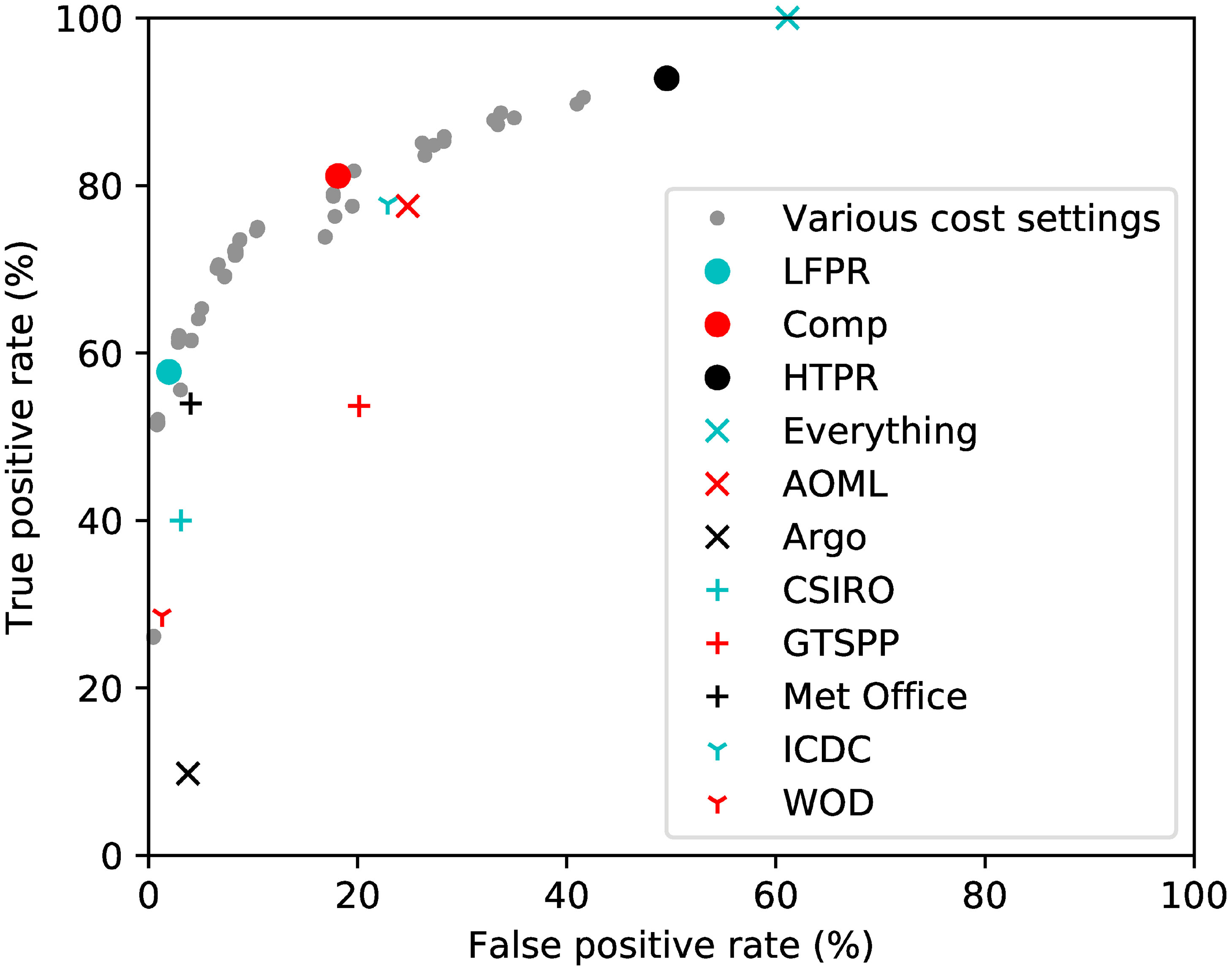
Figure 2 The TPR and FPR for each of the sets of QC tests, calculated from the full QuOTA dataset.

The QC checks included in the combinations are provided in Table 4. Pre-selected tests are also included in these combinations as these need to be run if applying the QC to datasets other than the QuOTA subset used here, which already had data rejected by those tests removed. The CS XBT wire break test was only inserted in the HTPR set given that, as discussed in Section 3.1, it may cause false positives when QCing low resolution profiles and because other QC checks included in the Comp and LFPR sets are expected to detect wire breaks. The CS XBT surface temperature test is included in the Comp and HTPR sets. This rejects all XBT data recorded at depths less than 3.6 m. The lack of inclusion in the LFPR set reflects that these shallow data may not be poor quality in all cases. The remaining pre-selected tests were inserted in all sets as there is high confidence in the rejections they provide. The order of the QC checks in the combinations follows the ordering of categories of tests defined in Section 2.1.5.1 and is the order in which they are recommended to be run. Within each QC set, where there was more than one test of the same type, the order in which the algorithms chose them is retained. The pre-selected tests and QC checks that do not fall into one of the categories of tests for which the ordering has been defined were ordered within the lists of tests according to the author’s expert judgement.

TABLE 4

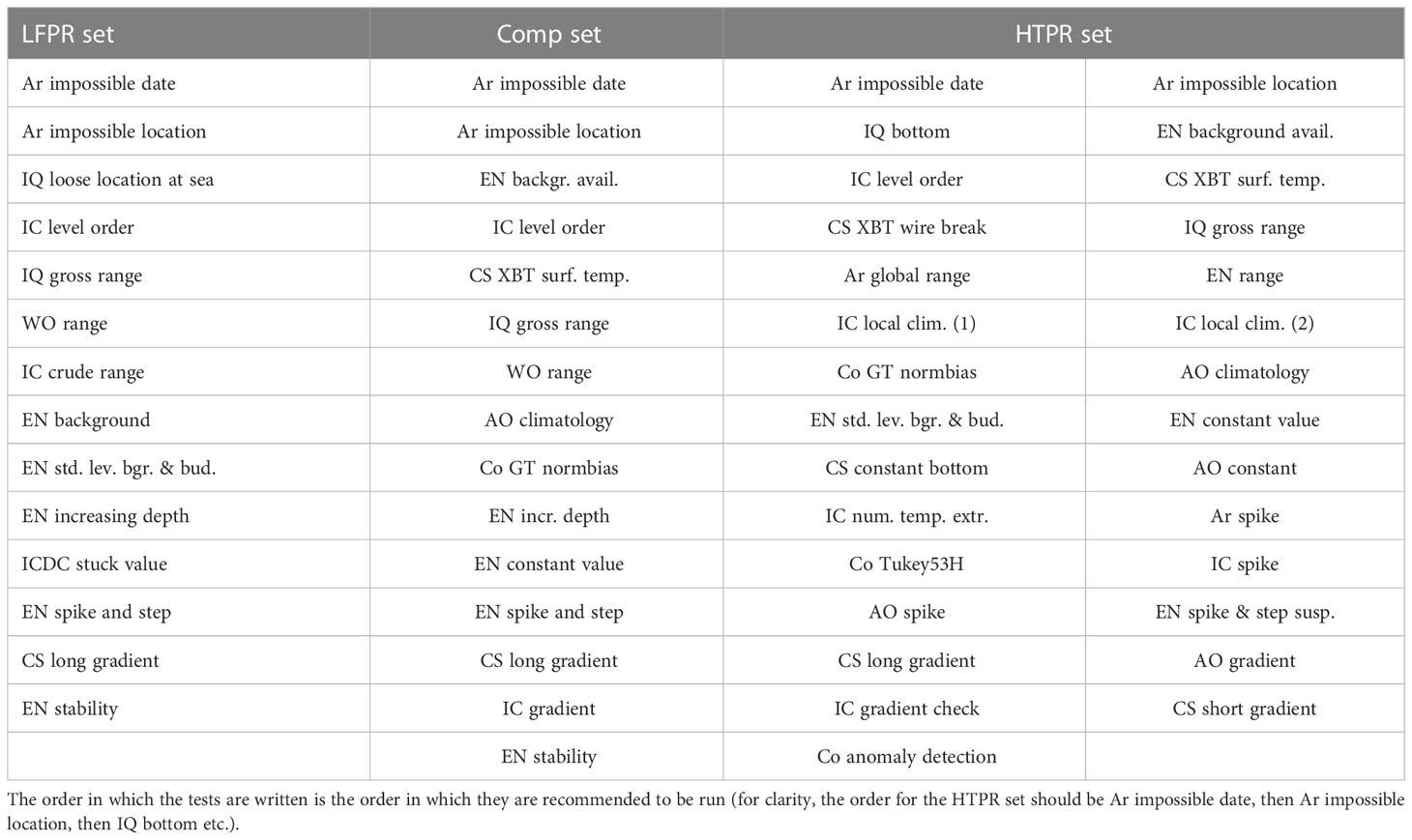
Table 4 IQuOD quality control sets.

Results for various other combinations of QC tests - for example all those from the ICDC set of checks - are also listed in Table 3 and shown in Figure 2. It should be noted that there are only two WOD checks included in the AutoQC repository and therefore these results are not necessarily representative of the WOD quality control procedures. The results show that the combination of tests run by different groups fall into two main categories. The first group provides moderate TPR (< 60%) with low FPR (<10%) and includes CSIRO, the Met Office and WOD. The second group has a higher FPR (>20%) but generally achieves better TPR than the first group. This group includes AOML and ICDC. The results suggest that the combination selection algorithms have worked effectively. The LFPR QC set achieves a higher TPR than the other sets in the first group of combinations, while the Comp set has a higher TPR and lower FPR than the second group. However, this is perhaps an unfair comparison since the algorithms were trained on the same data that are being used to validate them. Validation of the algorithm selection is described in Section 4.

By combining together all the QC checks included in the AutoQC repository (the ‘Everything’ set in Table 3), it is possible to flag every profile that contains bad data according to the reference flags; however, the FPR is 61.1%. This simple combination includes QC tests that are ineffective and flag a large number of profiles that should not contain rejects. The HTPR algorithm removes redundant and ineffective QC tests from the set of QC checks that are run, but still flags 92.8% of the bad profiles with a reduced FPR of 49.6%.

Figure 3 shows an example profile from the QuOTA dataset with the results from the different quality control sets shown using the QC flagging scheme described in Section 2.1.6.

FIGURE 3

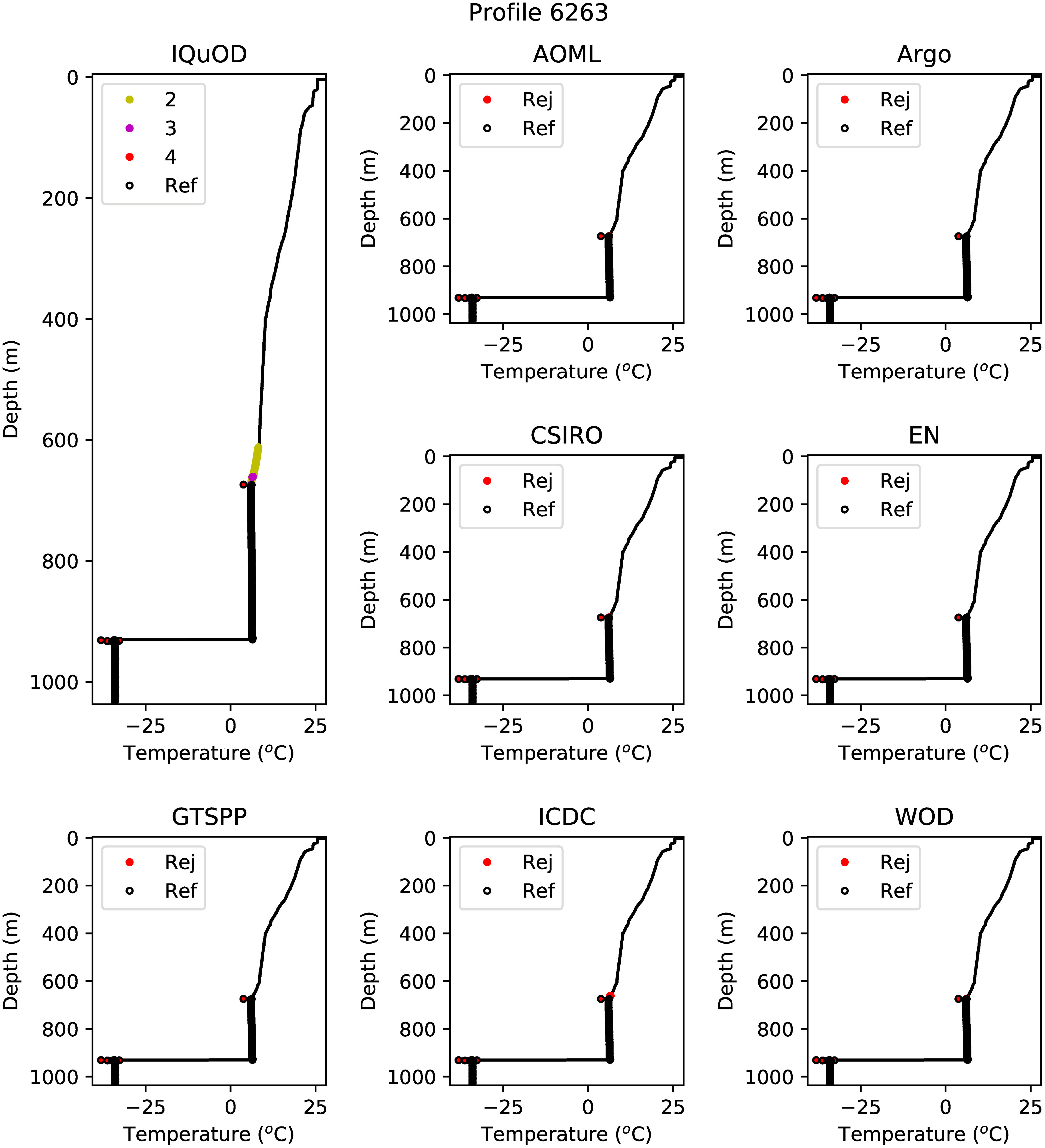
Figure 3 Example XBT profile from the QuOTA dataset. This was recorded on 23 March 1999 at 25.5167°S, 111.9167°E. For each set of QC results, the reference (‘Ref’) flags are shown by open black circles. Measurements rejected (‘Rej’) by the QC set are shown as filled red circles, except for the IQuOD QC sets derived in this study where the rejected measurements are assigned the number 2 (shown as a yellow filled circle), 3 (magenta) or 4 (red), with a higher number denoting increased confidence in the rejection.

4 Validation

4.1 Validation by subsetting QuOTA data

The algorithms that determined the quality control sets used the full QuOTA dataset. It is possible that the algorithms could overfit to the data and choose quality control checks that perform well on those data but less well on other sets. One way to assess this is to split the data into groups and use part for training and part for validation.

Two ways to subset the data have been tested: first, by dividing the data by instrument type, and second, by performing 10-fold cross-validation. The validation procedure involved assigning each profile to one of the subsets - in the former case the assignment was governed by the instrument type and in the latter case each profile was randomly assigned to one of ten subsets. Then, the data from all but one of the subsets were used to select QC sets and the results were validated on the remaining subset. This was repeated until all of the subsets had been used for validation. In addition, the QC sets derived from the entire QuOTA dataset were validated using each of the subsets.

4.1.1 Instrument type validation

As described in Section 2.2.1, over half of the QuOTA data used in this study are XBT profiles. Bottle/rosette/net, MBT and CTD profiles also make up a significant proportion of the dataset. The TPR and FPR of each individual QC check for the data from each of these types of data are shown in Figures 4A–D. In general, the QC checks perform best for XBT data - many have low FPR, with some of these having TPR in excess of 40%. In addition, a small number of the checks have TPR greater than 50% but with FPR still below 20% when applied to XBT data. Similar results are achieved for the CTD and bottle/rosette/net data, although there is more scatter in the points on the plot than for the XBTs. Results for MBT data are, however, much weaker, with only one QC check achieving greater than 40% TPR.

FIGURE 4

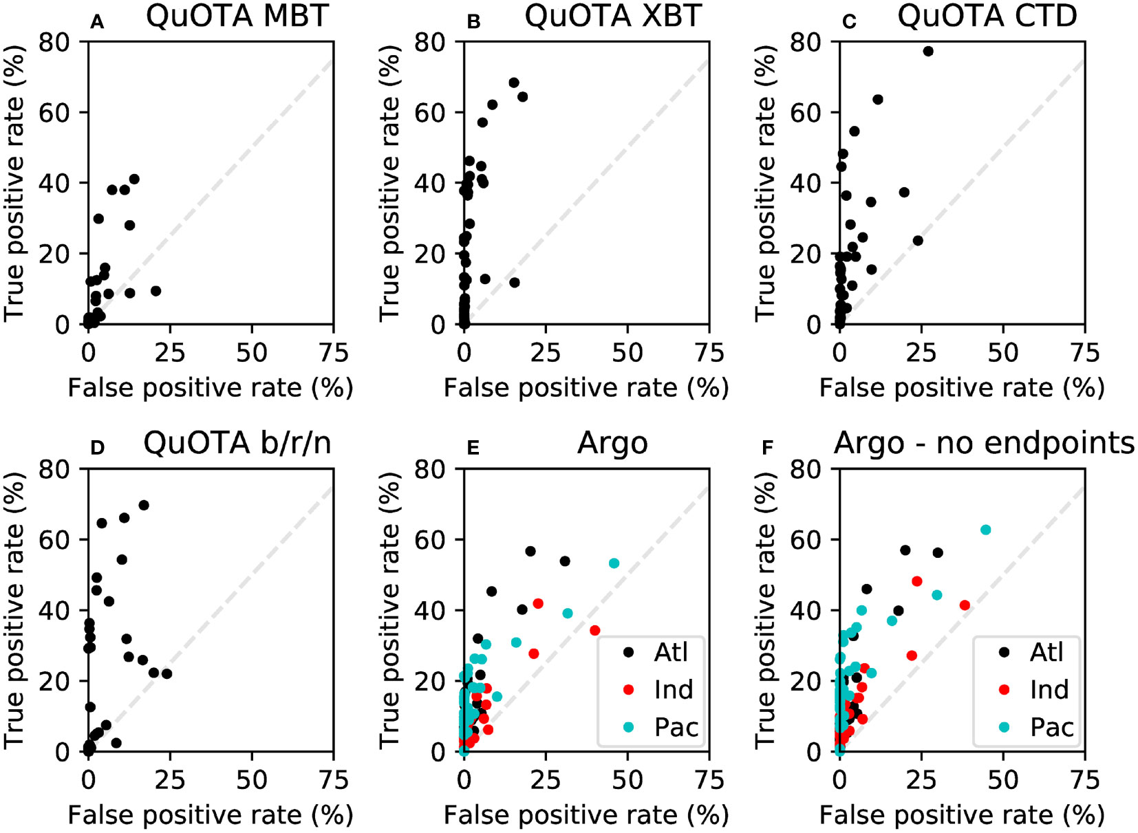
Figure 4 (A) The performance of each individual QC check on QuOTA MBT data; (B–D) as (A) except for QuOTA XBTs, CTDs and bottles/rosettes/nets respectively; (E) as (A) except for Argo profiles in 2010 for the Atlantic Ocean (Atl; blank circles), the Indian Ocean (Ind; red circles) and the Pacific Ocean (Pac; cyan circles); (F) as (E) but with the last profile point of each Argo profile removed. Grey dashes: the lines of equal TPR and FPR.

The performance of the LFPR, Comp and HTPR QC sets derived from the full QuOTA dataset on the data from each type of instrument is shown in Figure 5, top row. Results are shown as the difference to the TPR and FPR achieved for the full dataset. Results for XBT data (circles) are generally positive, with higher TPR and/or lower FPR than for the dataset as a whole, as might be expected given the strong results achieved by individual tests on the XBT data. For CTDs and bottle/rosette/net data, the LFPR case’s TPR is slightly lower than for the full dataset, the HTPR case’s FPR is slightly higher and a mixture of both occurs for the Comp case. Results for MBT data are poor, in particular for the LFPR and Comp cases, which reflects the performance of the individual tests on MBT data.

FIGURE 5

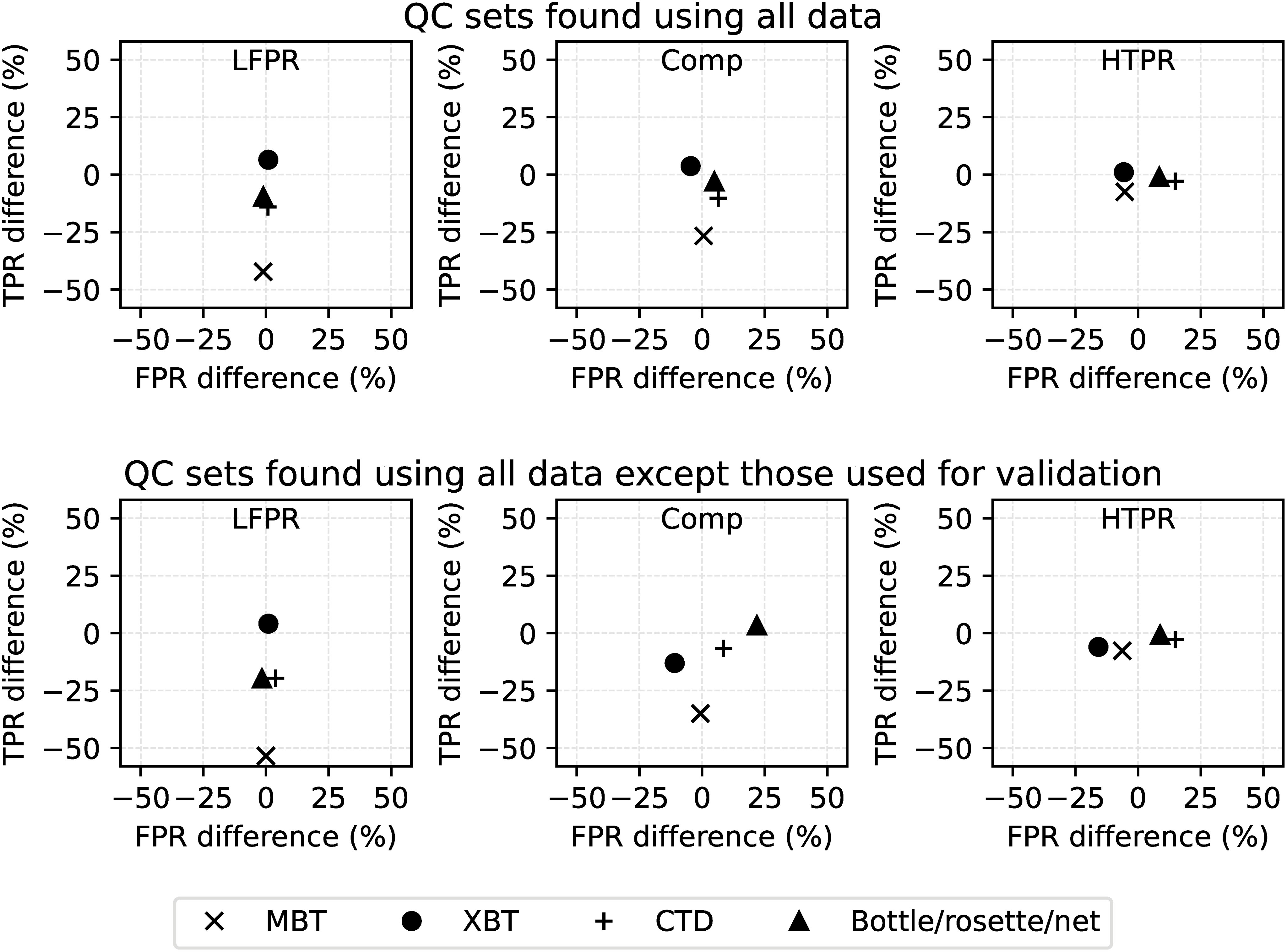
Figure 5 Top row: TPR and FPR calculated when applying the QC sets derived from the full QuOTA dataset to data from particular instrument types minus the TPR and FPR calculated from all the data; bottom row: as top row except the QC sets were derived from all data except those the TPR and FPR were calculated from.

Figure 5, bottom row, shows the results from generating the QC sets from all the data except those being used for the validation. This illustrates what might happen if using the QC sets obtained in this study on a data type that is not in QuOTA. For XBT data, the TPRs and FPRs obtained are either similar or both smaller than that from the full sets. Results for CTDs are similar to those obtained for QC sets found using all data. For the bottle/rosette/net data, the LFPR TPR is lower than when the training dataset included these data, and in the Comp case the FPR is larger. However, the HTPR results are similar. The TPR results for MBT data were poor for the LFPR and Comp cases.

In summary, the individual QC tests perform best on XBT data and poorly for MBT profiles. This poor performance for MBT data was reflected in the results for the LFPR and Comp QC sets, particularly when the MBT data were not included in the training dataset. However, the HTPR case was relatively robust to the type of data being QCed and whether the data type was included in the training dataset.

4.1.2 10-fold cross-validation

Figure 6 shows the results from performing the 10-fold cross-validation. As described above, this involved randomly assigning each profile to ten groups. Profiles from nine of the ten groups were used to select QC sets and these were validated on the data from the remaining group. This was repeated until all ten groups had been used for validation. Similar to Figure 5, the top row shows the TPR and FPR from applying the LFPR, Comp and HTPR QC sets to each of the ten subsets of the QuOTA data and the second row is the same but for the LFPR, Comp and HTPR sets derived from all the data except those in the subset being used to calculate the TPR and FPR. In all cases, the results are shown as the difference to the TPR and FPR obtained when applying the LFPR, Comp and HTPR QC sets derived from all the QuOTA data to the full dataset.

FIGURE 6

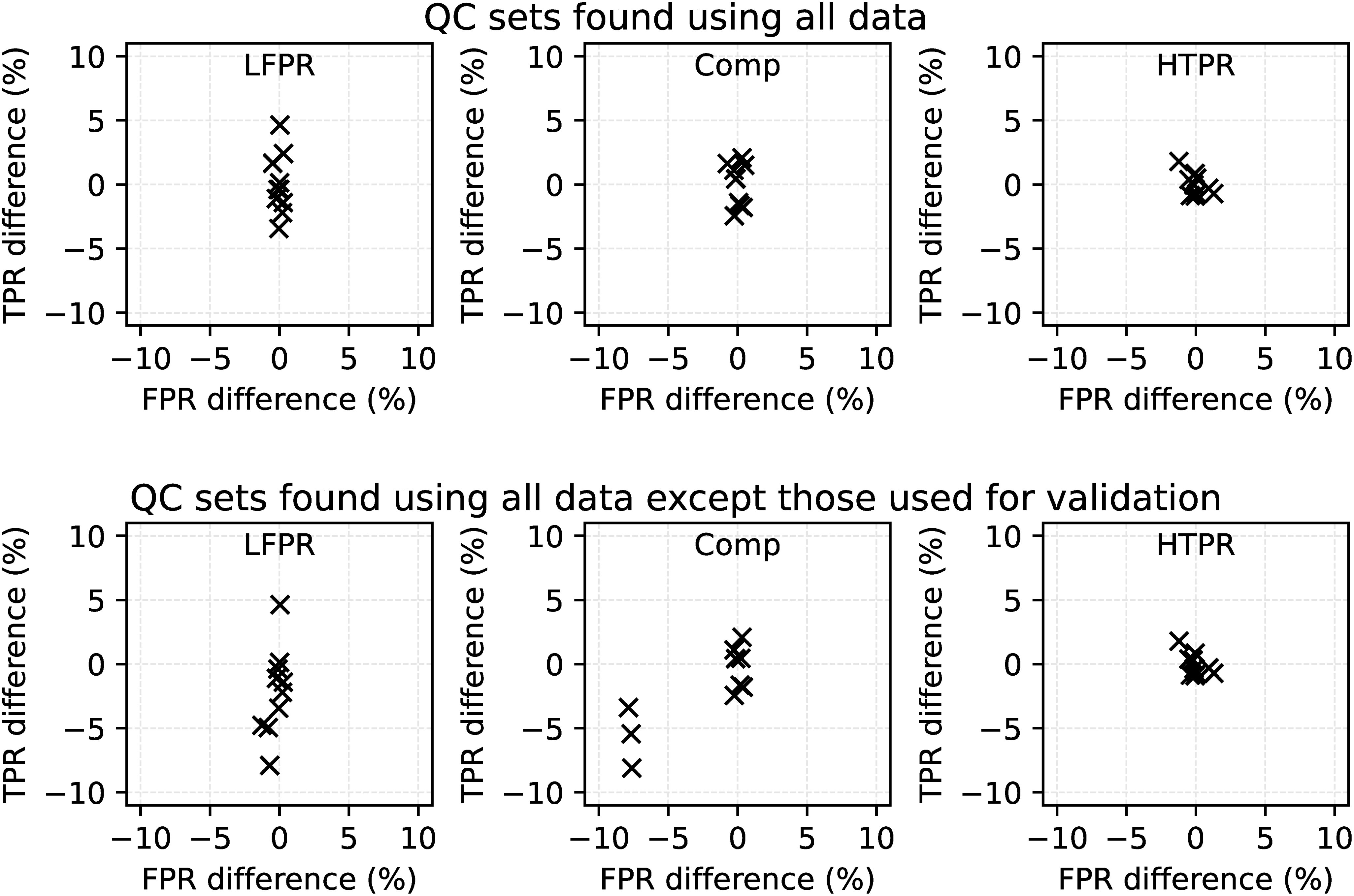
Figure 6 Top row: TPR and FPR calculated when applying the QC sets derived from the full QuOTA dataset to data from each subset minus the TPR and FPR calculated from all the data; bottom row: as top row except the QC sets were derived from all data except those the TPR and FPR were calculated from.

The largest variation in the TPRs occurs for the LFPR QC set. The differences tend to be negative (i.e. the TPR is worse than when applying the QC sets to all the QuOTA data), particularly when the QC sets were derived from data that excluded the subset used to calculate the TPR and FPR. However, the variation is relatively small compared to that found for different data types in Section 4.1.1.

In general, the results for the Comp and HTPR QC sets show relatively little variation in TPR and FPR. The exception is for three of the subsets for the Comp case, in the situation where the QC sets were found from data not in those subsets. Examination of the QC sets obtained for these three cases revealed that a different selection of QC sets had occurred. For example, the AO climatology check was not selected in those sets, but was in the others. Table 5 details the frequency with which particular QC tests were selected in a QC set. Bold numbers denote that a test was also in the QC sets derived from the full QuOTA dataset. The selection of tests was, in general, very stable, and many of the tests included in the sets obtained from all the QuOTA data were also selected with every instance of the subsetted data.

TABLE 5

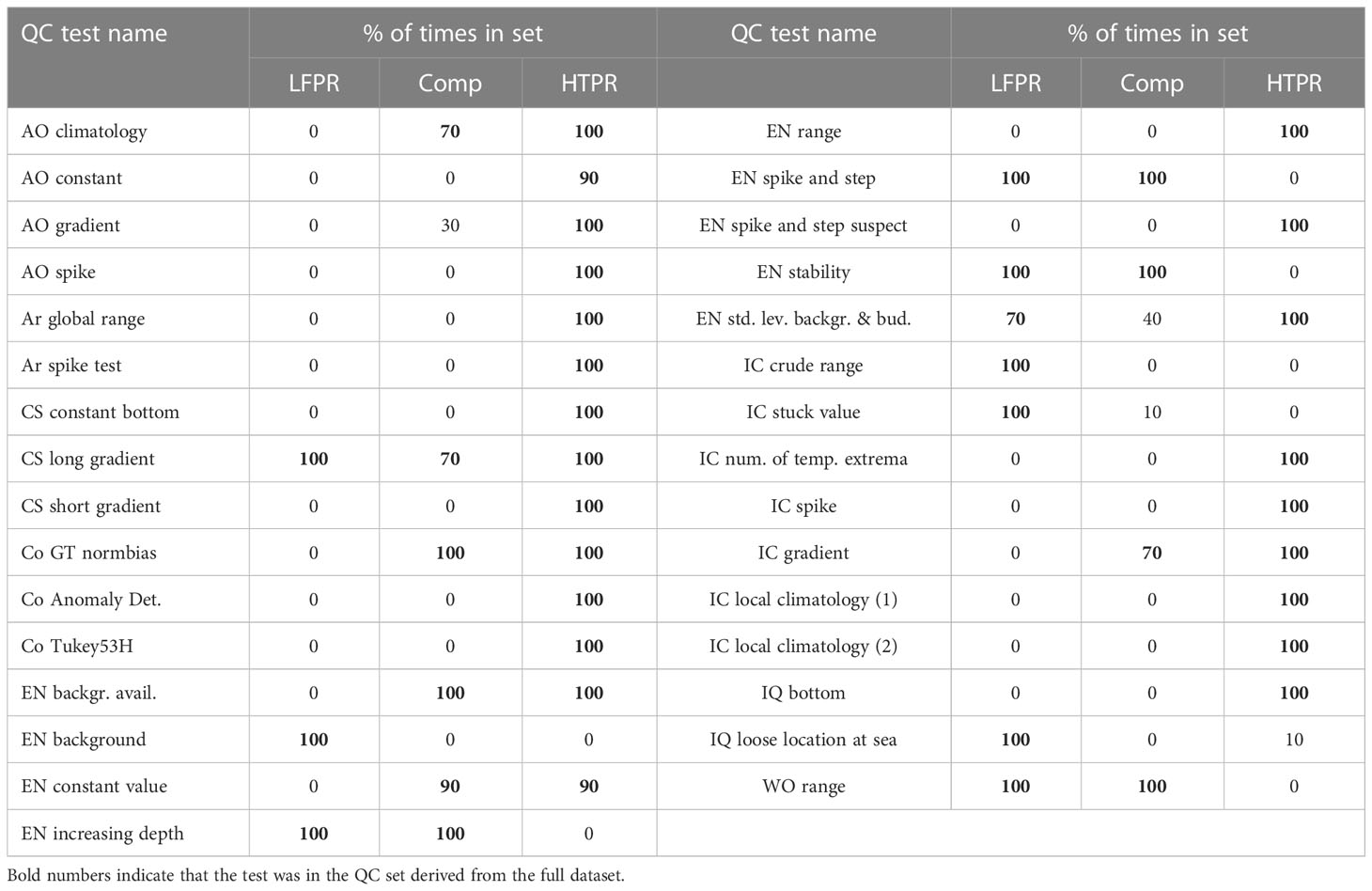
Table 5 Percentage of times each test appears in the QC sets derived in the 10-fold cross-validation.

4.2 Validation using the NOAA/AOML 100 XBT profile dataset

The NOAA/AOML dataset of profiles and the results obtained by applying the QC tests to them were examined to provide an overall qualitative assessment of the ability of the QC sets to detect the errors in the profiles. It was found that, in general, the QC sets derived in this study perform well. An example of a profile from the NOAA/AOML dataset (Figure 7) shows that the IQuOD QC sets derived in this study have successfully rejected the poor quality data below approximately 550 m. Other QC sets have varying success in flagging these data with some QC sets not detecting the spikes at all (Argo and EN sets) and some partially detecting them (e.g. GTSPP and WOD). The full NOAA/AOML dataset of profiles is shown in the supplementary material.

FIGURE 7

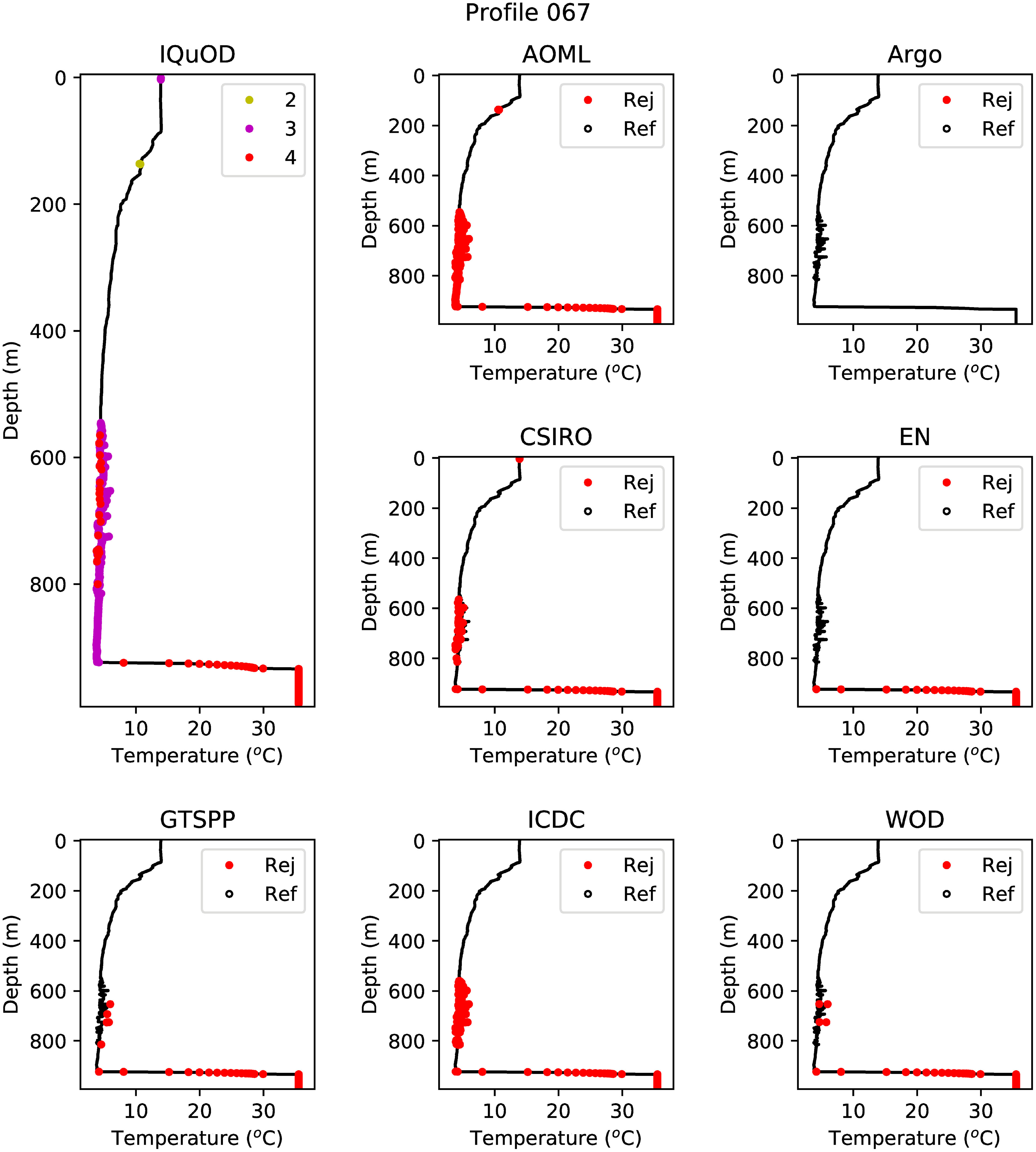
Figure 7 As Figure 3 except for an example profile from the NOAA/AOML dataset. This profile is from the South Atlantic Ocean at 43.500°S and 40.886°W and has a time stamp of 1 September 2017. It shows many spikes between 550 m and 850 m.

4.3 Validation using Argo delayed mode data

The benchmarking statistics calculated for the Argo data are shown in Table 6. The results from the QuOTA dataset after the pre-selected tests were applied are also included for comparison. The Argo dataset contains a similar proportion of profiles containing flagged data as QuOTA (13.6 - 17.2% compared to 14.0% for QuOTA). The performance of each individual QC test is shown in Figure 4E. The majority of tests achieve TPR < 30%. Of those that achieve higher TPR, the results for the Atlantic Ocean are better overall than those for the Indian and Pacific Oceans. In the latter cases the results are close to the dashed grey lines in the plots, which shows the line of equal TPR and FPR. The TPR achieved by the QC sets (Table 6) is in all cases lower in the Argo results than in the QuOTA results, particularly for the Indian Ocean. FPR is similar in the LFPR case but higher in the Comp and HTPR cases.

TABLE 6

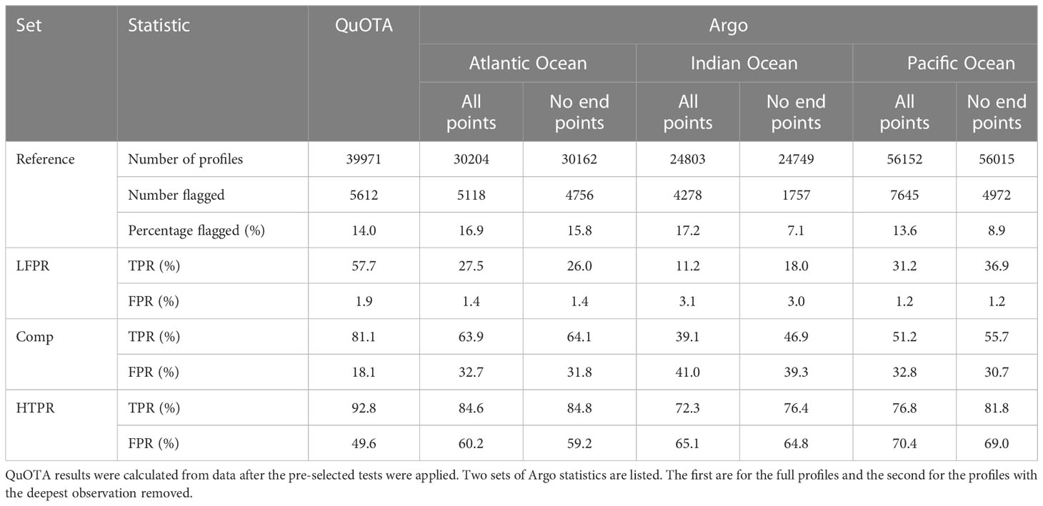
Table 6 TPR and FPR for the QuOTA dataset and each of the Argo regional datasets.

Inspection of Indian and Pacific Ocean profiles identified that the deepest level of the profile is often flagged in the delayed mode Argo quality control for these regions. Figure 8 shows an example profile containing this feature. These rejections are likely associated with the occurrence of ‘salinity hooks’ at the base of Argo profiles caused by water from the surface or parking level remaining in the conductivity sensor at the start of measuring the profile (Wong et al., 2020a). Therefore, results were also generated when disregarding this level. This made a significant difference to the number of profiles rejected in the reference QC flags for the Indian and Pacific Oceans (Table 6), with the rejection rate for the Indian Ocean reduced from 17.2% to 7.1% and for the Pacific Ocean from 13.6% to 8.9%. There was also a noticeable improvement in the results for the individual QC tests (Figure 4F). However, while the TPRs achieved by the QC sets were also improved for the Indian and Pacific basins (Table 6), it was not sufficient to bring the results into agreement with those from the QuOTA data.

FIGURE 8

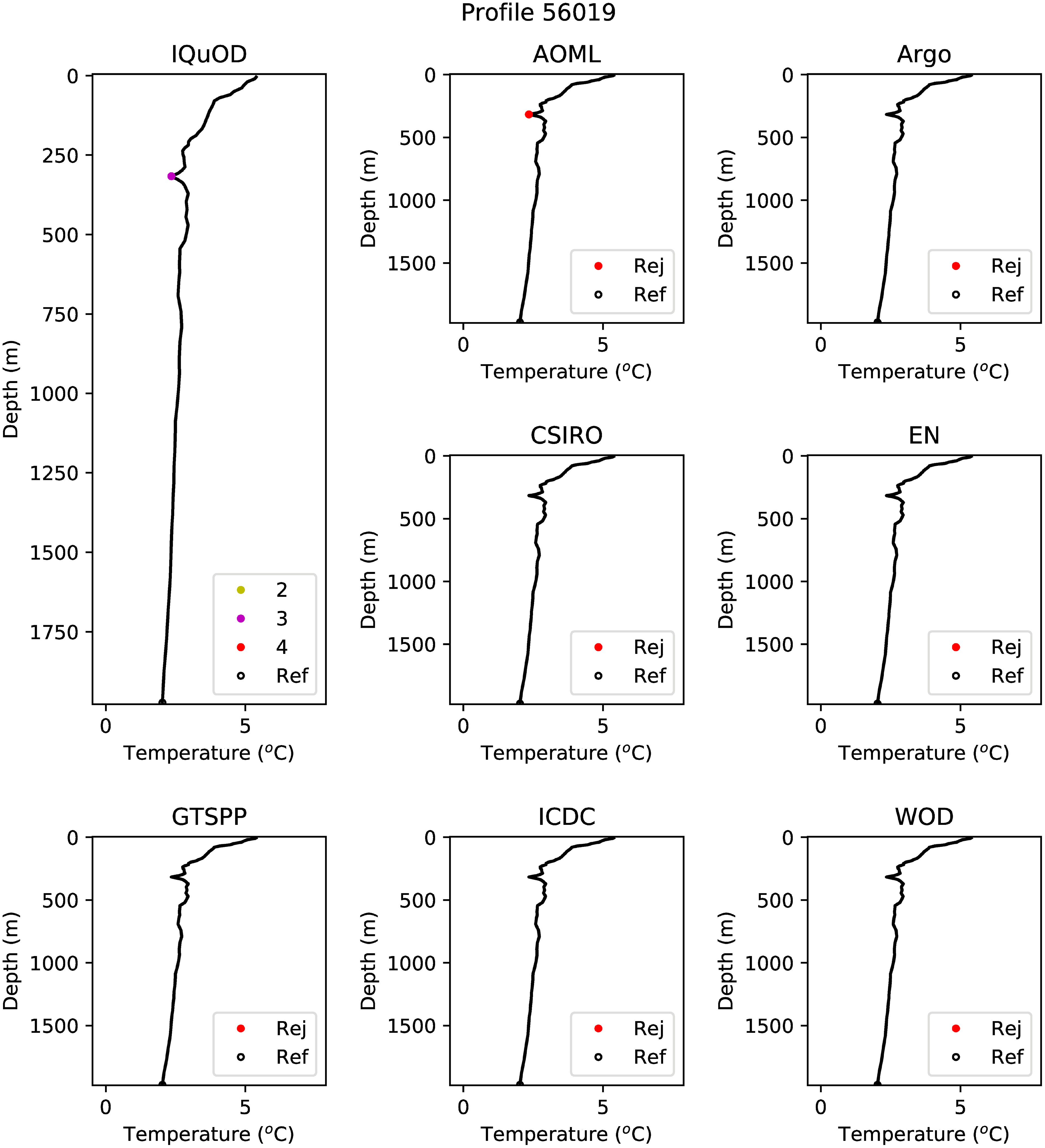
Figure 8 As Figure 3 except for an example Argo profile - number 56019 in the data analyzed for the Pacific Ocean - at 57.344°S, 170.453°E on 29 December 2010.

Figure 9 shows a comparison of the benchmarking results for different quality control sets for the Atlantic Ocean, Pacific Ocean and Indian Ocean data after removal of the deepest level. A number of the QC sets including Argo (which would be expected to work effectively on these data), the Met Office and the LFPR set are successful at flagging a relatively small proportion of profiles with Argo delayed mode rejections. The Met Office and LFPR results are very similar. Inspection of the results suggests this is due to both sets including the EN background and EN increasing depth checks. Compared to the Argo QC set, the Met Office and LFPR have a higher TPR but also a non-zero FPR rate. The LFPR QC could therefore be a useful alternative to the Argo real time QC if a higher TPR is desirable and loss of some good data is acceptable. At the other end of the scale, the HTPR set flags 76.4 - 84.8% of the rejected profiles but also 59.2 - 69.0% of those without reference flags. Applying all QC tests achieved a similar result to the HTPR set. The Comp, AOML, GTSPP and ICDC sets lie between the two other groups.

FIGURE 9

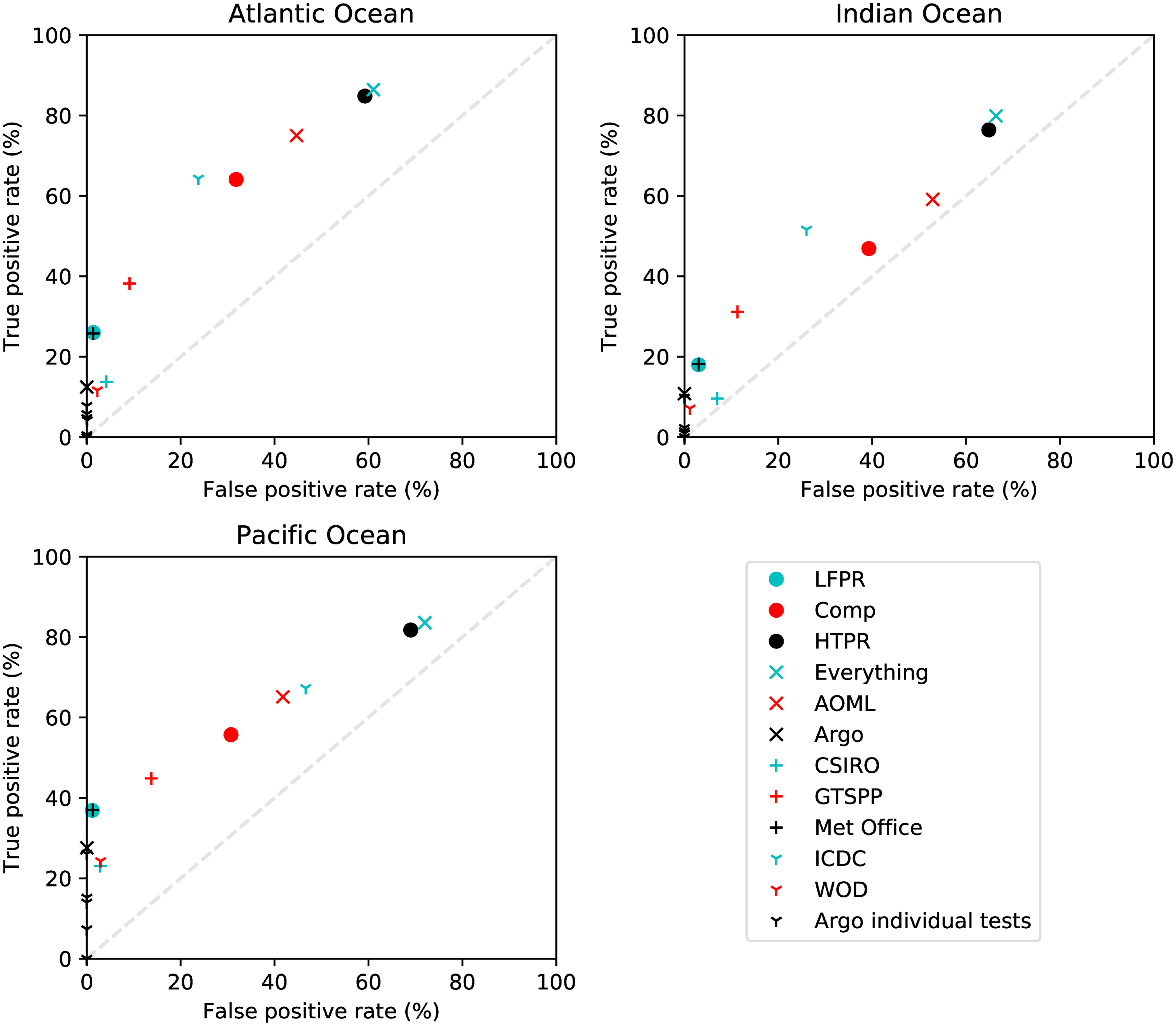
Figure 9 TPRs and FPRs for different QC sets calculated from delayed mode Argo data in the Atlantic, Indian and Pacific ocean regions. End points of profiles were removed before generating the results. The results for individual Argo QC tests are also shown including the Min/Max test as this was designed for application to Argo data. A line showing equal TPR and FPR is drawn to aid comparison of results.

Underlying these results is that the individual QC tests have significantly different TPRs and FPRs than assessed using QuOTA. For example the AO climatology test, which has a TPR of 60.8% and FPR of 13.0% according to the QuOTA data, has, for example, a TPR of 56.2% and FPR of 30.0% from the Atlantic Ocean Argo data, 44.3% and 29.7% in the Pacific Ocean and for the Indian Ocean they are 41.4% and 38.2%. The regions covered by the QuOTA data and the Indian Ocean Argo data are the most similar so it is perhaps surprising that the greatest difference in TPR and FPR occurs there. The regional variability could suggest that the test works better in some regions than others, or that the Argo delayed mode QC may vary, or both could be a factor.

A concern with the results shown in Figure 9 is that the different quality control sets approximately lie on a line with gradient of 1 (i.e. parallel to the dashed grey line shown in the plots). This implies that there is little correlation between the profiles that are being flagged and the Argo reference flags because for every additional 1% of profiles with Argo flagged data that are rejected by the QC sets, 1% of the profiles with no Argo flagged data are also rejected. It is likely the case that there are error modes that occur in the Argo data that the AQC checks are not detecting. The QC checks may also not be optimized for the high quality Argo data, and may be better suited to the types and frequency of error modes that occur in instruments such as XBTs. The individual Argo QC checks (including the Min/Max test, which was derived using CTD datasets (Argo, ship-board CTD, mammal-mounted CTD) (Gourrion et al., 2020b)), all have very low FPR (Figure 9), which may therefore be a design choice, but this may not be a good choice if quality controlling data from instruments that are more prone to problems.

Figure 8 shows an Argo profile where one of the levels was rejected by the QC checks but not in the delayed mode flags. It is difficult to design tests that do not reject the types of features shown while still finding genuine errors. It highlights that it should not be taken for granted that quality control checks that are effective for one type of data will work for another type. In the future, this may mean designing or optimizing tests for each type of data and it also highlights the need for human QC operators in addition to automatic checks.

5 Discussion

In this study, various AQC checks for temperature profile data used by the international scientific community have been benchmarked using a subset of the QuOTA dataset that had previously been subjected to manual QC. As well as showing which checks perform best according to the benchmarks, QC test sets have been identified that provide better FPR and/or TPR than those being run by individual organizations and qualitatively perform well on the NOAA/AOML curated set of 100 profiles with known characteristics. The QC checks included in those sets were shown to be robust when deriving and validating the sets using 10-fold cross-validation. Larger differences occurred when validating by dividing the data by instrument type, with the QC performing best on XBT data but worst on MBT data. Performance was also lower than for QuOTA when applying the QC sets that try to achieve a high or moderate TPR to Argo delayed mode data, which may reflect differences in the types of error modes that occur in Argo data compared to other data types and the need for manual QC to identify some of these. However, it was noted that Argo AQC checks have very low FPR and the QC set that attempts to minimize false positives was found to be comparatively effective on Argo data, albeit while providing a lower TPR than achieved on QuOTA.

The results highlight the need for training data representative of the various errors that occur in the datasets that the QC tests are being applied to. A crucial aspect of this is knowing the reason why a manual QC operator has rejected particular data. A simple example of this was found with the Argo delayed mode data. It was found that in many cases the last level of an Argo profile is rejected, despite no obvious discrepancies with the level above in the temperature profile. This type of rejection is specific to Argo delayed mode data and hence is not seen in the QuOTA profiles. Knowledge of this might allow an AQC check to be implemented and, if there was more than one implementation, to include some of these data in the reference dataset and benchmark them.

In the future, the hope is to create a virtuous circle within the IQuOD project where manual QC is performed on a selection of profiles. The operator will be able to mark the reason for a rejection. This could then become an expanding dataset for training AQC and machine learning techniques (which can themselves be benchmarked in the AutoQC system), covering all regions rather than the restricted latitude/longitude range of QuOTA. Knowledge of which errors are not being identified by the AQC could lead to new tests being developed or to improvements in already-implemented tests. It will therefore be possible to improve the overall quality of the full dataset faster than would be possible if trying to manually QC all profiles. Automatic techniques should also be useful in detecting which profiles would benefit most from manual QC. Machine learning (such as used for the Co Anomaly Detection test (Castelão, 2021)) is expected to become increasingly valuable in the future and the benchmarking provided by the AutoQC system will be very useful to track progress in this work.

Refinements are also possible in the way the QC checks included in AutoQC are implemented. For example, the checks are currently set up as independent tests. All QC tests process the full dataset and in the few cases where QC checks rely on information from another (for example EN background uses outputs from EN spike and step suspect), this is dealt with by calling the other routines from within the code for that check or using saved outputs within the SQLite dataset. In other systems, such as WOD (Garcia et al., 2018), QC checks are run in a particular order and rejected data removed so that later checks do not have to deal with problems that are already detected. This can allow the later tests to be more sensitive to the errors they are designed to find. A version of this approach has been implemented in the IQuOD QC sets through use of expert judgement. Improvement to the order in which QC tests are run was one of the recommendations of Tan et al. (2022) and with a controlled test dataset containing known errors it would be possible to do focused studies to determine the benefits from a defined processing order. Another refinement would be to apply expert judgements to the way that levels within a profile are rejected. The example of which levels around a spike should be rejected was given earlier. A second example is for XBT data, where the convention is that if a wire break is found all levels deeper are also deemed suspect and should be given the same flag. Third, experts might recommend particular tests or thresholds for different regions or instrument types.

The benchmarking framework that has been set up has, so far, been used only for temperature profile data. However, there are other essential ocean (climate) variables, such as salinity, for which QC is also crucial. The same benchmarking techniques can be applicable to those physical variables.

In summary, the benchmarking and QC sets discussed in this paper are intended to be a first iteration. In the future, the integration of AQC, machine learning QC and manual QC under the IQuOD project will enable a framework where each aspect can improve the other, iteratively improving the quality of the full temperature profile dataset in the future, and eventually extending the techniques to other variables.

6 Conclusions

As part of the IQuOD project, open source software infrastructure was developed to benchmark sixty AQC checks for ocean temperature profile data and to determine the best set of tests. The software was coded in Python and is publicly available under the MIT license. Algorithms were also developed to determine the optimal sets of quality control checks. The software was applied to profiles from the QuOTA dataset to which manual QC had been applied by the dataset developers, and therefore there was high confidence that the quality of the data was known. Three set of checks were derived, which allowed the identification of as much suspect data as possible at the cost of rejecting potentially good data (the HTPR set), to only flag the most suspect data with the cost of missing some data which should have been rejected (the LFPR set), or a compromise between the two (the Comp set).

The set selections have been validated by subselecting the training data and using two independent datasets. Results from the subselecting were relatively consistent with the original results when 10-fold cross-validation was applied. They were less consistent when the dataset was split by instrument type, with the best results for XBT profiles and worst for MBT profiles. The results of applying the tests to a curated set of 100 XBT profiles developed by NOAA/AOML were qualitatively satisfactory. When applying the QC to delayed mode Argo data, the Comp and HTPR sets derived from the QuOTA training data did not perform well. However, the LFPR set performed satisfactorily when compared to the Argo real time QC procedures but achieved a lower TPR than that calculated for the QuOTA data. This result was not confined to the sets determined in this study – the individual tests and groups of quality control checks used by different data producers around the world were similarly affected. This highlights that quality control performance can vary according to the data being processed. It is recommended that the underlying causes of these differences are investigated in the future.

The QC sets found in this study will be used to QC historical data that have not previously had extensive QC applied such as XBTs and will be released by the IQuOD project from a NOAA portal (current version is available at https://doi.org/10.7289/v51r6nsf) (The IQuOD Team, 2018). The three IQuOD sets of QC checks will be applied separately to the dataset with a QC value of 1 assigned to data that are not rejected by any of the sets, 2 to data that are rejected by only the HTPR set of checks, 3 if the Comp set rejects the data but not the LFPR set, and 4 if the LFPR set returns a reject. For appropriate QC tests, it is also recommended that XBT data deeper than a rejection flag are marked with the same flag. Users can choose to (i) use only data with a flag value of 1, which excludes all data identified by the QC sets as being suspect, (ii) use data with QC flags of 1 or 2, which provides a balance between finding as much bad data as possible without rejecting too much good data, or (iii) use data with QC flags of 1, 2 of 3, which will mean that the only data that are rejected are those where there is high confidence that they are bad. If it is unclear to the user which to use, the recommendation is to use data with flag values of 1 or 2 and reject data with flag values of 3 or 4.

It is expected that this dataset and the new understanding of the performance of QC methods obtained in this study will serve to improve forecasting, reanalysis and monitoring of the state of the ocean. This study is seen as a first step. In the future, the software infrastructure that has been set up will foster more effective and timely advances in AQC evaluations (e.g. inclusion of other checks, either existing or newly developed), through coordination of international expertise and resources into a best practice community effort. The aim is to facilitate evolving AQC activities and data refinements (along with full documentation) in support of the highest quality and most consistent global temperature profile database. In addition, the overall AQC framework can serve as a template for enhancing the quality of other essential climate variables (ECVs), such as ocean salinity, and their value to scientific and societal applications.

Data availability statement

The raw data supporting the conclusions of this article will be made available by the authors, without undue reservation.

Author contributions

SG lead writing of the manuscript; BM and SG were the main code developers; SG ran the software to generate the results; TB performed data conversion; FB and GG conceptualized and produced the NOAA/AOML dataset; GC contributed to the code and wrote and provided expertise on the CoTeDe software; RC provided expertise and information on the QuOTA dataset and CSIRO QC checks; VG provided information and ancillary data that enabled the ICDC checks to be used; CMD reviewed and edited the manuscript; all authors were involved in discussing and shaping the work and contributed to the manuscript. All authors contributed to the article and approved the submitted version.

Funding

This work was supported by the Scientific Committee on Oceanic Research (SCOR) Working Group 148, funded by national SCOR committees and a grant to SCOR from the U.S. National Science Foundation (OCE-1840868). IQuOD is a project of the International Oceanographic Data and Information Exchange (IODE) programme of the Intergovernmental Oceanographic Commission of UNESCO, and they also supported this work. NOAA/AOML and the NOAA GOMO Program supported GG and FB. RC was supported with funding from the Australian Government under the National Environmental Science Program. VG was supported by the Strategic Priority Research Program of the Chinese Academy of Sciences (Grant no. XDB42040402) and National Natural Science Foundation of China (Grant no. 42076202). CMD was supported by the Natural Environment Research Council NE/P019293/1.

Acknowledgments

Argo data were collected and made freely available by the International Argo Program and the national programs that contribute to it. (http://www.argo.ucsd.edu, http://argo.jcommops.org). The Argo Program is part of the Global Ocean Observing System. We thank Ann Gronell Thresher, whose work on the QuOTA dataset and the initial iteration of AQC benchmarking in IQuOD inspired this work, the entire IQuOD team for their useful inputs, comments and suggestions, and Patrick Halsall for preparing Python versions of the AOML QC code on which the AutoQC implementations were based. We also thank the two reviewers for their useful comments, which improved the manuscript.

Conflict of interest

The authors declare that the research was conducted in the absence of any commercial or financial relationships that could be construed as a potential conflict of interest.

Publisher’s note

All claims expressed in this article are solely those of the authors and do not necessarily represent those of their affiliated organizations, or those of the publisher, the editors and the reviewers. Any product that may be evaluated in this article, or claim that may be made by its manufacturer, is not guaranteed or endorsed by the publisher.

Supplementary material

The Supplementary Material for this article can be found online at: https://www.frontiersin.org/articles/10.3389/fmars.2022.1075510/full#supplementary-material

References

Argo (2021). Argo float data and metadata from global data assembly centre (Argo GDAC) SEANOE. doi: 10.17882/42182

CrossRef Full Text | Google Scholar

Bailey R., Gronell A., Phillips H., Tanner E., Meyers G. (1994). Quality control cookbook for XBT data (Expendable bathythermograph data). Version 1.1. (Australia: CSIRO Marine Laboratories Report: 221), 37. doi: 10.25607/OBP-1482

CrossRef Full Text | Google Scholar

Balmaseda M., Hernandez F., Storto A., Palmer M., Alves O., Shi L., et al. (2015). The ocean reanalyses intercomparison project (ORA-IP). J. Operat Oceanog. 8, s80–s97. doi: 10.1080/1755876X.2015.1022329

CrossRef Full Text | Google Scholar

Bellucci A., Gualdi S., Masina S., Storto A., Scoccimarro E., Cagnazzo C., et al. (2013). Decadal climate predictions with a coupled OAGCM initialized with oceanic reanalyses. Clim Dyn 40, 1483–1497. doi: 10.1007/s00382-012-1468-z

CrossRef Full Text | Google Scholar

Blockley E. W., Martin M. J., McLaren A. J., Ryan A. G., Waters J., Lea D. J., et al. (2014). Recent development of the Met Office operational ocean forecasting system: An overview and assessment of the new Global FOAM forecasts. Geosci. Model. Dev. 7, 2613–2638. doi: 10.5194/gmd-7-2613-2014

CrossRef Full Text | Google Scholar

Boyer T., Baranova O., Coleman C., Garcia H., Grodsky A., Locarnini R., et al. (2018). World Ocean Database 2018. Ed. Mishonov A. V., Technical Editor (NOAA, Silver Spring, MD. NOAA Atlas NESDIS), 87.

Google Scholar

Bushnell M., Waldmann C., Seitz S., Buckley E., Tamburri M., Hermes J., et al. (2019). Quality assurance of oceanographic observations: Standards and guidance adopted by an international partnership. Front. Mar. Sci. 6. doi: 10.3389/fmars.2019

CrossRef Full Text | Google Scholar

Cabanes C., Grouazel A., von Schuckmann K., Hamon M., Turpin V., Coatanoan C., et al. (2013). The CORA dataset: validation and diagnostics of in-situ ocean temperature and salinity measurements. Ocean Sci. 9, 1–18. doi: 10.5194/os-9-1-2013

CrossRef Full Text | Google Scholar

Castelão G. (2020). A framework to quality control oceanographic data. J. Open Source Soft. 5, 2063. doi: 10.21105/joss.02063

CrossRef Full Text | Google Scholar

Castelão G. (2021). A machine learning approach to quality control oceanographic data. Comput. Geosci. 155, 104803. doi: 10.1016/j.cageo.2021.104803

CrossRef Full Text | Google Scholar

Chassignet E. P., Hurlburt H. E., Metzger E. J., Smedstad O. M., Cummings J. A., Halliwell G. R., et al. (2009). US GODAE: Global ocean prediction with the HYbrid Coordinate Ocean Model (HYCOM). Oceanography 22, 64–75. doi: 10.5670/oceanog.2009.39

CrossRef Full Text | Google Scholar

Cowley R., Killick R. E., Boyer T., Gouretski V., Reseghetti F., Kizu S., et al. (2021). International Quality-controlled Ocean Database (IQuOD) v0.1: The temperature uncertainty specification. Front. Mar. Sci. 8. doi: 10.3389/fmars.2021.689695

CrossRef Full Text | Google Scholar

Domingues C. M., Palmer M. D. (2015). The IQuOD initiative: towards an international Quality Controlled Ocean Database. CLIVAR Exchanges 67 (19), 38–40.

Google Scholar

Dong J., Domingues R., Goni G., Halliwell G., Kim H.-S., Lee S.-K., et al. (2017). Impact of assimilating underwater glider data on Hurricane Gonzalo, (2014) forecasts. Weather Forecast. 32, 1143–1159. doi: 10.1175/WAF-D-16-0182.1

CrossRef Full Text | Google Scholar

Dunstone N. J., Smith D. M. (2010). Impact of atmosphere and sub-surface ocean data on decadal climate prediction. Geophysical research letters 37. doi: 10.1029/2009GL041609

CrossRef Full Text | Google Scholar

ETOP05 (1988). Data announcement 88-MGG-02, digital relief of the surface of the earth (Boulder, Colorado: NOAA, National Geophysical Data Center).

Google Scholar

Garcia H. E., Boyer T. P., Locarnini R. A., Baranova O. K., Zweng M. M. (2018). World Ocean Database 2018: User’s manual (prerelease). Mishonov A. V. Technical Ed., (NOAA, Silver Spring, MD). Available at: https://www.ncei.noaa.gov/products/world-ocean-database.

Google Scholar

Goni G. J., Sprintall J., Bringas F., Cheng L., Cirano M., Dong S., et al. (2019). More than 50 years of successful continuous temperature section measurements by the global expendable bathythermograph network, its integrability, societal benefits, and future. Front. Mar. Sci. 6. doi: 10.3389/fmars.2019.00452

CrossRef Full Text | Google Scholar

Good S. A., Martin M. J., Rayner N. A. (2013). EN4: Quality controlled ocean temperature and salinity profiles and monthly objective analyses with uncertainty estimates. J. Geophys. Res.: Oceans 118, 6704–6716. doi: 10.1002/2013JC009067

CrossRef Full Text | Google Scholar

Good S., Mills B. (2022). AutoQC: Automatic quality control analysis for the International Quality Controlled Ocean Database. Zenodo. doi: 10.5281/zenodo.5832003

CrossRef Full Text | Google Scholar

Gouretski V. (2018). World ocean circulation experiment – argo global hydrographic climatology. Ocean Sci. 14, 1127–1146. doi: 10.5194/os-14-1127-2018

CrossRef Full Text | Google Scholar

Gouretski V., Koltermann K. (2004). WOCE global hydrographic climatology: A technical report Vol. 35 (Hamburg, Germany: Bundesamtes für Seeschiffahrt und Hydrographie).

Google Scholar

Gourrion J., Dobler D., Gallian M., Szekely T., Beaulieu N. (2020a). Reference files and python code to run Min/Max QC test. SEANOE doi: 10.17882/77199

CrossRef Full Text | Google Scholar

Gourrion J., Szekely T., Killick R., Owens B., Reverdin G., Chapron B. (2020b). Improved statistical method for quality control of hydrographic observations. J. Atmospheric Oceanic Technol. 37, 789–806. doi: 10.1175/JTECH-D-18-0244.1

CrossRef Full Text | Google Scholar

Gronell A., Wijffels S. E. (2008). A semiautomated approach for quality controlling large historical Ocean Temperature Archives. J. Atmospheric Oceanic Technol. 25, 990–1003. doi: 10.1175/JTECHO539.1

CrossRef Full Text | Google Scholar

Gulev S., Thorne P., Ahn J., Dentener F., Domingues C., Gerland S., et al. (2021). Changing state of the climate system. In Climate Change 2021: The physical science basis. Eds. Masson- Delmotte V., Zhai P., Pirani A., Connors S. L., Péan C., Berger S., Caud N., Chen Y., Goldfarb L., Gomis M. I., Huang M., Leitzell K., Lonnoy E., Matthews J. B. R., Maycock T. K., Waterfield T., Yelekçi O., Yu R., Zhou B. (Cambridge, United Kingdom and New York, NY, USA: Cambridge University Press), 287–422. doi: 10.1017/9781009157896.004

CrossRef Full Text | Google Scholar

Haddad S., Killick R. E., Palmer M. D., Webb M. J., Prudden R., Capponi F., Adams S. V. (2022). Improved infilling of missing metadata from expendable bathythermographs (XBTs) Using multiple machine learning methods. Journal of Atmospheric and Oceanic Technology. 39(9), 1367–1385.

Google Scholar

Hubert M., Vandervieren E. (2008). An adjusted boxplot for skewed distributions. Comput. Stat Data Anal. 52, 5186–5201. doi: 10.1016/j.csda.2007.11.008

CrossRef Full Text | Google Scholar

Ingleby B., Huddleston M. (2007). Quality control of ocean temperature and salinity profiles - historical and real-time data. J. Mar. Syst. 65, 158–175. doi: 10.1016/j.jmarsys.2005.11.019

CrossRef Full Text | Google Scholar

Johnson G. C., Lyman J. M., Boyer T., Cheng L., Domingues C. M., Gilson J., et al. (2019). Southern Ocean [in State of the Climate in 2018]. Bull. Amer. Meteor. Soc. 100, S74–S77. doi: 10.1175/2019BAMSStateoftheClimate.1

CrossRef Full Text | Google Scholar

King R. R., Lea D. J., Martin M. J., Mirouze I., Heming J. (2020). The impact of Argo observations in a global weakly coupled ocean-atmosphere data assimilation and short-range prediction system. Q. J. R. Meteorol. Soc. 146, 401–414. doi: 10.1002/qj.3682

CrossRef Full Text | Google Scholar

King R. R., While J., Martin M. J., Lea D. J., Lemieux-Dudon B., Waters J., et al. (2018). Improving the initialisation of the Met Office operational shelf-seas model. Ocean Model. 130, 1–14. doi: 10.1016/j.ocemod.2018.07.004

CrossRef Full Text | Google Scholar

Laloyaux P., de Boisseson E., Balmaseda M., Bidlot J.-R., Broennimann S., Buizza R., et al. (2018). CERA-20C: A coupled reanalysis of the twentieth century. J. Adv. Model. Earth Syst. 10, 1172–1195. doi: 10.1029/2018MS001273

CrossRef Full Text | Google Scholar

Lellouche J.-M., Greiner E., Le Galloudec O., Garric G., Regnier C., Drevillon M., et al. (2018). Recent updates to the Copernicus Marine Service global ocean monitoring and forecasting real-time 1/12° high-resolution system. Ocean Sci. 14, 1093–1126. doi: 10.5194/os-14-1093-2018

CrossRef Full Text | Google Scholar

Locarnini R. A., Mishonov A. V., Baranova O. K., Boyer T. P., Zweng M. M., Garcia H. E., et al. (2019). World Ocean Atlas 2018, volume 1: Temperature. A. Mishonov Technical Ed Vol. 81 (NOAA Atlas NESDIS), 52 pp.

Google Scholar

Marine Environmental Monitoring and Prediction IOC (2013). “Recommendation for a quality flag scheme for the exchange of oceanographic and marine meteorological data,” in Ocean data standards, vol. 3. (Paris, France: UNESCO-IOC) 54 (3), 5pp. doi: 10.25607/OBP-6

CrossRef Full Text | Google Scholar

Mills B., Castelão G., Good S., Winsemius R. (2017). IQuOD/wodpy: 1.5.0 (Zenodo). doi: 10.5281/zenodo.839253

CrossRef Full Text | Google Scholar

Morello E. B., Galibert G., Smith D., Ridgway K. R., Howell B., Slawinski D., et al. (2014). Quality control (QC) procedures for Astralia’s National Reference Station’s sensor data – comparing semi-autonomous systems to an expert oceanographer. Methods Oceanog. 9, 17–33. doi: 10.1016/j.mio.2014.09.001

CrossRef Full Text | Google Scholar

Palmer M. D., Boyer T., Cowley R., Kizu S., Reseghetti F., Suzuki T., et al. (2018). An algorithm for classifying unknown expendable bathythermograph (XBT) instruments based on existing metadata. J. Atmospheric Oceanic Technol. 35, 429–440. doi: 10.1175/JTECH-D-17-0129.1

CrossRef Full Text | Google Scholar

Penny S. G., Akella S., Balmaseda M. A., Browne P., Carton J. A., Chevallier M., et al. (2019). Observational needs for improving ocean and coupled reanalysis, S2S prediction, and decadal prediction. Front. Mar. Sci. 6. doi: 10.3389/fmars.2019.00391

CrossRef Full Text | Google Scholar

Reseghetti F., Borghini M., Manzella G. M. R. (2007). Factors affecting the quality of XBT data – results of analyses on profiles from the Western Mediterranean Sea. Ocean Sci. 3, 59–75. doi: 10.5194/os-3-59-2007

CrossRef Full Text | Google Scholar

Roemmich D., Owens W. B. (2000). The Argo project: Global ocean observations for understanding and prediction of climate variability. Oceanography 13, 45–50. doi: 10.5670/oceanog.2000.33

CrossRef Full Text | Google Scholar

Schiller A., Brassington G. B., Oke P., Cahill M., Divakaran P., Entel M., et al. (2020). Bluelink ocean forecasting Australia: 15 years of operational ocean service delivery with societal, economic and environmental benefits. J. Operat Oceanog. 13, 1–18. doi: 10.1080/1755876X.2019.1685834

CrossRef Full Text | Google Scholar

Schmidtko S., Johnson G. C., Lyman J. M. (2013). MIMOC: A global monthly isopycnal upper-ocean climatology with mixed layers. J. Geophys. Res.: Oceans 118, 1658–1672. doi: 10.1002/jgrc.20122

CrossRef Full Text | Google Scholar

Storto A., Alvera-Azcárate A., Balmaseda M. A., Barth A., Chevallier M., Counillon F., et al. (2019). Ocean reanalyses: Recent advances and unsolved challenges. Front. Mar. Sci. 6. doi: 10.3389/fmars.2019.00418

CrossRef Full Text | Google Scholar

Tan Z., Zhang B., Wu X., Dong M., Cheng L. (2022). Quality control for ocean observations: From present to future. Sci. China Earth Sci. 65, 215–233. doi: 10.1007/s11430-021-9846-7

CrossRef Full Text | Google Scholar

The IQuOD Team (2018). International Quality Controlled Ocean Database (IQuOD) version 0.1 - aggregated and community quality controlled ocean profile data 1772-present NOAA National Centers for Environmental Information. Dataset. doi: 10.7289/v51r6nsf

CrossRef Full Text | Google Scholar

Thresher A., Cowley R., Wijffels S. (2008). QuOTA dataset (Quality-controlled Ocean Temperature Archive) v3. CSIRO. Data Collection. doi: 10.25919/5ec357563bd3e

CrossRef Full Text | Google Scholar

UNESCO-IOC (2010). “GTSPP real-time quality control manual, first revised edition,” in United Nations educational, scientific and cultural organization, vol. 7. (Paris: Place de Fontenoy), 75352.

Google Scholar

von Schuckmann K., Traon P.-Y. L., (Chair) N. S., Pascual A., Djavidnia S., Gattuso J.-P., et al. (2019). Copernicus Marine service ocean state report, issue 3. J. Operat Oceanog. 12, S1–S123. doi: 10.1080/1755876X.2019.1633075

CrossRef Full Text | Google Scholar

Wong A., Keeley R., Carval T.,, Argo Data Management Team (2020a). Argo quality control manual for CTD and trajectory data. doi: 10.13155/33951

CrossRef Full Text | Google Scholar

Wong A. P. S., Wijffels S. E., Riser S. C., Pouliquen S., Hosoda S., Roemmich D., et al. (2020b). Argo data 1999–2019: Two million temperature-salinity profiles and subsurface velocity observations from a global array of profiling floats. Front. Mar. Sci. 7. doi: 10.3389/fmars.2020.00700

CrossRef Full Text | Google Scholar

Zuo H., Balmaseda M., Mogensen K. (2017). The new eddy-permitting ORAP5 ocean reanalysis: Description, evaluation and uncertainties in climate signals. Clim Dyn 49, 791–811. doi: 10.1007/s00382-015-2675-1

CrossRef Full Text | Google Scholar