Impact of assimilating repeated subsurface temperature transects on state estimates of a western boundary current

1 Introduction

Subtropical Western Boundary Currents (WBCs) are narrow, rapidly flowing warm water currents that are important for ecosystems, climate, weather and cross-shelf exchange (e.g. Lambaerts et al., 2013; Malan et al., 2020; Oliver et al., 2021; Li et al., 2022a). As fast-flowing WBC jets become unstable, they shed O(100) km-wide mesoscale eddies. The formation, structure and evolution of these eddies and associated structures are important due to the impact they have on the transport of heat and salt (Abernathey and Haller, 2018), weather (Frenger et al., 2013), mixing (Klocker and Abernathey, 2014), and the delivery of nutrients (Everett et al., 2012).

Given their location adjacent to populous coastlines, WBCs have a pivotal role in coastal fisheries and other blue economies (e.g. Young et al., 2011; Brieva et al., 2015), weather and climate, and search-and-rescue and navigation. An impediment to manyof these end-users is the limitation in model predictability resulting from the dynamically changing eddy field. Mesoscale dynamics are inherently sensitive, where divergent evolution results from small differences in initial conditions. This leads to a timescale limit on predictability for techniques such as search and rescue, navigation and other methods that require accurate forecasts of ocean weather.

Accurate estimates and predictions of WBCs and eddy-rich regions are generally sought through data-assimilating models (Oke et al., 2013). The technique of data assimilation combines observations with a model forecast, often in an iterative process, to produce an analysis or optimal estimate of the ocean state. Hence, the evolution of eddies can be continually updated within model forecasts, providing a best estimate of eddy structure, timing and location (Oke et al., 2013).

One of the key ways in which operational forecasting systems differ from non-operational, research-focussed assimilation systems is the types of observations that can be assimilated. For example, operational forecast systems typically assimilate sea surface height (SSH), sea surface temperature (SST), a smaller number of subsurface observations, such as vertical temperature profiles from expendable bathythermograph (XBT) probes and Argo floats, as well as occasionally wind stress and sea surface salinity observations (e.g. Brassington et al., 2007).

In contrast, hindcast reanalyses with a research focus (e.g. Kerry et al., 2016; Siripatana et al., 2020), can augment these traditional observation types with more novel, often delayed-mode observations, e.g. high frequency radar-inferred surface currents, hydrography from autonomous gliders, and measurements from subsurface moorings. The constraint limiting operational forecast systems from assimilating the full gamut of non-traditional and subsurface observations, is the ability to have data prepared and available in near-real time for the next operational window — which can often not be met when quality control or other data preparation must be conducted with human supervision, or obviously if there is a delay in data recovery. As a result, operational systems will often be limited to just surface observations combined with a small number of near-real time subsurface measurements.

The East Australian Current (EAC; see Figure 1 for region) is one such WBC with routine subsurface sampling. The EAC flows southwards from 27.5°S as a coherent jet, before beginning to meander and lose coherency between 31°–33°S and then feeding an ‘evolving’ field of cyclonic and anticyclonic eddies in the Tasman sea. Like many other WBCs, an important source of subsurface real-time measurements in the EAC are repeated XBT transects and Argo floats. A long-term program of XBT deployments from ships of opportunity has been operated along repeat transects in the southern Pacific Ocean since the late 1980s (and 1991 for the two transects through the EAC region, named ‘PX30’ and ‘PX34’) by Scripps Institution of Oceanography, the Australian Commonwealth Scientific and Industrial Research Organisation and the New Zealand National Institute for Water and Atmospheric Research. The original use of this data was for estimating boundary current heat budgets (e.g. Roemmich and Cornuelle, 1990; Morris et al., 1996; Roemmich et al., 2005). However the near-real time data delivery and consistent transects lends itself well to data assimilation into ocean models. As the XBT data is delivered to the global telecommunications system it is readily available in near realtime for ingestion into operational modelling systems and reanalyses (e.g. Carton et al., 2000).

Argo floats are a second source of subsurface observations that have also been used in operational forecasting. Argo floats return vast amounts of deep (to 2000 m) vertical temperature and salinity profiles over a much broader area of the ocean and have revolutionised understanding of the ocean (Wijffels et al., 2016; Wong et al., 2020). However, they still have relatively low spatial distribution and are not measuring systematically e.g. along repeat transects at routine time and space scales. Thismeans the data cannot easily be used for closed box heat budgets, their Lagrangian paths could lead to sample aliasing, nor can we systematically assess observation impact. For these reasons we do not consider Argo data in this analysis.

It has been shown with data assimilation experiments that weekly subsurface temperature (XBT-like) observations have a significant impact on representation of the EAC: improving mean surface and subsurface circulation patterns, upper ocean heat content estimates (Gwyther et al., 2022), as well as baroclinic mode structure and eddy representation (Gwyther et al., 2023). However, the actual EAC XBT observing system only employs an approximately quarterly transect repeat time (or less). Hence, there is strong motivation to assess how impactful the existing XBT system is on representation of the EAC and its eddy field. Further it is useful to explore how representation of the EAC System is improved by increasing the observation sampling frequency.

This assessment is conducted with Observing System Simulation Experiments (OSSEs), which are a method of assessing observation impact, where a free-running simulation is taken as the true ocean or reference state, from which synthetic observations are extracted (e.g. Halliwell et al., 2014; Halliwell et al., 2015; Gasparin et al., 2019; Moore et al., 2020). These observations are then assimilated into a simulation that had an initial perturbation applied, and the resulting estimate can be compared to the ref state (see Figure 2 of Gwyther et al., 2022 for a schematic of the full OSSE procedure). We are thus able to assess the impact of the observing strategy on the representation of key ocean properties. In this study, we compare how several temporal sampling frequencies impact representation of subsurface temperature and eddy kinetic energy. This approach has the advantage of being able to assess the impact of a range of sampling configurations on ocean state estimates, without the time or cost of obtaining the ocean observations.

We present a series of model experiments that assimilate synthetic XBT observations with increased temporal resolution approximately matching the existing XBT transect network in the EAC System. In particular, we focus on assessing the impact of different sampling frequency on subsurface temperature fields and eddy kinetic energy, which have previously been shown as challenging to represent accurately (Gwyther et al., 2022; Gwyther et al., 2023). We characterise the ocean variability spectrum in order to demonstrate the potential for undersampling and aliasing by low frequency observations. Lastly, we explicitly separate the systemic error that is introduced by the data assimilation system from the endemic error resulting from inadequate representation ofthe mesoscale dynamics.

2 Methods

Numerical simulations are conducted with the Regional Ocean Modeling System (ROMS; Shchepetkin and McWilliams, 2005) which is a finite-difference primitive equation model with a terrain-following s-coordinate. The model domain extends from 27°S to 38°S and over 700 km offshore (with meridional grid resolution of 2.5 km linearly increasing to 6 km towards the east), and with constant meridional resolution of 5 km). There are 30 model layers in the vertical, with the model s-coordinate configured for more resolution in the surface boundary layer. This discretisation leads to cell thicknesses in the EAC of 1–3 m immediately below the surface, ~50–100 m thick cells in several hundred metres of water and ~300 m thick cells in the deep ocean below 3000 m. The model grid is rotated by 20° clockwise so as to approximately align the model coordinates with the along-shore and across-shelf directions (Model grid shown in Figure 1A. The bathymetry is sourced from the Geoscience Australia 50 m multibeam survey (Whiteway, 2009). The model domain is identical to that used in several other studies that explore the EAC velocity variability (e.g. Kerry and Roughan, 2020), biogeochemistry (e.g. Rocha et al., 2019), eddy dynamics (e.g. Li et al., 2021; Li et al., 2022b) and observation impact (e.g. Kerry et al., 2018; Gwyther et al., 2022; Gwyther et al., 2023).

FIGURE 1

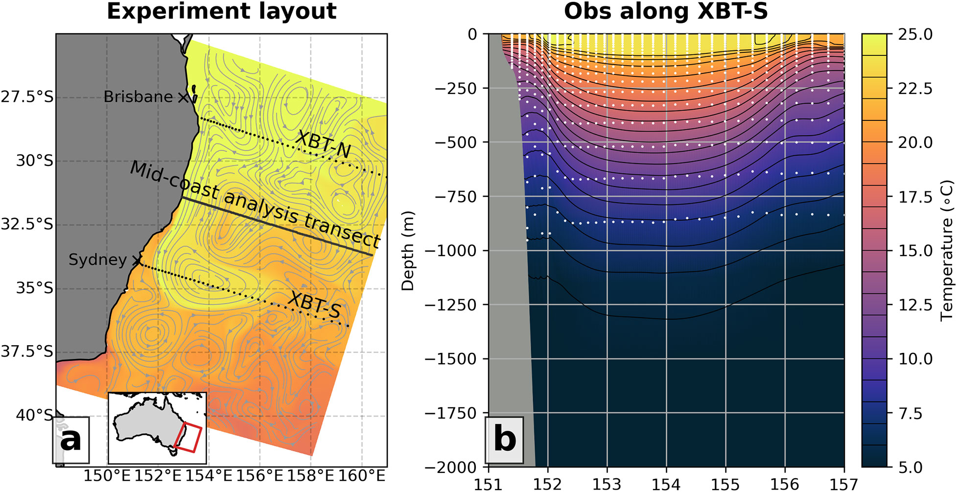
Figure 1 (A) A snapshot of model SST at 11-March 2012 is shown for the East coast of Australia. Dots mark deployment locations of XBTs along the XBT-N (beginning at ~28.5°S) and XBT-S (beginning at ~34°S) transects and the line shows the analysis transect beginning at ~31°S. Major east coast cites Brisbane and Sydney are marked, and grey vectors show model surface currents at the same time. (B) Temperature measurement locations are marked as grey dots in this vertical slice of temperature (at the same time as in panel A) along the XBT-S deployment line (see A). Inset in (A) shows model domain.

We use two model configurations: a free-running and a data assimilating configuration. The free-running model uses lateral boundary forcing (currents, temperature and salinity conditions) from BRAN2020 (Chamberlain et al., 2021) and surface forcing conditions from the Bureau of Meteorology Atmospheric high-resolution Regional Reanalysis for Australia (BARRA-R; Su et al., 2019). More details are given in Gwyther et al. (2022) and Gwyther et al. (2023).

The data assimilating configuration used for the OSSEs is based on the model setup developed by Kerry et al. (2016), and uses an Incremental Strong Constraint 4-Dimensional Variational scheme (IS4D-VAR; e.g. Moore et al., 2011). This scheme calculates the differences between a free-running ‘forecast’ and observations over a chosen assimilation window (5 days in our case), where model and observations have associated error fields. The data assimilation scheme then generates new initial and boundary conditions such that a new ‘analysis’ simulation running with these adjusted initial, boundary and surface forcing conditions has minimised differences (in a least-squares sense) from the observations. The cycle then increments forward, using the previous analysis as the initial conditions for the new forecast. This data assimilating configuration has also been used in previous studies (e.g. Kerry et al., 2016; Kerry et al., 2018; Kerry et al., 2020; Siripatana et al., 2020) including for OSSEs (Gwyther et al., 2022; Gwyther et al., 2023). The lateral forcing conditions are from BRAN2020, while atmospheric conditions are sourced from the Australian Bureau of Meteorology’s ACCESS reanalysis (Puri et al., 2013). Both free-running and data assimilating configurations use a bulk flux parameterisation (Fairall et al., 1996) for calculating surface fluxes. This difference in surface forcing conditions between configurations is a necessary requirement for ‘fraternal twin’-type OSSEs. As summarised by Halliwell et al. (2014), a balance must be sought between slightly different configurations (forcing conditions, mixing parameters or parameterisations) that introduce error and realistically test the data assimilation system, and a long-term bias that the assimilation cannot correct for. An analysis of long-term mean bias resulting from the different forcing conditions showed that bias is minimal and constrained to the surface ocean, where it can be readily corrected by assimilating SST (see Gwyther et al., 2023).

We use the free-running configuration as the reference state (referred to as the ‘ref state’), to which a series of data-assimilating simulations (the OSSEs) are compared. Values are extracted from the ref state and a representative level of error is added as a normally distributed perturbation with standard deviation equal to the observation error. The observation error is set at 0.04 m for SSH, 0.5°C for SST, and with a depth-dependent profile for XBT observations, ranging from 0.6°C to 0.12°C (more information is given in Gwyther et al., 2022). These values are then taken as the synthetic observations, and are assimilated into a perturbed data-assimilating simulation (the OSSE). Following the procedure of (Gwyther et al., 2022), we generate a perturbed simulation by initialising the free-running simulation with an 8-day offset. This perturbation is enough to cause a free-running simulation to diverge significantly from the ref state, and is thusan effective test of the performance of the data assimilation system in assimilating observations into a realistically-diverged background state. Several different perturbations were tested, including a 1-day offset, 1-month, 1-year and a climatological state, but all were found to eventually generate similarly high levels of error (not shown). We thus chose a 8-day offset as it relatively quickly diverged, but it still had mesoscale features in the approximately correct locations, which is analogous to initialisation error in a true data assimilation system. For a more detailed description of the OSSE method, Gwyther et al. (2022) gives further information and includes a schematic of the procedure (their Figure 2).

Previous work has showed that the free-running model produces accurate seasonal and interannual representations of the EAC, including the eddy field, the separation latitude, eddy kinetic energy and volume transport (e.g. Kerry et al., 2016; Kerry and Roughan, 2020; Li et al., 2021). This demonstrates that the free-running ref state is representative of the true ocean. Hence, by analogy, the impact of assimilating the synthetic observations should translate to the true ocean.

This study assesses the performance of four different hypothetical XBT observing strategies through OSSEs, by comparing these against the ref state. All OSSEs assimilate the same synthetic surface observations representing SST and SSH by extracting observations from the ref state simulation with the appropriate location and timing, as per Gwyther et al. (2022; 2023). Synthetic SSH observations are based on the spatial and temporal coverage of the global ocean along-track multi-mission sea level altimeter data. Synthetic SST observations are based on the spatial and temporal coverage of the near-real time Himawari-8 satellite product. Each OSSE also assimilates subsurface XBT-like temperature observations, also extracted from the ref state,along two transects: at ~28.5°S and ~34°S, with a horizontal observation spacing of ~12.5 km at the continental shelf break. However for each experiment the temporal repeat time of the XBT transects is different, ranging from weekly (the ‘W-12.5’ OSSE), fortnightly (the ‘2W-12.5’ OSSE), monthly (the ‘M-12.5’ OSSE) to quarterly (the ‘Q-12.5’ OSSE). Experiment names, and temporal and spatial resolutions are shown in Table 1.

TABLE 1

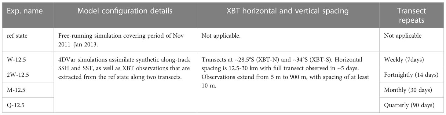
Table 1 The configurations of the free-running ref state and the four experiments are described, including the XBT horizontal and vertical spacing and XBT transect repeat time.

Subsurface observations consist of vertical temperature profiles down to 900 m, with 10 m vertical resolution (or one observation per model layer for model vertical layer spacing greater than 10 m). These observations are taken along two transects, one in the north (referred to as XBT-N; ~28.5°S) and one in the south (referred to as XBT-S; ~34°S) of the domain. The two XBT lines are chosen to represent the approximate location and vertical sampling rates of the PX30 and PX34 lines (Figure 1A shows transect locations and Figure 1B shows vertical distribution of observations along XBT-S). For ease of implementation, in our experiments, the XBT lines are oriented along grid coordinates (i.e. normal to the shore), whereas in reality the PX30 and PX34 XBT lines are along shipping routes from Brisbane to Nouméa, New Caledonia and Sydney to Wellington, New Zealand and thus at an angle to our model grid. The unique niche of the XBT dataset is the relatively fine spacing (10–100 km) between vertical profiles along defined repeat transects, allowing the resolution of a broad spectrum of processes, from eddies to basin-scale circulation (Smith et al., 1999).

All OSSEs assimilate surface observations (SSH and SST; see above) and subsurface temperature observations along both the northern transect and the southern transects, with horizontal XBT spacing of 12.5 km to 30 km (every 5 model cells) and 5-days to sample the transects. Each OSSE has different XBT transect repeat times: The W-12.5 OSSE has a transect repeat every week, the 2W-12.5 OSSE has transect repeats every two weeks, the M-12.5 has transect repeats every month (30 days) and the Q-12.5 has transect repeats every quarter year (90 days). The Q-12.5 OSSE represents the true Scripps XBT lines most closely in spatial resolution and temporal repeat time. The other OSSEs (W-12.5, 2W-12.5 and M-12.5) represent how a higher-frequency sampling scheme will impact simulated representation of the ocean.

3 Results

3.1 Modes of variability in the surface and subsurface EAC

We firstly use the ref state to explore the important spatial and temporal modes of variability of the EAC over the one-year simulation. The goal of this is to gain an understanding of the key frequencies and scales of variability, so that we can better interpret the effectiveness of observing strategies with different sampling times and lengths.

The time evolution of several surface and subsurface quantities in the ref state simulation at ~34°S are shown in Figure 2. The surface fields clearly display the seasonal cycle (transition of high to low SST anomaly from 2012-02 to 2012-08; Figure 2A) and the passage of anticyclonic and cyclonic eddies towards the south-west (anticyclonic at 2012-03 and cyclonic at 2012-11; Figure 2B). The subsurface fields at 500 m are less influenced by seasonal processes, instead being dominated by the passage of eddies (Kerry et al., 2018), and are below the EAC core depth (Gwyther et al., 2022). The most noticeable feature in the Hovmöller diagram of temperatureat 500 m is the temperature increases associated with the passing of warm core, anticyclonic eddies (and vice versa for some cyclonic eddies, e.g. mid-August 2012; Figure 2C). Eddy kinetic energy (EKE; defined as the squared anomaly in velocities from the 2012–2013 mean) at 500 m increases as the largest eddies cross the transect (Figure 2D). The consistent slopes of EKE features in the Hovmöller diagram capture the south-westwards trajectory of the largest (i.e. high EKE) eddies in this region.

FIGURE 2

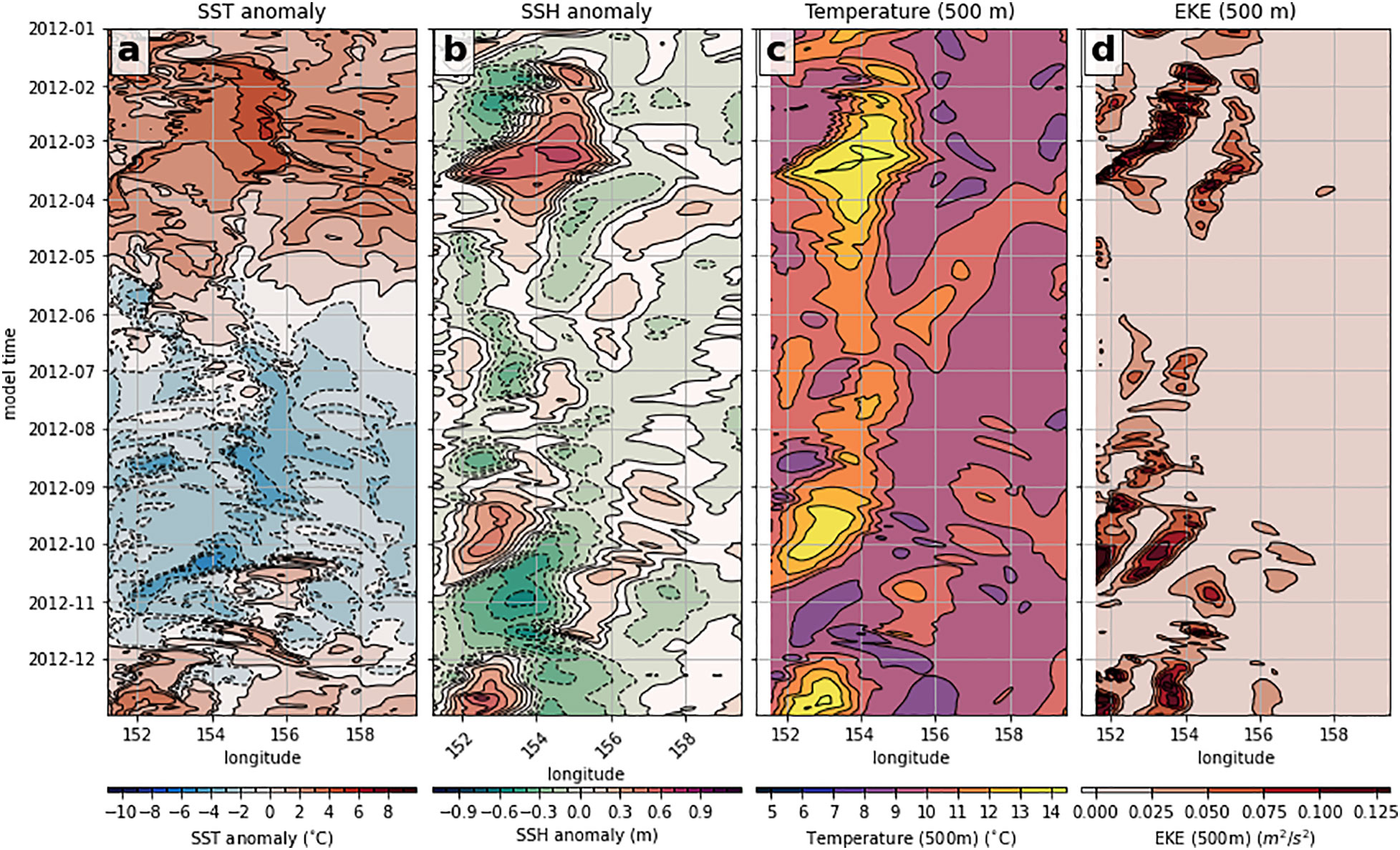
Figure 2 Hovmöller diagrams show the longitude–time variability in the ref state along the XBT-S transect (see Figure 1) for two surface quantities (A) SST anomaly, (B) SSH anomaly, and two subsurface quantities (C) temperature at 500 m and (D) EKE at 500 m. All anomalies are calculated by subtracting the mean value at each longitude over the time period Jan-2012–Jan-2013. Contour intervals are indicated with marks in the colourbar.

The variability in the EKE at 500 m can be explored further with a frequency-wavenumber spectrum analysis (Figure 3A). The spectrum is calculated by taking the 2-dimensional fourier transform of a longitude-time field, which in our case is the EKE anomaly at 500 m (Figure 2A) and the x and y axes are scaled to show periodicity and wavelength. The log₁₀ wavelength-period power spectrum shows several features: higher power at long wavelengths and monthly–seasonal timescales; and, a distinct band of increased power that runs from approximately fortnightly–monthly and very long wavelengths, through decreasing period and wavelengths to approximately daily periods and 30–40 km wavelengths. This band of increased variability is likely associated with the Rossby-mesoscale-submesoscale energy pathway and dynamics, as identified by, for example, by Torres et al. (2018). On either side of this feature (short wavelength and long period, or long wavelength and short period) there is comparatively low power. The two diagonal grey lines in Figure 3A represent a non-dispersive relationship, ω=ck, for different values of the phase speed c. These represent the frequency-wavenumber relationships for mesoscale anomalies propagating with phase speeds of c = 8 km/day and 20 km/day. The bracketing of the high-power band by these relationships further confirms that the source of this band of power is mesoscale interactions.

FIGURE 3

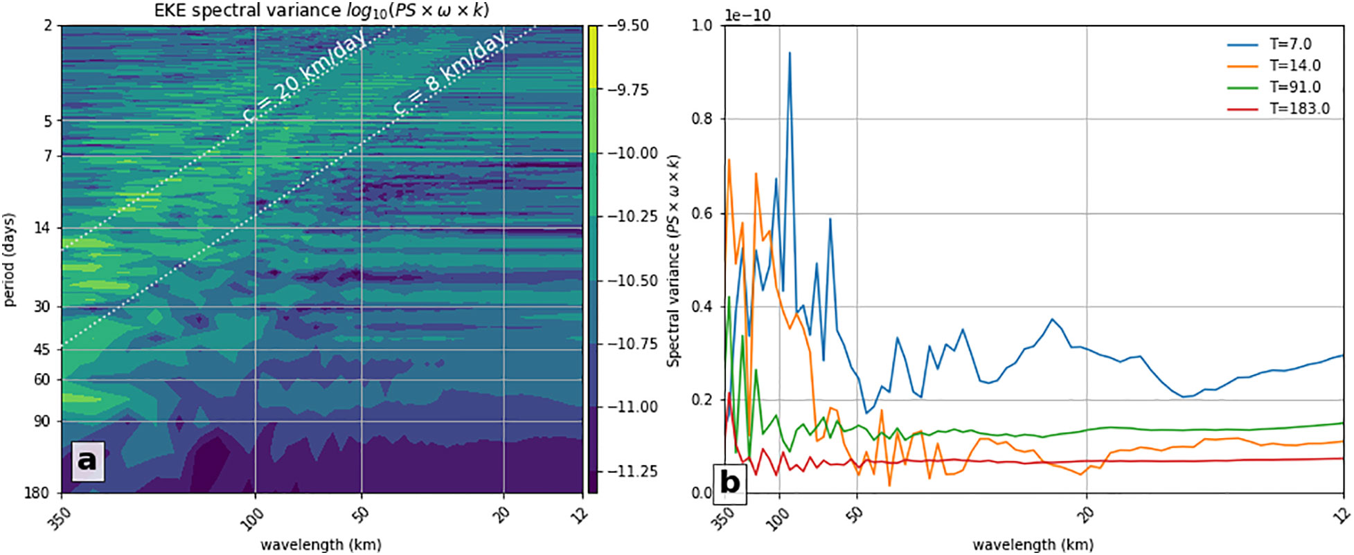
Figure 3 The variability of the EKE anomaly at 500 m along the XBT-S transect is explored for the ref state over the period Jan 2012–Jan 2013, with the (A) log₁₀ wavelength–period power spectrum of the EKE at 500 m and (B) power spectrum of the EKE at 500 m at four selected periodicities. In both panels, the power spectrum is the variance-preserving spectral density, calculated as the power scaled by the frequency and wavenumber, which more evenly weights signalsat higher frequencies and smaller length-scales. The chosen periodicities in (B) are 7 days, 14 days, ~90 days and ~180 days. The EKE anomaly is calculated by subtracting the EKE from the time-mean EKE at each longitude. The grey dashed lines in (A) show the non-dispersive relationship, ω=ck, between frequency ω and wavenumber k. The slope of the line, c, corresponds to the eddy phase speed, which is shown for two values: 8 km/day and 20 km/day.

The frequency-wavenumber power spectrum can be further analysed at several important periods, as shown in Figure 3B). Here, we show the spectral variance which we calculate by scaling the power spectrum by the frequency and wavenumber, leading to a more even weighting of signals across all frequencies and wavenumbers. The power contained at each chosen time-scale is shown to decrease with increasing period (e.g. compare 7 days to 90 days; Figure 3B). This shows that sampling at lower frequencies will truncate a significant portion of the EKE variability spectrum, and could alias high-frequency EKE energy into lower frequency modes.

Singular spectrum analysis (SSA; see Elsner and Tsonis, 1996) is used to decompose the linearly detrended time series of EKE at 500 m in the ref state at each spatial location. Different time bands are chosen to perform SSA and the variance explained by the reconstructed components are plotted for each spatial location. Benefits of SSA include that it is data-driven and works only in the time-dimension. As a result, it is less affected by the choice of basis vectors and boundary effects (e.g. EOF analyses). The percentage of total variance in EKE at 500 m that is captured over four chosen time bands are shown in Figure 4. The percentage of variance explained by processes with weekly or greater periodicity is high (spatial mean explained variance is 88%; Figure 4A), which shows that in this simulation almost all variability in the EKE field is occurring with a weekly or longer period. For fortnightly and monthly periods or longer, the percentageof explained variance drops to spatial mean values of 73% and 49%, respectively (Figures 4B, C). For quarterly periods or longer, the percentage of variance captured in that time range is small, 19% on average over the model domain (Figure 4D). Together, this illustrates that the proportion of the ocean variability that is captured by subsurface sampling will decrease with decreasing sampling frequency.

FIGURE 4

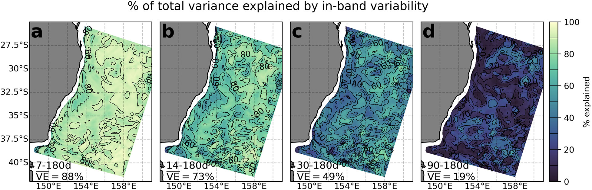
Figure 4 Singular spectrum analysis is used to quantify the percentage of the total variance in EKE at 500 m explained in four selected time bands. The variance with a period greater than (A) 7 days, (B) 14 days, (C) 30 days and (D) 90 days, and less than 180 days, is expressed as a fraction of the total variance. A high value indicates that a large amount of the full spectrum of variability at that location has a period within the indicated time band. Annotations in each plot show the band over which variance is being explained, and the spatial mean of the in-band variance explained. The contour interval is 10%.

3.2 Mean conditions under more frequent sampling

Given that EKE appears to vary more in its frequency spectrum rather than wavenumber spectrum (Figure 3), and the increasing percentage of total variance explained over longer sampling windows, there is justification for a suite of OSSEs that test the impact on EAC and eddy representation from different XBT repeat frequencies. We can assess the improvement in mean ocean conditions by comparing OSSEs with different XBT repeat frequency to the ref state.

The transect mean RMS error in temperature along three representative transects (the XBT-N, mid-coast and XBT-S lines; see Figure 1 for locations) show the improvement in representation with more frequent sampling (Figure 5). For all transects shown, the improvement in temperature RMS by increasing from quarterly to monthly sampling is minimal (Figures 5A–C). In contrast, increasing sampling to weekly decreases RMS, especially in the more dynamic region south of the separation zone (Figure 5C). However, there is not consistent improvement in time series of RMS for the most rapid sampling scheme.

FIGURE 5

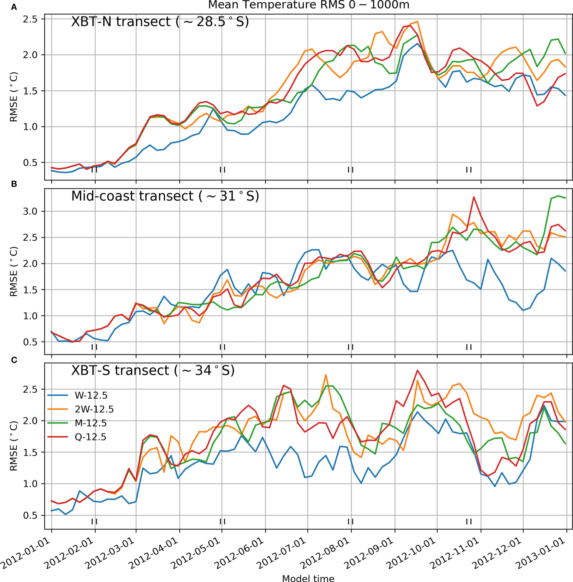
Figure 5 The transect-mean RMS error in temperature for (A) the XBT-N transect at ~28.5°S, (B) the mid-coast analysis transect at ~31°S and (C) the XBT-S transect at ~34°S for the four different OSSEs. RMS error compares the spatial-mean difference in temperature between each OSSE and the ref state. Black ticks indicate timings of quarterly XBT data assimilated into the Q-12.5 OSSE.

The vertical structure of temperature RMS, along the transects, shows an improvement when increasing the XBT repeat frequency (Figure 6). This improvement occurs both in the top 1000 m, where there are observations, and across the full water column. For example, at ~34°S, the RMS error decreases from 1.0°C to 0.94°C when increasing sampling from quarterly to monthly (see Figures 6L, K), which is otherwise not highlighted in the spatial mean RMS (Figure 5). However, there is greater improvement in RMS when increasing from monthly to weekly sampling, for example, decreasing RMS in the top 1000 m (where RMS error is highest) from 1.84°C to 1.63°C (cf. Figures E, G) at 31°S, and a larger improvement again at 34°S from 2-weekly to weekly Figures 6I, J.

FIGURE 6

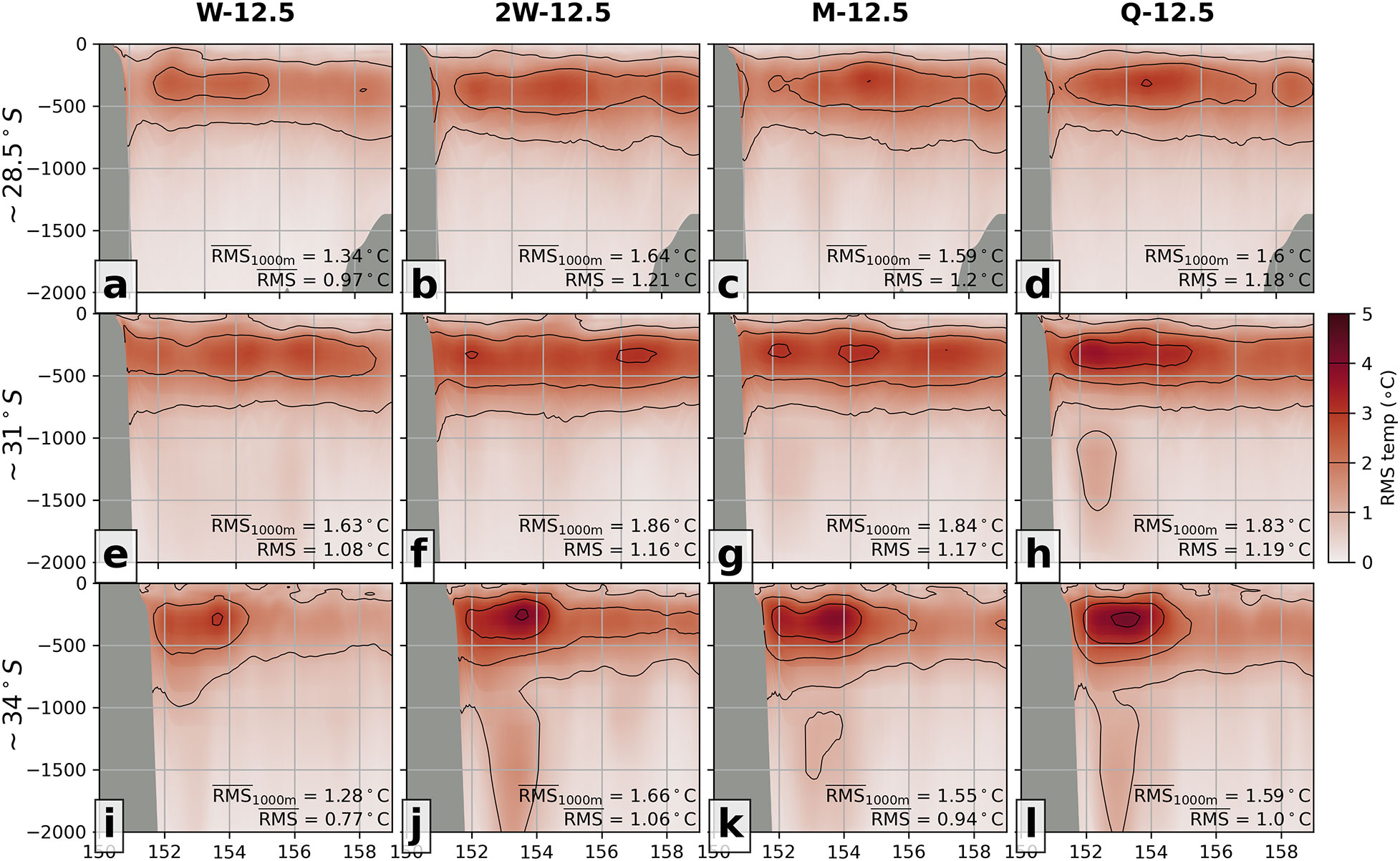
Figure 6 The RMS error in temperature, calculated for the time-mean, at the (A–D) XBT-N transect, (E–H) the mid-coast analysis transect, and (I–L) XBT-S transect, for the four different OSSEs: (A, E, I) Weekly 12.5 km, (B, F, J) Two-weekly 12.5 km, (C, G, K) Monthly 12.5 km and (D, H, L) Quarterly 12.5. RMS error is relative to the ref state, and mean values are shown in each panel for full-depth and the top 1000 m. The contour interval of 1°C is indicated with marks in the colourbar.

The spatial structure of temperature RMS clearly shows how the error is decreased by increasing XBT repeat times (Figure 7), particularly in the eddy region (indicated by the blue box, in Figure 7A). At 250 m, error is highest in the eddy region (~152°E, 36°S) but decreases as the repeat time is decreased, from a mean value of 3.1°C to 2.4°C for the eddy region (Figures 7A–D). The pattern is similar at 500 m with the W-12.5 OSSE having the lowest RMS compared to the M-12.5 and Q-12.5 OSSEs (cf. Figures 7E, G–H). At 1000 m, RMS is relatively low for all OSSEs, which reflects the lower natural variability at this depth (Figures 7I–L).

FIGURE 7

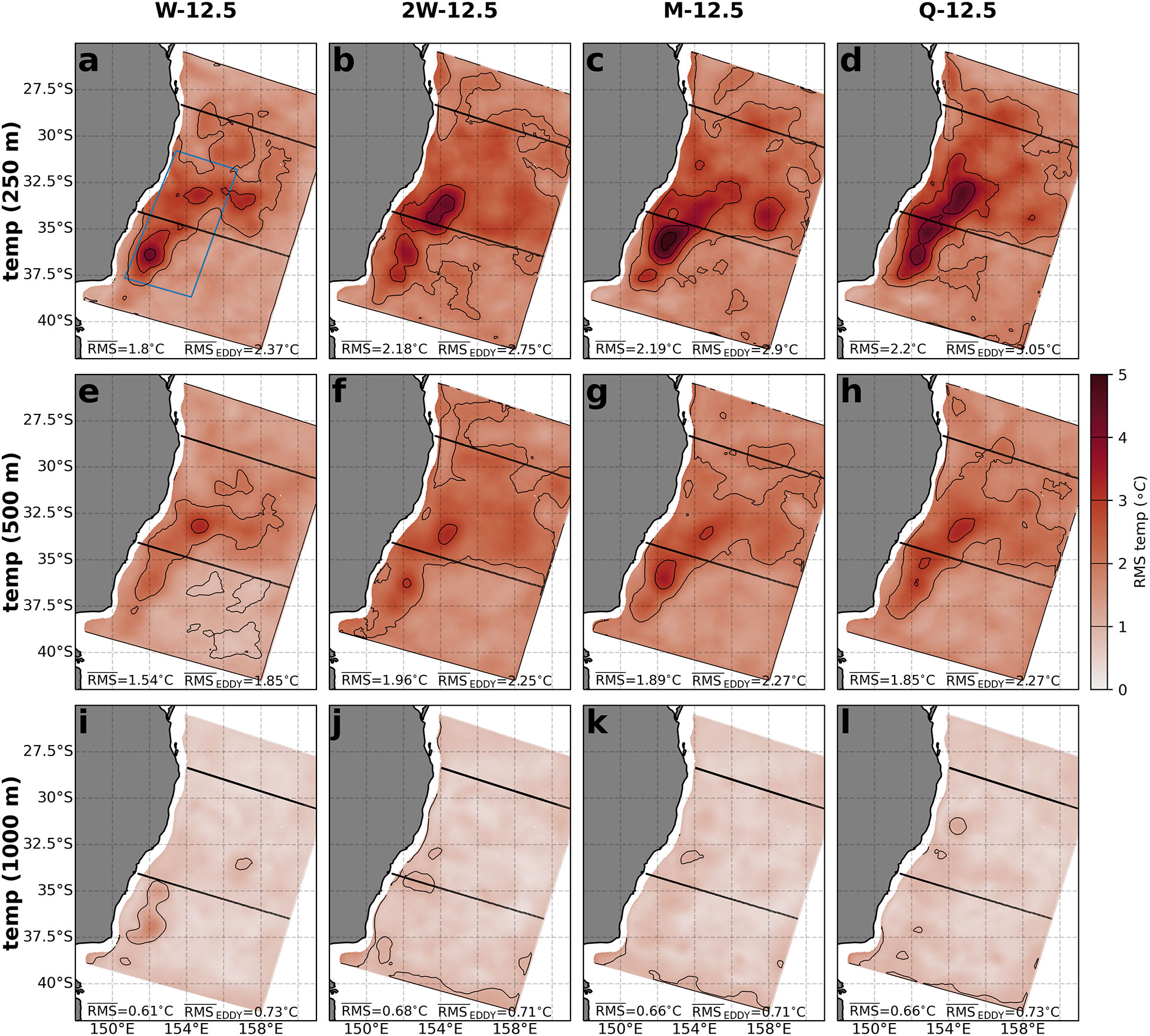
Figure 7 The RMS error in temperature, calculated for the time-mean, at depths of (A–D) 250 m, (E–H) 500 m, and (I–L) 1000 m, for the four different OSSEs: (A, E, I) Weekly 12.5 km, (B, F, J) Two-weekly 12.5 km, (C, G, K) Monthly 12.5 km and (D, H, L) Quarterly 12.5 km. RMS error is relative to the ref state, and mean values are shown in each panel for the full domain and the eddy-rich region designated by the blue box in panel (A). The contour interval of 1°C is indicated with marks in the colourbar.

Representation of the surface and subsurface salinity show no improvement with more frequent XBT observation repeats (Figure S1). This suggests that assimilation of SSH, SST and subsurface temperature is not enough to improve representation of subsurface salinity, despite any covariance of salinity and temperature properties. In our 4DVar configuration, we estimate the background error covariance matrix by factorisation (Weaver and Courtier, 2001) and prescribe univariate covariance. Covariances are assumed to be static with isotropic horizontal and vertical length scales, with flow-dependence being introduced by updating the tangent-linear and adjoint models with the time evolution of the background. Consequently, salinity is not set to covary with temperature, which may contribute to explaining this result. Compare this to Balmaseda et al. (2013), who show improvement in salinity through assimilation of temperature observations via the balance operators.

3.3 Partitioning the source of error

The RMS error in each OSSE field is the combined effect of error introduced from the data assimilation system and the error resulting from dynamic features. A bias is calculated as the time-mean OSSE field minus the time-mean — this represents the systemic error introduced through data assimilation. This bias is then subtracted from the OSSE field, and a bias-corrected RMS error is calculated — this error field now represents the differences in representation resulting from representation of dynamic ocean features.

The bias in each OSSE, calculated as the time mean of the OSSE field minus the time mean of the same field in the ref state, shows the time-averaged difference between the OSSE and the ref state (Figure 8). The bias in the SST is close to zero for all different XBT repeat times (Figures 8A–D). However, there is a cold bias at 250 m of between -1.4°C to -1.8°C for the whole domain, which is 10—13% of the mean temperature at 250 m (Figures 8E–H). At 500 m (Figures 8I–L), this bias is smaller, between -1.2°C to -1.6°C – though relative to the mean temperature at 500 m it is 13—17%; higher than at 250 m). By 1000 m, this has switched to a warm bias, particularly in the eddy region (Figures 8M–P). In almost all OSSEs, particularly in the eddy region (blue box; Figure 8A), the bias is reduced by more frequent repeat times for XBT observations (cf. -1.8°C and -2.5°C; Figures 8E, H).

FIGURE 8

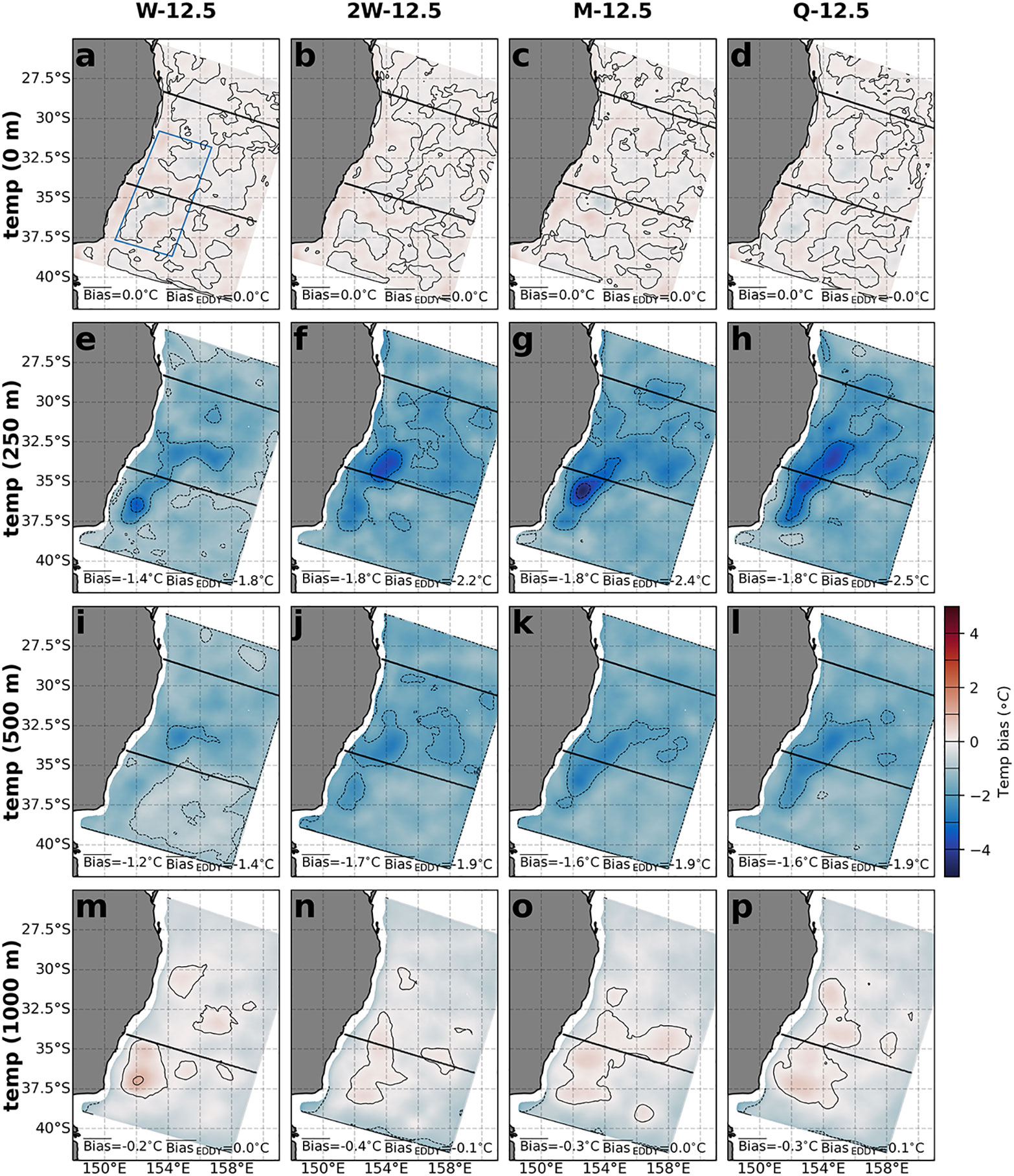
Figure 8 The bias in temperature at depths of (A–D) 0 m, (E–H) 250 m, (I–L) 500 m and (M–P) 1000 m, (E–H) 250 m, (I–L) 500 m and (M–P) 1000 m, for the four different OSSEs: (A, E, I, M) Weekly 12.5 km, (B, F, J, N) Two-weekly 12.5 km, (C, G, K, O) Monthly 12.5 km and (D, H, L, P) Quarterly 12.5 km. Bias is calculated as the time-mean difference between the OSSE and the ref state temperature fields. A positive value indicates the OSSE is warmer than the ref state, and vice versa. The mean values are shown in each panel for the full domain and the eddy-rich region designated by the blue box in panel (A). The contour interval of 1°C is indicated with marks in the colourbar.

The bias represents the time-mean difference in conditions, which we hypothesise is imposed by the data assimilation process. It causes some oceanic features to be too cold in the subsurface–500 m range, and to be too warm at depth. As a result, subtracting this bias from OSSE temperature fields before calculating the bias-corrected RMS will give the error resulting from improper representation of the dynamics. The change in this bias-corrected RMS between the different OSSEs more clearly represents how increasingly frequent XBT repeat times better capture ocean dynamics. The bias-corrected RMS in temperature fields for each OSSE are shown in Figure 9. There is a consistent improvement in bias-corrected error at 250 m for the whole domain and for the eddy region as XBT repeat frequency is increased (Figures 9A–D). At least fortnightly XBT observations are required to reduce RMS in the eddy region below 30°S. The improvement at 500 m and 1000 m is again greatest for weekly sampling (Figures 9E, I), though the improvement over fortnightly and slower sampling is minimal.

FIGURE 9

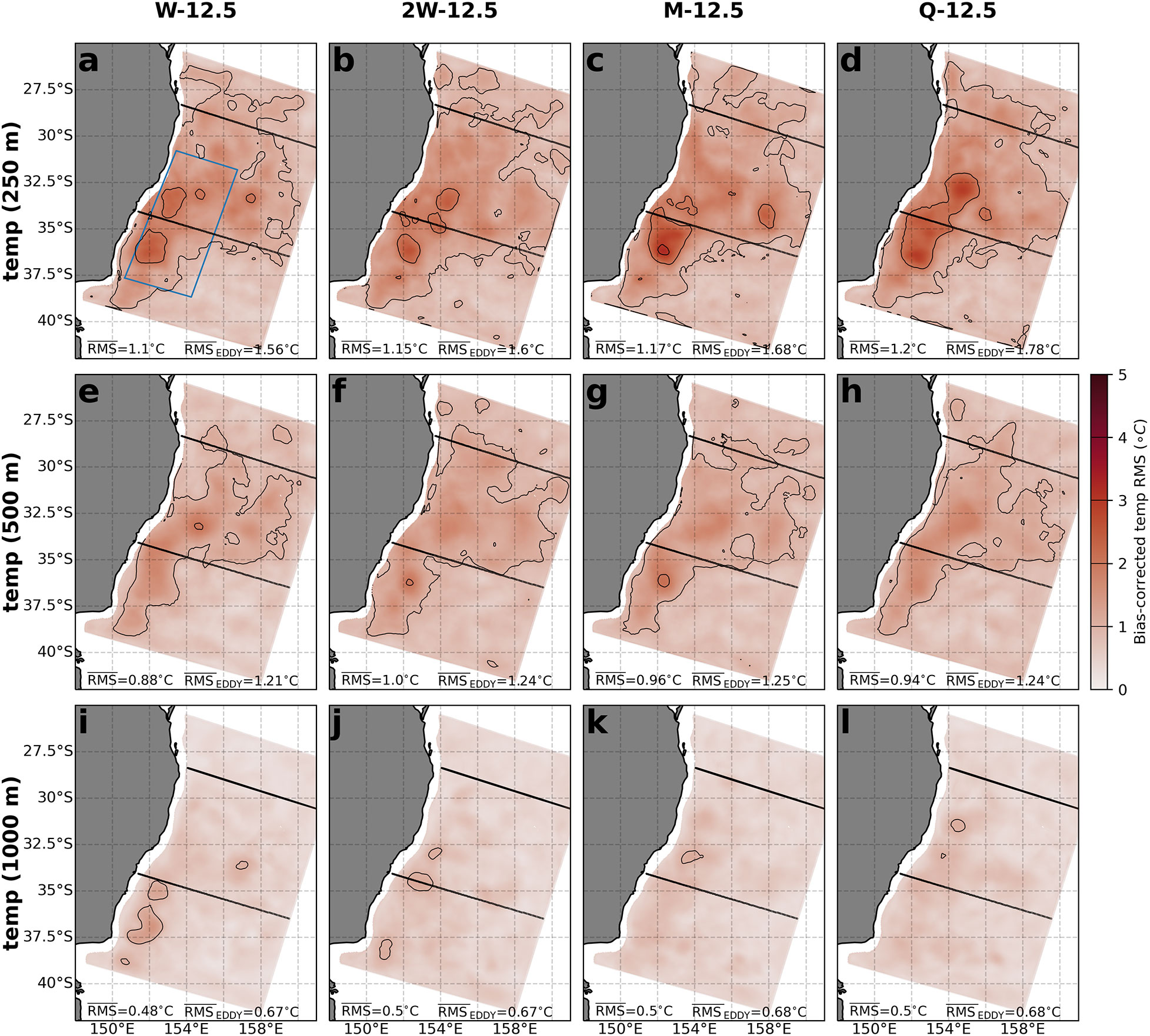
Figure 9 The bias-corrected RMS in temperature at depths of (A–D) 250 m, (E–H) 500 m, (I–L) 1000 m, for the four different OSSEs: (A, E, I) Weekly 12.5 km, (B, F, J) Two-weekly 12.5 km, (C, G, K) Monthly 12.5 km and (D, H, L) Quarterly 12.5 km.

4 Discussion

There are different modes of variability present in the ocean, from fast (e.g. tidal) to slow (e.g. climate modes) timescales and from small (e.g. eddy cascade) to large (e.g. gyre circulation) spatial scales. When designing an observation strategy, a choice must be made as to what portion of this period-wavelength phase spectrum should be sampled. Processes that are outside of the sampled portion of the spectrum are not measured enough (in time or space) to discern the process and may be aliased into thesampled portion of the spectrum. These processes either require more rapid or finer spaced sampling (i.e. for discerning small or fast scale processes), or, longer or broader sampling (i.e. for capturing large scale or slow processes). Likewise, model resolution must be fine enough that any small scale processes that are observed can actually be resolved by the model simulation – though there could be inherent limits to predictability at very fine, submesoscale resolutions (Sandery and Sakov, 2017).

We have shown that in the EAC (using our ref state simulation), ocean surface processes display a wide variety of scales, from weekly changes to seasonal variability in SST (Figure 2A). In the subsurface ocean at 500 m, the most obvious processes are eddy dynamics, which have small scale and fast changes in temperature and EKE (Figures 2C, D). Indeed, inspection of the variability period-wavelength spectrum of EKE at 500 m shows two key features: higher power at the large scales (>100 km and 30–180 days), and a band of increased power stretching from ~350 km/monthly to 30-40 km/daily wavelengths and periods, which likely represents the increased variability associated with the Rossby-mesoscale-submesoscale energy pathway (Figure 3A). Sampling any less frequently than monthly will truncate a large portion of this mesoscale energy pathway. Given that we can quantify the amount of variability with different spatial scales, we can directly describe the portion of the total variability that is captured by repeat sampling at chosen frequencies. In particular, for EKE at 500 m, quarterly sampling captures ~20% of total variability, while increasing to monthly sampling captures ~50%. More rapid sampling rates at fortnightly and weekly frequencies captures ~70% and ~90% of the total EKE variability (Figure 4). Note that since data assimilation systems will not exactly match observations (for e.g. due to observation error), we would only expect these patterns to be approached in the long-term.

While there is no obvious reduction in transect-mean error when sampling is increased from quarterly to fortnightly, reduced RMS is noticeable with weekly sampling (Figures 5A–C). This shows that infrequent observations (i.e. quarterly through to fortnightly subsurface observation repeats) have limited impact on constraining mean subsurface conditions, and highlights the importance of regularly assimilating subsurface observations to maintain an accurate estimate.

This is further confirmed in the vertical transects of temperature RMS, where the highest error region (~250 m) is represented with similar error in quarterly, monthly and fortnightly sampling, but is improved with weekly sampling (cf. Figures 6A–D). Horizontal fields of temperature RMS show that the greatest improvement in representation is indeed in the 250 m depth range, and particularly in the high eddy energy region. This confirms that repeat sampling of at least weekly frequency is required to improve the mean representation of heat in the critical 250 m depth range in the northern upstream region (Figure 7A), separation region (Figure 7E) and southern high eddy region (Figure 7I). Indeed, this confirms the importance of higher repeat frequency observations as suggested by the variability analysis, where sampling at fortnightly–weekly frequencies is required to capture 60–80% of variability in the higher EKE region (Figures 4A, B).

Systemic error is introduced by the data assimilation system and can only be mitigated through improvements to the data assimilation system. This error could present as overly deep eddies (Siripatana et al., 2020), incorrect vertical distribution of temperature and heat content (Gwyther et al., 2022), or baroclinic mode structure (Gwyther et al., 2023). Endemic error results from the resolution of mesoscale processes and is improved by faster or higher resolution sampling. Maps of bias (Figure 8) suggest that the data assimilation process is producing a temperature structure that is too cold between 250–500 m and too warm at 1000 m. The location of the strongest bias suggests that eddies suffer disproportionately from this systemic error. The slight decrease in bias that is observed in the W-12.5 OSSE, particularly for the eddy region, indicates that weekly subsurface temperature observations are playing an important role in repeatedly correcting the vertical structure. The bias-corrected temperature RMS shows that the largest improvement in representation is in the 250 m depth range, which is achieved by taking XBT measurements at faster than monthly frequency. Improvement at 500 m is smaller, though, as most error is concentrated in the 250 m range, this may be acceptable. The improvement in increasing XBT sampling time from quarterly to monthly (see reduction in RMS in the separation zone; Figure 9D) may represent improvements in capturing seasonal-scale processes, such as mean separation latitude (Ypma et al., 2016; Oke et al., 2019), jet core velocity and EKE (Archer et al., 2017). The comparatively larger reduction in RMS observed when moving to fortnightly or weekly sampling likely represents better representation of mesoscale dynamics. This is supported by the frequency analysis (Section 3.1) and by the largest RMS reduction being in the eddy region (Figures 9A, B). In Figure 7, the greatest improvement in RMS error, particularly in the eddy region, is achieved by weekly sampling. In contrast, Figure 9 shows that fortnightly sampling achieves sufficient reduction of bias-corrected RMS error in the eddy region. This indicates that the gain achieved from moving from fortnightly to weekly sampling is through reduction of the bias – likely due to the presence of subsurface observations in each assimilation window.

The large temperature bias (Figure 8) likely results from the data assimilation process itself. This could result from the specification of background error covariance matrix, which controls the influence of observations in the horizontal and vertical (Bannister, 2008) and the weighting of the model forecast (Lee and Huang, 2020). Correctly specifying the background error covariance matrix is a major challenge to accurate data assimilation simulations (see review in Moore et al., 2019). Indeed, several studies have shown that 3-dimensional structure suffers in data assimilation, even with the inclusion of the limited subsurface observations (see for e.g. Zavala-Garay et al., 2012; Pilo et al., 2018; Siripatana et al., 2020; de Paula et al., 2021; Gwyther et al., 2022; Gwyther et al., 2023).

In any case, the result is that subsurface representation needs to be constrained frequently (i.e. weekly), otherwise subsurface structure drifts too far from the truth and any improvement from observations is minimal, though this result may change for different assimilation techniques. This suggests that improvements to assimilation schemes could improve representation of the subsurface structure even in the absence of observations. Furthermore, existing observations (i.e. quarterly subsurface measurements) could have more impact than they currently do, and potentially, sampling on the mesoscale timescale would be sufficient.

5 Conclusion

Operational and research-focussed data assimilation systems benefit greatly from the high spatial resolution, coverage and relatively rapid temporal repeat times of satellite-inferred sea-surface measurements. As a result, these systems can provide accurate and representative estimates of sea surface temperature and height (and hence geostrophic currents). However, subsurface conditions such as temperature and velocities (Gwyther et al., 2022), isothermal slopes and baroclinic mode structure (Gwyther et al., 2023) are not represented with the same accuracy. These simulation inaccuracies are further compounded when trying to simulate dynamically complex 3-dimensional structures such as eddies (Gwyther et al., 2023). As a result, the assimilation of subsurface observations is critical to improving representation. While some subsurface observations are routinely assimilated into operational ocean models, many of these are sampling sparsely (e.g. Argo floats), or were designed for climatological studies(e.g. the Scripps high resolution XBT program). So, there is some justification for the re-purposing of existing subsurface sampling frameworks, at potentially faster repeat times, so as to be of more use for operational models that estimate and forecastocean conditions.

Our results have showed that frequencies of variability of interest need to be considered when assimilating subsurface observations. We have explored the benefit of assimilating data from an XBT observing network designed to observe climatological-scale processes i.e. heat fluxes through ocean basins over interannual periods. Our results show that assimilating XBT data at fortnightly repeat times would give a better representation of higher frequency processes such as mesoscale eddies. However, we also show that systemic errors in the data assimilation process itself limit the ability to represent accurate vertical structure. Improvements to the assimilation scheme to reduce systemic error and biases would therefore increase the positive benefit obtained from current and future subsurface observation systems.

Data availability statement

The raw data supporting the conclusions of this article will be made available by the authors, without undue reservation.

Author contributions

DG, MR, CK, SK conceived the study and designed and experiments. DG and CK configured the data assimilating model. DG performed the analyses. DG and MR wrote the first draft of the manuscript. All authors contributed to the manuscript editing and revisions. All authors contributed to the article and approved the submitted version.

Funding

This research and DG were partially supported by Australian Research Council Industry Linkage Grant LP170100498 to MR, SK, and CK.

Acknowledgments

Former model development was supported by Australian Research Council grants DP140102337 and LP160100162 to MR. This research was undertaken with the assistance of resources and services from the National Computational Infrastructure (NCI), under the grant fu5, and computations using the computational cluster Katana (https://doi.org/10.26190/669x-a286), supported by Research Technology Services at UNSW Sydney.

Conflict of interest

The authors declare that the research was conducted in the absence of any commercial or financial relationships that could be construed as a potential conflict of interest.

Publisher’s note

All claims expressed in this article are solely those of the authors and do not necessarily represent those of their affiliated organizations, or those of the publisher, the editors and the reviewers. Any product that may be evaluated in this article, or claim that may be made by its manufacturer, is not guaranteed or endorsed by the publisher.

Supplementary material

The Supplementary Material for this article can be found online at: https://www.frontiersin.org/articles/10.3389/fmars.2022.1084784/full#supplementary-material

References

Abernathey R., Haller G. (2018). Transport by lagrangian vortices in the eastern pacific. J. Phys. Oceanography 48, 667–685. doi: 10.1175/jpo-d-17-0102.1

CrossRef Full Text | Google Scholar

Archer M. R., Roughan M., Keating S. R., Schaeffer A. (2017). On the variability of the East Australian current: Jet structure, meandering, and influence on shelf circulation. J. Geophysical Research: Oceans 122, 8464–8481. doi: 10.1002/2017jc013097

CrossRef Full Text | Google Scholar

Balmaseda M. A., Mogensen K., Weaver A. T. (2013). Evaluation of the ECMWF ocean reanalysis system ORAS4. Q. J. R. Meteorological Soc. 139, 1132–1161. doi: 10.1002/qj.2063

CrossRef Full Text | Google Scholar

Bannister R. N. (2008). A review of forecast error covariance statistics in atmospheric variational data assimilation. I: Characteristics and measurements of forecast error covariances. Q. J. R. Meteorological Soc. 134, 1951–1970. doi: 10.1002/qj.339

CrossRef Full Text | Google Scholar

Brassington G., Pugh T., Spillman C., Schulz E., Beggs H., Schiller A., et al. (2007). BLUElink> development of operational oceanography and servicing in Australia. J. Res. Pract. Inf. Technol. 39(2):151–164.

Google Scholar

Brieva D., Ribbe J., Lemckert C. (2015). Is the East Australian current causing a marine ecological hot-spot and an important fisheries near Fraser island, Australia? Estuarine Coast. Shelf Sci. 153, 121–134. doi: 10.1016/j.ecss.2014.12.012

CrossRef Full Text | Google Scholar

Carton J. A., Chepurin G., Cao X., Giese B. (2000). A simple ocean data assimilation analysis of the global upper ocean 1950–95. part I: Methodology. J. Phys. Oceanography 30, 294–309. doi: 10.1175/1520-0485(2000)030<0294:asodaa>2.0.co;2

CrossRef Full Text | Google Scholar

Chamberlain M. A., Oke P. R., Fiedler R. A. S., Beggs H. M., Brassington G. B., Divakaran P. (2021). Next generation of bluelink ocean reanalysis with multiscale data assimilation: BRAN2020. Earth System Sci. Data 13, 5663–5688. doi: 10.5194/essd-13-5663-2021

CrossRef Full Text | Google Scholar

de Paula T. P., Lima J. A. M., Tanajura C. A. S., Andrioni M., Martins R. P., Arruda W. Z. (2021). The impact of ocean data assimilation on the simulation of mesoscale eddies at são paulo plateau (Brazil) using the regional ocean modeling system. Ocean Model. 167, 101889. doi: 10.1016/j.ocemod.2021.101889

CrossRef Full Text | Google Scholar

Elsner J. B., Tsonis A. A. (1996). Singular spectrum analysis: a new tool in time series analysis (New York: Springer Science & Business Media). doi: 10.1007/978-1-4757-2514-8

CrossRef Full Text | Google Scholar

Everett J. D., Baird M. E., Oke P. R., Suthers I. M. (2012). An avenue of eddies: Quantifying the biophysical properties of mesoscale eddies in the Tasman Sea. Geophysical Research Letters 39(16). doi: 10.1029/2012GL053091

PubMed Abstract | CrossRef Full Text | Google Scholar

Fairall C. W., Bradley E. F., Rogers D. P., Edson J. B., Young G. S. (1996). Bulk parameterization of air-sea fluxes for tropical ocean-global atmosphere coupled-ocean atmosphere response experiment. J. Geophysical Research: Oceans 101, 3747–3764. doi: 10.1029/95jc03205

CrossRef Full Text | Google Scholar

Frenger I., Gruber N., Knutti R., Münnich M. (2013). Imprint of southern ocean eddies on winds, clouds and rainfall. Nat. Geosci. 6, 608–612. doi: 10.1038/ngeo1863

CrossRef Full Text | Google Scholar

Gasparin F., Guinehut S., Mao C., Mirouze I., Rémy E., King R. R., et al. (2019). Requirements for an integrated in situ Atlantic ocean observing system from coordinated observing system simulation experiments. Front. Mar. Sci. 6. doi: 10.3389/fmars.2019.00083

CrossRef Full Text | Google Scholar

Gwyther D. E., Keating S. R., Kerry C., Roughan M. (2023) How does 4DVar data assimilation affect the vertical representation of mesoscale eddies? A case study with observing system simulation experiments (OSSEs) using ROMS v3.9. Geosci. Model. Dev. 16:157–178 doi: 10.5194/gmd-16-157-2023

CrossRef Full Text | Google Scholar

Gwyther D. E., Kerry C., Roughan M., Keating S. R. (2022). Observing system simulation experiments reveal that subsurface temperature observations improve estimates of circulation and heat content in a dynamic western boundary current. Geoscientific Model. Dev. 15, 6541–6565. doi: 10.5194/gmd-15-6541-2022

CrossRef Full Text | Google Scholar

Halliwell G. R., Kourafalou V., Hénaff M. L., Shay L. K., Atlas R. (2015). OSSE impact analysis of airborne ocean surveys for improving upper-ocean dynamical and thermodynamical forecasts in the gulf of Mexico. Prog. Oceanography 130, 32–46. doi: 10.1016/j.pocean.2014.09.004

CrossRef Full Text | Google Scholar

Halliwell G. R., Srinivasan A., Kourafalou V., Yang H., Willey D., Hénaff M. L., et al. (2014). Rigorous evaluation of a fraternal twin ocean OSSE system for the open gulf of Mexico. J. Atmospheric Oceanic Technol. 31, 105–130. doi: 10.1175/jtech-d-13-00011.1

CrossRef Full Text | Google Scholar

Kerry C., Powell B., Roughan M., Oke P. (2016). Development and evaluation of a high-resolution reanalysis of the East Australian current region using the regional ocean modelling system (ROMS 3.4) and incremental strong-constraint 4-dimensional variational (IS4D-var) data assimilation. Geoscientific Model. Dev. 9, 3779–3801. doi: 10.5194/gmd-9-3779-2016

CrossRef Full Text | Google Scholar

Kerry C., Roughan M. (2020). Downstream evolution of the East Australian current system: Mean flow, seasonal, and intra-annual variability. J. Geophysical Research: Oceans 125, e2019JC015227. doi: 10.1029/2019jc015227

CrossRef Full Text | Google Scholar

Kerry C., Roughan M., Powell B. (2018). Observation impact in a regional reanalysis of the East Australian current system. J. Geophysical Research: Oceans 123, 7511–7528. doi: 10.1029/2017jc013685

CrossRef Full Text | Google Scholar

Kerry C., Roughan M., Powell B. (2020). Predicting the submesoscale circulation inshore of the East Australian current. J. Mar. Syst. 204, 103286. doi: 10.1016/j.jmarsys.2019.103286

CrossRef Full Text | Google Scholar

Klocker A., Abernathey R. (2014). Global patterns of mesoscale eddy properties and diffusivities. J. Phys. Oceanography 44, 1030–1046. doi: 10.1175/jpo-d-13-0159.1

CrossRef Full Text | Google Scholar

Lambaerts J., Lapeyre G., Plougonven R., Klein P. (2013). Atmospheric response to sea surface temperature mesoscale structures. J. Geophysical Research: Atmospheres 118, 9611–9621. doi: 10.1002/jgrd.50769

CrossRef Full Text | Google Scholar

Lee J. C. K., Huang X.-Y. (2020). Background error statistics in the tropics: Structures and impact in a convective-scale numerical weather prediction system. Q. J. R. Meteorological Soc. 146, 2154–2173. doi: 10.1002/qj.3785

CrossRef Full Text | Google Scholar

Li J., Roughan M., Kerry C. (2021). Dynamics of interannual eddy kinetic energy modulations in a Western boundary current. Geophysical Res. Lett. 48, e2021GL094115. doi: 10.1029/2021gl094115

CrossRef Full Text | Google Scholar

Li J., Roughan M., Kerry C. (2022a). Drivers of ocean warming in the western boundary currents of the southern hemisphere. Nat. Climate Change 12, 901–909. doi: 10.1038/s41558-022-01473-8

CrossRef Full Text | Google Scholar

Li J., Roughan M., Kerry C., Rao S. (2022b). Impact of mesoscale circulation on the structure of river plumes during large rainfall events inshore of the east australian current. Front. Mar. Sci. 9. doi: 10.3389/fmars.2022.815348

PubMed Abstract | CrossRef Full Text | Google Scholar

Malan N., Archer M., Roughan M., Cetina-Heredia P., Hemming M., Rocha C., et al. (2020). Eddy-driven cross-shelf transport in the East Australian current separation zone. J. Geophysical Research: Oceans 125, e2019JC015613. doi: 10.1029/2019jc015613

CrossRef Full Text | Google Scholar

Moore A. M., Arango H. G., Broquet G., Powell B. S., Weaver A. T., Zavala-Garay J. (2011). The regional ocean modeling system (ROMS) 4-dimensional variational data assimilation systems: Part I - system overview and formulation. Prog. Oceanography 91, 34–49. doi: 10.1016/j.pocean.2011.05.004

CrossRef Full Text | Google Scholar

Moore A. M., Martin M. J., Akella S., Arango H. G., Balmaseda M., Bertino L., et al. (2019). Synthesis of ocean observations using data assimilation for operational, real-time and reanalysis systems: A more complete picture of the state of the ocean. Front. Mar. Sci. 6. doi: 10.3389/fmars.2019.00090

CrossRef Full Text | Google Scholar

Moore A. M., Zavala-Garay J., Arango H. G., Edwards C. A., Anderson J., Hoar T. (2020). Regional and basin scale applications of ensemble adjustment kalman filter and 4D-var ocean data assimilation systems. Prog. Oceanography 189, 102450. doi: 10.1016/j.pocean.2020.102450

CrossRef Full Text | Google Scholar

Morris M., Roemmich D., Cornuelle B. (1996). Observations of variability in the south pacific subtropical gyre. J. Phys. Oceanography 26, 2359–2380. doi: 10.1175/1520-0485(1996)026<2359:oovits>2.0.co;2

CrossRef Full Text | Google Scholar

Oke P. R., Roughan M., Cetina-Heredia P., Pilo G. S., Ridgway K. R., Rykova T., et al. (2019). Revisiting the circulation of the East Australian current: Its path, separation, and eddy field. Prog. Oceanography 176, 102139. doi: 10.1016/j.pocean.2019.102139

CrossRef Full Text | Google Scholar

Oke P. R., Sakov P., Cahill M. L., Dunn J. R., Fiedler R., Griffin D. A., et al. (2013). Towards a dynamically balanced eddy-resolving ocean reanalysis: BRAN3. Ocean Model. 67, 52–70. doi: 10.1016/j.ocemod.2013.03.008

CrossRef Full Text | Google Scholar

Oliver H., Zhang W. G., Smith W. O., Alatalo P., Chappell P. D., Hirzel A. J., et al. (2021). Diatom hotspots driven by Western boundary current instability. Geophysical Res. Lett. 48, e2020GL091943. doi: 10.1029/2020gl091943

CrossRef Full Text | Google Scholar

Pilo G. S., Oke P. R., Coleman R., Rykova T., Ridgway K. (2018). Impact of data assimilation on vertical velocities in an eddy resolving ocean model. Ocean Model. 131, 71–85. doi: 10.1016/j.ocemod.2018.09.003

CrossRef Full Text | Google Scholar

Puri K., Dietachmayer G., Steinle P., Dix M., Rikus L., Logan L., et al. (2013). Implementation of the initial access numerical weather prediction system. Aust. Meteorological Oceanographic J. 63, 265–284. puri2013implementation. doi: 10.22499/2.6302.001

CrossRef Full Text | Google Scholar

Rocha C., Edwards C. A., Roughan M., Cetina-Heredia P., Kerry C. (2019). A high-resolution biogeochemical model (ROMS 3.4+bio_Fennel) of the East Australian current system. Geoscientific Model. Dev. 12, 441–456. doi: 10.5194/gmd-12-441-2019

CrossRef Full Text | Google Scholar

Roemmich D., Cornuelle B. (1990). Observing the fluctuations of gyre-scale ocean circulation: A study of the subtropical south pacific. J. Phys. Oceanography 20, 1919–1934. doi: 10.1175/1520-0485(1990)020<1919:otfogs>2.0.co;2

CrossRef Full Text | Google Scholar

Roemmich D., Gilson J., Willis J., Sutton P., Ridgway K. (2005). Closing the time-varying mass and heat budgets for large ocean areas: The tasman box. J. Climate 18, 2330–2343. doi: 10.1175/jcli3409.1

CrossRef Full Text | Google Scholar

Sandery P. A., Sakov P. (2017). Ocean forecasting of mesoscale features can deteriorate by increasing model resolution towards the submesoscale. Nat. Commun. 8:1566. doi: 10.1038/s41467-017-01595-0

CrossRef Full Text | Google Scholar

Shchepetkin A. F., McWilliams J. C. (2005). The regional oceanic modeling system (ROMS): a split-explicit, free-surface, topography-following-coordinate oceanic model. Ocean Model. 9, 347–404. doi: 10.1016/j.ocemod.2004.08.002

CrossRef Full Text | Google Scholar

Siripatana A., Kerry C., Roughan M., Souza J. M. A. C., Keating S. (2020). Assessing the impact of nontraditional ocean observations for prediction of the East Australian current. J. Geophysical Research: Oceans 125, e2020JC016580. doi: 10.1029/2020jc016580

CrossRef Full Text | Google Scholar

Smith N. R., Harrison D., Bailey R., Alves O., Delcroix T., Hanawa K., et al. (1999). The role of XBT sampling in the ocean thermal network (White paper, OceanObs99 Saint Raphaël, France).

Google Scholar

Su C.-H., Eizenberg N., Steinle P., Jakob D., Fox-Hughes P., White C. J., et al. (2019). BARRA v1.0: the bureau of meteorology atmospheric high-resolution regional reanalysis for Australia. Geoscientific Model. Dev. 12, 2049–2068. doi: 10.5194/gmd-12-2049-2019

CrossRef Full Text | Google Scholar

Torres H. S., Klein P., Menemenlis D., Qiu B., Su Z., Wang J., et al. (2018). Partitioning ocean motions into balanced motions and internal gravity waves: A modeling study in anticipation of future space missions. J. Geophysical Research: Oceans 123, 8084–8105. doi: 10.1029/2018jc014438

CrossRef Full Text | Google Scholar

Weaver A., Courtier P. (2001). Correlation modelling on the sphere using a generalized diffusion equation. Q. J. R. Meteorological Soc. 127, 1815–1846. doi: 10.1002/qj.49712757518

CrossRef Full Text | Google Scholar

Whiteway T. (2009) Australian Bathymetry and topography grid, june 2009. Available at: http://dx.doi.org/10.4225/25/53D99B6581B9A (Accessed 08-02-2021). Dataset.

Google Scholar

Wijffels S., Roemmich D., Monselesan D., Church J., Gilson J. (2016). Ocean temperatures chronicle the ongoing warming of earth. Nat. Climate Change 6, 116–118. doi: 10.1038/nclimate2924

CrossRef Full Text | Google Scholar

Wong A. P. S., Wijffels S. E., Riser S. C., Pouliquen S., Hosoda S., Roemmich D., et al. (2020). Argo data 1999–2019: Two million temperature-salinity profiles and subsurface velocity observations from a global array of profiling floats. Front. Mar. Sci. 7. doi: 10.3389/fmars.2020.00700

CrossRef Full Text | Google Scholar

Young J., Hobday A., Campbell R., Kloser R., Bonham P., Clementson L., et al. (2011). The biological oceanography of the East Australian current and surrounding waters in relation to tuna and billfish catches off eastern Australia. Deep Sea Res. Part II: Topical Stud. Oceanography 58, 720–733. doi: 10.1016/j.dsr2.2010.10.005

CrossRef Full Text | Google Scholar

Ypma S. L., van Sebille E., Kiss A. E., Spence P. (2016). The separation of the East Australian current: A Lagrangian approach to potential vorticity and upstream control. J. Geophysical Research: Oceans 121, 758–774. doi: 10.1002/2015jc011133

CrossRef Full Text | Google Scholar

Zavala-Garay J., Wilkin J. L., Arango H. G. (2012). Predictability of mesoscale variability in the East Australian current given strong-constraint data assimilation. J. Phys. Oceanography 42, 1402–1420. doi: 10.1175/jpo-d-11-0168.1

CrossRef Full Text | Google Scholar