Environmental Change at Deep-Sea Sponge Habitats Over the Last Half Century: A Model Hindcast Study for the Age of Anthropogenic Climate Change

Introduction

Deep-sea sponges are found globally in a range of settings, such as fjords, continental shelf edges/slopes, mid-ocean ridges, and seamounts (Cárdenas and Rapp, 2015; Roberts et al., 2018; Kazanidis et al., 2019; Meyer et al., 2020). They also occur across a wide depth range, through the mesopelagic and bathyal zones and even at abyssal and hadal depths (Vacelet, 2007; Hestetun et al., 2019). The numerous known sponge-dominated communities spread throughout the North Atlantic Ocean include boreo-Arctic astrophorid grounds (Klitgaard and Tendal, 2004; Murillo et al., 2012; Cárdenas et al., 2013; Knudby et al., 2013; Roberts et al., 2018): multispecific assemblages of large astrophorid species and/or glass sponges (Hexactinellida), which are often further classified as either boreal (e.g., off the Faroe Islands, Norway, South of Iceland, the Labrador and Newfoundland shelves, and parts of Davis Strait) or cold-water grounds (e.g., north of Iceland, the Denmark Strait, off East Greenland, and north of Svalbard). There are also monospecific aggregations of glass sponges (Rice et al., 1990; Dohrmann et al., 2012; Beazley et al., 2021; Rodríguez-Basalo et al., 2021), such as Pheronema carpenteri (e.g., along the European and northwest African continental shelves and slopes, and off the Azores archipelago), Nodastrella asconemaoida (Rockall Bank, west of Ireland), Asconema setubalense (Le Danois Bank, Cantabrian Sea), and Vazella pourtalesi (Scotian Shelf, Canada). Beyond these ground types, there are also sponge-dominated communities of variable species diversity, composition, density and patchiness, which do not fall neatly into the above categories (e.g., sponge gardens found in the Aviles Canyon of the Cantabrian Sea, on the seamounts of the Azores archipelago, and on the New England seamounts).

Deep-sea sponges are presently the subject of much scientific interest, owing to the realization that sponges and sponge-dominated ecosystems provide a multitude of important goods and services (Hogg et al., 2010). They are known to play a key role in habitat provision (Bett and Rice, 1992; Hawkes et al., 2019), acting as ecosystem engineers and sustaining hotspots of biomass and biodiversity (Klitgaard, 1995; Beazley et al., 2013). They are also a significant biotechnological and biomedical resource: their secondary metabolites are a promising source of bioactive compounds and their structures have inspired biomimetic research (Belarbi, 2003; Sundar et al., 2003; Leal et al., 2012; Dudik et al., 2018). Sponges, and particularly dense ground aggregations, are also likely to be of fundamental importance to biogeochemical cycling, benthic-pelagic coupling, and carbon and silicon sequestration in the deep sea (Pile and Young, 2006; Bell, 2008; Bart et al., 2021).

Deep-sea sponges are known to be vulnerable to the direct and indirect effects of physical disturbance, for example from bottom trawling (Morrison et al., 2020; Wurz et al., 2021), and deep-sea sponge grounds have been classified as a “habitat under immediate threat and/or decline” by the OSPAR Commission (OSPAR Commission, 2008) and a “vulnerable marine ecosystem (VME)” by the Food and Agriculture Organization of the United Nations (FAO, 2009). Since certain deep-sea sponge species can be very slow-growing (Pusceddu et al., 2014), reproduce infrequently (Klitgaard and Tendal, 2004), and take millennia to form grounds (Murillo et al., 2016), it is often inferred that sponges may also be vulnerable to other environmental change (Hogg et al., 2010). There is concern in the deep-sea research community around changes occurring because of anthropogenic activities and potentially moving beyond the limits of past natural variability. Relatively little is known still about deep-sea sponge sensitivities to environmental fluctuations and more persistent trends under climate change (Maldonado, 2006; Bell, 2008).

Recent studies have been able to characterize present-day environmental conditions and short timescale (sub-hourly to seasonal) variability inside sponge grounds from in situ measurements (e.g., Roberts et al., 2018; Davison et al., 2019; Hanz et al., 2021a,b). Two studies, focused on different sponge grounds in the Northwest Atlantic, have demonstrated that some sponge populations may have persisted in the face of considerable past environmental variability over longer timescales (centuries to millennia) (Murillo et al., 2016; Beazley et al., 2018). Looking forward in time, Beazley et al. (2021) used a species distribution modeling approach, together with predicted environmental conditions from a North Atlantic Ocean model, to project changes in sponge (Vazella pourtalesi) suitable habitat into the future (2046–2065), with potential positive and negative impacts of climate change being identified.

Despite such progress, very few long timeseries of the physical and biogeochemical conditions, to which deep-sea sponges have been exposed, exist. In particular, environmental trends and variability over the past 60–70 years of climate change (Hansen et al., 2011) have not been adequately quantified across a broad range of oceanographic regions in areas of relevance to deep-sea sponges. Characterizing this period at key sites is necessary to (1) understand how present day observations relate to conditions and change experienced by sponges in the recent past, and (2) adequately parameterize studies of sponge sensitivity to the future environmental change likely under sustained climate change (Bindoff et al., 2019).

To shed light on the deep-sea environmental variability of recent decades and provide a longer-term (1948–2014) dataset of physical and biogeochemical variables at various deep-sea sponge habitats in the North Atlantic/Arctic Ocean, a coupled physical-biological model, HYCOM-ECOSMO, has been used. The 67-year model simulation was interrogated to identify long-term changes or large interannual variability in physical and biogeochemical variables at four mid- to high latitude areas known to host dense sponge habitats: Flemish Cap (FLC), Reykjanes Ridge (RYR), North Norwegian Shelf (NNS) and the East Greenland Shelf (EGS). Statistical analyses of the extracted, site-specific environmental timeseries are presented and discussed considering whether present conditions have changed beyond the historical range of variability.

Materials and Methods

The coupled physical-biological model, HYCOM-ECOSMO, was used to simulate environmental variability at various deep-sea sponge habitats in the North Atlantic/Arctic Ocean over the period 1948–2014. The hybrid coordinates of the physical model, HYCOM (Bleck, 2002), allow for good vertical resolution in the upper layer for adequately representing the surface mixed layer as well as resolving the vertical structure of light-dependent biogeochemical processes in the photic zone, and density-following coordinates provide good water mass conservation in the deep sea (Ross et al., 2016). The biogeochemical model, ECOSMO (Daewel and Schrum, 2013; Yumruktepe et al., 2021), includes the main phytoplankton functional types for the North Atlantic Ocean, nutrients, and a single layer of sediments with parameterizations for settling, resuspension and burial (when sediment can no longer be resuspended). The coupled model therefore lends itself to investigating interactions between physical and biogeochemical variables and to simulating the deep-sea environment, and it can be applied in studies of relevance to deep-sea organisms, including sponges (as in the present work). Using three different in situ datasets the model was evaluated with respect to deep-sea water masses above sponge habitats, where observations were available. The evaluation of the model fields is presented in a separate report (Samuelsen et al., 2019), but relevant results are also included in this paper.

ECOSMO is coupled online, such that the transport (mixing and advection) of the biogeochemical model compartments is done as a part of the HYCOM tracer-transport routines and the time stepping of the two models is aligned. The physical fields influence the results of the biogeochemical model through currents, temperature, and salinity, but there is no feedback from the ECOSMO to HYCOM.

Physical Model

HYCOM (Bleck, 2002) is an ocean model with hybrid vertical coordinates, which means it has the option to use a combination of depth-level coordinates (z-level), topography-following coordinates and density-following (isopycnal) coordinates. In the present setup (Samuelsen et al., 2015), we use a combination of z-levels in the upper ocean and mixed layer and isopycnal levels in the deep, stratified ocean. Consequently, changes in the deep ocean density fields, results in a changed distribution of vertical layers. Isopycnal levels facilitate good conservation of water-mass and tracer properties in the deep ocean, which can be considered an advantage for a simulation focusing on sponge habitat at depth. The upper 5 layers are fixed as z-level coordinates, this ensures that the vertical resolution of the upper ocean is maintained, which is important for simulating the gradient of sunlight in the upper ocean when computing primary production. The model system also includes a sea ice model (Drange and Simonsen, 1996). It is based on the elastic-viscous-plastic rheology (EVP: Hunke and Dukowicz, 1997) and is well tested for our study area (e.g., Xie et al., 2016).

Biogeochemical Model

ECOSMO, is a medium complexity biogeochemical model (Figure 1). The version used here, ECOSMO II(CHL) (Yumruktepe et al., 2021), resolves four nutrients (nitrate, phosphate, silicate and ammonium), two types of phytoplankton functional groups (diatoms and flagellates) as well as two classes of zooplankton functional groups (herbi- and omnivorous). In addition, state variables for both particulate and dissolved organic material, and oxygen are included. The model uses constant element ratios consistent with the classical Redfield stoichiometry. The three nutrients nitrate, phosphate, and silicate are also tracked in the bottom sediments using simplified 0d bulk parametrizations for sedimentation, resuspension, and remineralization in the sediment layer. Due to their different reactions inside the sediment, the nutrients are separated into three separate sediment pools. The biogeochemical model has been described in detail in Daewel and Schrum (2013), hereafter referred to as DS2013. In the present study, the model is coupled to a different physical model and additional modification of the model configuration and parameterization are applied to make the model suitable for the area and the research question (Yumruktepe et al., 2021). The changes are further explained in the following.

FIGURE 1

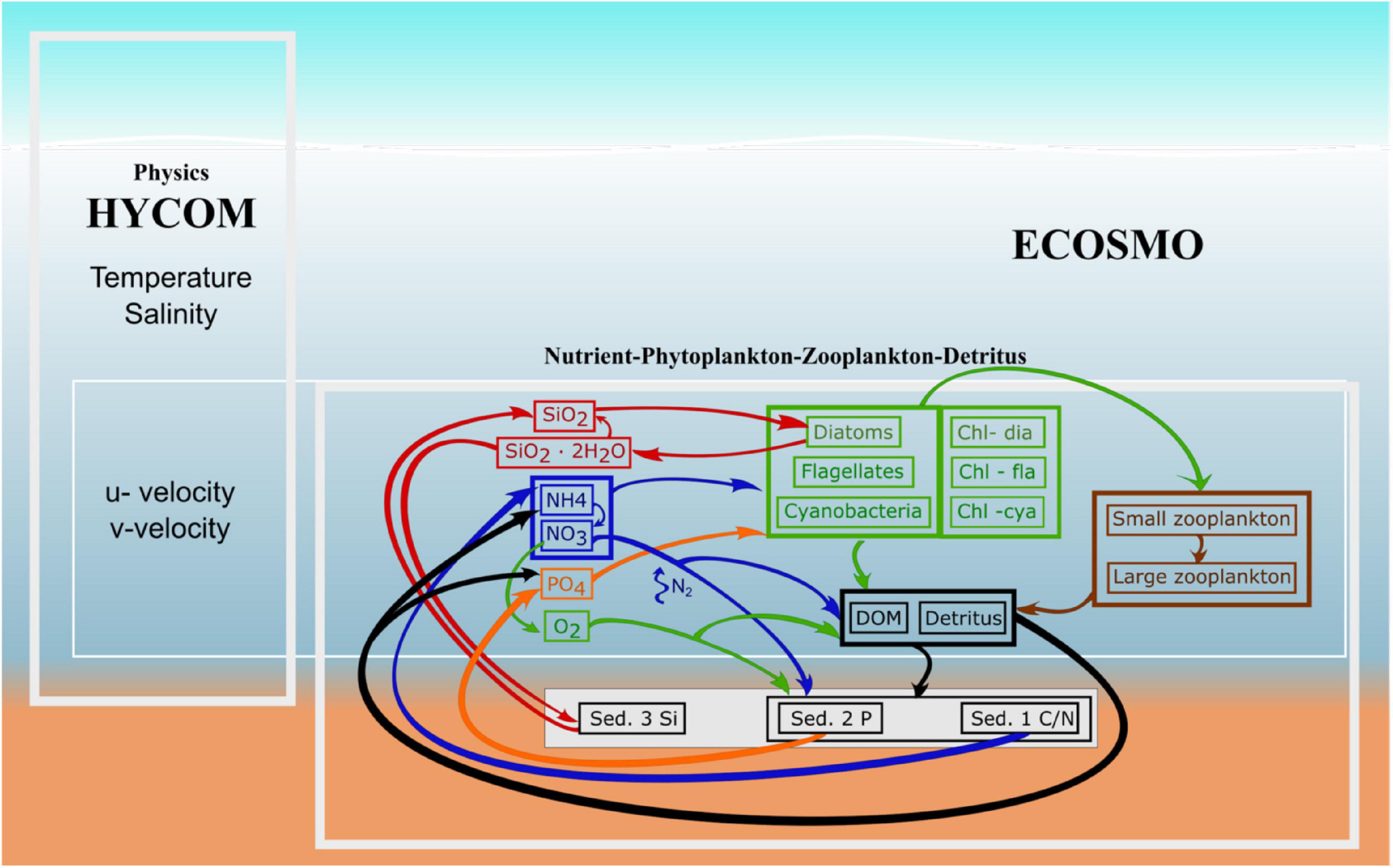
Figure 1. ECOSMO flow chart, showing the model variables and their interactions with each other. The three sediments are Sed. 1, particulate organic sediment, Sed. 2, Iron bound phosphorous, and Sed. 3, the silicate sediment pool.

Among other changes, chlorophyll has been added as a prognostic model compartment. The formulation followed Bagniewski et al. (2011) and the equations for the prognostic state variable for chlorophyll within each phytoplankton type is as follows:

$\frac{\partial {\text{Chl}}_{\text{P}}}{\partial \text{t}}={\mathrm{\rho }}_P{\mathrm{\mu }}_{\text{P}}\text{P}-\sum _{\text{i}=1}^2{\text{g}}_{\text{i}}\left({\text{Chl}}_{\text{P}}\right){\text{Z}}_{\text{i}}-{\text{m}}_{\text{P}}{\text{Chl}}_{\text{P}}$

Here Chl_P is the chlorophyll content of the phytoplankton functional type, where subscript P either represents flagellates or diatoms. The local growth rate of the phytoplankton type is represented by μ_P and P is phytoplankton concentration, either flagellates or diatoms. In the summation symbol i = 1,2 specifies the two zooplankton types (Z_i) and g_i is the zooplankton grazing rate. In the last term m_P is the phytoplankton mortality rate. The phytoplankton-specific photo-acclimation factor, ρ_P, is formulated as follows:

${\mathrm{\rho }}_P=\frac{{\mathrm{\theta }}_{\text{P}}^{\text{max}}{\mathrm{\mu }}_{\text{P}}\text{P}}{{\mathrm{\alpha }}_{\text{P}}\mathrm{PAR}{\mathrm{Chl}}_P}$

where ${\mathrm{\theta }}_P^{max}$ is the maximum chlorophyll-to-carbon ratio, α_P is the initial slope of the photosynthesis-irradiance curve, and PAR is the photosynthetically active radiation. The local ratio is then computed at each time-step taking into account the local irradiance and the predefined range of chlorophyll-to-carbon ratios (given in Table 1). The model then integrates this into the phytoplankton growth and loss terms. With these equations, the model chlorophyll is decoupled from the carbon concentrations, and the chlorophyll-to-carbon ratio can vary with depth, regionally, and seasonally. For example, the model chlorophyll adapts to higher light exposure in summer periods by decreasing the chlorophyll-to-carbon ratio. All parameter values are the same as in Bagniewski et al. (2011), who optimized the model parameters for a site in the North Atlantic. They use a nitrogen-based model, therefore the parameters adopted for chlorophyll_a equations are converted to carbon-units following the classical Redfield stoichiometry.

TABLE 1

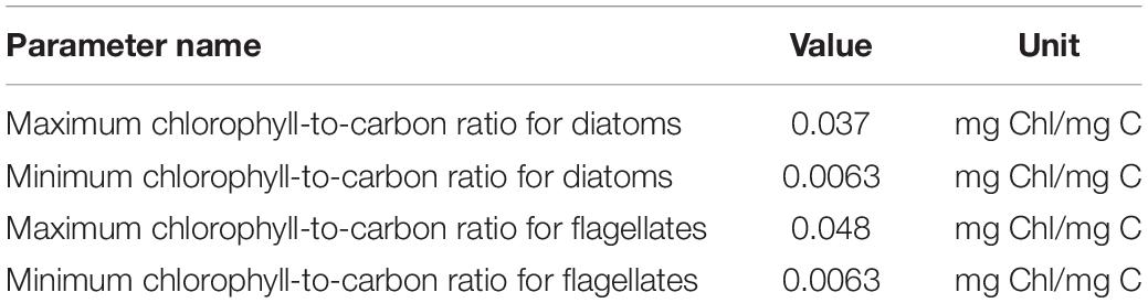
Table 1. Parameters used in the flexible Chl/C-ratio formulation.

The physical model typically has a large influence on the results of biogeochemical models (Skogen and Moll, 2005) and these models often require retuning to produce comparable results after being coupled to a new physical model when used in a different model setup or, more importantly, run for a different region. Therefore, some parameters needed adjustment as part of a tuning that occurred after coupling ECOSMO to HYCOM and changing the modeled region from the North Sea and Baltic Sea to open ocean North Atlantic (Table 2). Some additional changes were implemented in the model after evaluating the result in the lower layers and the sediments. The denitrification rate for sediments was modeled with an exponential temperature dependence in DS2013, where the function worked well because the original model only covered the North Sea and Baltic Sea with only moderate temperature variations among the regions. However, when the model encompasses both the equator and the Arctic, the modeled difference in denitrification rates between the coldest and the warmest region is up to two orders of magnitude (Figure 2). To reduce the difference in denitrification between warm and cold regions, the denitrification rate is now also a function of latitude and temperature, such that the temperature at which this process works at medium efficiency decreases with latitude, while the direct temperature dependency is weaker than in the original model formulation.

TABLE 2

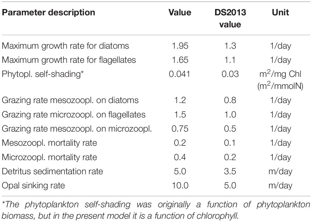
Table 2. The ECOSMO model parameters that have been tuned for HYCOM-ECOSMO compared to those in Daewel and Schrum (2013).

FIGURE 2

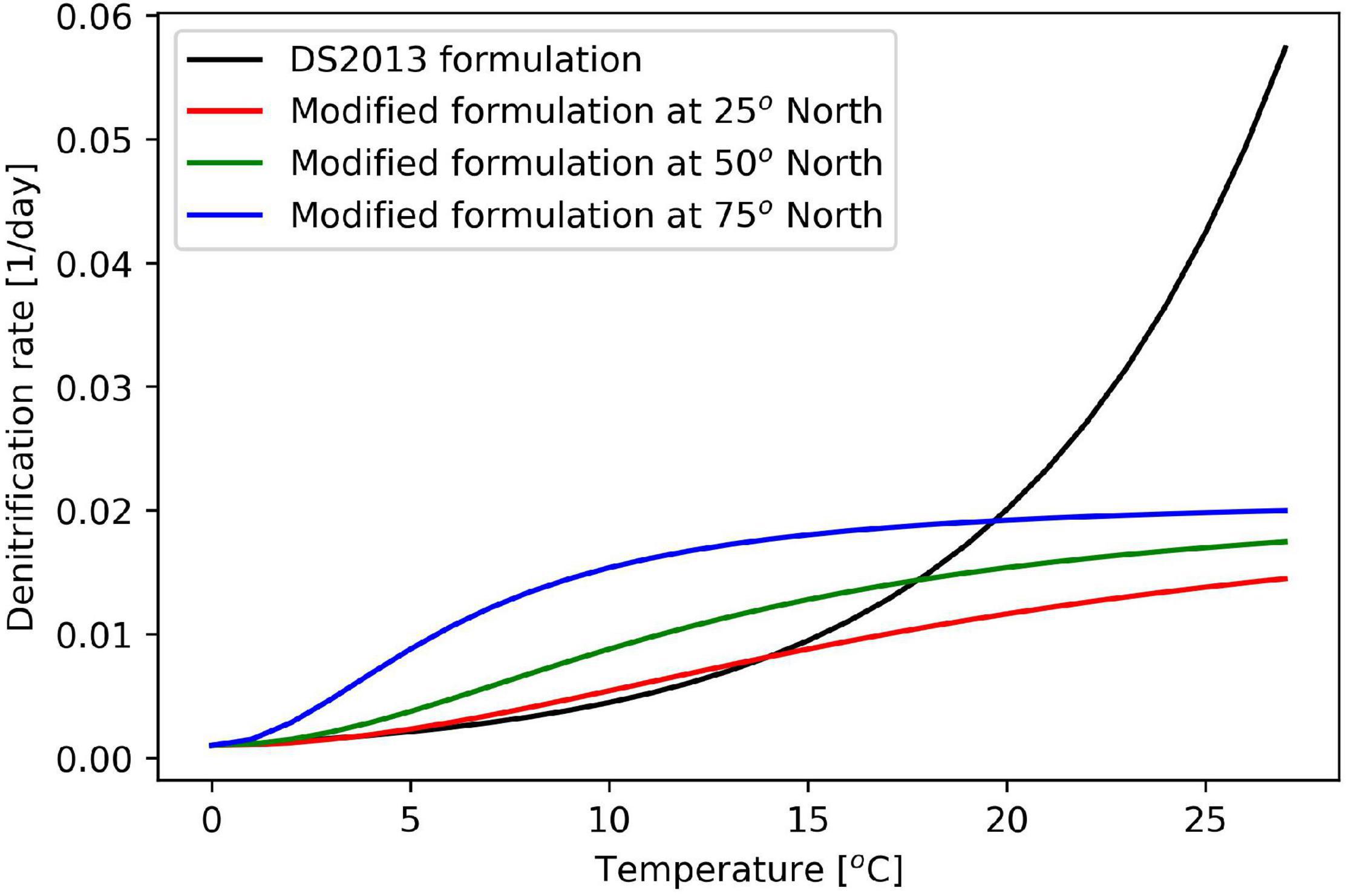
Figure 2. Comparison of original and new formulation for denitrification.

The original formulation for temperature-dependence is as follows:

$Temperature\mathrm{\_}dependenc{e}_{DS2013}=\text{exp}\left(0.15\cdot T\right)$

The modified equation is as follows:

$Temperature\mathrm{\_}dependence=1+20\frac{T^2}{{\left(0.25*lat+25\right)}^2+T^2}$

A comparison of the two formulations is illustrated in Figure 2.

The model did in some cases accumulate large amounts of sediments on the bottom. DS2013 employs a constant burial rate; we have changed this to a burial rate that is dependent on the amount of sediment, that is when there is more sediment present, the burial rate is higher. Sediments are resuspended when the bottom stress is above a certain threshold of 0.007 N/m². The resuspended material is distributed over one or more of the deepest model layers, the criteria being that the layer depths must add up to at least 5 m. This is necessary since the isopycnal layer depths are variable and can range from centimeters to hundreds of meters.

Model Simulation Configuration: Region and Forcing

The simulation was done on a relatively coarse grid that varies between 30 and 70 km and has the highest resolution in mid-latitude in the North Atlantic. Although higher resolution has been shown previously to give better results with respect to nutrients (Samuelsen et al., 2015), the coarse resolution was chosen to make the long-term run feasible computationally and to allow for testing the model with different biogeochemical parameters.

In order to have consistent atmospheric forcing at a reasonable resolution a global high-resolution climate reconstruction based on the atmospheric model ECHAM6 was chosen (Schubert-Frisius and Feser, 2015). This dataset is publicly available and can be downloaded (after registration). The temporal resolution is 1 h, but this was reduced to a 6-h resolution for the dataset that was used to force this model. The dataset has a resolution of about 50 km and surface winds, air temperature, dew-point temperature as well as cloud coverage and precipitation were used to force the physical model. The biogeochemical model also requires input of the part of the short-wave radiation that enters the water column.

River runoff is modeled using a hydrological model, TRIP (Oki and Sud, 1998). The resulting river forcing is a monthly climatology. Hence, this simulation does not include any interannual variability in the river runoff. The river runoff affects the sea water salinity, the river temperature is not included as a forcing in this model. River nutrient loads are derived from the model dataset GlobalNEWS (Mayorga et al., 2010; Seitzinger et al., 2010). Annual discharges of nitrate, phosphate and silicate from different river basins, were used to construct the nutrient river load to force the model. The nutrient loads were scaled by the volume flux of runoff from TRIP, constructing a monthly climatology of nutrient loads.

The model was initialized from climatology, the physical model was spun up from rest and with density fields initialized from climatological values from the Generalized Digital Environment Model (GDEM: Carnes, 2009) fields for temperature and salinity. Initially the physical model was forced with climatological atmospheric forcing for 5 years, and then the model was run for another 4 years with the real-time data from 1948 to the end of 1951, this was repeated 4 times adding up to a total of 21 year spin up for the physical model. The biogeochemical model was initialized from climatology, World Ocean Atlas 2013 for nitrate, phosphate, silicate (Garcia et al., 2013a) and oxygen (Garcia et al., 2013b), while the other biogeochemical variables were initialized from constant low levels. ECOSMO was initialized in the second round of running the model from 1948 to 1951 and in total ECOSMO was spun up for 12 years before initializing the run that is analyzed here.

The sea surface temperature of the model was relaxed toward climatological temperature with a relaxation time scale of 200 days. Furthermore, the boundaries of the model domain that are located between zero and 30 degrees south of the equator, the entrance of the Mediterranean and the Bering Strait were relaxed toward the climatology of temperature, salinity, nitrate, phosphate, silicate and oxygen. Relaxation is strongest at the outer grid cell and is gradually decreased toward the interior of the model over 20 grid cells and the relaxation time scale on the outermost grid cell is 20 days. The climatological datasets used for relaxation are the same as those used for initialization. All the deep-sea variables of the dataset were extracted 1 m above the sea floor.

Validation Dataset

Three datasets were used to evaluate the quality of the model simulation. The first dataset was collected by the Norwegian Institute of Marine Research and contains nutrients, oxygen and pigments from the areas surrounding Norway (Institute of Marine Research, 2018). The dataset can be accessed via the Norwegian Marine Data Centre (NMDC)¹ and include observations from 1980 to 2017. The second dataset was downloaded from the World Ocean Database.² This dataset contains numerous observations of salinity and temperature from both CTDs and XBTs, and in addition this dataset contains some oxygen observations. Finally, the dataset GLODAPv2 Bottle data (Olsen et al., 2016) was used, this dataset contains nutrients, hydrography and variables related to carbon chemistry. The three datasets are hereafter referred to as NMDC, WOD, and GLODAP. Very few observations are obtained immediately above the bottom, to only evaluate the deepest water masses, only observations collocating with the deepest layer of the model was included in the validation.

Study Site

In this work, we have focused on regions known to host suitable habitat for sponges of the family Geodiidae, which are often a key constituent of boreo-Arctic-type sponge grounds (Klitgaard and Tendal, 2004; Cárdenas et al., 2013) and which are emerging as being amongst the more studied deep-sea sponges with better known distributions. We have selected areas corresponding to four of the study sites identified in Roberts et al. (2021a) and focused our investigation of interannual variability on these known sponge habitats. The regions are the Flemish Cap (FLC) off the east coast of North America, the Reykjanes Ridge (RYR) to the south of Iceland, the North Norwegian Shelf (NNS) off the coast of Norway and the East Greenland Shelf (EGS) off the northeast coast of Greenland (Figure 3). These sponge habitats were selected because they represent good geographical coverage of the North Atlantic and a diversity of hydrographic settings. They are also far enough away from the lateral boundaries of the model domain to not be directly influenced by the relaxation to climatology, and in three cases (FLC, RYR, and NNS) hydrographic observations were available with which to evaluate model performance.

FIGURE 3

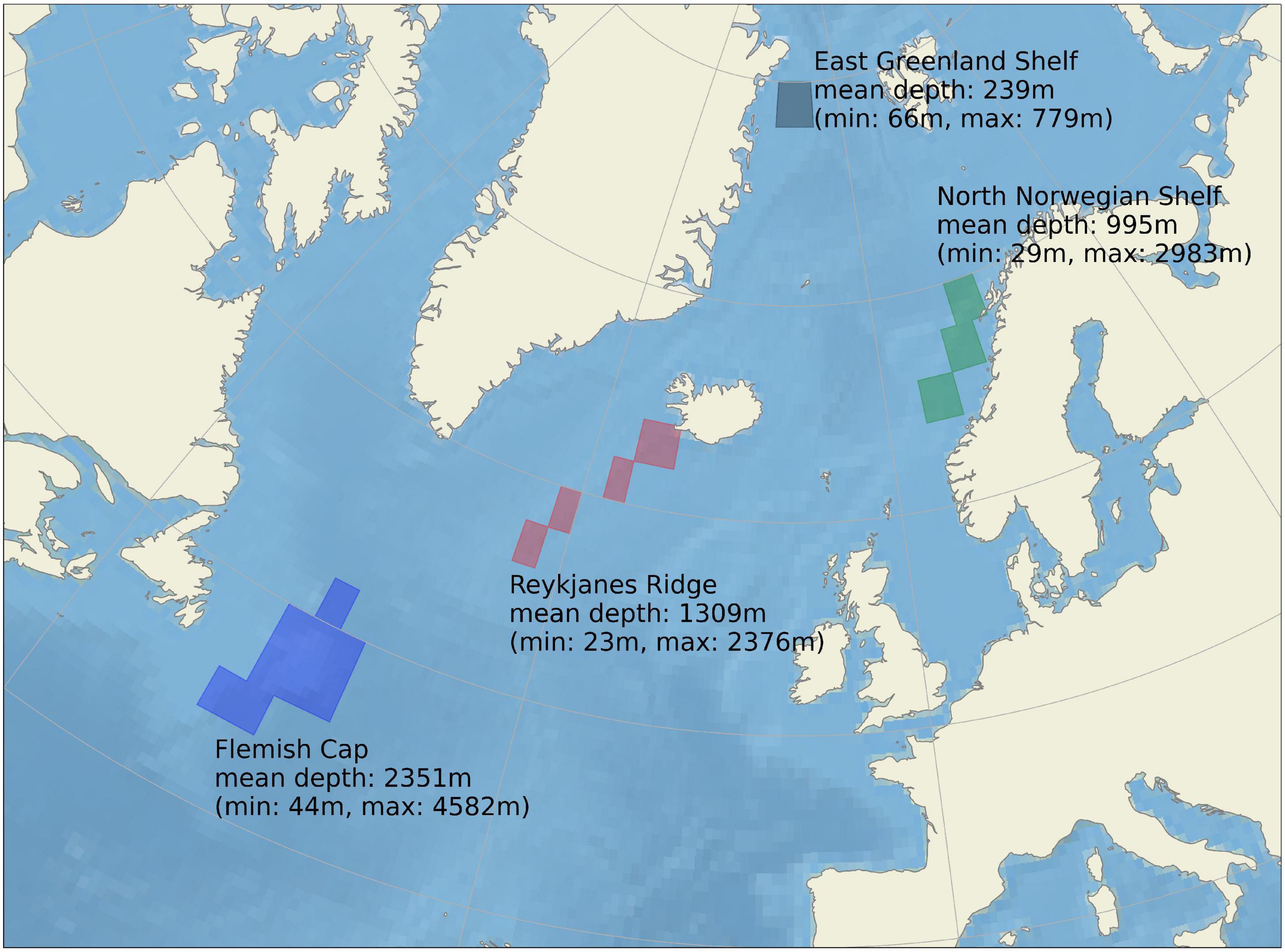
Figure 3. The four areas of sponge habitat that are the focus of this paper. The minimum, maximum and mean depth for each study site based on the model bathymetry, are shown together with the geographical extent.

The Flemish Cap is a shallow bank off the continental shelf of eastern Canada. It is about 200 km across and at the shallowest it is about 150 m. The deep-sea sponge community composition in the area is typically of boreal type, being dominated by astrophorids (Geodia spp., including Geodia atlantica, Geodia barretti, Geodia macandrewii, Geodia phlegraei) and Asconema sp., although some colder-water species are found at greater depths. The largest concentrations of sponges are found along the slopes of the bank (Murillo et al., 2012). The water masses at FLC consist of Labrador Current Slope Water (LCSW) with temperature of 3–4°C and salinities of 34–35 and Atlantic Water coming from the south from the North Atlantic Current, typically warmer than 4°C and with salinities greater than 34.8 (Colbourne and Foote, 2000).

The Reykjanes Ridge is located to the south of Iceland and is a part of the mid-Atlantic ridge. The landscape is rocky ground (although soft substrata also occur) and the depth ranges from about 500 to 2,000 m. The water masses at intermediate depth at RYR include Subpolar Mode Water which is about 6°C in the RYR area, and is characterized by high oxygen levels because of its recent contact with the atmosphere (Petit, 2018). There is also Labrador Sea Water with temperature around 3°C and salinities around 34.8 (Fröb et al., 2018) and in deeper layers dense (> 27.8 kg m^–3) and saline (> 34.98) Iceland-Scotland Overflow Water (ISOW) originally formed by deep convection (Petit, 2018) and a mix of ISOW and the overlying Atlantic water known as Icelandic Slope Water (Yashayaev et al., 2007). Sponge communities at RYR are characterized by demosponges of the genera Geodia and Phakellia, together with Poecillastra compressa, and by hexactinellids such as Aphrocallistes beatrix and Asconema spp. (Copley et al., 1996; Kuznetsov and Detinova, 2001; Cárdenas and Rapp, 2015). Whilst the sponge communities at RYR are also largely boreal in type, being dominated by, for example, G. atlantica, G. barretti, G. macandrewii, G. phlegraei, the occurrence of strict Arctic species (Geodia hentscheli, Stelletta rhaphidiophora) is reported, likely because of the influence of Iceland-Scotland Overflow Water along the flanks of the ridge (Cárdenas and Rapp, 2015).

In the offshore area of the North Norwegian Shelf upper water masses are North Atlantic Water and Norwegian Coastal Water, typically separated by being above and below salinity of 35.0. The water on the continental shelf edge (200–300 m) is primarily North Atlantic Water, typically in the range 6–8°C with the warmest temperatures in the fall (Skarðhamar et al., 2005). In the deeper layers there are Norwegian Sea Arctic Intermediate Water of 0.5 to –0.5°C and Norwegian Sea Deep Water (< –0.5°C) (Buhl-Mortensen et al., 2012). The depth in this region ranges from 100 to 3,000 m. Sponge grounds in this area are of boreal type and are dominated by assemblages of astrophorids (genera Geodia, Stryphnus, and Stelletta) (Buhl-Mortensen et al., 2009; Hogg et al., 2010).

The East Greenland Shelf is the shallowest of the regions we are investigating, located mostly on the shelf off northeast Greenland, with a maximum depth of about 800 m. The region is covered by sea ice most of the year and therefore has low primary production. The water masses are Polar Surface Water exiting the Arctic, about –1°C, and salinity as low as 30 on the surface and increasing to 34.5 toward the bottom (de Steur et al., 2009). The area can also be influenced by recirculating Atlantic water from the Fram Strait (Rudels et al., 2002). Sponge assemblages in this region are of Arctic, or cold-water, type, and are composed of the tetractinellids G. hentscheli, G. parva, S. rhapidiophora and Thenea valdiviae, together with the hexactinellids Schaudinnia rosea, Trichasterina borealis, Scyphidium septentrionale, and Asconema foliatum (Klitgaard and Tendal, 2004).

Time Series Extraction

From the original dataset of 0.1° resolution we constructed a monthly time series from each region by spatially averaging over each region (Figure 1), distinguishing between regions with bottom depth 200–700 m and areas deeper than 700 m. There was an increasing trend of both silicate and nitrate at all the sponge grounds investigated that have no corresponding trend in the observational datasets used (see model evaluation section below). Therefore we present the nitrate and silicate time series with the linear trend removed, retaining only the annual cycle and the interannual variability. Because of the relatively coarse grid used in the simulation, the depth given in Figure 3, which is extracted from the model bathymetry is not always consistent with the depths given in the literature for these sponge habitats.

Results

Model Evaluation at the Selected Sponge Habitats

The region used for validating FLC is larger than the area used in this paper and stretches further north along the coast of Canada. There were more than 1,000 hydrographic observations from WOD which showed that the model had a warm bias of about 1°C and a salinity bias of 0.15. There was a limited number of observations from GLODAP that resulted in a similar temperature bias, but a smaller salinity bias of 0.05. A potential cause of this warm bias in this region is the late separation of the Gulf Stream which is a common problem in numerical ocean models (Ezer, 2016). In this region, the modeled oxygen ranged from 4.5 to 8 ml/l, but the observed oxygen was more stable, ranging between 5.5 and 6.5 ml/l. Silicate had a positive bias of about 3 mmol/m³, phosphate a small negative bias and the simulated nitrate was overall very good. There were only about 50 nutrient observations available for the whole time period. At the RYR there were only about 50 hydrographical observations that yielded a cold bias of about 0.6°C and a salinity bias of only 0.03. The North Norwegian Shelf had the largest number of observations (> 2,500) of the three regions. The analysis yielded a fresh bias of 0.18 and a cold bias of 1.18°C. At the NNS the model produces a positive trend of all three nutrients that is not present in any of the datasets that we compare to. In the EGS we found no observations for model comparisons and thus cannot provide an evaluation of the model performance in this region. The error statistics FLC, RYR and NNS are summarized in Supplementary Tables 1–3, and an evaluation of the model applied to sponge habitats throughout the North Atlantic can be found in Samuelsen et al. (2019).

Mean Conditions and Annual Cycle

In the following we report on the areas, differentiating between areas where the bathymetry is between 200 and 700 m and deeper than 700 m. Areas with bathymetry above 200 m have not been analyzed. Where nothing else is stated, the main value given is from the upper region and the number in parentheses is from the deeper region. These deeper areas are characterized by relatively stable conditions year-round. However, clear annual cycles still emerge (Supplementary Figures 1–4). The three mid-latitude sponge habitats (FLC, RYR, NNS), are colder and fresher during spring and warmer and saltier during the autumn. At the Flemish Cap, the mean temperature is 7.7°C (2.8°C) with a range of 0.8°C (0.04°C) and salinity varies from 34.88 to 34.98 and a range of 0.003 in the deeper layers. The temperature range at the RYR and NNS are 0.7°C (0.07°C) and 0.2°C (0.08°C), respectively, but on average the RYR is warmer with 6.0°C (4.9°C) compared to 4.8°C (0.03°C) at NNS. The salinity variations are only 0.02 at RYR and 0.04 at NNS over the annual cycle. In the EGS, the temperature variation is about 0.03°C, while the range of salinity is 0.01, with the most saline water in the autumn, potentially the retraction of sea ice from the area allows for the intrusion of more saline waters from the Fram Strait.

Similarly, nutrients and oxygen have small annual variations. Nutrients are higher in the autumn than in the spring at all the sponge habitats, but the variations are likely too small to influence the sponges. All sponge areas are quite well oxygenated with oxygen levels of 6 ml/l or above, except above 700 m at FLC where the mean is 5.2 ml/l. RYR has the largest annual cycle of oxygen of only 0.26 ml/l, with minimum in the autumn. Variations in the oxygen levels at these selected sponge habitats are quite closely the inverse to variations in temperature, therefore oxygen at the sponge grounds can potentially be predicted quite well by the change in temperature. Such close relationships between temperature and oxygen are common in deeper water masses as cold water can dissolve more oxygen, though the dissolved oxygen declines due to remineralization with time away from the surface. In the model mean state distribution of bottom oxygen (not shown) there are areas of low oxygen ∼2 ml/l at the bottom of the Baffin Bay and in the Gulf of St. Lawrence, but these low-oxygen waters do not intrude into other regions. The nitrate-to-silicate ratio decreases as the presence of Arctic water of Pacific origin becomes more prevalent, is above 1 at the NNS, about 1 at RYR and below 1 at FLC and in the EGS, but it should be kept in mind that where we have observations the model overestimates the silicate concentration.

At the FLC the flux of detritus to the sea floor is at a minimum in February and peaks in August, 2 months after the maximum secondary production. The detritus flux stays relatively high until October. At the other 3 sponge habitats the minimum occurs between April and June, with the maximum in September/October. The factors playing a role here are the depth of the sponge habitats and the progression of the phytoplankton bloom and corresponding zooplankton growth from south to north over the season. Because of the low productivity in the EGS the downward flux of detritus is only around 5. mgC/m²day, only about 2–10% of the influx of particulate organic matter at the other sponge habitats. Below 700 m, the detritus flux is low and even.

Long Term Trends and Interannual Variability

Looking at annual means of the model variables over the simulation period at the sponge habitats (Figures 4–7), the three southernmost sponge regions have temperature ranges of about 5.9°C (0.9°C) at FLC, 1.1°C (0.7°C) at RYR, 1.1°C (0.5°C) at NNS, and 0.5°C (0.4°C) at EGS. The salinity range was 0.5 at FLC, less than 0.1 at NNS and RYR, but 0.2 in the EGS. The strongest temperature trend is a cooling trend of –0.53°C per decade at the Flemish Cap above 700 m (Table 3) accompanied by a very small freshening (Table 4). A closer inspection of the timeseries of temperature and salinity (Figure 4A) shows that there are three large intrusions of cold, fresh waters, most likely of polar origin in the mid-1990s, 2000s, and 2010s. The intruding water is about 4°C colder and 0.2 fresher than normal. At RYR (Figure 5) and NNS (Figure 6) there are positive temperature trends of 0.06°C above 700 m and 0.08°C below 700 m, respectively (Tables 3, 5). This is accompanied by a small increase in salinity at RYR, but a very small freshening trend in the NNS. At RYR there is a relatively stable increase in temperature and salinity over the whole simulation period, while at NNS there is cooling in the 1970s and 80s and warming in the 90s. Unlike at the other sponge habitats, the salinity and temperature at NNS have periods in the 1960s and late 1990s when the change is out of phase, i.e., there is a fresh and warm water mass. At both these sponge habitats the simulated temperature has a similar warming trend to the observations. At EGS the temperature trend is very small, but there are fluctuations with warmer and more saline waters in the 70s, 80s and 2000s that last for about 5 years each (Figure 7). Anomalous conditions, defined as values more than two standard deviations away from the mean (red stars in Figures 4–7), occur primarily at the beginning or end of the timeseries, except for NNS that has a fresh period in the 1980s.

FIGURE 4

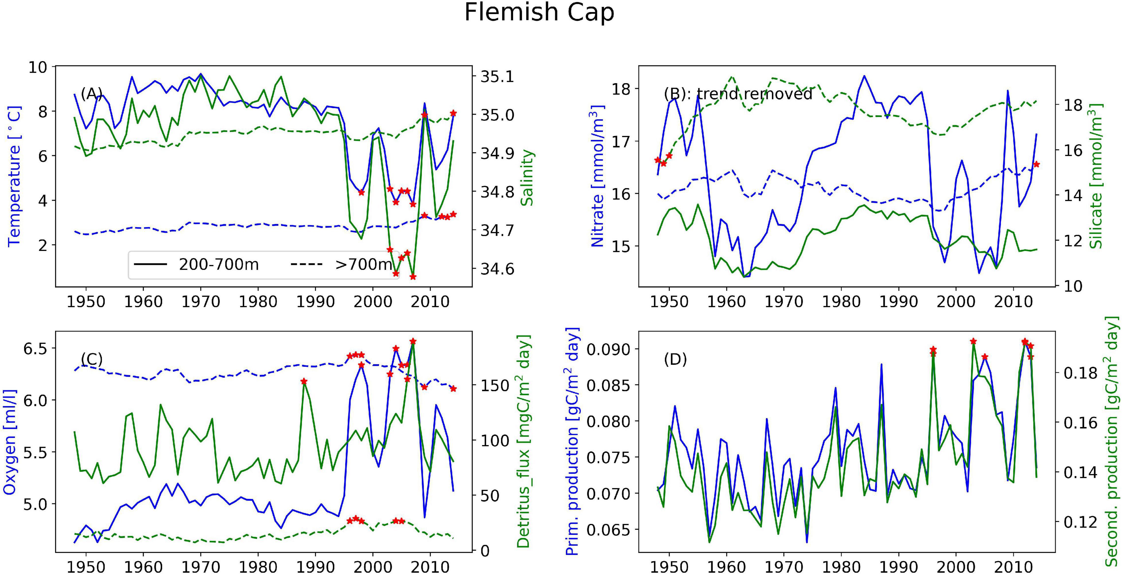
Figure 4. Timeseries of the annual mean of different variables illustrating the interannual variability at the Flemish Cap for (A) temperature (blue) and salinity (green), (B) nitrate (blue) and silicate (green), and (C) oxygen (blue) and detritus (green). Solid lines are areas with bottom depth between 200 and 700 m, dashed lines are areas deeper than 700 m. (D) Depth-integrated primary production (blue) and secondary production (green) from the full area. Red stars indicate years when values are outside two standard deviations of the temporal mean.

FIGURE 5

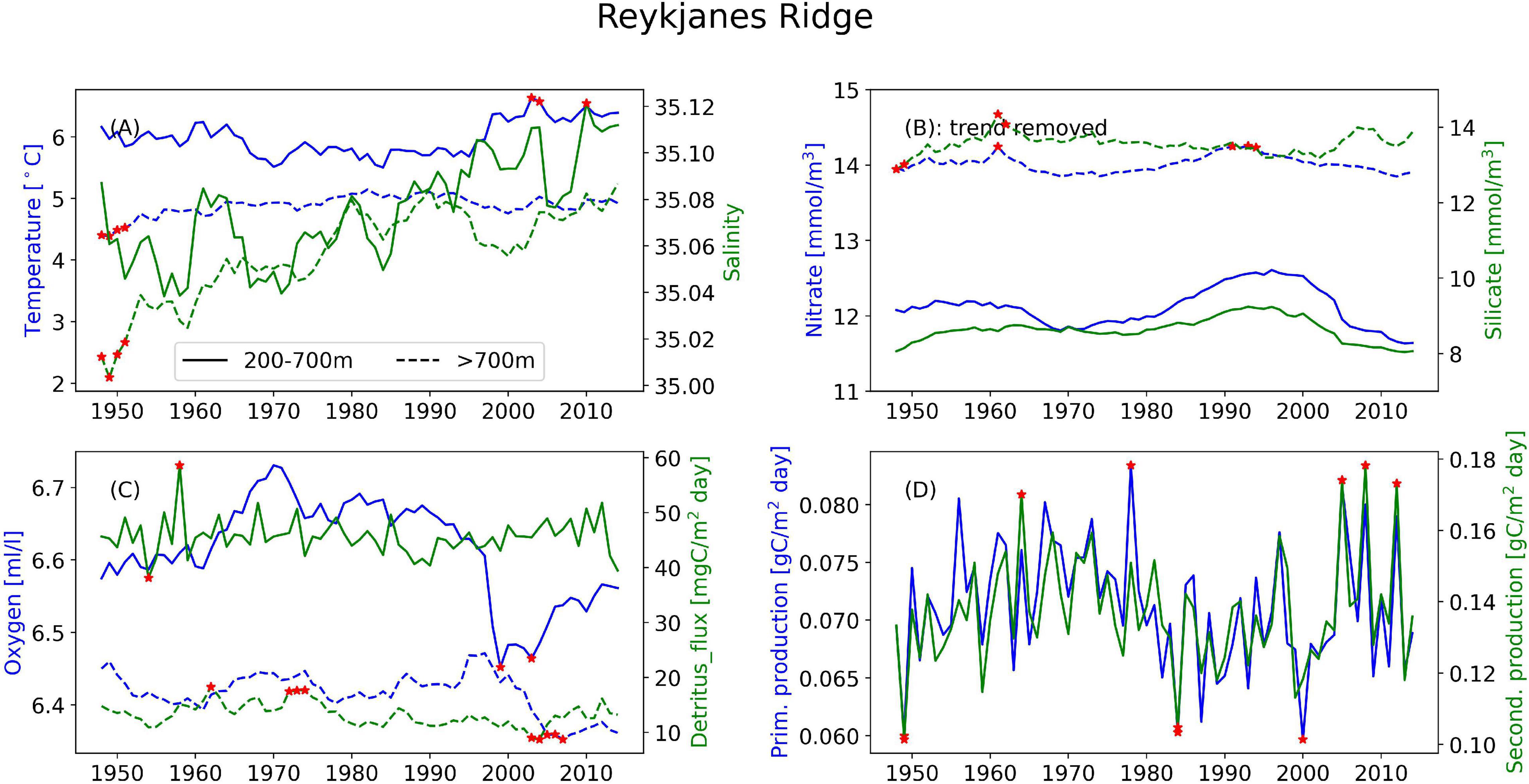
Figure 5. Timeseries of the annual mean of different variables illustrating the interannual variability at the Reykjanes Ridge for (A) temperature (blue) and salinity (green), (B) nitrate (blue) and silicate (green), and (C) oxygen (blue) and detritus (green). Solid lines are areas with bottom depth between 200 and 700 m, dashed lines are areas deeper than 700 m. (D) Depth-integrated primary production (blue) and secondary production (green) from the full area. Red stars indicate years when values are outside two standard deviations of the temporal mean.

FIGURE 6

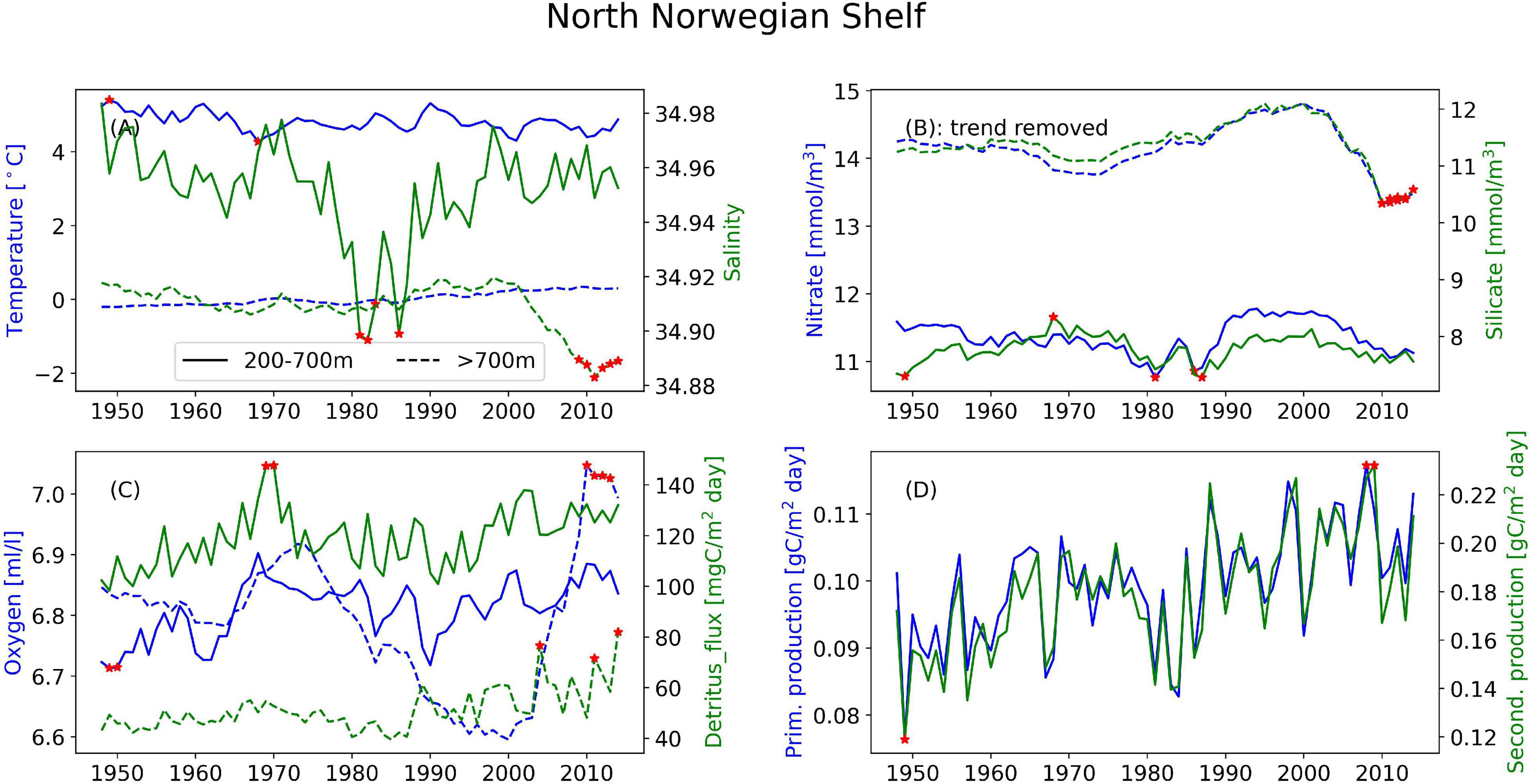
Figure 6. Timeseries of the annual mean of different variables illustrating the interannual variability at the North Norwegian Shelf for (A) temperature (blue) and salinity (green), (B) nitrate (blue) and silicate (green), and (C) oxygen (blue) and detritus (green). Solid lines are areas with bottom depth between 200 and 700 m, dashed lines are areas deeper than 700 m. (D) Depth-integrated primary production (blue) and secondary production (green) from the full area. Red stars indicate years when values are outside two standard deviations of the temporal mean.

FIGURE 7

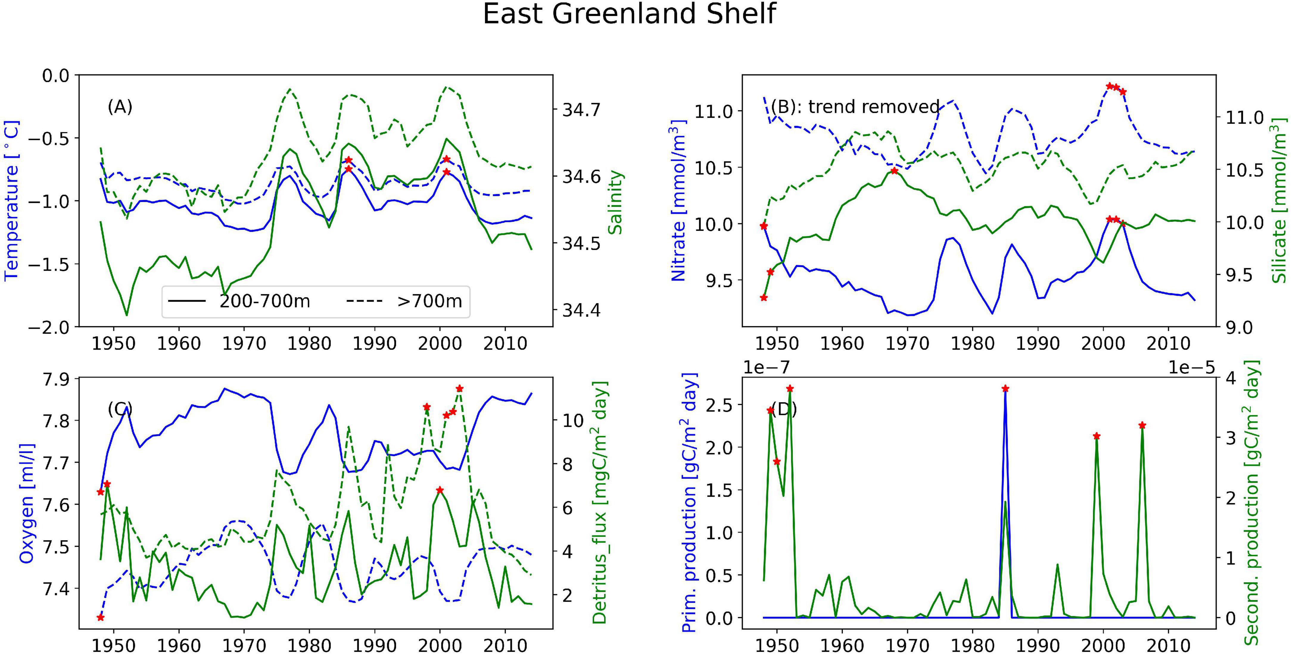
Figure 7. Timeseries of the annual mean of different variables illustrating the interannual variability at the East Greenland Shelf for (A) temperature (blue) and salinity (green), (B) nitrate (blue) and silicate (green), and (C) oxygen (blue) and detritus (green). Solid lines are areas with bottom depth between 200 and 700 m, dashed lines are areas deeper than 700 m. (D) Depth-integrated primary production (blue) and secondary production (green) from the full area. Red stars indicate years when values are outside two standard deviations of the temporal mean.

TABLE 3

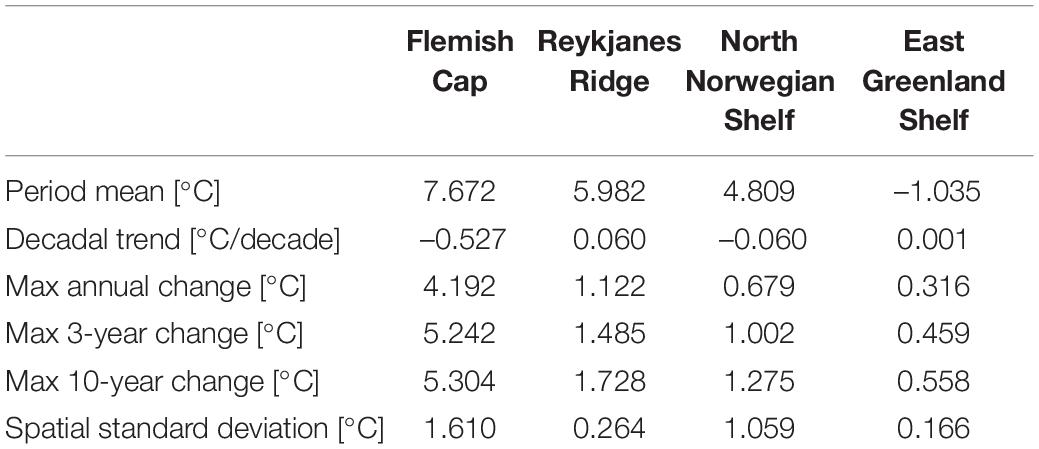
Table 3. Summary of temperature properties at the four sponge habitats in waters with bottom depth 200–700 m: Period mean, decadal trend, the maximum change in the monthly mean over a period of 12, 36 months, and 10 years, and the temporal mean of the spatial standard deviation.

TABLE 4

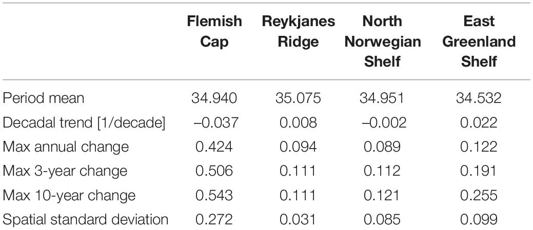
Table 4. Summary of salinity properties at the four sponge habitats in waters with bottom depth 200–700 m: period mean, decadal trend, the maximum change in the monthly mean over a period of 12, 36 months, and 10 years, and the temporal mean of the spatial standard deviation.

TABLE 5

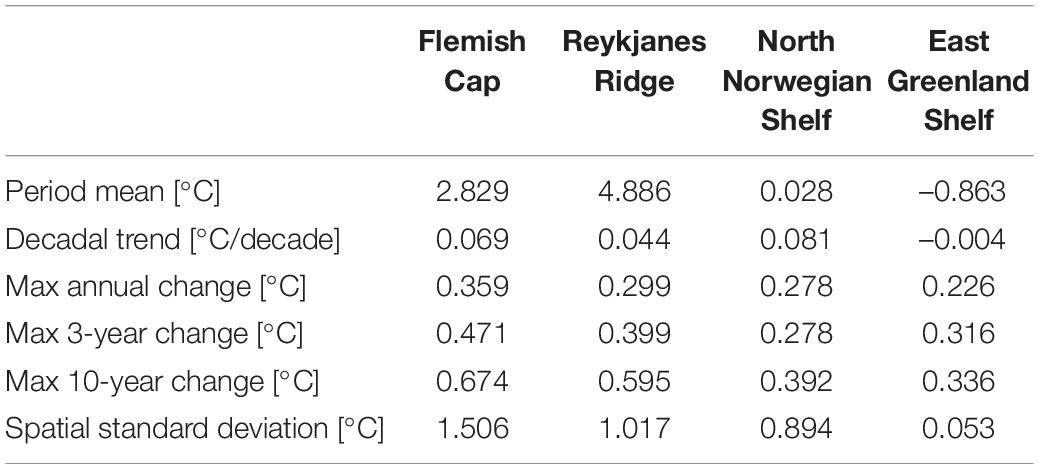
Table 5. Summary of temperature properties at the four sponge habitats areas with bottom deeper than 700 m: Period mean, decadal trend, the maximum change in the monthly mean over a period of 12, 36 months, and 10 years, and the temporal mean of the spatial standard deviation.

Nitrate and silicate are increasing over the model period at all four sponge habitats over the simulation period, however, from the comparison to observations, we believe these trends are a model artifact, thus the timeseries shown in Figures 4–7 have been detrended and no trends are presented for these variables. When the trend is removed, all four sponge habitats show an interannual variability of both nutrients of O(1 mmol/m³). From the monthly timeseries the largest occur above 700 m at the FLC with > 4 mmol/m³ nitrate and >4 mmol/m³ silicate over a 10-year period (Supplementary Tables 4, 6). At FLC and EGS there are variabilities in nitrate on a timescale from 3 to 10 years, at RYR and NNS the variability is multi-decadal. The variability of silicate is more multidecadal in nature at all four locations and has a similar long-term variability to nitrate at FLC and NNS (Figures 4, 6). Anomalous conditions occur in both depth ranges, lower nutrients in the deeper part of the water masses occur at NNS and coincide with a freshening, in the last 5 years of the simulation.

The oxygen at FLC shows an increasing trend of 0.17 ml/l/decade (Supplementary Table 8) above 700 m while the remaining habitats have low oxygen trends. At FLC and NNS the detritus flux increases by 3.9 and 2.4 mgC/m² day/decade, respectively (Supplementary Table 10). Detritus fluxes at the sponge grounds exhibit year-to-year variations, while oxygen exhibit slower, multi-decadal variations. Above 700 m, on longer time-scales the higher flux of detritus is associated with higher oxygen concentration in the waters at FLC, RYR and NNS (Figures 4–6), while at the EGS oxygen and detritus flux have an inverse relationship (Figure 7). At EGS the deeper detritus flux exceeds the shallower region. Anomalous high values occur most often in the deep regions in the 1990s and 2000s at FLC and EGS and in the 1970s and 2000s at RYR.

For primary and secondary production, we did not distinguish between depths as this made very little difference for these variables. Primary and secondary production (Figure 4–7D) vary in a seemingly unrelated way to the changes in the deep sea. The interannual variability of primary and secondary production follow each other very closely. At FLC and NNS there is a slight [O(2.0 × 10^–3) gC/m²day/decade] positive trend of primary production over the simulation period. This is potentially related to increasing nutrient concentrations, but warming could also play a role as growth is more efficient at higher temperatures. Anomalous years occur toward the end of the period at FLC and NNS, and intermittently throughout at the two other sponge habitats.

On interannual timescales there are co-variabilities between the water-masses and the biogeochemical properties at FLC and EGS. Nitrate co-varies with large fluctuations in the water masses in the EGS where the relationship is strongest with temperature (r = 0.9), and FLC where the relationship is strongest with salinity below 700 m (r = 0.79). Additionally, oxygen has a strong inverse relationship (r < –0.9) with temperature below 700 m at these sponge habitats. The detritus flux is also connected to water masses where higher-temperature water is associated with more detritus flux (r = 0.67) at EGS and colder water is associated with more detritus flux (r = –0.8) at FLC below 700 m. At FLC the two intrusions of colder fresher water mass are accompanied by an increase in oxygen and detritus flux beyond what is simulated by the model in the period before (Figure 4). This oxygen-rich water mass is LCSW originating from the north on the shelf off Canada. Visual inspection of animations of the model results showed that the southward extension of this water mass is an annual event on the areas inshore of the Flemish Cap, but only in the later years does it extend west onto the Flemish Cap. The three warm peaks in the EGS are accompanied by increased detritus flux, but no corresponding increase in the local biological production is seen. Simultaneously there are temporary decreases in oxygen. The above indicates that these may be a result of advection of water masses from further east in the Fram Strait which are warmer, saltier and with a higher concentration of detritus. The absolute variability of temperature is 0.3°C while the detritus flux to the sea floor increases sixfold during the “warm” periods, although the absolute value is also very low. Oxygen and nitrate have a strong negative relationship of (r < –0.8) at both these sponge habitats.

At NNS and RYR water masses and the biogeochemical variables are not so tightly connected. Also here oxygen is negatively correlated to temperature, by r = –0.87 at RYR and r = –0.92 at NNS, above 700 m. Below 700 m, no correlation could be found. The strongest relationship is found between oxygen and nutrients (r > –0.97) at NNS below 700 m.

Discussion

There are numerous deep-sea sponge habitats across the North Atlantic Ocean. At selected sponge habitats there are short-term monitoring timeseries (e.g.,Hanz et al., 2021b), at others physical ocean reanalysis products have been used to study the conditions (Beazley et al., 2018). However, at most sponge habitats long-term monitoring time series are missing. Here, we present a coupled physical-biogeochemical model hindcast of the North Atlantic covering the period from 1948 to 2014. To our knowledge, this is the first time such a model hindcast has been produced specifically with the aim of representing environmental conditions at deep-sea sponge habitats.

The purpose of this study is to use the model hindcast to investigate the mean conditions and long-term variability at sponge habitats over the last half century. Whilst outputs from ocean models can be used in species distribution modeling (SDM) approaches to predict distributional shifts and answer biogeographical questions (e.g., Beazley et al., 2021), and the dataset generated here has similar utility, in this work we extract timeseries data across a suite of environmental variables at known sponge habitats with a view to informing a baseline understanding of conditions experienced by extant populations in the recent past. It is generally thought that the deep sea, below the permanent thermocline, provides a relatively stable environment for the organisms living there and therefore it is possible that these organisms may not be able to acclimatize to abrupt changes in their environment. However, the sensitivity of sponges to changes in the environment is poorly known. One experiment (Strand et al., 2017) suggested that deep-sea boreal sponges were quite resilient to temperature increase alone, but may be sensitive to multiple stressors such as a simultaneous warming and decreasing oxygen concentrations. However, G. Barretti in the Skagerrak suffered mass mortality after being subjected to abrupt advection of warmer water (Guihen et al., 2014). Bell et al. (2018) found that sponges appear to be less sensitive to warming than other benthic taxa and may therefore emerge as a winner under climate change, although the work had a focus on shallow-water sponges in various settings (rather than North Atlantic/Arctic deep-sea sponges, as considered here). For shallow sponges, it was found that they were more tolerant to warming than corals, but a large warming, such as that in the RCP8.5 climate change scenario, would harm the sponge population (Bennett et al., 2017). Another study found that one species of coral and one species of sponge coming from a Norwegian fjord reacted negatively to heating and suspended sediment, but the coral was more sensitive (Scanes et al., 2018). Work from the Northwest Atlantic has shown that deep-sea sponge grounds may have persisted in the face of considerable environmental variability over 100s–1000s of years (Murillo et al., 2016; Beazley et al., 2018).

From the timeseries analyzed we identified that abrupt changes to the water masses could occur. At FLC above 700 m the temperature changes by more than 4° over just 1 year and at EGS the change was 0.31°C which is large compared to the mean annual range of 0.03°C. These abrupt changes were accompanied by changes in salinity, oxygen and detritus flux to the seabed as well. This is new information for 3 of the 4 sites selected (RYR, NNS, EGS). Whilst the magnitude of the fluctuations is relatively small, these results can help inform future studies of sponge sensitivity to environmental change. We assume that because any large/mature specimens collected in these areas in recent times (Roberts et al., 2021b) likely represent individuals of many decades to centuries in age (Prado et al., 2021), they appear to have persisted despite this level of variability.

The distribution of certain species of sponges is connected to specific water masses (Klitgaard and Tendal, 2004; Roberts et al., 2021a) and they likely have preferred ranges of environmental variables, connected to optimal growth conditions, feeding and the spreading or retention of larvae. Sponges are mainly slow-growing, and where they have been physically removed, for example by bottom trawling, it may take several decades to re-establish the population (Morrison et al., 2020). Any loss of sponge habitat to environmental change could potentially have large consequences for deep-sea ecosystems, in terms of the loss of hotspots of biodiversity, stepping stones of connectivity, and nutrient cycling (Hogg et al., 2010), and if the environment changes permanently this would likely inhibit recovery. Therefore, one of the main contributions of this study is to establish the mean conditions and range of variability seen by deep-sea sponges in the past, so that as new data on sponge sensitivity to environmental change becomes available, we can evaluate whether conditions are moving beyond species’ ecophysiological tolerances.

We observe both trends and interannual variations in the environmental conditions at the deep-sea sponge habitats investigated here. The magnitude of the fluctuations are generally small and that is reflected both in the annual cycle at each of the sponge habitats (see Supplementary Figures 1–4) and the interannual timeseries (Figures 4–7). The seasonal cycle at the sponge habitats investigated fluctuates with less than 1°C over the season and in the East Greenland Shelf the seasonal fluctuation is < 0.1°C. Seasonal fluctuations in salinity are similarly small. Nitrate and silicate vary by < 1 mmol/m³ and though there are clear seasonal cycles in oxygen, the range of the annual cycle is < 0.3 ml/l. The interannual variability present in the model will either be caused by variability present in the atmospheric forcing used or internal dynamics within the ocean-biogeochemical system. Given that the sponge habitats are present at several hundred meters depth, the impact from the forcing will not be immediate and can take several years to reach these depths, depending on the area. At the RYR there is a gradual warming of the water masses and there are warming trends at both NNS and EGS. This is most likely the result of the warming present in the atmospheric reanalysis forcing. There is also a positive trend of surface primary production at the FLC and the NNS. This can be either due to increased growth at increased temperature or increased availability of nutrients. The timeseries constructed here have been averaged over a large range of depths which would smooth the variability and it is therefore likely that the local variations are larger than the averaged ones reported here. The mean spatial standard deviation is a measure of the spatial variability in the region (Tables 3–6 and Supplementary Tables 4–11). Typically, the temporal fluctuation, on a monthly timescale, is larger than the spatial variability above 700 m and smaller than the spatial variability below 700 m.

TABLE 6

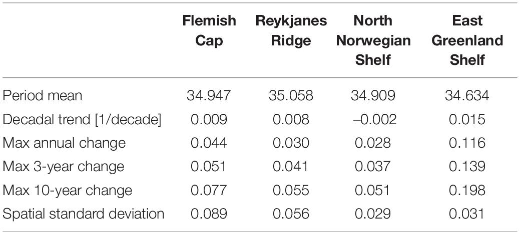
Table 6. Summary of salinity properties at the four sponge habitats in areas with bottom deeper than 700 m: Period mean, decadal trend, the maximum change in the monthly mean over a period of 12, 36 months, and 10 years, and the temporal mean of the spatial standard deviation.

When water masses exist in close vicinity of each other and shift in space, it can manifest locally as a large environmental change happening over a short time. Such variations from shifts in water masses are most likely the cause of the fluctuations with duration of 4–6 years of about 4°C at FLC (Figure 4) and 0.3°C at EGS (Figure 7). At FLC, the water mass variability in the last two decades is visibly different from the variability of the first four decades (Figure 4), and is characterized as anomalous in several years during the 2000s. This area is influenced by North Atlantic waters, but also LCSW. The intrusion of colder, fresher water is similar to that reported on in Colbourne and Foote (2000) who analyze observations from 1960 to 1996, but the cooling periods they report on do not coincide temporally with the model. The two earliest periods occurring in the 1970s and 1980s, were attributed to anomalously low heat flux, while the period in the 1990s, was attributed to advection. From the model result it seems that changes in the Arctic may facilitate more frequent occurrences of colder, more productive water masses on the Flemish Cap. The accompanying increase in detritus flux from this water mass will increase the food availability to the sponges. The East Greenland Shelf area is relatively shallow, but being covered by sea ice for most of the year it has been protected from the direct forcing of the atmosphere. However, the second half of the hindcast period showed more variability. It is therefore likely that the simulated changes in the later period at both these sponge habitats can be connected to loss of sea ice thickness and extent in the Arctic Ocean (Stroeve et al., 2012; Ivanova et al., 2014; Onarheim and Årthun, 2017) that exposes the ocean to more direct atmospheric forcing and eventually influencing the regions downstream of the Arctic.

Changes in the biogeochemistry occur by a more direct route than changes in physical variables, that is via the sinking of organic material which propagates faster vertically in the ocean than physical properties. The hindcast shows that there can be very large variability in the flux of organic carbon to the sea floor. This can affect the growth of sponges, though bacteria and dissolved organic matter can also be important food-sources for the sponges (Bart et al., 2021; Hanz et al., 2021b). Too much sedimentation can in fact be a problem for sponges, as it can clog their filtration system (Klitgaard and Tendal, 2004). Fluctuations in detritus flux are at some places, such as the Norwegian Sea, connected to fluctuations in primary production, and at others, such as Flemish Cap, connected to fluctuations in water masses. Since the model also permits resuspension of detritus from the sea floor, periods of large detrital flux downwards can also be a result of resettling of suspended detritus. Presently, we have no way of distinguishing the two in the model, though the distinction is important as the freshly formed detritus has a better nutritional value (Van Engeland et al., 2019; Hanz et al., 2021b).

Many of the uncertainties in this study are connected to the relatively coarse resolution of the model used for the hindcast. Sponges are frequently found in areas of steep bathymetry, though it does not exclude them from being found in areas of flat bathymetry as well (Maldonado et al., 2017). Massive topographic structures such as the continental shelf break and the mid-Atlantic ridge will be present, but individual seamounts will be missing in the current model of 20–70 km resolution. There is always a trade-off between high and low resolution in numerical models: High-resolution will give good representation of bathymetry and currents on a fine scale, while at the same time increasing computational requirements and limiting the duration of sensitivity simulations. The flux of detritus to the sea floor in the EGS is likely higher than estimated here, as we are missing the flux of sinking sea ice algae in this model. Given the long time-scale and large area of the here presented simulation we settled for a coarser model resolution. This allowed us to test several parameter configurations for the biogeochemical model during the development of the hindcast before settling on the ones presented here. Still, the parameterization of sediment processes in ECOSMO is implemented using a simplified approach, which does not represent the vertical variation of biogeochemical processes within the sediment. The increasing trend of nutrients, and especially silicate, that we believe to be a model artifact represent some imbalance of the sources and sinks of nutrients. In fact, the deep-sea sponges themselves account for a missing process in the model as they can be a significant sink for silicate in the ocean and because of their high volume are an important player in the marine silicate cycle (Maldonado et al., 2019).

The flux of organic material to the sea floor can also be of terrigenous origin. This has, for example, been observed in the Fram Strait (Bauerfeind et al., 2009). During the melting season, runoff from glaciers can also transport materials from land into the ocean. A good dataset that provides the interannual variability of river loads of nutrient and organic material is to our knowledge not available and would be of great benefit for both local and basin-scale biogeochemical modeling.

Small-scale variability, such as internal waves/tides and inertial motions are considered to be of importance for deep-sea sponges (Hanz et al., 2021a). For example, internal waves have also been observed to cause large variability of biogeochemical properties in the deep sea in the vicinity of seamounts (Findlay et al., 2014). Tidal fluctuations, mixing by internal waves and, in shallower regions, storms can contribute to periodic resuspension of sediments. In fact, the sinking of organic material from surface productivity alone is understood to not always be a sufficient energy source for deep-sea sponges (Hanz et al., 2021b). Additionally, tides and internal motions play an important role in the dispersal of larvae in the vicinity of bathymetric features (Lavelle and Mohn, 2010). Monthly averaged model fields, such as the ones used here, will not resolve these kinds of motion; they must be modeled by high-resolution simulations (e.g., Mohn et al., 2014). Because of the focus on long-term and large-scale variability, we did not include tidal forcing in this model simulation. However, the long-term dataset is provided as monthly mean fields that low-pass filter tide-induced processes in the ocean. Even though tides in the model would increase the overall primary production, as a result of increased mixing and higher detritus flux, especially in the shallower regions (Zhao et al., 2019), we do not expect the interannual variability, the main focus of this paper, to be influenced by tides.

A key question in this paper was whether environmental conditions are moving beyond the variability seen in the recent past. One obstacle to answer this question is that the whole simulation period is subject to global warming, so even in this long simulation, we do not have true baseline values to compare it to. To establish whether there were values that were outside the “normal” range of variability, we identified values outside two standard deviations of the temporal mean of the annual timeseries. If one variable in either of the depth ranges at one study site was more than two standard deviations away from its mean, we counted this as one anomalous occurrence. These anomalous conditions occur more frequently toward the beginning and end of the simulation period. In the first 4 years of the simulation, it happened on average 7.5 times per year that one variable in one of the depth ranges had anomalous values, while in the period 1952–2000, this frequency was about once per year. In the period from 2000 to 2014 the frequency was about 6 times per year. The results from this model therefore show that the environment is changing over time which results in anomalies outside the “normal” at the beginning and end of the timeseries.

The dataset can potentially also be used for analyzing the deep-sea environment and variability relevant to other organisms, such as deep-sea corals and fishes, for example as part of SDM or as a support when analyzing observations of deep-sea habitats. With climate change ongoing, there is a question as to whether environmental conditions that have prevailed for 100s of years are about to disappear. What this would mean for deep-sea sponges and other ecosystem engineers remains poorly understood. Better computational capacity and faster machines also open the possibility for higher-resolution, long-term simulations in the future. In addition, a nesting modeling strategy can be applied that allows very high model resolution at selected locations for a closer study of individual sponge habitats. This would be useful for studies of larval dispersal, where small-scale processes are thought to be important or to characterize the range of local, small-scale variability at specific locations.

Based on the above results and discussion we conclude that:

* This study analyses the variability at four locations in the North Atlantic known to host dense sponge aggregations. It demonstrates that the model can be used to learn about how the deep-sea conditions fluctuate and change over time on monthly to multi-decadal time-scales.

* Both at intermediate (200–700 m) and deeper (greater than 700 m) depths the long-term mean conditions change relatively slowly. The most abrupt changes are associated with advection of different water masses and occur over timescales less than a year and can persist for several years.

* A gradual warming of the water masses was detected in the central Atlantic at the Reykjanes ridge.

* The biogeochemical properties are tightly connected to water mass properties, as demonstrated by correlations between physical quantities and biogeochemical quantities.

* Anomalous values, defined as values more than 2 standard deviations away from the long-term means, are more frequent toward the beginning and end of the timeseries indicating that the “normal” range of variability fluctuates with time. This occurs both at mid depth and in the deepest layers.

Author’s Note

This document reflects only the authors’ views and the Executive Agency for Small and Medium-sized Enterprises (EASME) is not responsible for any use that may be made of the information it contains.

Data Availability Statement

The datasets presented in this study can be found in online repositories. The names of the repository/repositories and accession number(s) can be found below: https://doi.pangaea.de/10.1594/PANGAEA.889396.

Author Contributions

AS performed the model simulations and analyzed the model results and wrote the manuscript with input from all co-authors. CS was involved with the configuration of the model experiments and obtaining the model forcing. ER contributed by relating results to sponge habitats and ecology. UD and VY worked on the coupled model configuration and validation. All authors contributed to the article and approved the submitted version.

Funding

AS, VY, and ER were supported by the European Union’s Horizon 2020 SponGES Project (Grant no. 679849). VY and UD were supported by the CMEMS R&D project ZOOMBI. The computations were performed on the Norwegian Sigma2 infrastructure under the projects NN9481K and NS9481K. This research has been performed in the scope of the SponGES project, which received funding from the European Union’s Horizon 2020 Research and Innovation Programme under grant agreement no. 679849.

Conflict of Interest

The authors declare that the research was conducted in the absence of any commercial or financial relationships that could be construed as a potential conflict of interest.

Publisher’s Note

All claims expressed in this article are solely those of the authors and do not necessarily represent those of their affiliated organizations, or those of the publisher, the editors and the reviewers. Any product that may be evaluated in this article, or claim that may be made by its manufacturer, is not guaranteed or endorsed by the publisher.

Acknowledgments

We thank to Rocio Castano Primo who obtained the in situ observations and wrote routines for model validation. Paco Cárdenas is thanked for useful discussions on the benthic fauna at Reykjanes Ridge.

Supplementary Material

The Supplementary Material for this article can be found online at: https://www.frontiersin.org/articles/10.3389/fmars.2022.737164/full#supplementary-material

Footnotes

1. ^ http://prod1.nmdc.no/UserInterface/#/
2. ^ https://www.nodc.noaa.gov/OC5/WOD/pr_wod.html

References

Bagniewski, W., Fennel, K., Perry, M. J., and D’Asaro, E. A. (2011). Optimizing models of the North Atlantic spring bloom using physical, chemical and bio-optical observations from a Lagrangian float. Biogeosciences 8, 1291–1307. doi: 10.5194/bg-8-1291-2011

CrossRef Full Text | Google Scholar

Bart, M. C., Hudspith, M., Rapp, H. T., Verdonschot, P. F. M., and de Goeij, J. M. (2021). A Deep-Sea Sponge Loop? Sponges Transfer Dissolved and Particulate Organic Carbon and Nitrogen to Associated Fauna. Front. Mar. Sci. 8:1–12. doi: 10.3389/fmars.2021.604879

CrossRef Full Text | Google Scholar

Bauerfeind, E., Nöthig, E.-M., Beszczynska, A., Fahl, K., Kaleschke, L., Kreker, K., et al. (2009). Particle sedimentation patterns in the eastern Fram Strait during 2000–2005: Results from the Arctic long-term observatory HAUSGARTEN. Deep Sea Res. Part I Oceanogr. Res. Pap. 56, 1471–1487. doi: 10.1016/j.dsr.2009.04.011

CrossRef Full Text | Google Scholar

Beazley, L. I., Kenchington, E. L., Murillo, F. J., Sacau, M., and del, M. (2013). Deep-sea sponge grounds enhance diversity and abundance of epibenthic megafauna in the Northwest Atlantic. ICES J. Mar. Sci. 70, 1471–1490. doi: 10.1093/icesjms/fst124

CrossRef Full Text | Google Scholar

Beazley, L., Kenchington, E., Murillo, F. J., Brickman, D., Wang, Z., Davies, A. J., et al. (2021). Climate change winner in the deep sea? predicting the impacts of climate change on the distribution of the glass sponge Vazella pourtalesii. Mar. Ecol. Prog. Ser. 657, 1–23. doi: 10.3354/meps13566

CrossRef Full Text | Google Scholar

Beazley, L., Wang, Z., Kenchington, E., Yashayaev, I., Rapp, H. T., Xavier, J. R., et al. (2018). Predicted distribution of the glass sponge Vazella pourtalesi on the Scotian Shelf and its persistence in the face of climatic variability. PLoS One 13:e0205505. doi: 10.1371/journal.pone.0205505

PubMed Abstract | CrossRef Full Text | Google Scholar

Belarbi, E. (2003). Producing drugs from marine sponges. Biotechnol. Adv. 21, 585–598. doi: 10.1016/S0734-9750(03)00100-9

CrossRef Full Text | Google Scholar

Bell, J. J. (2008). The functional roles of marine sponges. Estuar. Coast. Shelf Sci. 79, 341–353. doi: 10.1016/j.ecss.2008.05.002

CrossRef Full Text | Google Scholar

Bell, J. J., Bennett, H. M., Rovellini, A., and Webster, N. S. (2018). Sponges to be winners under near-future climate scenarios. Bioscience 68, 955–968. doi: 10.1093/biosci/biy142

CrossRef Full Text | Google Scholar

Bennett, H. M., Altenrath, C., Woods, L., Davy, S. K., Webster, N. S., and Bell, J. J. (2017). Interactive effects of temperature and pCO2 on sponges: from the cradle to the grave. Glob. Chang. Biol. 23, 2031–2046. doi: 10.1111/gcb.13474

PubMed Abstract | CrossRef Full Text | Google Scholar

Bett, B. J., and Rice, A. L. (1992). The influenceof hexactinellid sponge (Pheronema carpenteri) spicules on the patchy distribution of macrobenthos in the porcupine seabight (bathyal ne atlantic). Ophelia 36, 217–226. doi: 10.1080/00785326.1992.10430372

CrossRef Full Text | Google Scholar

Bindoff, N. L., Cheung, W. W. L., Kairo, J. G., Arístegui, J., Guinder, V. A., Hilmi, N., et al. (2019). “Changing Ocean, Marine Ecosystems, and Dependent Communities SE - 477,” in Intergovernmental Panel on Climate Change, eds H.-O. Pörtner, D. C. Roberts, V. Masson-Delmotte, P. Zha, E. Poloczansk, K. Mintenbeck, et al. (Geneva: IPCC).

Google Scholar

Bleck, R. (2002). An oceanic general circulation model framed in hybrid isopycnic-Cartesian coordinates. Ocean Model. 4, 55–88. doi: 10.1016/s1463-5003(01)00012-9

CrossRef Full Text | Google Scholar

Buhl-Mortensen, L., Bøe, R., Dolan, M. F. J., Buhl-Mortensen, P., Thorsnes, T., Elvenes, S., et al. (2012). “Banks, Troughs, and Canyons on the Continental Margin off Lofoten, Vesterålen, and Troms, Norway,” in Seafloor Geomorphology as Benthic Habitat, eds P. T. Harris and E. K. Baker (Amsterdam: Elsevier), 703–715. doi: 10.1016/B978-0-12-385140-6.00051-7

CrossRef Full Text | Google Scholar

Buhl-Mortensen, P., Dolan, M., and Buhl-Mortensen, L. (2009). Prediction of benthic biotopes on a Norwegian offshore bank using a combination of multivariate analysis and GIS classification. ICES J. Mar. Sci. 66, 2026–2032. doi: 10.1093/icesjms/fsp200

CrossRef Full Text | Google Scholar

Cárdenas, P., and Rapp, H. T. (2015). Demosponges from the Northern Mid-Atlantic Ridge shed more light on the diversity and biogeography of North Atlantic deep-sea sponges. J. Mar. Biol. Assoc. U K. 95, 1475–1516. doi: 10.1017/S0025315415000983

CrossRef Full Text | Google Scholar

Cárdenas, P., Rapp, H. T., Klitgaard, A. B., Best, M., Thollesson, M., and Tendal, O. S. (2013). Taxonomy, biogeography and DNA barcodes of Geodia species (Porifera, Demospongiae, Tetractinellida) in the Atlantic boreo-arctic region. Zool. J. Linn. Soc. 169, 251–311. doi: 10.1111/zoj.12056

CrossRef Full Text | Google Scholar

Carnes, M. R. (2009). Description and Evaluation of GDEM-V 3.0. Washington, D.C: Naval Research Laboratory.

Google Scholar

Colbourne, E. B., and Foote, K. D. (2000). Variability of the stratification and circulation on the flemish cap during the decades of the 1950s-1990s. J. Northwest Atl. Fish. Sci. 26, 103–122. doi: 10.2960/J.v26.a5

PubMed Abstract | CrossRef Full Text | Google Scholar

Copley, J. T. P., Tyler, P. A., Sheader, M., Murton, B. J., and German, C. R. (1996). Megafauna from sublittoral to abyssal depths along the Mid-Atlantic ridge south of Iceland. Oceanol. Acta 19, 549–559.

Google Scholar

Daewel, U., and Schrum, C. (2013). Simulating long-term dynamics of the coupled North Sea and Baltic Sea ecosystem with ECOSMO II: Model description and validation. J. Mar. Syst. 119–120, 30–49. doi: 10.1016/j.jmarsys.2013.03.008

CrossRef Full Text | Google Scholar

Davison, J. J., van Haren, H., Hosegood, P., Piechaud, N., and Howell, K. L. (2019). The distribution of deep-sea sponge aggregations (Porifera) in relation to oceanographic processes in the Faroe-Shetland Channel. Deep Sea Res. Part I Oceanogr. Res. Pap. 146, 55–61. doi: 10.1016/j.dsr.2019.03.005

CrossRef Full Text | Google Scholar

de Steur, L., Hansen, E., Gerdes, R., Karcher, M., Fahrbach, E., and Holfort, J. (2009). Freshwater fluxes in the East Greenland Current: A decade of observations. Geophys. Res. Lett. 36:L23611. doi: 10.1029/2009GL041278

CrossRef Full Text | Google Scholar

Dohrmann, M., Göcke, C., Reed, J., and Janussen, D. (2012). Integrative taxonomy justifies a new genus, Nodastrella gen. nov., for North Atlantic “Rossella” species (Porifera: Hexactinellida: Rossellidae). Zootaxa 3383:1. doi: 10.11646/zootaxa.3383.1.1

CrossRef Full Text | Google Scholar

Drange, H., and Simonsen, K. (1996). Formulation of air-sea fluxes in the ESOP2 version of MICOM. Bergen: Nansen Environmental and Remote Sensing Center.

Google Scholar

Dudik, O., Leonor, I., Xavier, J. R., Rapp, H. T., Pires, R. A., Silva, T. H., et al. (2018). Sponge-derived silica for tissue regeneration. Mater. Today 21, 577–578. doi: 10.1016/j.mattod.2018.03.025

CrossRef Full Text | Google Scholar

Ezer, T. (2016). Revisiting the problem of the Gulf Stream separation: On the representation of topography in ocean models with different types of vertical grids. Ocean Model. 104, 15–27. doi: 10.1016/j.ocemod.2016.05.008

CrossRef Full Text | Google Scholar

FAO (2009). International Guidelines for the Management of Deep-sea Fisheries in the High Seas. Rome: FAO.

Google Scholar

Findlay, H. S., Hennige, S. J., Wicks, L. C., Navas, J. M., Woodward, E. M. S., and Roberts, J. M. (2014). Fine-scale nutrient and carbonate system dynamics around cold-water coral reefs in the northeast Atlantic. Sci. Rep. 4, 1–10. doi: 10.1038/srep03671

PubMed Abstract | CrossRef Full Text | Google Scholar

Fröb, F., Olsen, A., Pérez, F. F., Garciá-Ibáñez, M. I., Jeansson, E., Omar, A., et al. (2018). Inorganic carbon and water masses in the Irminger Sea since 1991. Biogeosciences 15, 51–72. doi: 10.5194/bg-15-51-2018

CrossRef Full Text | Google Scholar

Garcia, H. E., Locarnini, R. A., Boyer, T. P., Antonov, J. I., Baranova, O. K., Zweng, M. M., et al. (2013a). WORLD OCEAN ATLAS 2013 Volume 4: Dissolved Inorganic Nutrients (phosphate, nitrate, silicate). Washington, D.C: NOAA, doi: 10.1182/blood-2011-06-357442

PubMed Abstract | CrossRef Full Text | Google Scholar

Garcia, H. E., Locarnini, R. A., Boyer, T. P., Antonov, J. I., Mishonov, A. V., Baranova, O. K., et al. (2013b). World Ocean Atlas 2013. Vol. 3: Dissolved Oxygen, Apparent Oxygen Utilization, and Oxygen Saturation. Washington, D.C: NOAA.

Google Scholar

Guihen, D., White, M., and Lundälv, T. (2014). Temperature shocks and ecological implications at a cold-water coral reef. ANZIAM J. 5, 1–10. doi: 10.1017/S1755267212000413

CrossRef Full Text | Google Scholar

Hansen, J., Sato, M., Kharecha, P., and Von Schuckmann, K. (2011). Earth’s energy imbalance and implications. Atmos. Chem. Phys. 11, 13421–13449. doi: 10.5194/acp-11-13421-2011

CrossRef Full Text | Google Scholar

Hanz, U., Beazley, L., Kenchington, E., Duineveld, G., Rapp, H. T., and Mienis, F. (2021a). Seasonal Variability in Near-bed Environmental Conditions in the Vazella pourtalesii Glass Sponge Grounds of the Scotian Shelf. Front. Mar. Sci. 7:597682. doi: 10.3389/fmars.2020.597682

CrossRef Full Text | Google Scholar

Hanz, U., Roberts, E. M., Duineveld, G., Davies, A., van Haren, H., Rapp, H. T., et al. (2021b). Long-term Observations Reveal Environmental Conditions and Food Supply Mechanisms at an Arctic Deep-Sea Sponge Ground. J. Geophys. Res. Ocean 126:2020JC016776. doi: 10.1029/2020JC016776

CrossRef Full Text | Google Scholar

Hawkes, N., Korabik, M., Beazley, L., Rapp, H., Xavier, J., and Kenchington, E. (2019). Glass sponge grounds on the Scotian Shelf and their associated biodiversity. Mar. Ecol. Prog. Ser. 614, 91–109. doi: 10.3354/meps12903

CrossRef Full Text | Google Scholar

Hestetun, J. T., Rapp, H. T., and Pomponi, S. (2019). Deep-sea carnivorous sponges from the Mariana Islands. Front. Mar. Sci. 6:1–22. doi: 10.3389/fmars.2019.00371

CrossRef Full Text | Google Scholar

Hogg, M. M., Tendal, O. S., Conway, K. W., Pomponi, S. A., Van Soest, R. W. M., Gutt, J., et al. (2010). Deep-sea sponge grounds: Reservoirs of biodiversity. Cambridge: World Conservation Monitoring Centre.

Google Scholar

Hunke, E. C., and Dukowicz, J. K. (1997). An elastic-viscous-plastic model for sea ice dynamics. J. Phys. Oceanogr. 27, 1849–1867. doi: 10.1175/1520-0485(1997)027<1849:aevpmf>2.0.co;2

CrossRef Full Text | Google Scholar

Institute of Marine Research (2018). Næ ringssalt-, oksygen- og klorofylldata i norske havområder fra 1980-2017. Bergen: Institute of Marine Research.

Google Scholar

Ivanova, N., Johannessen, O. M., Pedersen, L. T., and Tonboe, R. T. (2014). Retrieval of arctic sea ice parameters by satellite passive microwave sensors: A comparison of eleven sea ice concentration algorithms. IEEE Trans. Geosci. Remote Sens. 52, 7233–7246. doi: 10.1109/TGRS.2014.2310136

CrossRef Full Text | Google Scholar

Kazanidis, G., Vad, J., Henry, L.-A., Neat, F., Berx, B., Georgoulas, K., et al. (2019). Environmental and biological data from deep-sea sponge aggregations in the Faroe-Shetland Channel Nature Conservation Marine Protected Area. PANGAEA 2019:897592. doi: 10.1594/PANGAEA.897592

CrossRef Full Text | Google Scholar

Klitgaard, A. B. (1995). The fauna associated with outer shelf and upper slope sponges (Porifera, Demospongiae) at the Faroe Islands, northeastern Atlantic. Sarsia 80, 1–22. doi: 10.1080/00364827.1995.10413574

CrossRef Full Text | Google Scholar

Klitgaard, A. B., and Tendal, O. S. (2004). Distribution and species composition of mass occurrences of large-sized sponges in the northeast Atlantic. Prog. Oceanogr. 61, 57–98. doi: 10.1016/j.pocean.2004.06.002

CrossRef Full Text | Google Scholar

Knudby, A., Kenchington, E., and Murillo, F. J. (2013). Modeling the Distribution of Geodia Sponges and Sponge Grounds in the Northwest Atlantic. PLoS One 8:e82306. doi: 10.1371/journal.pone.0082306

PubMed Abstract | CrossRef Full Text | Google Scholar

Kuznetsov, A. P., and Detinova, N. N. (2001). “Bottom fauna of the Reykjanes Ridge area,” in Composition and structure of themarine bottom biota, eds A. P. Kuznetsov and O. Zezina (Moscow: VNIRO Publishing House), 6–18.

Google Scholar

Lavelle, J. W., and Mohn, C. (2010). Motion, Commotion, and Biophysical Connections at Deep Ocean Seamounts. Oceanography 23, 90–103. doi: 10.5670/oceanog.2010.64

CrossRef Full Text | Google Scholar

Leal, M. C., Puga, J., Serôdio, J., Gomes, N. C. M., and Calado, R. (2012). Trends in the Discovery of New Marine Natural Products from Invertebrates over the Last Two Decades – Where and What Are We Bioprospecting? PLoS One 7:e30580. doi: 10.1371/journal.pone.0030580

PubMed Abstract | CrossRef Full Text | Google Scholar

Maldonado, M. (2006). The ecology of the sponge larva. Can. J. Zool. 84, 175–194. doi: 10.1139/z05-177

CrossRef Full Text | Google Scholar

Maldonado, M., Aguilar, R., Bannister, R. J., James, J., Conway, K. W., Dayton, P. K., et al. (2017). Marine Animal Forests. Berlin: Springer, doi: 10.1007/978-3-319-17001-5

CrossRef Full Text | Google Scholar

Maldonado, M., López-Acosta, M., Sitjà, C., García-Puig, M., Galobart, C., Ercilla, G., et al. (2019). Sponge skeletons as an important sink of silicon in the global oceans. Nat. Geosci. 12, 815–822. doi: 10.1038/s41561-019-0430-7

CrossRef Full Text | Google Scholar

Mayorga, E., Seitzinger, S. P., Harrison, J. A., Dumont, E., Beusen, A. H. W., Bouwman, A. F., et al. (2010). Global Nutrient Export from WaterSheds 2 (NEWS 2): Model development and implementation. Environ. Model. Softw. 25, 837–853.

Google Scholar

Meyer, H. K., Roberts, E. M., Mienis, F., and Rapp, H. T. (2020). Megafauna abundances observed during a SponGES cruise with RV G.O. Sars and ROV Ægir 6000 in Sognefjord, Norway. PANGAEA 2020:914801. doi: 10.1594/PANGAEA.914799

CrossRef Full Text | Google Scholar

Mohn, C., Rengstorf, A., White, M., Duineveld, G., Mienis, F., Soetaert, K., et al. (2014). Linking benthic hydrodynamics and cold-water coral occurrences: A high-resolution model study at three cold-water coral provinces in the NE Atlantic. Prog. Oceanogr. 122, 92–104. doi: 10.1016/j.pocean.2013.12.003

CrossRef Full Text | Google Scholar

Morrison, K. M., Meyer, H. K., Roberts, E. M., Rapp, H. T., Colaço, A., and Pham, C. K. (2020). The First Cut Is the Deepest: Trawl Effects on a Deep-Sea Sponge Ground Are Pronounced Four Years on. Front. Mar. Sci. 7:1–13. doi: 10.3389/fmars.2020.605281

CrossRef Full Text | Google Scholar

Murillo, F. J., Kenchington, E., Lawson, J. M., Li, G., and Piper, D. J. W. (2016). Ancient deep-sea sponge grounds on the Flemish Cap and Grand Bank, northwest Atlantic. Mar. Biol. 163, 1–11. doi: 10.1007/s00227-016-2839-5

PubMed Abstract | CrossRef Full Text | Google Scholar

Murillo, F. J., Muñoz, P. D., Cristobo, J., Ríos, P., González, C., Kenchington, E., et al. (2012). Deep-sea sponge grounds of the Flemish Cap, Flemish Pass and the Grand Banks of Newfoundland (Northwest Atlantic Ocean): Distribution and species composition. Mar. Biol. Res. 8, 842–854. doi: 10.1080/17451000.2012.682583

CrossRef Full Text | Google Scholar

Oki, T., and Sud, Y. C. (1998). Design of Total Runoff Integrating Pathways (TRIP) – A global river channel network. Earth Interact. 2, 1–37.

Google Scholar

Olsen, A., Key, R. M., van Heuven, S., Lauvset, S. K., Velo, A., Lin, X., et al. (2016). The Global Ocean Data Analysis Project version 2 (GLODAPv2) – an internally consistent data product for the world ocean. Earth Syst. Sci. Data 8, 297–323. doi: 10.5194/essd-8-297-2016

CrossRef Full Text | Google Scholar

Onarheim, I. H., and Årthun, M. (2017). Toward an ice-free Barents Sea. Geophys. Res. Lett. 44, 8387–8395. doi: 10.1002/2017GL074304

CrossRef Full Text | Google Scholar

OSPAR Commission (2008). Case Reports for the OSPAR List of Threatened and/or Declining Species and Habitats. London: OSPAR Commission.

Google Scholar

Petit, T. (2018). Characterization of the circulation around, above and across (through fracture zones) the Reykjanes Ridge. Reading: University of Reading, 1–201.

Google Scholar

Pile, A. J., and Young, C. M. (2006). The natural diet of a hexactinellid sponge: Benthic–pelagic coupling in a deep-sea microbial food web. Deep Sea Res. Part I Oceanogr. Res. Pap. 53, 1148–1156. doi: 10.1016/j.dsr.2006.03.008

CrossRef Full Text | Google Scholar

Prado, E., Cristobo, J., Rodríguez-Basalo, A., Ríos, P., Rodríguez-Cabello, C., and Sánchez, F. (2021). In situ Growth Rate Assessment of the Hexactinellid Sponge Asconema setubalense Using 3D Photogrammetric Reconstruction. Front. Mar. Sci. 8:1–16. doi: 10.3389/fmars.2021.612613

CrossRef Full Text | Google Scholar

Pusceddu, A., Bianchelli, S., Martin, J., Puig, P., Palanques, A., Masque, P., et al. (2014). Chronic and intensive bottom trawling impairs deep-sea biodiversity and ecosystem functioning. Proc. Natl. Acad. Sci. 111, 8861–8866. doi: 10.1073/pnas.1405454111

PubMed Abstract | CrossRef Full Text | Google Scholar

Rice, A., Thurston, M., and New, A. (1990). Dense aggregations of a hexactinellid sponge, Pheronema carpenteri, in the Porcupine Seabight (northeast Atlantic Ocean), and possible causes. Prog. Oceanogr. 24, 179–196. doi: 10.1016/0079-6611(90)90029-2

CrossRef Full Text | Google Scholar

Roberts, E. M., Bowers, D. G., Meyer, H. K., Samuelsen, A., Rapp, H. T., and Cárdenas, P. (2021a). Water masses constrain the distribution of deep-sea sponges in the North Atlantic Ocean and Nordic Seas. Mar. Ecol. Prog. Ser. 659, 75–96. doi: 10.3354/meps13570

CrossRef Full Text | Google Scholar

Roberts, E. M., Bowers, D. G., Meyer, H. K., Samuelsen, A., Rapp, H. T., and Cárdenas, P. (2021b). Occurrence records of Geodia species (Porifera, Demospongiae, Tetractinellida) from the North Atlantic and Arctic Oceans. PANGAEA 2021:924531. doi: 10.1594/PANGAEA.924531

CrossRef Full Text | Google Scholar

Roberts, E. M., Mienis, F., Rapp, H. T., Hanz, U., Meyer, H. K., and Davies, A. J. (2018). Oceanographic setting and short-timescale environmental variability at an Arctic seamount sponge ground. Deep. Res. Part I Oceanogr. Res. Pap. 138, 98–113. doi: 10.1016/j.dsr.2018.06.007

CrossRef Full Text | Google Scholar

Rodríguez-Basalo, A., Prado, E., Sánchez, F., Ríos, P., Gómez-Ballesteros, M., and Cristobo, J. (2021). High Resolution Spatial Distribution for the Hexactinellid Sponges Asconema setubalense and Pheronema carpenteri in the Central Cantabrian Sea. Front. Mar. Sci. 8:612761. doi: 10.3389/fmars.2021.612761

CrossRef Full Text | Google Scholar

Ross, R. E., Nimmo-Smith, W. A. M., and Howell, K. L. (2016). Increasing the depth of current understanding: Sensitivity testing of deep-sea larval dispersal models for ecologists. PLoS One 11:1–25. doi: 10.1371/journal.pone.0161220

PubMed Abstract | CrossRef Full Text | Google Scholar

Rudels, B., Fahrbach, E., Meincke, J., Budéus, G., and Eriksson, P. (2002). The East Greenland Current and its contribution to the Denmark Strait overflow. ICES J. Mar. Sci. 59, 1133–1154. doi: 10.1006/jmsc.2002.1284

CrossRef Full Text | Google Scholar

Samuelsen, A., Hansen, C., and Wehde, H. (2015). Tuning and assessment of the HYCOM-NORWECOM V2.1 biogeochemical modeling system for the North Atlantic and Arctic oceans. Geosci. Model Dev. 8, 2187–2202. doi: 10.5194/gmd-8-2187-2015

CrossRef Full Text | Google Scholar

Samuelsen, A., Schrum, C., Daewel, U., Castano-Primo, R., and Yumruktepe, V. Ç (2019). SponGES Deliverable 7.6 - Report on historic climate and ecosystem data. Berkeley, CA: National Energy Research Scientific Computing Center.

Google Scholar

Scanes, E., Kutti, T., Fang, J. K. H., Johnston, E. L., Ross, P. M., and Bannister, R. J. (2018). Mine Waste and Acute Warming Induce Energetic Stress in the Deep-Sea Sponge Geodia atlantica and Coral Primnoa resedeaformis; Results From a Mesocosm Study. Front. Mar. Sci. 5:129. doi: 10.3389/fmars.2018.00129

CrossRef Full Text | Google Scholar

Schubert-Frisius, M., and Feser, F. (2015). Global High Resolution Climate Reconstruction with ECHAM6 using the spectral nudging technique, run by Helmholtz-Zentrum Geesthacht. Hamburg: University of Hamburg, doi: 10.1594/WDCC/CLISAP_MPI-ESM-XR_t255l95

CrossRef Full Text | Google Scholar

Seitzinger, S. P., Mayorga, E., Bouwman, A. F., Kroeze, C., Beusen, A. H. W., Billen, G., et al. (2010). Global river nutrient export: A scenario analysis of past and future trends. Global Biogeochem. Cycles 24:3587.

Google Scholar

Skarðhamar, J., Svendsen, H., and Skardhamar, J. (2005). Circulation and shelf-ocean interaction off North Norway. Cont. Shelf Res. 25, 1541–1560. doi: 10.1016/j.csr.2005.04.007

CrossRef Full Text | Google Scholar

Skogen, M. D., and Moll, A. (2005). Importance of ocean circulation in ecological modeling: An example from the North Sea. J. Mar. Syst. 57, 289–300. doi: 10.1016/j.jmarsys.2005.06.002

CrossRef Full Text | Google Scholar

Strand, R., Whalan, S., Webster, N. S., Kutti, T., Fang, J. K. H., Luter, H. M., et al. (2017). The response of a boreal deep-sea sponge holobiont to acute thermal stress. Sci. Rep. 7:1660. doi: 10.1038/s41598-017-01091-x

PubMed Abstract | CrossRef Full Text | Google Scholar

Stroeve, J. C., Serreze, M. C., Holland, M. M., Kay, J. E., Malanik, J., and Barrett, A. P. (2012). The Arctic’s rapidly shrinking sea ice cover: a research synthesis. Clim. Change 110, 1005–1027. doi: 10.1007/s10584-011-0101-1

CrossRef Full Text | Google Scholar

Sundar, V. C., Yablon, A. D., Grazul, J. L., Ilan, M., and Aizenberg, J. (2003). Fibre-optical features of a glass sponge. Nature 424, 899–900. doi: 10.1038/424899a

PubMed Abstract | CrossRef Full Text | Google Scholar

Vacelet, J. (2007). “Diversity and evolution of deep-sea carnivorous sponges,” in Porifera research : biodiversity, innovation and sustainability, ed. M. R. Custódio (Rio de Janeiro: Museu Nacional), 107–115.

Google Scholar

Van Engeland, T., Godø, O. R., Johnsen, E., Duineveld, G. C. A., and van Oevelen, D. (2019). Cabled ocean observatory data reveal food supply mechanisms to a cold-water coral reef. Prog. Oceanogr. 172, 51–64. doi: 10.1016/j.pocean.2019.01.007

CrossRef Full Text | Google Scholar

Wurz, E., Beazley, L., MacDonald, B., Kenchington, E., Rapp, H. T., and Osinga, R. (2021). The Hexactinellid Deep-Water Sponge Vazella pourtalesii (Schmidt, 1870) (Rossellidae) Copes With Temporarily Elevated Concentrations of Suspended Natural Sediment. Front. Mar. Sci. 8:1–15. doi: 10.3389/fmars.2021.611539

CrossRef Full Text | Google Scholar

Xie, J., Counillon, F., Bertino, L., Tian-Kunze, X., and Kaleschke, L. (2016). Benefits of assimilating thin sea ice thickness from SMOS into the TOPAZ system. Cryosphere 10, 2745–2761. doi: 10.5194/tc-10-2745-2016

CrossRef Full Text | Google Scholar

Yashayaev, I., Bersch, M., and van Aken, H. M. (2007). Spreading of the Labrador Sea Water to the Irminger and Iceland basins. Geophys. Res. Lett. 34, 1–8. doi: 10.1029/2006GL028999

CrossRef Full Text | Google Scholar

Yumruktepe, V. Ç, Samuelsen, A., and Daewel, U. (2021). ECOSMO II(CHL): a marine biogeochemical model for the North Atlantic and the Arctic. Geosci. Model Dev. Discuss. 2021:279. doi: 10.5194/gmd-2021-279

CrossRef Full Text | Google Scholar

Zhao, C., Daewel, U., and Schrum, C. (2019). Tidal impacts on primary production in the North Sea. Earth Syst. Dyn. 10, 287–317. doi: 10.5194/esd-10-287-2019

CrossRef Full Text | Google Scholar