Movement Shapes the Structure of Fish Communities Along a Cross-Shore Section in the California Current

1. Introduction

Marine ecosystems provide a variety of services to humans, including food provision by fisheries (Reid, 2005; Beaumont et al., 2007; Barbier, 2017). These ecosystems are under increasing human pressure (Duarte, 2014; Halpern et al., 2015), which could limit their ability to sustain fisheries (Blanchard et al., 2017). Numerical models are essential tools to anticipate the evolution of marine ecosystems, integrating physical (Fox-Kemper et al., 2019), biogeochemical (Bopp et al., 2013; Séférian et al., 2020), and ecosystem components (Lotze et al., 2019). Ecosystem models are particularly useful to parse key processes that structure the marine biosphere, and to explore the potential future states of the ocean under various emission (Fulton et al., 2015; Blanchard et al., 2017; Shin et al., 2018; Coll et al., 2020; Du Pontavice et al., 2020; Tittensor et al., 2021) and socio-economic scenarios (Maury et al., 2017; Scherrer and Galbraith, 2020).

The dynamics of marine ecosystems reflect the interplay of physical, biological, and ecological processes, as well as direct human impacts through, e.g., fishing. Understanding these processes is key to adequately represent and project the state of fisheries. Amongst ecological processes, size-dependent trophic interactions connect prey to predators (Estes et al., 2016) and are modulated by the environment. Factors such as temperature and food abundance affect metabolism, growth, and reproduction, in turn altering the accumulation of biomass in the food web (Free et al., 2019). Finally, oceanic currents and active swimming redistribute organisms and biomass, with effects that vary by species and size (Allen et al., 2018). While the influence of food and temperature are generally accounted for when assessing the impacts of climate change in marine ecosystem models, impacts of changes in ocean currents and movement have received far less attention (Watson et al., 2015; Heneghan et al., 2021).

Currents advect prey away from regions where primary production occurs (Popova et al., 2013; Messié and Chavez, 2017), and interactions between eddies and active swimming can enhance dispersion of organisms (Lévy et al., 2018) but also lead to aggregations of mobile predators (Potier et al., 2014), potentially increasing energy transfer to higher trophic levels (Woodson and Litvin, 2015). In coastal upwelling systems, ocean currents transport pelagic lower trophic levels away from the coast, driving a succession of planktonic communities from phytoplankton-dominated nearshore to zooplankton-dominated offshore (Keister et al., 2009; Messié and Chavez, 2017). The ability of mobile organisms to swim against currents can further modulate this transport (Drake et al., 2018). Currents have been shown to influence the efficiency of biological production in upwelling systems, especially in the California Current where the offshore transport influences the coupling between lower and upper trophic levels (Ware, 1992), ultimately affecting fish production (Ruzicka et al., 2016). Inter-annual variations of upwelling intensity and shifting water masses also determine variations in habitat that drive biodiversity, for example periodically favoring coastal organisms against pelagic species with offshore or subtropical affinities (Santora et al., 2021), and modulating the offshore expansion of the habitat of top predators (Weise et al., 2006; Fiechter et al., 2016). These variations ultimately influence the occurrence of commercially exploited species, thus impacting the value of fisheries in the region (Miller et al., 2017).

Here, we investigate how currents, including mesoscale eddies, and dynamic water masses interact with ecological processes to shape the distribution of higher trophic levels in the California Current. The physical, biogeochemical, and ecological processes occurring in the California Current have been extensively studied (McClatchie, 2014; Koslow and Davison, 2016). A considerable amount of data have been collected in this region, in particular with the California Cooperative Oceanic Fisheries Investigations (CalCOFI) (McClatchie, 2014), or the Newport line (Huyer et al., 2007), which provide a wealth of in-situ observations from hydrography to biology. These observations facilitate the implementation and the validation of physical-biogeochemical models that reproduce ocean currents and primary production in the region, down to resolutions of kilometers or less (Gruber et al., 2006; Capet et al., 2008; Fiechter et al., 2018; Kessouri et al., 2020, 2021; Deutsch et al., 2021). Combined acoustic-trawl surveys of coastal pelagic species provide fisheries-independent observations of mid-trophic levels for the recent decades (Zwolinski et al., 2014). Programs such as the Long Term Ecological Research Program and other scientific cruises add to this wealth of data, for instance sampling deep mesopelagic layers (Davison et al., 2013). Individual-based models for fish such as anchovy or sardines (Rose et al., 2015; Politikos et al., 2018), food web, and end-to-end ecosystem models (Field et al., 2006; Horne et al., 2010; Kaplan et al., 2012, 2019; Koehn et al., 2016) have been implemented in this region and validated with these data. In addition, species distribution models have been developed to predict the spatial occurrence of krill (Cimino et al., 2020), and small and large pelagic fish (Brodie et al., 2018; Muhling et al., 2020). However, while some of these models provide detailed representations of the interaction with ocean currents at the individual or species levels, the effect of transport at the community level remains less studied.

Size controls biomass propagation through the food webs, as indicated by the strong relationships between individual size and new biomass production (Brown et al., 2004), predator-prey interactions (Barnes et al., 2010; Reum et al., 2019), and reproduction (Kooijman, 2010). Allometric relationships are convenient approximations representing community-level energy flows when detailed information about trophic interactions is missing, and species-level parameterizations impractical. This is particularly relevant to study pelagic communities in a region as broad as the California Current ecosystem. Size also relates to swimming speed, both across species and for different life stages within a species (Faugeras and Maury, 2007; Watson et al., 2015), simplifying the definition of active fish movement as a size-dependent process and allowing explicit representation of horizontal biomass movement. Size-based marine ecosystem models build on these community-level properties to represent food web dynamics assuming that individual size is the fundamental structuring variable (Andersen and Beyer, 2006; Maury and Poggiale, 2013; Guiet et al., 2016b; Blanchard et al., 2017). Embedded within a realistic representation of ocean currents, they are promising tools to parse the relative influence of spatial transport, fish growth, and mortality on biomass distribution (Lefort et al., 2015; Watson et al., 2015; Le Mézo et al., 2016).

Here we implement a regional configuration of such a size-based ecosystem model, the Apex Predators ECOSytem Model for the California Current (APECOSM-CC), and use it to investigate the interaction between movement and processes controlling biomass production in the region. We first discuss model formulation and parameterization, observations from fishery-independent surveys used to constrain the model, and the procedure adopted to calibrate uncertain parameters. Then, we compare simulations of the period 1997–2006 with observations of the biomass density distribution in the California Current and observations of the occurrence of species of different sizes. Finally, we discuss how interactions with ocean dynamics and transport contribute to structuring fish biomass distribution in the California Current, by connecting communities from productive coastal regions and offshore waters. This analysis highlights the importance of horizontal transport for models of pelagic ecosystems.

2. Materials and Methods

2.1. APECOSM in the California Current

The California Current is a highly productive eastern boundary current supporting large krill and forage fish biomass (Koehn et al., 2016; Santora et al., 2021). Species like sardines and anchovies are especially known for their important economic value in the region (McClatchie, 2014; Rose et al., 2015; Politikos et al., 2018). Krill and forage fish provide a link between primary producers in nutrient-rich, recently-upwelled waters, and multiple predators (Santora et al., 2011). Some are permanent residents of this ecosystem (i.e., pacific bluefin tuna), others use the California Current periodically by migrating in and out of the region (i.e., albacore tuna, striped marlin), underscoring the importance of this ecosystem at both regional and basin scales (Block et al., 2011). In contrast to other continental margin systems, the narrow continental shelf of the California Current limits the size of the habitat of demersal species compared to the size of the habitat of pelagic species. For the latter, upwelling affects a large expanse of offshore waters, up to hundreds of kilometers from the coast (Rykaczewski and Checkley, 2008; Deutsch et al., 2021), supporting rich pelagic communities dominated by surface-dwelling and mid-water mesopelagic species (Davison et al., 2013). Here we focus on these vastly distributed species.

2.1.1. Overview of APECOSM

APECOSM links individual bioenergetic to the three-dimensional (3D) size-structured dynamics of biomass at the species and community levels, based on size-dependent elementary processes (Maury, 2010; Maury and Poggiale, 2013). Here, it is tuned and used to simulate the biomass distribution of ectotherms, mainly fish communities, from hatching eggs (L_min = 1 mm) to large vertebrate predators (L_max = 2 m). We focus on representing the two open-ocean pelagic communities: a surface dwelling epipelagic community; a vertically migrating community with large epipelagic predators and mesopelagic fish (see Figure 1).

FIGURE 1

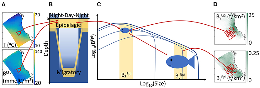
Figure 1. Schematic of APECOSM. (A) Illustration of the 3D environmental forcing from simulations with the physical-biogeochemical model ROMS-BEC, including temperature T and biomass of lower trophic levels (B^LTL). (B) The 3D environmental forcing defines the habitat of distinct epipelagic and migratory communities. (C) Environmental conditions influence individual metabolism at different sizes, modulating growth, feeding, reproduction, and mortality, thus driving the temporal evolution of the biomass density size-spectrum, here shown for epipelagic fish (B^Epi). (D) The integrated biomass of different size ranges determines the spatial biomass distribution, here shown for small ($B_S^{Epi}$) and large ($B_L^{Epi}$) fish. Neighboring cells (red squares) exchange biomass by passive transport and active swimming.

Temperature (T), biomass of lower trophic levels (B^LTL), dissolved oxygen concentration (O₂), and photosynthetically available radiation (PAR) determine the daytime and nighttime preferred habitats of communities along the water column (see Figures 1A,B). Thus, the epipelagic community remains near the surface all the time and includes forage species such as sardines and anchovies. The migratory community accounts for the nighttime surface migration of mesopelagic fish that follow their zooplankton prey at the surface. This migratory community also contains large diving predators such as tuna, billfish, and sharks that feed both on epipelagic and mesopelagic organisms (Glaser et al., 2015).

The temperature and food concentration determine the metabolism of individuals of each community (Figure 1C). Size-dependent growth, maturation, and reproduction are represented according to the Dynamic Energy Budget theory (DEB) with parameters derived from DEB models for fish (Kooijman and Lika, 2014). Small individuals feed on lower trophic levels, B^LTL, while larger individuals feed on smaller prey. All rates vary with temperature following the Arrhenius equation. By integrating individual-level responses for species of different asymptotic size (Lm), APECOSM calculates the biomass density distribution of each species, i.e., the biomass per unit volume per unit size (L). Summing biomass density distributions for all species with Lm between 1 mm and 2 m (here discretized by 6 species with Lm = 0.1, 0.3, 0.6, 0.9, 1.4, and 2 m), the model simulates the community size-spectrum (see Figure 1C showing the biomass density distribution $B_{sim}^{Epi}$ for the epipelagic group as example). Note that this specific discretization is an approximation of the model equations to account for biodiversity. All fish species of asymptotic size between 1 cm and 2 m are represented, from forage fish species to large sharks or tunas. Since larger individuals feed on smaller ones, different communities interact via predation when they co-occur in the water column. As shown in Figure 1B, epipelagic and migratory fish co-occur during the night at the surface. Accordingly, fish feed within their communities separately during the day, and on both communities during the night.

Integrating the community size-spectra enables the calculation of the total biomass for different size ranges. Here, for diagnostic purposes, we subdivide the size spectrum into small (S, 0.03 < L < 0.3 m), medium (M, 0.3 < L < 0.9 m) and large (L, 0.9 < L < 2 m) size classes. In the following, the biomass density of small epipelagic organisms will be indicated by $B_S^{Epi}$, of medium epipelagic fish by $B_M^{Epi}$, etc. (see Figures 1C,D). Environmental properties and feeding interactions ultimately determine the biomass density distributions at each grid point (Figure 1D). Beyond biomass density, the local computation of biomass accumulation due to growing individuals or recruitment, along with biomass losses due to mortality terms, allows the identification of regional sources and sinks of biomass.

The model accounts for movement by explicitly resolving passive advection by currents (with velocity $\overrightarrow{V}$), and active swimming between neighboring grid cells (Figure 1D, the red squares). Swimming is modeled as a size-dependent advection-diffusion process that represents the migration of fish toward more favorable habitats (Faugeras and Maury, 2007). Movement influences sources and sinks by spreading biomass of passively advected organisms and aggregating actively swimming predators.

2.1.2. Physical and Biogeochemical Forcing

We force APECOSM-CC with a realistic three-dimensional (3D) ocean model simulation of the California Current based on the Regional Oceanic Model System (ROMS, Shchepetkin and McWilliams, 2005) coupled online with the Biogeochemical Elemental Cycling model (BEC, Moore et al., 2004). This ROMS-BEC simulation has been run for the period 1997-2007 at a horizontal resolution of 4 km (i.e., mesoscale eddy-resolving) that reproduces accurately the main patterns of physical and biogeochemical variability in the region (Deutsch et al., 2021; Renault et al., 2021). Daily ROMS-BEC outputs on a coarsened grid (resolution of 16 km) are used to drive the food web dynamics (daily) and biomass transport (72 steps per day) in APECOSM-CC. Physical forcings consist of temperature (T) and current velocities ($\overrightarrow{V}$). Biogeochemical forcings consist of dissolved oxygen (O₂), PAR, and the biomass of lower trophic levels B^LTL that includes diatoms (B^Diat), zoo-plankton (B^Zoo), and particulate organic carbon (B^POC) computed from particle flux F_POC divided by a representative sinking velocity of 20m/d.

2.1.3. Parameters and Uncertainty

APECOSM-CC models pelagic fish in the California Current and relies on a total of 48 parameters and constants (see Table 1 and Supplementary Information 1). Many of these parameters are well-constrained by the literature, while other remain to be specified. Among them, five parameters describe predator-prey interactions, and six control coupling with ROMS-BEC (see Table 1). We determine them by testing the sensitivity of simulations on predetermined parameter ranges and choosing the values that produce the best match to observations (Section 3.1.2).

TABLE 1

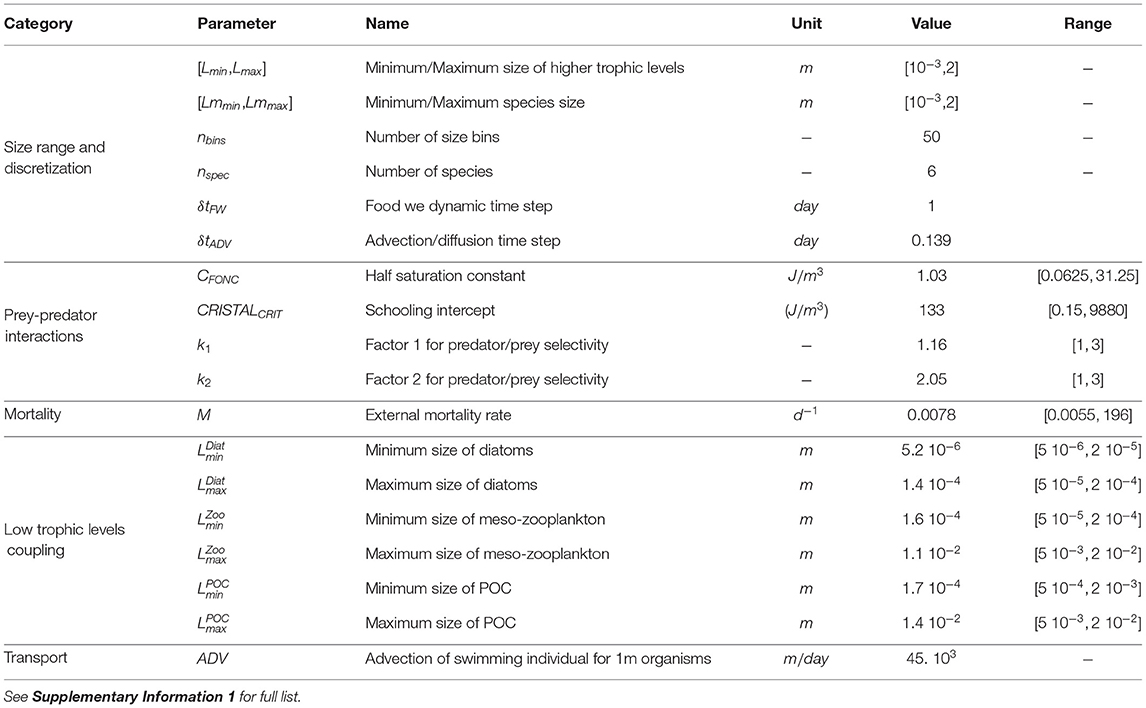
Table 1. Parameters in APECOSM-CC referenced in the main text.

First, predator-prey interactions depend on the rates of prey encounter and handling by predators. The half saturation constant (C_FONC) and schooling threshold (CRISTAL_CRIT) set the intensity of these interactions. The half saturation constant represents the limitation of biomass ingestion by encounter or assimilation rates, and falls within the range [0.0625, 31.25] J/m³ (see Supplementary Information 2). The schooling threshold determines the relative biomass density above which 50% of prey become accessible to predation, the remaining 50% assumed to be too dispersed to be effectively preyed upon (Maury, 2017). Based on the minimum and maximum biomass densities of lower trophic levels (B^LTL) we select it within the range [0.15, 9880] J/m³ (see Supplementary Information 3).

Second, feeding follows a selectivity function that depends on the predator-prey mass ratio (PPMR) and selectivity width (σ). In APECOSM-CC, both parameters are controlled by two constants, k₁ and k₂, that we set to be within the range [1, 3], leading to a predator-prey mass ratio within [245, 19260] for a 0.25 m long predator, and a selectivity width within [1.0, 1.7] (see Supplementary Information 4 for details).

Third, the model accounts for predation mortality, aging, and starvation. A density-dependent background mortality is included to account for external sources of mortality (M), including disease, predation by functional groups not explicitly represented by the model, and fishing mortality. To determine this background mortality, we assumed that if there were no predation from the simulated spectrum, no aging, no starvation, and no biomass production due to growth, the biomass of the smallest individuals would disappear over a timescale ranging from 1 week to 6 months. This loss corresponds to a background mortality rate within the range of [0.0055, 196] d⁻¹ (see Supplementary Information 5).

Finally, the size range of lower tropic levels provided by ROMS-BEC influences the coupling with APECOSM-CC since this size range controls the fraction of lower trophic level biomass accessible to upper trophic levels. In other words, for the same biomass density at low trophic levels, larger sizes of prey will be accessible to larger predators, depending on their prey selectivity range (see Supplementary Information 6), thus affecting energy transfer up the food web. The prey size range is controlled by 6 configuration parameters that determine the smallest and largest diatom cells, zooplankton organisms, and POC ($L_{min}^{Diat,Zoo,POC}$, $L_{max}^{Diat,Zoo,POC}$). We allow slight variations of these minimum and maximum sizes around default values, 10 − 100μm for the diatoms, 100 − 10, 000μm for the zoo-plankton, and 1, 000 − 10, 000μm for particles (see Table 1).

2.2. Pelagic Fish in the California Current

2.2.1. Surface- and Mid-Water Trawls

To tune and evaluate APECOSM-CC, we used data from ~1, 700 fisheries independent trawls collected by several surveys extending from the epipelagic to the mesopelagic zones: Coastal Pelagic Species (CPS) surveys conducted by the NOAA Southwest Fisheries Science Center (SWFSC); R/V Melville cruise P0810 of the California Current Ecosystem LTER program (CCELTER); R/V New Horizon survey for the Scripps Environmental Accumulation of Plastic Expedition (SEAPLEX); and the R/V McArthur II survey Oregon California and Washington Line-transect and Ecosystem (ORCAWALE) conducted by SWFSC.

The Surface-Water (SW) CPS surveys (Zwolinski et al., 2014) provide 1, 556 distinct trawl-based biomass estimates from March to October between 2003 and 2016 (Figure 2A, data available at ERDDAP, 2019). Most of these surveys consist of nighttime surface trawls, targeting fish aggregations with Nordic 264 trawls, covering most of the California Current, with higher occurrence nearshore (Figure 2B). We use the surface-water trawls to estimate the observed biomass density distribution of epipelagic species $B_{obs}^{Epi}$ in the size range [0.03, 2.]m (see Supplementary Information 7 for the conversion of trawls into biomass densities). Surface-water trawls also provide species composition for each trawl. Combining the weight per species sampled (w_s) and the species asymptotic sizes (Lm_s) from Fishbase (Froese and Pauly, 2016), we estimate the mean asymptotic fish length for each trawl (${\overline{Lm}}_{obs}=\sum L{m}_s{w}_s/\sum w_s$). We compute ${\overline{Lm}}_{obs}^{Epi}$ for pelagic species with a depth range shallower than 150 m (based on Fishbase); ${\overline{Lm}}_{obs}^{Meso+Mig}$ for vertically migrating species, i.e., migratory pelagic fish with a depth range deeper than 150 m, and mesopelagic fish (see Section 3.2.1). Finally, for a fraction of the surface-water trawls the length of each individual (L) is also measured. We use these to determine the abundance of individuals of different size in logarithmically equal bins and compare this distribution, the size spectrum, with simulations (see Section 3.2.2 and Supplementary Information 7 for more details).

FIGURE 2

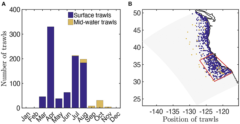
Figure 2. Trawl data in the California Current. (A) Total number of fisheries independent trawls per month. (B) Spatial distribution of fisheries independent trawls (blue, surface trawls; orange, mid-water trawls) and focus region for fish biomass time-series reconstruction (red).

In addition, Mid-Water (MW) trawls from the SEAPLEX, ORCAWALE, and CCELTER cruises from August to November in 2008 and 2009, are used to estimate the biomass density distribution in deep waters (Figure 2A, data provided in Davison et al., 2013). These trawls are conducted during the day and at night, down to different depths, with Isaacs-Kid trawls (IKMT, Orca-Wale, 95 trawls) or Matsuda-Oozeki-Hu trawls (MOHT, Seaplex, and CCE, 55 trawls) and target centimeter-size forage and mesopelagic fish. The trawls cover the entire California Current, from coastal to offshore waters (Figure 2B). We use the mid-water trawls to estimate the observed biomass density distribution of vertically migrating species $B_{obs}^{Mig}$ in the size range [0.0017, 0.1] m (see Davison et al., 2013 for the biomass estimates).

To complement the trawl observations, we use the biomass reconstruction by Koslow and Davison (2016) of the spawning stock biomass for epipelagic and mesopelagic planktivores from 1951 to 2011 in the Southern California Current (see region in Figure 2B). We use these reconstructions to obtain estimates of the average, minimum, and maximum ratio of epipelagic to migratory mesopelagic biomass over this period, resulting in $\overline{B_{obs}^{Mig}/B_{obs}^{Epi}}=7.53$, $max(B_{obs}^{Mig}/B_{obs}^{Epi})=20.7$, and $min(B_{obs}^{Mig}/B_{obs}^{Epi})$ = 2.38, respectively.

2.2.2. Species Occurrence and Asymptotic Lengths

Occurrence data obtained from the Ocean Biodiversity Information System database (OBIS, 2020) are used to inform the spatial distribution of species of increasing size in the California Current. We compiled spatial occurrence along with life-stage and species identity for surface epipelagic fish, vertically migrating predators, and mesopelagic fish, respectively, accounting for $n_{obs}^{Epi}=4,088$, $n_{obs}^{Mig}=10,279$ and $n_{obs}^{Meso}=11,638$ occurrences each. From the species identity, we associated each occurrence to the species asymptotic size (Lm, using Fishbase, Froese and Pauly, 2016) and determined the proportion of small (0.04 < Lm < 0.4 m), medium (0.4 < Lm < 0.9 m), and large (0.9 < Lm < 2 m) species as a function of the distance d from the coast, calculated along regular bins of width dx = 33 km. This cross-shelf probability of occurrence of species of increasing asymptotic size provides an observational estimate of the distribution of different sizes classes in the California Current (see Section 3.3.1 and Supplementary Information 8).

2.3. Simulation and Analysis

2.3.1. Implementation and Uncertainty

To constrain the 11 undetermined model parameters that control predator-prey interactions, background mortality, and coupling of APECOSM with ROMS-BEC, we develop a calibration procedure on a simplified one-dimensional (1D) configuration of the domain, here referred to as APECOSM-1D. The model reduces spatial variability to 15 independent 1D stations representative of 15 eco-regions in the California Current (see Figure 3A and Supplementary Information 9). At each station, we drive APECOSM-1D with environmental forcings based on simulated year 2001 from ROMS-BEC, averaged over the eco-region (Figure 3B). Each station is spun-up for 100 years to reach a stable seasonal cycle, and is then analyzed. The model timestep for predatory interactions, growth, and mortality is 1 day, averaging daytime and nighttime conditions. This simplified configuration disregards the role of horizontal movement, but reducing computational cost allows multiple simulations to select parameter combinations producing plausible regional variations of biomass density. We run 5, 000 replicates of this APECOSM-1D configuration applying a Monte Carlo approach, each with a distinct combinations of the 11 undetermined parameters randomly chosen from prior uniform distributions (see Figure 3C and Table 1 for the bounds of the distributions). This calibration further allows estimation of the sensitivity of the model to these undetermined parameters.

FIGURE 3

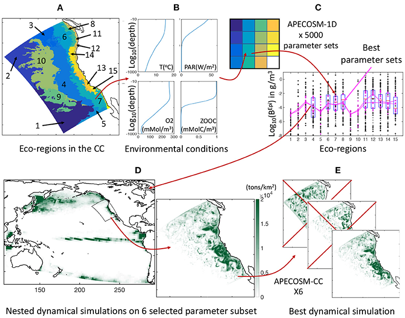
Figure 3. Schematic of the optimization approach. (A) Eco-regions of the California Current used as independent stations for model tuning. (B) Illustration of averaged vertical profiles used to force the model in each station, here station #7. (C) Illustration of the Monte Carlo procedure, whereby each eco-region is reduced to a single grid cell in APECOSM-1D, 5, 000 replicates of this 1D configuration are run, and optimal parameter sets are selected by comparison with observations. (D) Illustration of the parent Pacific and nested California Current 3D dynamical simulations. (E) Selection of the best regional 3D dynamical simulation from six optimal simulations with different parameter sets.

By comparing the ensemble of APECOSM-1D simulations to observations, we identified 6 best plausible parameter sets (see Section 3.1.1). With these we run six replicates of the 3D APECOSM-CC model forced with dynamic output from ROMS-BEC. Fish, especially large predators such as tuna, billfish, and shark species, often travel large distances as part of migration patterns (Block et al., 2011). In the model, large predators could periodically move inside and outside of the simulation domain. To account for this biomass transport, our California Current configuration is “nested” within a “parent” APECOSM simulation for the Pacific Ocean. This simulation was run for a repeated climatological annual cycle, at 64 km resolution, forced by a Pacific ROMS-BEC configuration with similar parameterization as the configuration of the California Current (see Figure 3D), following established approaches (Lemarié et al., 2012; Deutsch et al., 2021). Daily fish biomass predictions from the parent APECOSM are nudged at the boundaries of the regional configuration for incoming biomass fluxes, while outgoing biomass fluxes leave the domain. A two-dimensional boundary radiation scheme is used to estimate these fluxes (Marchesiello et al., 2001). These nested simulations are span-up with repeated 2001 annual forcing for 100 years and resolve spatial transport with a timestep of 20 min for numerical stability (72 steps per day).

To analyze the role of transport in structuring marine ecosystems, we keep the 3D simulation that best reproduces biomass densities in eco-regions (see Figure 3E), and then force it with dynamic outputs from ROMS-BEC on two inter-annual cycles of 10 years (1997 to 2006). We analyze the last 8 years from weekly outputs. To account for the uncertainty introduced by undetermined model parameters in this simulation, we run 10 replicates with slight parameter variations, ±10% for food web parameters, and ×3 or ×1/3 for movement parameters.

2.3.2. Diagnostic Features of Fish Communities

At each grid cell, APECOSM calculates the biomass density ${\xi }_{L,Lm}^{Epi,Mig}$ per size class L, per species asymptotic size Lm, for the epipelagic and migratory communities. For comparison with observation and analysis, we sum biomass over various combinations: $B_{S,M,L}^{Epi,Mig}$ the biomass of small, medium, and large fish; $B_{SW}^{Epi,Mig}$ and $B_{MW}^{Epi,Mig}$ the biomass over size ranges, respectively matching surface- and mid-water trawls selectivities; B^{Epi, Mig} the total biomass density per community (see Table 2 for the equations). To address the cross-shore structuring of the California Current (Ruzicka et al., 2016; Messié and Chavez, 2017), we also characterize the relative distribution of small, medium, and large fish groups by analyzing biomass along a cross-shore section. This cross-shore distribution is estimated by averaging the biomass density $B_{S,M,L}^{Epi,Mig}$ in regular spatial distance bins i (dx_i = 33 km) from the coast to the open ocean. Furthermore, for sensitivity analysis the “spread” of the biomass distribution in the region is summarized by the distance from coast ($d_{S,M,L}^{50\%}$) within which 50% of the total biomass in the region (${\text{B}}_{S,M,L}^{Epi,Mig}$) occurs (see Table 2).

TABLE 2

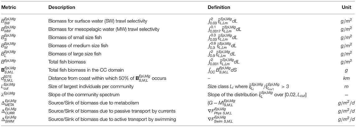
Table 2. Metrics for the analysis of ecosystem features.

The size of the largest individuals sustained in each community is an emergent property of the model (Guiet et al., 2016a). We compute the maximum length reached in each numerical cell, $L_{cut}^{Epi,Mig}$, for the epipelagic and migratory communities, as the size at which the community-level biomass density distribution ${\tilde{\xi }}_L^{Epi,Mig}$ “breaks,” i.e., the size above which biomass rapidly drops (see Table 2). Because the community-level biomass size spectrum roughly follows a power law, we use the power law slope λ^{Epi, Mig} between the minimum (L = 2 cm) and maximum size (L_cut) as a metric of the relative abundance of small and large individuals.

Finally, the model allows analyzing the mechanisms that lead to local biomass accumulation or reduction and how these relate to spatial transport. We extract net sources and sinks of biomass in each grid cell, as driven by the following processes: local growth and mortality (${\Delta }_{META}^{Epi,Mig}$); transport by currents (${\Delta }_{CURR}^{Epi,Mig}$); transport by swimming (${\Delta }_{SWIM}^{Epi,Mig}$) (see Table 2 and Supplementary Information 10 for the growth G, mortality M, and biomass fluxes F_Phys,Swim). Their cross-shore distribution is estimated like for the biomass.

3. Results

3.1. Biomass Distribution in the California Current

3.1.1. Selection of a Best Simulation

The 5,000 simulations with APECOSM-1D lead to a variation of several orders of magnitude for epipelagic ($\overline{B_{MW}^{Epi}}$) and migratory ($\overline{B_{MW}^{Mig}}$) biomass, once averaged over the 15 eco-regions (see Figure 4B). Only 16% reproduce the observed biomass density from mid-water trawls, $\overline{B_{MW}^{Mig}}=17g/m^2$, ±1 order of magnitude (horizontal lines Figure 4B). The ±1 order of magnitude range corresponds to the observed variation between the less productive offshore trawls and the trawls in the coastal upwelling (see observations Figure 5). It allows the selection of parameter sets over- or under-estimating the migratory biomass density that might be corrected once explicit spatial transport is included. A smaller fraction (3%) also capture the observed ratio of mesopelagic to epipelagic biomass, namely $2.38<\overline{B_{MW}^{Mig}}/\overline{B_{MW}^{Epi}}<20.7$ (oblique lines Figure 4B, see Supplementary Information 11 for the sensitivity of APECOSM-1D).

FIGURE 4

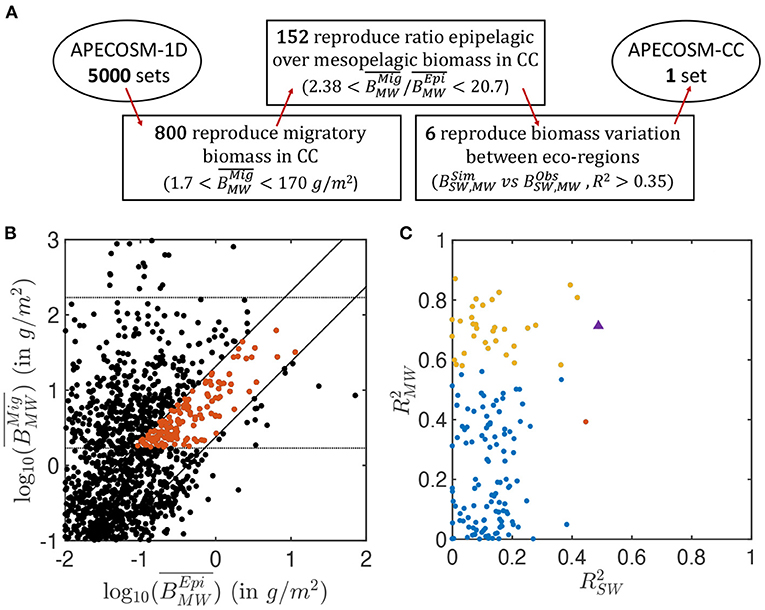
Figure 4. Summary of the ensemble of simulations with APECOSM-1D. (A) Schematic of the steps used to identify the optimal parameter sets. (B) Average migratory biomass density ($\overline{B_{MW}^{Mig}}$) as a function of average epipelagic biomass density ($\overline{B_{MW}^{Epi}}$). (C) Coefficient of determination of the correlation between observed and simulated $B_{SW}^{Epi}$, $B_{MW}^{Mig}$, in the 15 eco-regions, for the best ensembles shown in red in (B). In (B), the dotted horizontal lines show the acceptable range for migratory biomass densities. The solid diagonal lines show the limits of acceptable migratory to epipelagic biomass ratio based on observations (between 2.38 and 20.7). In (C), the red and yellow dots corresponds to ensembles for which epipelagic and mesopelagic biomass respectively correlate significantly with observations (p < 0.05) (note that there is only one red dot). Blue dots are ensembles for which there is no statistically significant correlation between simulations and observation. The purple triangle corresponds to the final best set of parameters selected for the 3D APECOSM-CC dynamic simulations.

FIGURE 5

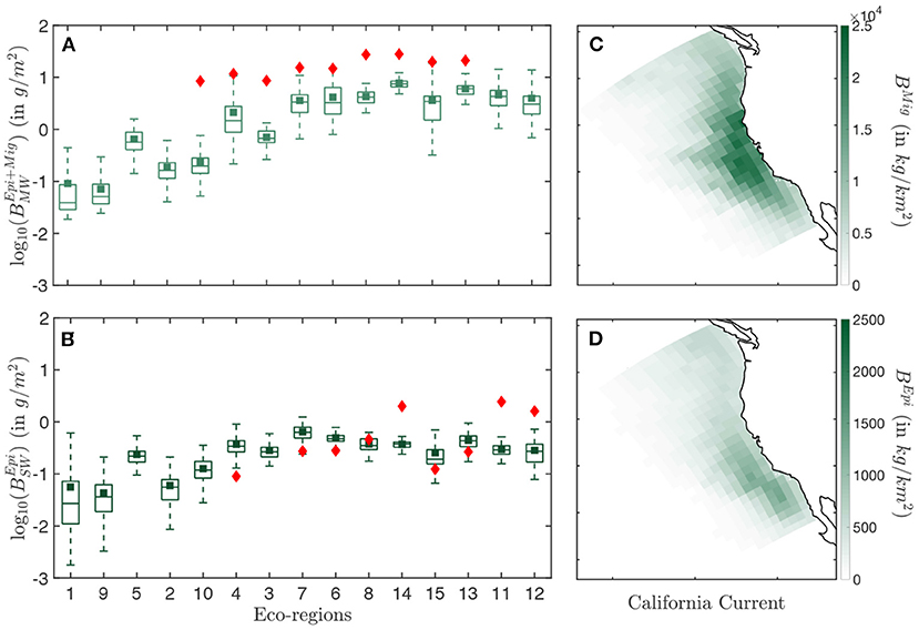
Figure 5. Biomass distribution in the California Current. (A) Simulated (light green) and observed (red) biomass densities B^Epi+Mig per eco-regions for the mid water (MW) trawls. (B) Simulated (dark green) and observed (red) biomass densities B^Epi per eco-regions for the surface water (SW) trawls. (C) Spatial distribution of the annual mean biomass density for the migratory community B^Mig binned in Δx = 96km grid cells. (D) Spatial distribution of the annual mean biomass density for the epipelagic community B^Mig, binned in Δx = 96 km grid cells. The simulation results in (A,B) are determined from the average of years 1999–2006. Eco-regions are ranked from low to high primary production. In the box-plot the central mark indicates the median, the bottom, and top edges of the box indicate the 25th and 75th percentiles, respectively, while the whiskers extend to the most extreme data points that are not considered to be outliers. The square marker is the averaged biomass density per eco-region, and the diamond the averaged observed biomass density per eco-region.

Out of these 152 simulations (shown in red in Figure 4B), an even smaller fraction captures the biomass variation between different eco-regions separately simulated by the 15 independent 1D stations. Figure 4C shows the Pearson correlation of annual mean simulated biomass densities in each of the 15 stations compared to mean observations for the epipelagic (compared with surface-water trawls) and migratory communities (compared with mid-water trawls) in the matching eco-regions (see Supplementary Information 9). Analysis of these correlations shows that different parameter sets can properly capture variations in epipelagic (red markers in Figure 4C, p < 0.05), migratory (yellow markers, p < 0.05), or both communities (purple marker) at statistically significant levels. We select 6 sets of parameters with higher coefficient of determination for both the epipelagic and migratory biomass densities ($R_{SW/MW}^2>0.35$) for fully dynamical simulations with APECOSM-CC (see Supplementary Information 11 for the parameters).

For these 3D simulations forced with dynamic ROMS-BEC output on a 16 km grid and that represent spatial active and passive transport, three out of six simulations maintain a realistic ratio between epipelagic and migratory biomass. We keep the simulation that best reproduces the regional biomass density gradients observed between eco-regions in the California Current (triangle marker in Figure 4; see Table 1 for best parameters; see Supplementary Information 12 for 6 APECOSM-CC simulations).

3.1.2. Observed vs. Simulated Biomass Distribution

Observation show an increase in biomass density in both the surface (SW) and mid-water (MW) layers when moving from less productive offshore waters (Figures 5A,B, red diamonds in eco-regions #3, 4, 6, 7, 10) to more productive coastal waters (#8, 11, 12, 13, 14, 15). Furthermore, seasonal eco-regions at higher latitudes (#6, 8, 11, 12, 14) hold comparatively higher biomass densities than more equatorward eco-regions (#7, 13, 15).

The spatial distribution of simulated biomass density corresponding to mid-water trawls ($B_{MW}^{Epi+Mig}$), when averaged from August to November to match the months of the observations (cf Figure 2A), reproduces observed patterns (R² = 0.76 for the correlation between model and observations, see Figure 5A). However, the model underestimates observations (green squares Figure 5A), with modeled biomass densities on average 29% lower than mid-water trawls. Spatially, the biomass density of vertically migrating fish B^Mig is higher on the shelf and in the core of the upwelling, and much smaller offshore (Figure 5C).

For surface-water trawls, when averaged from March to August to match observation (cf Figure 2A), regional variations of simulated biomass densities for epipelagic fish are poorly captured (R² = 0.07). This weak correlation mostly originates from a strong underestimate of the biomass density $B_{SW}^{Epi}$ in the coastal regions (#11, 12, 14 Figure 5B). Away from the coast, regional averages match more closely the surface-water trawls. Similar to migratory biomass, epipelagic biomass also accumulates along the coast, but is higher toward the southern limb of the upwelling and the Southern California Bight (Figure 5D).

Overall, dynamic simulation leads to a coherent distribution of migratory biomass, and a more irregular distribution of pelagic biomass. In the southern California Current (red box in Figure 2), the average ratio of pelagic to migratory biomass is well within the range of observations, i.e., $\overline{B_{MW}^{Mig}}/\overline{B_{MW}^{Epi}}=10.68$.

3.1.3. Sensitivity to Parameters Uncertainty

A parameter sensitivity analysis with the best simulation indicates that the predation parameters k_1,2 exert the strongest controls on biomass accumulation $\overline{{\text{B}}^{Epi+Mig}}$ (Figure 6). Larger predator-prey mass ratio (k₁ − 10% or k₂ + 10%) increase biomass accumulation in the domain. This accumulation benefits the migratory community, such that $\overline{{\text{B}}^{Epi}}/\overline{{\text{B}}^{Mig}}$ decreases. The latter also reaches smaller size $\overline{L_{cut}^{Mig}}$. Thus, the biomass of larger individuals decreases to the benefit of smaller ones (see variations of $\overline{{\text{B}}_{S,M,L}^{Epi,Mig}}$). Opposite responses are observed for smaller predators-prey mass ratios (k₁ + 10% or k₂ − 10%). The cross-shore biomass distribution is slightly impacted by variations of the predation parameters (see changes in $d_{S,M,L}^{50\%}$).

FIGURE 6

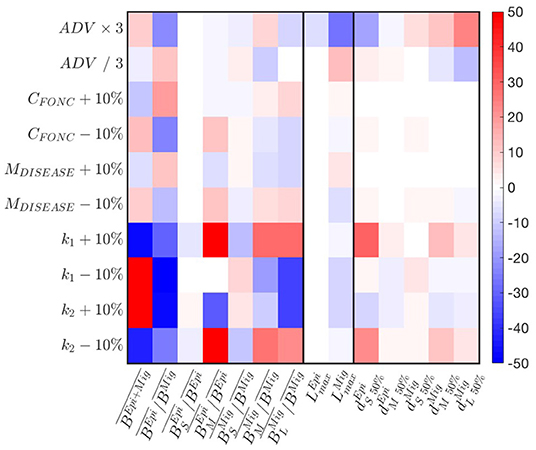
Figure 6. Sensitivity of APECOSM-CC to food-web parameters. We test variations around ±10% for the food-web parameters, × / 3 for the parameters controlling movement. The sensitivity is expressed as % variation compared to the reference simulation with the best parameter set.

A decrease of prey searching rate, obtained by increasing the half saturation constant C_FONC, and the increase of mortality M, both decrease biomass accumulation, while benefiting epipelagic fish, such that $\overline{{\text{B}}^{Epi}}/\overline{{\text{B}}^{Mig}}$ increases. While the effects translate to variations of the relative abundance of small, medium and large fish (see $\overline{{\text{B}}_{S,M,L}^{Epi,Mig}}$), they have almost no impacts on the spatial biomass distribution (see $d_{S,M,L}^{50\%}$). Opposite responses are observed for increasing searching rate C_FONC and decreasing M.

Finally, a faster swimming speed (ADV) allows increasingly large migratory fish to expand their distribution offshore, while epipelagic fish tend to cluster nearshore (see changes in $d_{S,M,L}^{50\%}$ in Figure 6). This drives an accumulation of biomass that benefits epipelagic species, such that $\overline{{\text{B}}^{Epi}}/\overline{{\text{B}}^{Mig}}$ increases, while the maximum size of migratory species $\overline{L_{cut}^{Mig}}$ decreases.

Sensitivity tests shown in Figure 6 reveal that most features of a fully dynamical simulation are similarly or less impacted than the amplitude of variation applied to a single parameter, suggesting non-linear, compensatory effects in the model. Except for the predator-prey selectivity parameters k_1,2, most variations are within the ± 10% or 1/3 to 3 × range. Thus, fully dynamical simulations and the following analysis are robust to small parameter variations.

3.2. Emergent Features of Fish Communities

3.2.1. Community Maximum Sizes

The average fish size from trawl observations (${\overline{Lm}}_{obs}$) is different for epipelagic and migratory species (Figure 7 and Supplementary Information 7). Epipelagic species are mostly smaller, with asymptotic sizes between 0.165 and 3.3 m, and a mean of 0.4 m (Figure 7A in blue, note that distributions are displayed on a logarithmic scale). Migratory species exhibit a larger range, from 0.077 to 4 m, with two modes, the first around 0.2 m when migratory mesopelagic fish dominate the trawls, and the second around 1 m when large predators are captured (Figure 7B in purple).

FIGURE 7

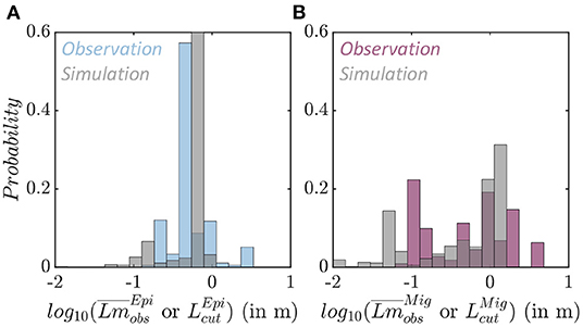
Figure 7. Species size distributions. (A) Observed average species size per trawl ${\overline{Lm}}_{obs}^{Epi}$ (blue) and simulated maximum size per grid cell (gray) for the epipelagic community $L_{cut}^{Epi}$. (B) Observed average species size per trawl ${\overline{Lm}}_{obs}^{Mig}$ (purple) and simulated maximum size per grid cell (gray) for the migratory community $L_{cut}^{Mig}$.

In APECOSM-CC, the environment determines the maximum size of the species sustained in each grid-cell for each community. The maximum size per community ($L_{cut}^{Epi,Mig}$) simulated in each grid cell of the domain matches observed size differences. Epipelagic species are smaller, with a mean maximum size of 0.62 m (Figure 7A in gray). Migratory species reach larger sizes, up to 1.3 m at most locations (Figure 7B in gray). The sensitivity analysis shown in Figure 6 indicates that this maximum size is sensitive to the predator-prey selectivity range (k_1,2), as well as parameters controlling swimming (ADV).

3.2.2. Size-Spectra Slopes

In the simulations, the biomass density distribution closely follows a power law (see the average size spectra in Figure 8A). Regional variations in the power law slope (λ) reveal variations of the biomass of large individuals relative to small ones. Note that here slopes are expressed as a function of fish weight or volume, derived from size following V = (δL)³, with δ a shape factor (see Supplementary Information 1).

FIGURE 8

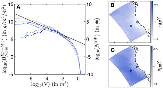
Figure 8. Biomass size spectra. (A) Envelop for the simulated normalized biomass size-spectra (dotted line) and observed biomass size-spectra (solid line), in a coastal (light blue) and an offshore (dark blue) cell. (B) Slopes λ^Epi of the local average size-spectra for the epipelagic community. (C) Slopes λ^Mig of the local average size-spectra for the migratory community. In (A), the black line shows the expected theoretical slope of λ = −1. In (B,C), the light/dark blue dots indicate the cells where coastal/offshore biomass spectra (A) come from.

For the epipelagic community, λ^Epi is steeper close to the shore, and shallower offshore (see Figure 8B). As the slope becomes less steep, the biomass of small fish decreases compared to the biomass of large individuals (see simulated spectra Figure 8A). This relative decrease of small fish biomass in coastal relative to offshore waters agrees with observations, where fewer small individuals are found in surface trawls moving from the coast to the open ocean (solid lines in Figure 8A). Note that observed size spectra break for sizes smaller than V = 10⁻⁴ m³. In this range, a systematic decrease in biomass abundance can be in part attributed to a decreasing selectivity of sampling gear to small individual sizes.

For the migratory community, simulated spectral slopes show a similar trend (see Figure 8C), with generally shallower values. Thus, larger predators are relatively more abundant among vertically migrating fish species, as supported by the larger sizes reached by this community (see Figure 7).

3.3. Cross-Shore Biomass Distributions

3.3.1. A Cross-Shore Size Succession

Biomass size-spectra indicate a cross-shore variation of the relative abundance of larger and smaller fish in the California Current (Figure 8). Figures 9A,B highlights this variation for small, medium, and large individuals along an average cross-shore section. For the epipelagic community, only small (0.03 < L < 0.3 m) and medium-size (0.3 < L < 0.9 m) fish survive in the domain (see species size distribution in Figure 7A). Most small fish are found near the coast (Figure 9A, $d_S^{50\%}=229$ km), while medium-size fish are spread farther offshore ($d_M^{50\%}=357$ km). For the migratory community, in addition to small- and medium-size individuals, large predators (0.9 < L < 2 m) survive. A similar pattern of increasingly spread-out biomass from small to large fish is also observed for this community (Figure 9B, $d_S^{50\%}=200$ km, $d_M^{50\%}=294$ km, $d_L^{50\%}=425$ km).

FIGURE 9

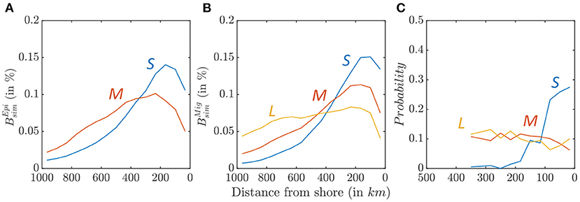
Figure 9. Biomass density along a cross-shore section, for small (blue), medium (red), and large size (yellow) fish. (A) Relative distribution of simulated epipelagic biomass distribution $B_{sim}^{Epi}$. (B) Relative distribution of simulated migratory biomass distribution $B_{sim}^{Mig}$. (C) Observed relative distribution from OBIS species occurrence data.

This cross-shore spread is comparable with the observed species distribution from the OBIS database (Figure 9C, when all sample are considered, see Supplementary Information 8 for additional details). While small species (0.04 < Lm < 0.4 m) cluster nearshore, medium (0.4 < Lm < 0.9 m), and large (0.9m < Lm) species are more homogeneously distributed. Simulations and observations cannot be directly compared, because the OBIS database reports presence but not abundance. However, these patterns suggests higher occurrence of small fish in coastal water, while large fish tend to occupy the entire ecosystem.

Sensitivity tests suggest that the biomass spread for distinct size groups is mostly sensitive to the swimming parameter (ADV), and the predator-prey selectivity parameters (k_1,2; Figure 6). For ADV, an increased swimming capability leads to offshore spread of migratory species, and vice versa. For k_1,2, smaller predator-prey size ratios lead to a relative increase of biomass near the coast.

3.3.2. Drivers of Cross-Shore Succession

The best APECOSM-CC simulation is tuned to reproduce observed biomass densities. These densities are controlled by three main processes: (1) net or surplus production, modulated by environmental conditions; (2) current-driven redistribution from source to sink regions; (3) active swimming toward favorable conditions, i.e., from sink to source regions.

Figures 10A–C shows the difference between production and respiration (Δ_META) for the epipelagic and migratory communities. Positive surplus production is observed in productive nearshore waters for smaller individuals in both communities (primary production shown in Supplementary Information 13). Moving offshore, surplus production rapidly decreases from positive to negative values, becoming a sink of biomass when mortality exceeds new production (Figures 10A,B). Medium- and large-size species feeding on small fish tend to accumulate new biomass further offshore. This cross-shore gradient in production is slightly stronger for the epipelagic community. The enhanced production nearshore and dissipation offshore are consistent throughout the CC region, except along the southern coast where production nearly equals mortality, leading to limited surplus production (Figure 10C).

FIGURE 10

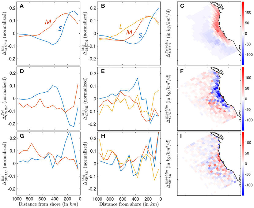
Figure 10. Biomass accumulation and dissipation along a cross-shore section, for small (blue), medium (red), and large (yellow) fish, reflecting food-web dynamics and spatial transport processes. (A–C) Surplus production for pelagic and migratory communities Δ_META. (D–F) Accumulation and dissipation due to passive advection by currents for pelagic and migratory communities Δ_CURR. (G–I) Accumulation and dissipation due to active swimming for pelagic and migratory communities Δ_SWIM. The maps show averages binned in Δx = 96km grid cells to smooth spatial variability caused by mesoscale eddies.

Currents act to redistribute biomass by advecting newly-produced biomass away from the coast, and accumulating it in a band between 300 and 800 km, as revealed by Δ_CURR (see Figures 10D–F). Most of this redistribution affects smaller individuals with limited swimming abilities, in both epipelagic and mesopelagic communities. As individuals grow larger, this transport is increasingly independent of the cross-shore distribution, and increasingly variable, suggesting an increasing interaction with mesoscale eddies, rather than continuous advection by the mean current (Figures 10D,E). Since the bulk of biomass is found in smaller individuals, surplus biomass generated along the coast is on average advected offshore where it is mostly dissipated (see Figures 10C,F).

In the model, swimming tends to counteract the effect of currents. Small forage fish in both communities swim on average toward the productive upwelling region, driving biomass accumulation along a band within 400 km of the coast (see Δ_SWIM, Figures 10G,H). Swimming maintains the biomass of medium-sized migratory organisms along a similar coastal band (red line Figure 10H), while larger migratory fish (yellow line Figure 10H) and medium-sized epipelagic fish (red line Figure 10G) tend to swim off-shore. To some extent, active movement against the mean current compensates the background transport offshore (compare the amplitude of passive advection Δ_CURR and active swimming Δ_SWIM, Figures 10F,I). However, active swimming also interacts with highly variable oceanic currents, such as eddies, fronts, and filaments, diverting biomass from the coast to local features (as suggested by the increased patchiness in Figure 10I).

In summary, while most new production is coastal, as individuals grow larger their main food source shifts offshore because of the transport by the mean surface current. Moreover, larger and larger individuals are increasingly attracted by local circulation features that divert them away from the most productive coastal regions. We argue that both effects contribute to explaining the cross-shore biomass distribution discussed in Section 3.3.1.

4. Discussion

4.1. Simulated Biomass Distribution

Our simulations reproduce observed relationships between fish biomass, and primary productivity, with higher biomass in high latitude and upwelling waters, and lower biomass in offshore oligotrophic waters. The migratory community dominated by small mesopelagic fish determines most of these gradients (Figure 5A), as in Davison et al. (2013). Surface biomass densities are more homogeneously distributed over the domain, although with variations consistent with observations (Figure 5B). However, the model underestimates the large biomass densities in the coastal eco-regions of the northern corner of the domain by up to a factor 10. This underestimation might be partly explained by the strong southern coastal current coming from the north boundary of the domain. This current could advect coastal fish biomass from outside the simulation domain, from the Gulf of Alaska, allowing more accumulation than is currently possible when nudging the boundaries from a coarse 64 km resolution parent simulation.

Observations of surface fish biomass density are also substantially more variable than model simulations. Surface-water trawl surveys are designed to monitor epipelagic forage fish stocks (Zwolinski et al., 2012), and therefore target biomass aggregations. These aggregations, which are shaped by fronts and other mesoscale features (Woodson and Litvin, 2015; McGillicuddy, 2016), are not resolved down to the level of schools by the model, which cannot resolve the scale (hundreds of meters to kilometers) at which many of these abundant forage species are preferentially found (Maury, 2017). Thus, the model should be considered a representation of smoother, large-scale average conditions. On the contrary, mid-water trawls sample a more diffuse and homogeneous deep-scattering layer, as shown by the spatial persistence of deep scattering layers in acoustic transects (Wall et al., 2016; Proud et al., 2018). This homogeneity might reduce spatial variability and explain the better match between model and observations.

The biomass density for migrating mesopelagic fish (2.8 gm⁻² on average) is also underestimated by the model compared to the mid-water trawls, but matches other large-scale estimates for the region (e.g., 3.6 gm⁻² in Lam and Pauly, 2005) and other regional estimates (e.g., 7.6 gm⁻² in Field et al., 2006). Mesopelagic fish observations are associated with uncertainties, including trawl net avoidance and limited selectivity (Kaartvedt et al., 2012). Some of these uncertainties are accounted for in the mid-water trawls data that we use in this study (Davison et al., 2013). While additional fine-tuning of the model could help resolving this mismatch (see Figure 6), we kept the optimal parameters for the final simulation to avoid generating other mismatches.

Finally, while the model underestimates mid-water trawl biomass, the ratio of pelagic to migratory biomass ($\overline{B_{MW}^{Mig}}/\overline{B_{MW}^{Epi}}=10.68$) agrees with reconstructions for the California Current (Koslow and Davison, 2016), and other global estimates (Irigoien et al., 2014). Furthermore, the model epipelagic biomass roughly matches observations, if we acknowledge the higher variability and patchiness of surface-water trawl data.

4.2. Parameter Selection

Although mechanistic models often rely on fewer undetermined parameters than empirical models, some of these parameters remain poorly constrained. For instance, no single set of parameters defines the encounter between predators and prey for all species in epipelagic and mesopelagic communities. Additionally, there are no firmly established estimates of the fraction of individuals that die from disease or pollution. Therefore, we conducted a sensitivity analysis to evaluate the importance of 11 of these relevant parameters for the model and their effect on fish biomass distribution.

For predator-prey interactions, the optimal value for C_FONC (see Table 1) indicates a specific volume clearance rate of 30.34 10⁶ per day (see Supplementary Information 2). We were not able to find measures for adult fish to confirm this number, but it is within the range measured from fish larvae and other lower trophic level organisms (Kiørboe, 2011). The parameter CRISTAL_CRIT controls the intensity of feeding interactions, but is harder to compare to the literature. Tuning of this parameter mostly affects the relative biomass of epipelagic and migratory communities (see Figure 6).

Parameters that determine the shape of the prey size selectivity (k_1,2) influence the predator-prey mass ratio PPMR and the ability of predators to feed on a wider range of prey sizes (σ). Here, the best values for k_1,2 (Table 1), correspond to a PPMR = 4861, and a selectivity width of approximately one order of magnitude (σ = 1.13, see also Supplementary Information 4). The estimated PPMR and the variability of the selectivity are well within the range of expected values (Barnes et al., 2010; Reum et al., 2019). Consistently with theories that suggest that PPMR and σ have a strong effect on trophic efficiency (Brown et al., 2004; Eddy et al., 2020), these parameters most affect the model solution, with longer food-webs (small PPMR) leading to more biomass accumulation (see Figure 6). Moreover, both parameters influence the maximum sizes reached by communities (refer to the impact of k_1,2 on $L_{cut}^{Mig}$ in Figure 6).

The external mortality includes mortality terms not explicitly accounted for in the model, such as disease, pollution, or fishing. It influences the total biomass accumulation, and the relative biomass of different size groups (Figure 6). In particular, external mortality triggers a trophic cascade: as mortality increases, the biomass of larger individuals drops, favoring accumulation of small individuals (see effect of M_DISEASE Figure 6). The optimum mortality value selected by calibration (see Table 1) represents a daily mortality at any size class L of 0.0078 d⁻¹ when at maximum schooling density. In other words, in the absence of any other mortality, the time-scale for the biomass to be lost at high biomass density is 4 months. This mortality represents an upper bound since it depends on the biomass density (Maury and Poggiale, 2013). More abundant size classes or regions will be exposed to external mortalities at a higher rate than more diffuse size classes or regions, assuming lower disease transmission or lower fishing pressure on dispersed resources. Note that this external mortality term can be considered a closure term that allows reproducing realistic biomass density distributions by representing non-resolved processes that remove biomass, for example fishing. The dynamic of fishing includes complex interactions between available catches and socio-economical drivers (Maury et al., 2017; Scherrer and Galbraith, 2020). Their representation is beyond the scope of the current analysis.

Beyond parameterization of processes, the numerical discretization of the size dimensions influences the results of the simulations. Because of computational limitations, we discretized biodiversity with 6 asymptotic sizes, favoring a more refined representation of larger species by selecting Lm from 10 cm upward. In the smallest size classes, this discretization contributes to the deviation of the biomass distribution from a linearly decreasing biomass spectrum (see Figure 8A). In our analysis, we focus on individuals larger than 3 cm to minimize the effects of the coarse discretization of small size classes.

Finally, the physiology modeled by the DEB model represents ectotherm organisms, especially fish, since the parameterization is based on fish DEB models (Kooijman and Lika, 2014). We assume that this formulation is applicable to other temperature-dependent organisms that grow from small eggs to larger organisms, e.g., invertebrates such as krill and squids. Still, other important predators in the California Current are not explicitly represented, especially mammals and seabirds (Santora et al., 2021). Their explicit representation would require a separate formulation of the DEB physiological model, for example to include homeotherm physiology. However, their effect on pelagic communities is implicitly included through the background mortality, a biomass loss term necessary for the model to reproduce observed biomass distributions.

4.3. Forcing With ROMS-BEC

The complexity of the lower trophic level models, in particular their resolution of different functional types and size classes, is a sensitive component for simulation of biomass at upper trophic levels (Kearney et al., 2021).

The biogeochemical model BEC provides a simplistic representation of such size diversity with a basic size structure (two phytoplankton groups and one zooplankton group). To couple APECOSM-CC with ROMS-BEC, we tested multiple possible sizes ranges for the lower trophic levels when calibrating the model. The coupling appears weakly sensitive to the size range of diatoms and particulate organic carbon, and only the size range of zooplankton was identified as significant (see Supplementary Information 11). The spatial distribution of these lower trophic levels might be more important, because it determines gradients in suitable habitats. For example, the cross-shore biomass distribution for small fish ($B_S^{Epi,Mig}$ in Figures 9A,B) closely matches the distribution of their food (Supplementary Information 13). Note that compared to observations from the MAREDAT database (Moriarty and O'Brien, 2013), ROMS-BEC simulations underestimate zooplankton biomass nearshore, and overestimate it offshore (see Kessouri et al., 2020 and Supplementary Information 13). We suggest that this bias in lower trophic levels is partly responsible for an excessive spread of fish biomass offshore in our simulations.

The limited diversity of functional types in BEC might also impact the biomass transfer to upper trophic levels and simulated biomass distributions. For instance, cold and warm ocean conditions favor euphausiids and gelatinous zooplankton respectively in the California Current, leading to changes in mid-trophic level organisms (Brodeur et al., 2019). Further developments will be required to account for these effects properly.

4.4. Emergent Features

On quantities averaged over 10 years of simulation, the model can capture a series of emergent properties of the observed biomass distribution in the California Current.

First, simulations show higher biomass of small migratory mesopelagic fish (see Figure 4A), consistent with observations (Davison et al., 2013; Irigoien et al., 2014; Koslow and Davison, 2016). Since in the model surface epipelagic and deep-diving migratory communities share the same parameterizations, this property emerges from differences in their habitat. We suggest that differences in temperature, and the resulting metabolic rates, are behind these patterns. Surface epipelagic fish experience comparatively warmer conditions throughout the day, while migratory organisms experience colder waters during the day when they reside in the mesopelagic zone. The analysis of the sensitivity of biomass size-spectrum models to warming shows that a faster increase of metabolism and respiration with warming, relative to the increase of biomass assimilation, leads to decreasing community level biomass in warmer conditions (Guiet et al., 2016a). Inversely in cooler habitats, biomass accumulates. The difference in the temperatures experienced by organisms at different depths might favor biomass accumulation in cooler deep-sea waters. Note that the resident mesopelagic community that does not migrate is not modeled here, unlike in other applications of APECOSM (Maury, 2010). When this resident mesopelagic community is included in the simulations, the model fails to represent realistic coexistence with the vertically migrating mesopelagic fish and migrating predators (i.e., simulated biomasses for both communities are unrealistic). Current modeling assumptions might explain this mismatch. For instance, the model does not allow ontogenetic transitions from epipelagic to deep mesopelagic habitats, which can characterize mesopelagic species (Lourenço et al., 2017). Another possibility is that we parameterize predator-prey interactions in the same way across the three communities (i.e., prey selectivity or searching rates), ignoring potential differences in feeding habits between migrating and resident mesopelagic fish (Bernal et al., 2015; Drazen and Sutton, 2017). In observations, the resident mesopelagic biomass accounts for a relatively small fraction of the total mesopelagic biomass, which is dominated by diel vertical migrators (Koslow and Davison, 2016). Yet, resident organisms could affect small migrating prey (e.g., by feeding on them), and might contribute to the feeding strategy of large migrating predators. The inclusion of this community will be explored in future studies.

Second, epipelagic fish tend to be smaller than migratory fish (see Figure 7). While observed and simulated representative sizes are not perfectly comparable, the model reproduces a clear size difference between surface and migratory communities that agrees with observations. We suggest that the higher migratory biomass and lower metabolism in deep waters allow the development of more trophic levels in the migrating community, ultimately supporting larger species and individuals (Guiet et al., 2016a). Note that the maximum size reached by migratory predators ($L_{cut}^{Mig}=1.5m$) is below the maximum size allowed by the model (2 m), while observations show the occurrence of larger species ($max(L{m}_{obs}^{Mig})>2$ m), such as swordfish or white sharks. Many large deep-diving predators develop thermoregulation apparatuses (Legendre and Davesne, 2020; Braun et al., 2021) that might increase feeding efficiency and assimilation in deep waters (Fritsches et al., 2005). These adaptations may contribute to the increased asymptotic size of migratory species, but are absent in the model. Moreover, in the model, large pelagic predators completing diel migrations spend half of the day at depth, half of the day at the surface. This pattern is applied to all migratory predators; however, some species adopt different behaviors, e.g., sub-daily vertical migrations with sporadic deep dives (Braun et al., 2021). Fine-tuning or new parameterizations could also help reduce this bias (see Figure 6).

Third, an ubiquitous feature of marine ecosystems is the regularity of the biomass density distribution, which follows a power-law as a function of individuals size, at least within selected size ranges (Brown et al., 2004; Hatton et al., 2021). For the biomass density as a function of the individual structural volume (V = (δL)³), the slope of this power-law is empirically and theoretically shown to be close to λ ≈ −1 (Brown et al., 2004; Rossberg, 2012; Sprules and Barth, 2015). APECOSM-CC reproduces this emergent slope, with $\overline{{\lambda }^{Epi+Mig}}=-0.94$, and regional variations and inter-community differences (see Figure 8). Simulated variations around this mean value are large, since slopes as steep as −1.57 for the epipelagic community in the core of the upwelling, and as shallow as −0.71 offshore for the migratory community are simulated. The model suggests comparatively more small individuals nearshore, and fewer offshore. We argue that this shift is due to biomass redistribution between source and sink regions. Note that fishing has been shown to impact the slope of fish size spectra (Shin and Cury, 2004), an effect not explicitly included in our simulations.

4.5. Cross-Shore Biomass Spread

The model reveals an increase in the cross-shore biomass spread for individuals of increasing size (see Figures 9A,B). The pattern is comparable to observations from the OBIS database (Figure 9C), showing that smaller species are sampled more frequently along the coast, while larger species are sampled more uniformly across the region. Importantly, this cross-shore pattern extends to higher trophic levels a succession already documented for phytoplankton and zooplankton (Keister et al., 2009; Messié and Chavez, 2017).

This cross-shore distribution emerges in the model from surplus biomass production for small organisms near the coast, where lower trophic levels are more abundant. This excess production, likely trapped in the surface Ekman layer and mesoscale features, is then advected offshore, as observed for zooplankton in the California Current (Keister et al., 2009). Small fish biomass accumulates while being transported offshore, in turn feeding increasingly large predators. This cross-shore transport matches other modeling studies that link fish production to the level of retention modulated by upwelling intensity (Steele and Ruzicka, 2011; Ruzicka et al., 2016). Unlike zooplankton, fish can swim toward more favorable conditions at speeds faster than mean ocean currents, and can actively contribute to this retention. Active swimming could thus generate offshore hotspots where the passively advected lower trophic levels would overlap with their predators, for example, in regions where passively advected euphausids accumulate (Santora et al., 2021). Thus, we would expect all organisms to remain in the core of the productive upwelling region, or more precisely to remain where passively advected organisms accumulate. However, in the model, intense mesoscale currents and eddies lead to patchy biomass distributions, with organisms clustering around mesoscale eddies seeded with coastal biomass. Increasingly large predators are attracted by these high-biomass “oases,” limiting their ability to migrate toward the productive coastal regions (Figures 10G,H). Increased biomass aggregations along eddies and fronts might further affect the productivity for the higher trophic levels (Woodson and Litvin, 2015).

These cross-shore patterns depend on parameters that control predator-prey interactions. Shorter food-webs (i.e., larger PPMR) lead to enhanced coupling with lower trophic levels, and a biomass distribution that increases more rapidly toward the coast (see $\overline{B^{Epi+Nig}}$ and d_50% for various values of k_1,2, Figure 6). We suggest that with a larger PPMR, the distribution of primary consumers matches more closely the higher primary production near the coast, so that secondary consumers will also cluster onshore following their prey. Note that in our simulations the biomass of smaller mid-trophic levels is distributed more broadly offshore than suggested by the OBIS database. As shown by Figure 9, small organisms dominate within 400 km from the coast (blue lines in Figures 9A,B) while in observation they dominate within 100 km from the coast (blue line in Figure 9C). This bias can be partly attributed to biases in lower trophic level biomass in ROMS-BEC (see comparison with MAREDAT data, Moriarty and O'Brien, 2013, in Supplementary Information 13).

Interannual variations of upwelling intensity influence the coupling between low trophic levels and productivity (Ware, 1992; Ruzicka et al., 2016; Messié and Chavez, 2017), modulating the migration patterns of top predators between nearshore and offshore waters (Fiechter et al., 2016). Our analysis focuses on averaged quantities from 1997 to 2006 to reveal the cross-shore biomass spread in this highly dynamic ecosystem. Further analysis should investigate this interannual dynamic and how upwelling intensity influences the distribution of forage fish and large predators. We leave this to future work.

4.6. Ecological Relevance

A variety of modeling approaches has been applied to study fish communities in the California Current System, from species distribution models (Fiechter et al., 2016; Brodie et al., 2018) to end-to-end ecosystem models (Field et al., 2006; Horne et al., 2010; Kaplan et al., 2019). This study presents a trait-based model that disregards species identity and simultaneously resolves bottom-up propagation of biomass through the ecosystem, ultimately controlled by primary production, top-down predation, and redistribution of organisms shaped by currents and active swimming. Reproducing emergent properties, it complements previous modeling efforts and provides new ecological insights into the dynamics of this pelagic ecosystem.

In the California Current, upwelling intensity influences fish productivity directly, by controlling nutrient supply and primary production. It also exerts a control on surface circulation and water retention, and thus nutrient recycling and accumulation of lower trophic level biomass (Steele and Ruzicka, 2011; Ruzicka et al., 2016). Our analysis supports the idea that cross-shore currents decouple productive coastal upwelling waters from offshore fish aggregations (Figure 10). By representing the swimming ability of small to medium-sized species, our study also suggests a biologically mediated retention that might counteract this decoupling and enhance productivity, consistent with the generation of hotspots where multiple trophic levels overlap (Santora et al., 2021). However, our analysis also suggests a dispersive role of mesoscale eddies that might prevent large predators from co-occurring in these hotspots.

Predicting the productivity and presence of species of economic or ecological value is a central goal of many marine ecosystem modeling efforts for this region (Politikos et al., 2018; Cimino et al., 2020; Muhling et al., 2020), especially to understand where species will occur at different life stages, for instance, and to design marine protected areas (Gilman et al., 2019). By linking top-predators to primary production and ocean dynamics, our model shows how large predators in offshore waters depend on biomass redistribution (Figure 10C) and mesoscale dynamics. Mesoscale eddies affect predator biomass either because of enhanced surface prey abundance or easier access to mesopelagic prey. Large predators may also be able to move between high-productivity eddies, potentially increasing their chances of survival in the low-productivity offshore region. Further analysis is required to unravel how mesoscale variability influences biomass distribution, creating bridges, or barriers to migration (Sato et al., 2018), and enhancing or attenuating biomass production (Woodson and Litvin, 2015).

Finally, note that in our simulations large pelagic predators (larger than 0.9 m) are found in the vertically migrating community that exploits both pelagic and mesopelagic prey. This highlights an essential role for the mesopelagic community in sustaining large predators.

5. Concluding Remarks

In this paper, we test the influence of movement on the structure of fish communities in an ecosystem where currents have been shown to shape the biomass distribution, the California Current. We implement APECOSM-CC, a mechanistic model of the fish biomass flow in pelagic communities of the California Current. We also process a diverse set of observations from this densely sampled ecosystem, to describe the main characteristics of the epipelagic fish biomass distribution, including important forage species for the region, and the distribution of vertically migrating species, especially the abundant lanternfish. These provide a series of observational constrains to optimize uncertain parameters and evaluate the model. The model is calibrated to reproduce spatial patterns and magnitude of bulk fish biomass for epipelagic and mesopelagic migratory communities, but it also reproduces a series of emergent properties suggested by observations. These include: (1) larger and more abundant migrating predators relative to epipelagic fish; and (2) a cross-shore succession in the size of fish, with smaller individuals clustered along the coast, and larger individuals increasingly spread offshore.

Our study is the first to couple a mechanistic, size-structured food web model to a dynamically evolving representation of ocean currents that resolves mesoscale eddies. In the very dynamical California Current it indicates three essential effects of transport and movement: (1) the importance of the surface mean current in advecting small individuals offshore, setting the cross-shore size structure of fish communities; (2) the role of active swimming in counterbalancing this transport; and (3) the importance of eddies in limiting the effectiveness of swimming and contributing to a more homogeneous distribution of predators across the domain.

Because of its mechanistic formulation and realistic forcing, APECOSM-CC represents an ideal tool to continue investigating fundamental ecological processes that regulate marine fish communities in a dynamical environment, their interactions with fine-scale ocean currents, and the effects of environmental variability, from natural fluctuations, to climate change, fishing, and other human activities. Such mechanistic approach is particularly relevant in the California Current where novel environmental conditions might shift pelagic communities to unprecedented states (Muhling et al., 2020).

Data Availability Statement

The raw data supporting the conclusions of this article will be made available by the authors, without undue reservation.

Author Contributions

JG, DB, and OM contributed to the conception and design of the study. JG performed model simulations and processed the data for comparison with the model. FK assisted with simulation forcings. NB assisted with simulations. JG performed analysis and wrote the first draft of the manuscript with contribution from DB. All authors reviewed the manuscript, read, and approved the submitted version.

Funding

This material is based upon work supported by California Ocean Protection Council Grant (No. C0100400) and National Aeronautics and Space Administration Grants (Nos. 80NSSC21K0420 and 80NSSC17K0290). Computational resources were provided by the Extreme Science and Engineering Discovery Environment (XSEDE) through allocation TG-OCE170017, and by the super-computer Hoffman2 at the University of California Los Angeles, at the Institute for Digital Research and Education (IDRE, UCLA). DB acknowledges additional funding from the Alfred P. Sloan Foundation.

Conflict of Interest

The authors declare that the research was conducted in the absence of any commercial or financial relationships that could be construed as a potential conflict of interest.

Publisher's Note

All claims expressed in this article are solely those of the authors and do not necessarily represent those of their affiliated organizations, or those of the publisher, the editors and the reviewers. Any product that may be evaluated in this article, or claim that may be made by its manufacturer, is not guaranteed or endorsed by the publisher.

Acknowledgments

We thank the vessels, scientists, and crews involved in collecting the biological observations central to this study, in particular from NOAA-SWFSC and Scripps Institution of Oceanography.

Supplementary Material

The Supplementary Material for this article can be found online at: https://www.frontiersin.org/articles/10.3389/fmars.2022.785282/full#supplementary-material

References

Allen, R. M., Metaxas, A., and Snelgrove, P. V. (2018). Applying movement ecology to marine animals with complex life cycles. Annu. Rev. Mar. Sci. 10, 19–42. doi: 10.1146/annurev-marine-121916-063134

PubMed Abstract | CrossRef Full Text | Google Scholar

Andersen, K. H., and Beyer, J. E. (2006). Asymptotic size determines species abundance in the marine size spectrum. Am. Nat. 168, 54–61. doi: 10.1086/504849

PubMed Abstract | CrossRef Full Text | Google Scholar

Barbier, E. B. (2017). Marine ecosystem services. Curr. Biol. 27, R507–R510. doi: 10.1016/j.cub.2017.03.020

PubMed Abstract | CrossRef Full Text | Google Scholar

Barnes, C., Maxwell, D., Reuman, D. C., and Jennings, S. (2010). Global patterns in predator-prey size relationships reveal size dependency of trophic transfer efficiency. Ecology 91, 222–232. doi: 10.1890/08-2061.1

PubMed Abstract | CrossRef Full Text | Google Scholar

Beaumont, N., Austen, M., Atkins, J., Burdon, D., Degraer, S., Dentinho, T., et al. (2007). Identification, definition and quantification of goods and services provided by marine biodiversity: implications for the ecosystem approach. Mar. Pollut. Bull. 54, 253–265. doi: 10.1016/j.marpolbul.2006.12.003

PubMed Abstract | CrossRef Full Text | Google Scholar

Bernal, A., Olivar, M. P., Maynou, F., and de Puelles, M. L. F. (2015). Diet and feeding strategies of mesopelagic fishes in the western mediterranean. Prog. Oceanogr. 135, 1–17. doi: 10.1016/j.pocean.2015.03.005

CrossRef Full Text | Google Scholar

Blanchard, J. L., Heneghan, R. F., Everett, J. D., Trebilco, R., and Richardson, A. J. (2017). From bacteria to whales: using functional size spectra to model marine ecosystems. Trends Ecol. Evol. 32, 174–186. doi: 10.1016/j.tree.2016.12.003

PubMed Abstract | CrossRef Full Text | Google Scholar

Block, B. A., Jonsen, I. D., Jorgensen, S. J., Winship, A. J., Shaffer, S. A., Bograd, S. J., et al. (2011). Tracking apex marine predator movements in a dynamic ocean. Nature 475:86. doi: 10.1038/nature10082

PubMed Abstract | CrossRef Full Text | Google Scholar

Bopp, L., Resplandy, L., Orr, J. C., Doney, S. C., Dunne, J. P., Gehlen, M., et al. (2013). Multiple stressors of ocean ecosystems in the 21st century: projections with CMIP5 models. Biogeosciences 10, 6225–6245. doi: 10.5194/bg-10-6225-2013

CrossRef Full Text | Google Scholar

Braun, C. D., Arostegui, M. C., Thorrold, S. R., Papastamatiou, Y. P., Gaube, P., Fontes, J., et al. (2021). The functional and ecological significance of deep diving by large marine predators. Annu. Rev. Mar. Sci. 14, 129–159. doi: 10.1146/annurev-marine-032521-103517

PubMed Abstract | CrossRef Full Text | Google Scholar

Brodeur, R. D., Hunsicker, M. E., Hann, A., and Miller, T. W. (2019). Effects of warming ocean conditions on feeding ecology of small pelagic fishes in a coastal upwelling ecosystem: a shift to gelatinous food sources. Mar. Ecol. Prog. Ser. 617, 149–163. doi: 10.3354/meps12497

CrossRef Full Text | Google Scholar

Brodie, S., Jacox, M. G., Bograd, S. J., Welch, H., Dewar, H., Scales, K. L., et al. (2018). Integrating dynamic subsurface habitat metrics into species distribution models. Front. Mar. Sci. 5:219. doi: 10.3389/fmars.2018.00219

CrossRef Full Text | Google Scholar

Brown, J. H., Gillooly, J. F., Allen, A. P., Savage, V. M., and West, G. B. (2004). Toward a metabolic theory of ecology. Ecology 85, 1771–1789. doi: 10.1890/03-9000

CrossRef Full Text | Google Scholar

Capet, X., McWilliams, J. C., Molemaker, M. J., and Shchepetkin, A. F. (2008). Mesoscale to submesoscale transition in the California current system. Part I: flow structure, eddy flux, and observational tests. J. Phys. Oceanogr. 38, 29–43. doi: 10.1175/2007JPO3671.1

CrossRef Full Text | Google Scholar

Cimino, M. A., Santora, J. A., Schroeder, I., Sydeman, W., Jacox, M. G., Hazen, E. L., et al. (2020). Essential krill species habitat resolved by seasonal upwelling and ocean circulation models within the large marine ecosystem of the California current system. Ecography 43, 1536–1549. doi: 10.1111/ecog.05204

CrossRef Full Text | Google Scholar

Coll, M., Steenbeek, J., Pennino, M. G., Buszowski, J., Kaschner, K., Lotze, H. K., et al. (2020). Advancing global ecological modeling capabilities to simulate future trajectories of change in marine ecosystems. Front. Mar. Sci. 7:741. doi: 10.3389/fmars.2020.567877

CrossRef Full Text | Google Scholar

Davison, P., Checkley, D., Koslow, J., and Barlow, J. (2013). Carbon export mediated by mesopelagic fishes in the northeast Pacific Ocean. Prog. Oceanogr. 116, 14–30. doi: 10.1016/j.pocean.2013.05.013

CrossRef Full Text | Google Scholar

Deutsch, C., Frenzel, H., McWilliams, J. C., Renault, L., Kessouri, F., Howard, E., et al. (2021). Biogeochemical variability in the California current system. Prog. Oceanogr. 2021:102565. doi: 10.1016/j.pocean.2021.102565

CrossRef Full Text | Google Scholar

Drake, P. T., Edwards, C. A., Morgan, S. G., and Satterthwaite, E. V. (2018). Shoreward swimming boosts modeled nearshore larval supply and pelagic connectivity in a coastal upwelling region. J. Mar. Syst. 187, 96–110. doi: 10.1016/j.jmarsys.2018.07.004

CrossRef Full Text | Google Scholar

Drazen, J. C., and Sutton, T. T. (2017). Dining in the deep: the feeding ecology of deep-sea fishes. Annu. Rev. Mar. Sci. 9, 337–366. doi: 10.1146/annurev-marine-010816-060543

PubMed Abstract | CrossRef Full Text | Google Scholar

Du Pontavice, H., Gascuel, D., Reygondeau, G., Maureaud, A., and Cheung, W. W. (2020). Climate change undermines the global functioning of marine food webs. Glob. Change Biol. 26, 1306–1318. doi: 10.1111/gcb.14944

PubMed Abstract | CrossRef Full Text | Google Scholar

Duarte, C. M. (2014). Global change and the future ocean: a grand challenge for marine sciences. Front. Mar. Sci. 1:63. doi: 10.3389/fmars.2014.00063

CrossRef Full Text | Google Scholar

Eddy, T. D., Bernhardt, J. R., Blanchard, J. L., Cheung, W. W., Colléter, M., Du Pontavice, H., et al. (2020). Energy flow through marine ecosystems: confronting transfer efficiency. Trends Ecol. Evol. 36, 76–86. doi: 10.1016/j.tree.2020.09.006

PubMed Abstract | CrossRef Full Text | Google Scholar

ERDDAP (2019). Coastal Pelagic Species Trawls. Environmental research division's data access program. Available online at: https://oceanview.pfeg.noaa.gov/erddap/tabledap/FRDCPSTrawlLHHaulCatch.html (accessed June 1, 2018).

Estes, J. A., Heithaus, M., McCauley, D. J., Rasher, D. B., and Worm, B. (2016). Megafaunal impacts on structure and function of ocean ecosystems. Annu. Rev. Environ. Resour. 41, 83–116. doi: 10.1146/annurev-environ-110615-085622

PubMed Abstract | CrossRef Full Text | Google Scholar

Faugeras, B., and Maury, O. (2007). Modeling fish population movements: from an individual-based representation to an advection-diffusion equation. J. Theor. Biol. 247, 837–848. doi: 10.1016/j.jtbi.2007.04.012

PubMed Abstract | CrossRef Full Text | Google Scholar

Fiechter, J., Edwards, C. A., and Moore, A. M. (2018). Wind, circulation, and topographic effects on alongshore phytoplankton variability in the California current. Geophys. Res. Lett. 45, 3238–3245. doi: 10.1002/2017GL076839

PubMed Abstract | CrossRef Full Text | Google Scholar

Fiechter, J., Huckstadt, L., Rose, K., and Costa, D. (2016). A fully coupled ecosystem model to predict the foraging ecology of apex predators in the California current. Mar. Ecol. Prog. Ser. 556, 273–285. doi: 10.3354/meps11849

CrossRef Full Text | Google Scholar

Field, J., Francis, R., and Aydin, K. (2006). Top-down modeling and bottom-up dynamics: linking a fisheries-based ecosystem model with climate hypotheses in the northern California current. Prog. Oceanogr. 68, 238–270. doi: 10.1016/j.pocean.2006.02.010

CrossRef Full Text | Google Scholar

Fox-Kemper, B., Adcroft, A., Böning, C. W., Chassignet, E. P., Curchitser, E., Danabasoglu, G., et al. (2019). Challenges and prospects in ocean circulation models. Front. Mar. Sci. 6:65. doi: 10.3389/fmars.2019.00065

CrossRef Full Text | Google Scholar

Free, C. M., Thorson, J. T., Pinsky, M. L., Oken, K. L., Wiedenmann, J., and Jensen, O. P. (2019). Impacts of historical warming on marine fisheries production. Science 363, 979–983. doi: 10.1126/science.aau1758

PubMed Abstract | CrossRef Full Text | Google Scholar

Fritsches, K. A., Brill, R. W., and Warrant, E. J. (2005). Warm eyes provide superior vision in swordfishes. Curr. Biol. 15, 55–58. doi: 10.1016/j.cub.2004.12.064

PubMed Abstract | CrossRef Full Text | Google Scholar

Froese, R., and Pauly (2016). Fishbase. Available online at: www.fishbase.org

Google Scholar

Fulton, E. A., Boschetti, F., Sporcic, M., Jones, T., Little, L. R., Dambacher, J. M., et al. (2015). A multi-model approach to engaging stakeholder and modellers in complex environmental problems. Environ. Sci. Policy 48, 44–56. doi: 10.1016/j.envsci.2014.12.006

CrossRef Full Text | Google Scholar

Gilman, E., Kaiser, M. J., and Chaloupka, M. (2019). Do static and dynamic marine protected areas that restrict pelagic fishing achieve ecological objectives? Ecosphere 10:e02968. doi: 10.1002/ecs2.2968

PubMed Abstract | CrossRef Full Text | Google Scholar

Glaser, S. M., Waechter, K. E., and Bransome, N. C. (2015). Through the stomach of a predator: regional patterns of forage in the diet of albacore tuna in the California current system and metrics needed for ecosystem-based management. J. Mar. Syst. 146, 38–49. doi: 10.1016/j.jmarsys.2014.07.019

CrossRef Full Text | Google Scholar

Gruber, N., Frenzel, H., Doney, S. C., Marchesiello, P., McWilliams, J. C., Moisan, J. R., et al. (2006). Eddy-resolving simulation of plankton ecosystem dynamics in the California current system. Deep Sea Res. Part I 53, 1483–1516. doi: 10.1016/j.dsr.2006.06.005

CrossRef Full Text | Google Scholar

Guiet, J., Aumont, O., Poggiale, J.-C., and Maury, O. (2016a). Effects of lower trophic level biomass and water temperature on fish communities: a modelling study. Prog. Oceanogr. 146, 22–37. doi: 10.1016/j.pocean.2016.04.003

CrossRef Full Text | Google Scholar

Guiet, J., Poggiale, J.-C., and Maury, O. (2016b). Modelling the community size-spectrum: recent developments and new directions. Ecol. Model. 337, 4–14. doi: 10.1016/j.ecolmodel.2016.05.015

CrossRef Full Text | Google Scholar

Halpern, B. S., Frazier, M., Potapenko, J., Casey, K. S., Koenig, K., Longo, C., et al. (2015). Spatial and temporal changes in cumulative human impacts on the world's ocean. Nat. Commun. 6, 1–7. doi: 10.1038/ncomms8615

PubMed Abstract | CrossRef Full Text | Google Scholar

Hatton, I. A., Heneghan, R. F., Bar-On, Y. M., and Galbraith, E. D. (2021). The global ocean size spectrum from bacteria to whales. Sci. Adv. 7:eabh3732. doi: 10.1126/sciadv.abh3732

PubMed Abstract | CrossRef Full Text | Google Scholar

Heneghan, R. F., Galbraith, E., Blanchard, J. L., Harrison, C., Barrier, N., Bulman, C., et al. (2021). Disentangling diverse responses to climate change among global marine ecosystem models. Prog. Oceanogr. 198:102659. doi: 10.1016/j.pocean.2021.102659

CrossRef Full Text | Google Scholar

Horne, P., Kaplan, I., Marshall, K., Levin, P. S., and Fulton, E. (2010). Central California Atlantis model (CCAM): design and parameterization. U.S. Dept. of Commerce, NOAA. Technical Memo. NMFS-NWFSC:104–140.

Huyer, A., Wheeler, P. A., Strub, P. T., Smith, R. L., Letelier, R., and Kosro, P. M. (2007). The newport line off oregon-studies in the north east pacific. Prog. Oceanogr. 75, 126–160. doi: 10.1016/j.pocean.2007.08.003

CrossRef Full Text | Google Scholar

Irigoien, X., Klevjer, T. A., Røstad, A., Martinez, U., Boyra, G., Acuna, J. L., et al. (2014). Large mesopelagic fishes biomass and trophic efficiency in the open ocean. Nat. Commun. 5:3271. doi: 10.1038/ncomms4271

PubMed Abstract | CrossRef Full Text | Google Scholar

Kaartvedt, S., Staby, A., and Aksnes, D. L. (2012). Efficient trawl avoidance by mesopelagic fishes causes large underestimation of their biomass. Mar. Ecol. Prog. Ser. 456, 1–6. doi: 10.3354/meps09785

CrossRef Full Text | Google Scholar

Kaplan, I. C., Francis, T. B., Punt, A. E., Koehn, L. E., Curchitser, E., Hurtado-Ferro, F., et al. (2019). A multi-model approach to understanding the role of pacific sardine in the California current food web. Mar. Ecol. Prog. Ser. 617, 307–321. doi: 10.3354/meps12504

CrossRef Full Text | Google Scholar

Kaplan, I. C., Horne, P. J., and Levin, P. S. (2012). Screening California current fishery management scenarios using the Atlantis end-to-end ecosystem model. Prog. Oceanogr. 102, 5–18. doi: 10.1016/j.pocean.2012.03.009

CrossRef Full Text | Google Scholar

Kearney, K. A., Bograd, S. J., Drenkard, E., Gomez, F. A., Haltuch, M., Hermann, A. J., et al. (2021). Using global-scale earth system models for regional fisheries applications. Front. Mar. Sci. 2021:1121. doi: 10.3389/fmars.2021.622206

CrossRef Full Text | Google Scholar

Keister, J., Peterson, W., and Pierce, S. (2009). Zooplankton distribution and cross-shelf transfer of carbon in an area of complex mesoscale circulation in the northern California current. Deep Sea Res. Part I 56, 212–231. doi: 10.1016/j.dsr.2008.09.004

CrossRef Full Text | Google Scholar

Kessouri, F., Bianchi, D., Renault, L., McWilliams, J. C., Frenzel, H., and Deutsch, C. A. (2020). Submesoscale currents modulate the seasonal cycle of nutrients and productivity in the California current system. Glob. Biogeochem. Cycles 34:e2020GB006578. doi: 10.1029/2020GB006578

CrossRef Full Text | Google Scholar

Kessouri, F., McWilliams, J. C., Bianchi, D., Sutula, M., Renault, L., Deutsch, C., et al. (2021). Coastal eutrophication drives acidification, oxygen loss, and ecosystem change in a major oceanic upwelling system. Proc. Natl. Acad. Sci. U.S.A. 118:e2018856118. doi: 10.1073/pnas.2018856118

PubMed Abstract | CrossRef Full Text | Google Scholar

Kiørboe, T. (2011). How zooplankton feed: mechanisms, traits and trade-offs. Biol. Rev. 86, 311–339. doi: 10.1111/j.1469-185X.2010.00148.x

PubMed Abstract | CrossRef Full Text | Google Scholar

Koehn, L. E., Essington, T. E., Marshall, K. N., Kaplan, I. C., Sydeman, W. J., Szoboszlai, A. I., et al. (2016). Developing a high taxonomic resolution food web model to assess the functional role of forage fish in the California current ecosystem. Ecol. Model. 335, 87–100. doi: 10.1016/j.ecolmodel.2016.05.010

CrossRef Full Text | Google Scholar

Kooijman, S. A. L. M. (2010). Dynamic Energy and Mass Budgets in Biological Systems, 3rd Edn. Cambridge: Cambridge University Press.

Google Scholar

Kooijman, S. A. L. M., and Lika, K. (2014). Comparative energetics of the 5 fish classes on the basis of dynamic energy budgets. J. Sea Res. 94, 19–28. doi: 10.1016/j.seares.2014.01.015

CrossRef Full Text | Google Scholar

Koslow, J. A., and Davison, P. C. (2016). Productivity and biomass of fishes in the California current large marine ecosystem: comparison of fishery-dependent and-independent time series. Environ. Dev. 17, 23–32. doi: 10.1016/j.envdev.2015.08.005

CrossRef Full Text | Google Scholar

Lam, V., and Pauly, D. (2005). Mapping the Global Biomass of Mesopelagic Fishes. Sea Around Us Project Newsletter. 30:4.

Google Scholar

Le Mézo, P., Lefort, S., Séférian, R., Aumont, O., Maury, O., Murtugudde, R., and Bopp, L. (2016). Natural variability of marine ecosystems inferred from a coupled climate to ecosystem simulation. J. Mar. Syst. 153, 55–66. doi: 10.1016/j.jmarsys.2015.09.004

CrossRef Full Text | Google Scholar

Lefort, S., Aumont, O., Bopp, L., Arsouze, T., Gehlen, M., and Maury, O. (2015). Spatial and body-size dependent response of marine pelagic communities to projected global climate change. Glob. Change Biol. 21, 154–164. doi: 10.1111/gcb.12679

PubMed Abstract | CrossRef Full Text | Google Scholar

Legendre, L. J., and Davesne, D. (2020). The evolution of mechanisms involved in vertebrate endothermy. Philos. Trans. R. Soc. B 375:20190136. doi: 10.1098/rstb.2019.0136

PubMed Abstract | CrossRef Full Text | Google Scholar

Lemarié, F., Kurian, J., Shchepetkin, A. F., Molemaker, M. J., Colas, F., and McWilliams, J. C. (2012). Are there inescapable issues prohibiting the use of terrain-following coordinates in climate models? Ocean Model. 42, 57–79. doi: 10.1016/j.ocemod.2011.11.007

CrossRef Full Text | Google Scholar

Lévy, M., Franks, P. J., and Smith, K. S. (2018). The role of submesoscale currents in structuring marine ecosystems. Nat. Commun. 9, 1–16. doi: 10.1038/s41467-018-07059-3

PubMed Abstract | CrossRef Full Text | Google Scholar

Lotze, H. K., Tittensor, D. P., Bryndum-Buchholz, A., Eddy, T. D., Cheung, W. W. L., Galbraith, E. D., et al. (2019). Global ensemble projections reveal trophic amplification of ocean biomass declines with climate change. Proc. Natl. Acad. Sci. U.S.A. 116, 12907–12912. doi: 10.1073/pnas.1900194116

PubMed Abstract | CrossRef Full Text | Google Scholar

Lourenço, S., Saunders, R. A., Collins, M., Shreeve, R., Assis, C. A., Belchier, M., et al. (2017). Life cycle, distribution and trophodynamics of the lanternfish krefftichthys anderssoni (lönnberg, 1905) in the scotia sea. Polar Biol. 40, 1229–1245. doi: 10.1007/s00300-016-2046-3

CrossRef Full Text | Google Scholar

Marchesiello, P., McWilliams, J. C., and Shchepetkin, A. (2001). Open boundary conditions for long-term integration of regional oceanic models. Ocean Model. 3, 1–20. doi: 10.1016/S1463-5003(00)00013-5

CrossRef Full Text | Google Scholar

Maury, O. (2010). An overview of APECOSM, a spatialized mass balanced “apex predators ecosystem model” to study physiologically structured tuna population dynamics in their ecosystem. Prog. Oceanogr. 84, 113–117. doi: 10.1016/j.pocean.2009.09.013

CrossRef Full Text | Google Scholar

Maury, O. (2017). Can schooling regulate marine populations and ecosystems? Prog. Oceanogr. 156, 91–103. doi: 10.1016/j.pocean.2017.06.003

CrossRef Full Text | Google Scholar

Maury, O., Campling, L., Arrizabalaga, H., Aumont, O., Bopp, L., Merino, G., et al. (2017). From shared socio-economic pathways (SSPs) to oceanic system pathways (OSPs): building policy-relevant scenarios for global oceanic ecosystems and fisheries. Glob. Environ. Change 45, 203–216. doi: 10.1016/j.gloenvcha.2017.06.007

CrossRef Full Text | Google Scholar

Maury, O., and Poggiale, J.-C. (2013). From individuals to populations to communities: a dynamic energy budget model of marine ecosystem size-spectrum including life history diversity. J. Theor. Biol. 324, 52–71. doi: 10.1016/j.jtbi.2013.01.018

PubMed Abstract | CrossRef Full Text | Google Scholar

McClatchie, S. (2014). “Fisheries stock assessment, environmental variability, and Calcofi,” in Regional Fisheries Oceanography of the California Current System (Dordrecht: Springer), 151–164. doi: 10.1007/978-94-007-7223-6_6

CrossRef Full Text | Google Scholar

McGillicuddy, D. J. Jr. (2016). Mechanisms of physical-biological-biogeochemical interaction at the oceanic mesoscale. Annu. Rev. Mar. Sci. 8, 125–159. doi: 10.1146/annurev-marine-010814-015606

PubMed Abstract | CrossRef Full Text | Google Scholar

Messié, M., and Chavez, F. P. (2017). Nutrient supply, surface currents, and plankton dynamics predict zooplankton hotspots in coastal upwelling systems. Geophys. Res. Lett. 44, 8979–8986. doi: 10.1002/2017GL074322

PubMed Abstract | CrossRef Full Text | Google Scholar

Miller, R. R., Field, J. C., Santora, J. A., Monk, M. H., Kosaka, R., and Thomson, C. (2017). Spatial valuation of California marine fisheries as an ecosystem service. Can. J. Fish. Aquat. Sci. 74, 1732–1748. doi: 10.1139/cjfas-2016-0228

PubMed Abstract | CrossRef Full Text | Google Scholar

Moore, J. K., Doney, S. C., and Lindsay, K. (2004). Upper ocean ecosystem dynamics and iron cycling in a global three-dimensional model. Glob. Biogeochem. Cycles 18:GB4028. doi: 10.1029/2004GB002220

CrossRef Full Text | Google Scholar

Moriarty, R., and O'Brien, T. (2013). Distribution of mesozooplankton biomass in the global ocean. Earth Syst. Sci. Data 5:45. doi: 10.5194/essd-5-45-2013

CrossRef Full Text | Google Scholar

Muhling, B. A., Brodie, S., Smith, J. A., Tommasi, D., Gaitan, C. F., Hazen, E. L., et al. (2020). Predictability of species distributions deteriorates under novel environmental conditions in the California current system. Front. Mar. Sci. 7:589. doi: 10.3389/fmars.2020.00589

CrossRef Full Text | Google Scholar

OBIS (2020). Fish Species Occurrence in the California Current. Ocean Biodiversity Information System. Intergovernmental Oceanographic Commission of UNESCO. Available online at: www.obis.org (accessed: March 16, 2020).

Google Scholar

Politikos, D. V., Curchitser, E. N., Rose, K. A., Checkley, D. M. Jr, and Fiechter, J. (2018). Climate variability and sardine recruitment in the California current: a mechanistic analysis of an ecosystem model. Fish. Oceanogr. 27, 602–622. doi: 10.1111/fog.12381

CrossRef Full Text | Google Scholar

Popova, E., Yool, A., Aksenov, Y., and Coward, A. (2013). Role of advection in Arctic ocean lower trophic dynamics: a modeling perspective. J. Geophys. Res. 118, 1571–1586. doi: 10.1002/jgrc.20126

PubMed Abstract | CrossRef Full Text | Google Scholar

Potier, M., Bach, P., Ménard, F., and Marsac, F. (2014). Influence of mesoscale features on micronekton and large pelagic fish communities in the mozambique channel. Deep Sea Res. Part II Top. Stud. Oceanogr. 100, 184–199. doi: 10.1016/j.dsr2.2013.10.026

CrossRef Full Text | Google Scholar

Proud, R., Cox, M. J., Le Guen, C., and Brierley, A. S. (2018). Fine-scale depth structure of pelagic communities throughout the global ocean based on acoustic sound scattering layers. Mar. Ecol. Prog. Ser. 598, 35–48. doi: 10.3354/meps12612

CrossRef Full Text | Google Scholar

Reid, W. V. (2005). Millennium Ecosystem Assessment: Ecosystems and Human Well-Being-Synthesis Report. Washington, DC: World Resources Institute.

PubMed Abstract | Google Scholar

Renault, L., McWilliams, J. C., Kessouri, F., Jousse, A., Frenzel, H., Chen, R., et al. (2021). Evaluation of high-resolution atmospheric and oceanic simulations of the California current system. Prog. Oceanogr. 195:102564. doi: 10.1016/j.pocean.2021.102564

CrossRef Full Text | Google Scholar

Reum, J. C., Holsman, K. K., Aydin, K. Y., Blanchard, J. L., and Jennings, S. (2019). Energetically relevant predator-prey body mass ratios and their relationship with predator body size. Ecol. Evol. 9, 201–211. doi: 10.1002/ece3.4715

PubMed Abstract | CrossRef Full Text | Google Scholar

Rose, K. A., Fiechter, J., Curchitser, E. N., Hedstrom, K., Bernal, M., Creekmore, S., et al. (2015). Demonstration of a fully-coupled end-to-end model for small pelagic fish using sardine and anchovy in the California current. Prog. Oceanogr. 138, 348–380. doi: 10.1016/j.pocean.2015.01.012

CrossRef Full Text | Google Scholar

Rossberg, A. G. (2012). A complete analytic theory for structure and dynamics of populations and communities spanning wide ranges in body size. Adv. Ecol. Res. 46:427. doi: 10.1016/B978-0-12-396992-7.00008-3

CrossRef Full Text | Google Scholar

Ruzicka, J. J., Brink, K. H., Gifford, D. J., and Bahr, F. (2016). A physically coupled end-to-end model platform for coastal ecosystems: simulating the effects of climate change and changing upwelling characteristics on the northern California current ecosystem. Ecol. Model. 331, 86–99. doi: 10.1016/j.ecolmodel.2016.01.018

CrossRef Full Text | Google Scholar

Rykaczewski, R. R., and Checkley, D. M. (2008). Influence of ocean winds on the pelagic ecosystem in upwelling regions. Proc. Natl. Acad. Sci. U.S.A. 105, 1965–1970. doi: 10.1073/pnas.0711777105

PubMed Abstract | CrossRef Full Text | Google Scholar

Santora, J. A., Schroeder, I. D., Bograd, S. J., Chavez, F. P., Cimino, M. A., Fiechter, J., et al. (2021). Pelagic biodiversity, ecosystem function, and services an integrated observing and modeling approach. Oceanography 34. doi: 10.5670/oceanog.2021.212

CrossRef Full Text | Google Scholar

Santora, J. A., Sydeman, W. J., Schroeder, I. D., Wells, B. K., and Field, J. C. (2011). Mesoscale structure and oceanographic determinants of krill hotspots in the California current: implications for trophic transfer and conservation. Prog. Oceanogr. 91, 397–409. doi: 10.1016/j.pocean.2011.04.002

CrossRef Full Text | Google Scholar

Sato, M., Barth, J. A., Benoit-Bird, K. J., Pierce, S. D., Cowles, T. J., Brodeur, R. D., et al. (2018). Coastal upwelling fronts as a boundary for planktivorous fish distributions. Mar. Ecol. Prog. Ser. 595, 171–186. doi: 10.3354/meps12553

CrossRef Full Text | Google Scholar

Scherrer, K., and Galbraith, E. (2020). Regulation strength and technology creep play key roles in global long-term projections of wild capture fisheries. ICES J. Mar. Sci. 77:fsaa109. doi: 10.1093/icesjms/fsaa109

CrossRef Full Text | Google Scholar

Séférian, R., Berthet, S., Yool, A., Palmieri, J., Bopp, L., Tagliabue, A., et al. (2020). Tracking improvement in simulated marine biogeochemistry between CMIP5 and CMIP6. Curr. Clim. Change Rep. 6:95–119. doi: 10.1007/s40641-020-00160-0

PubMed Abstract | CrossRef Full Text | Google Scholar

Shchepetkin, A. F., and McWilliams, J. C. (2005). The regional oceanic modeling system (ROMS): a split-explicit, free-surface, topography-following-coordinate oceanic model. Ocean Model. 9, 347–404. doi: 10.1016/j.ocemod.2004.08.002

CrossRef Full Text | Google Scholar

Shin, Y.-J., Houle, J. E., Akoglu, E., Blanchard, J. L., Bundy, A., Coll, M., et al. (2018). The specificity of marine ecological indicators to fishing in the face of environmental change: a multi-model evaluation. Ecol. Indic. 89, 317–326. doi: 10.1016/j.ecolind.2018.01.010

CrossRef Full Text | Google Scholar

Shin, Y. J., and Cury, P. (2004). Using an individual-based model of fish assemblages to study the response of size spectra to changes in fishing. Can. J. Fish. Aquat. Sci. 61, 414–431. doi: 10.1139/f03-154

CrossRef Full Text | Google Scholar

Sprules, W. G., and Barth, L. E. (2015). Surfing the biomass size spectrum: some remarks on history, theory and application. Can. J. Fish. Aquat. Sci. 73, 477–495. doi: 10.1139/cjfas-2015-0115

CrossRef Full Text | Google Scholar

Steele, J. H., and Ruzicka, J. J. (2011). Constructing end-to-end models using ecopath data. J. Mar. Syst. 87, 227–238. doi: 10.1016/j.jmarsys.2011.04.005

CrossRef Full Text | Google Scholar

Tittensor, D. P., Novaglio, C., Harrison, C. S., Heneghan, R. F., Barrier, N., Bianchi, D., et al. (2021). Next-generation ensemble projections reveal higher climate risks for marine ecosystems. Nat. Clim. Change 11, 973–981 doi: 10.1038/s41558-021-01173-9

PubMed Abstract | CrossRef Full Text | Google Scholar

Wall, C. C., Jech, J. M., and McLean, S. J. (2016). Increasing the accessibility of acoustic data through global access and imagery. ICES J. Mar. Sci. 73, 2093–2103. doi: 10.1093/icesjms/fsw014

CrossRef Full Text | Google Scholar

Ware, D. (1992). Production characteristics of upwelling systems and the trophodynamic role of hake. South Afr. J. Mar. Sci. 12, 501–513. doi: 10.2989/02577619209504721

CrossRef Full Text | Google Scholar

Watson, J. R., Stock, C. A., and Sarmiento, J. L. (2015). Exploring the role of movement in determining the global distribution of marine biomass using a coupled hydrodynamic–size-based ecosystem model. Prog. Oceanogr. 138(Pt B), 521–532. doi: 10.1016/j.pocean.2014.09.001

CrossRef Full Text | Google Scholar

Weise, M. J., Costa, D. P., and Kudela, R. M. (2006). Movement and diving behavior of male California sea lion (Zalophus californianus) during anomalous oceanographic conditions of 2005 compared to those of 2004. Geophys. Res. Lett. 33:L22S10. doi: 10.1029/2006GL027113

CrossRef Full Text | Google Scholar

Woodson, C. B., and Litvin, S. Y. (2015). Ocean fronts drive marine fishery production and biogeochemical cycling. Proc. Natl. Acad. Sci. U.S.A. 112, 1710–1715. doi: 10.1073/pnas.1417143112

PubMed Abstract | CrossRef Full Text | Google Scholar

Zwolinski, J. P., Demer, D. A., Byers, K. A., Cutter, G. R., Renfree, J. S., Sessions, T. S., et al. (2012). Distributions and abundances of pacific sardine (Sardinops sagax) and other pelagic fishes in the California current ecosystem during spring 2006, 2008, and 2010, estimated from acoustic-trawl surveys. Fish. Bull. 110, 110–122.

Zwolinski, J. P., Demer, D. A., Cutter, G. R. Jr, Stierhoff, K., and Macewicz, B. J. (2014). Building on fisheries acoustics for marine ecosystem surveys. Oceanography 27, 68–79. doi: 10.5670/oceanog.2014.87

PubMed Abstract | CrossRef Full Text | Google Scholar