Oyster Aquaculture Site Selection Using High-Resolution Remote Sensing: A Case Study in the Gulf of Maine, United States

Introduction

The United States is the largest oyster aquaculture producer in North America, producing more than 150,000 metric tons in 2018, more than 10 times that of Canada (14,614 metric tons, FAO, 2020). In particular, eastern oyster aquaculture is an expanding industry in coastal Maine, United States. Landings of the eastern oyster, Crassostrea virginica, totaled USD 1.2 million in 2011 and increased by nearly 800% to USD 9.7 million in 2019 (Maine Department of Marine Resources, 2020).¹ As the industry expands, prospecting for new oyster growing sites has traditionally relied on grower experience along with trial and error. Recently, the utility of remotely sensed water-quality data has been suggested as a useful approach to reduce the uncertainty of aquaculture site selection (Gernez et al., 2017; Snyder et al., 2017; Palmer et al., 2020; Newell et al., 2021). Some of the most relevant parameters (temperature and food) for bivalve growth can be obtained from space-based observations at spatial scales relevant to growers (Newell et al., 2021).

Existing ocean color space-based sensors [Moderate Resolution Imaging Spectroradiometer (MODIS), Visible Infrared Imaging Radiometer Suite (VIIRS), and Ocean and Land Color Instrument (OLCI)] on board satellites such as Aqua, NOAA-20, and Sentinel 3 have operationally produced water quality products that are freely available online. However, their resolution is often too coarse to be useful in nearshore areas where the majority of marine aquaculture operates. Sensors on more recently launched high-resolution satellites, such as Multispectral Instruments (MSI) on Sentinel 2 A&B (hereafter referred to as Sentinel 2) and the Operational Land Imager (OLI) and the Thermal Infrared Sensor (TIRS) onboard Landsat 8, have sufficient spatial resolution (≤60 m) to provide data in long and narrow estuaries that fringe large coastal systems such as the Gulf of Maine (GoM). For example, Sentinel 2 has a 5-day revisiting time for Maine, while Landsat 8 has a 16-day revisiting time. Unfortunately, Sentinel 2 lacks thermal bands, which are available from Landsat 8. Although these satellites have the potential to provide farm-scale data valuable to aquaculturists, there are no operational water quality parameters derived from these sensors, e.g., sea surface temperature (SST), Chlorophyll a (Chl a), and suspended particulate matter (SPM). To derive such parameters, the data from the satellites (i.e., top of the atmosphere radiance and thermal emissions) need to be corrected first.

Here, we demonstrated how to derive oyster relevant water quality parameters for five estuaries in coastal Maine. We tested several different schemes to derive water-quality parameters from space and choose the schemes and algorithms with a best match to in situ observations to characterize their uncertainties during the validation process. Finally, we use these parameters to assess spatial variability in oyster aquaculture suitability along transects of five geomorphologically narrow estuaries that require high resolution sensing.

Materials and Methods

Study Sites

Aquaculture operations in Maine generally target estuaries with low freshwater input (Johnson et al., 2019) to avoid water quality issues related to land-based pollution and maintain a particular flavor profile. Therefore, we selected five relatively low flow estuaries: Damariscotta, Medomak, St. George, Sheepscot, and New Meadows (Figure 1) for in-depth remote sensing analysis. For example, the Damariscotta and the Sheepscot estuaries have freshwater inputs ranging from 1 to 15 m³ s^–1, while the nearby Kennebec River estuary, a high input river system, receives 150 m³ s^–1 to over 600 m³ s^–1 from a watershed area of 24,000 km² (Mayer, 1996). The watershed area of all the estuaries included in this analysis range from 60 km² in the Medomak to 943 km² in the Sheepscot. Although these estuaries are similar in freshwater input, they vary in geomorphology, existing aquaculture intensity, and catchment basin characteristics. Due to a large tidal range (>2 m) and narrow shape, the residence time of these estuaries is on the order of multiple days in the upper estuary and roughly two tidal cycles closer to the mouths of the systems (Hillyer et al., 2021; Liberti et al., 2021).

FIGURE 1

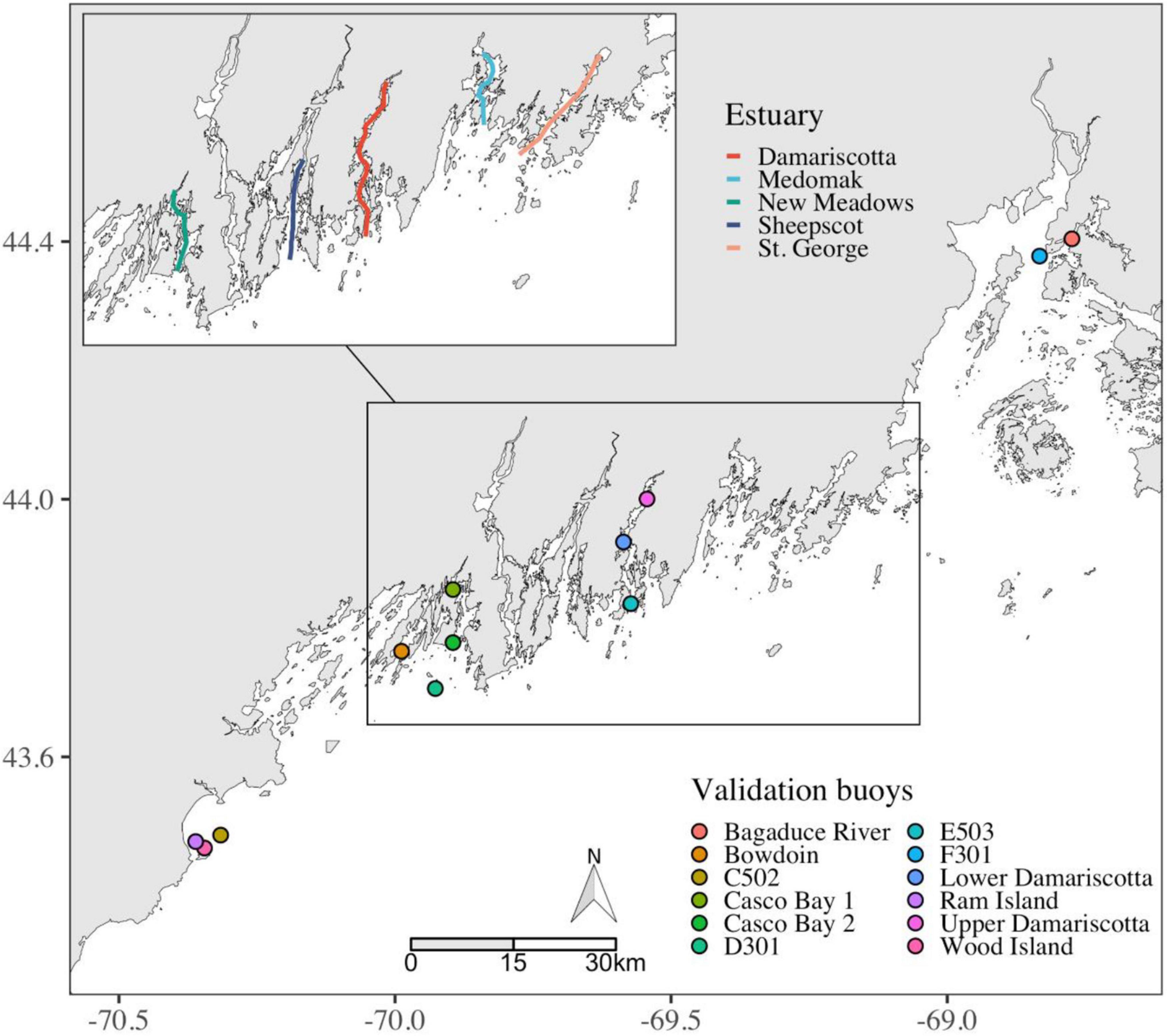
Figure 1. Locations of buoys in the GoM whose environmental data we use for validation of the remote-sensing products computed along five transects in different Maine estuaries.

Satellite Data

Sentinel 2 Level 1C (L1C) top-of-the-atmosphere radiance data were downloaded from CREODIAS.² Thermal Landsat 8 data (Collection 2 Level 2) were downloaded from the USGS earth explorer.³ We obtained 86 Sentinel 2A or 2B images covering all five estuaries from June to September in 2016–2020 and 62 thermal Landsat 8 images from June to September in 2013–2020. We used the images to develop monthly climatologies for the region. The period from June to September was selected because it represents the primary oyster growing season in Maine (Snyder et al., 2017; Adams et al., 2019).

Atmospheric Correction of the Level 1C Data

Atmospheric correction (AC) is a necessary step for processing ocean color imagery as typically > 90% of top-of-the-atmosphere upwelled radiance in the visible spectrum above water is due to the interaction of light with atmospheric aerosols and gas. However, there is currently no consensus regarding the best scheme to perform such AC (Warren et al., 2019; Pahlevan et al., 2021). Therefore, we used five different and freely available AC schemes to derive remote sensing reflectance at sea level, including SeaWiFS Data Analysis System (SeaDAS), Acolite, Polymer, the Case 2 Regional Coast Color processor (C2RCC), and the Ocean Color Simultaneous Marine and Aerosol Retrieval Tool (OCSMART) (Table 1).

TABLE 1

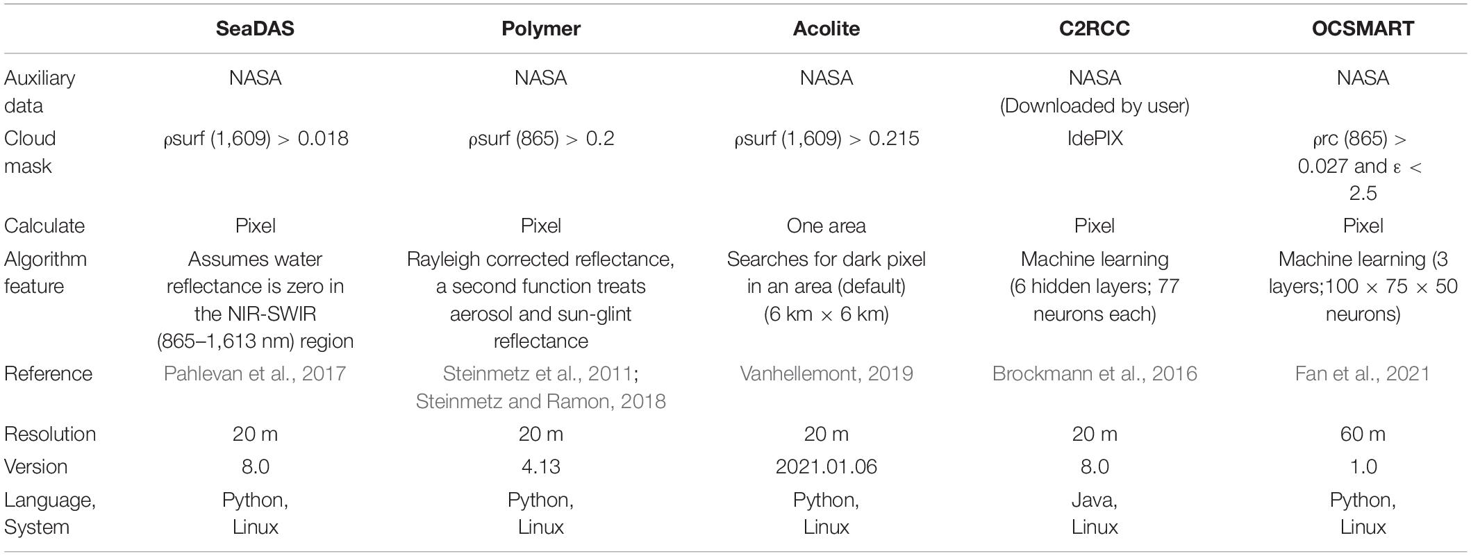
Table 1. Descriptions of the five atmospheric correction schemes (adapted from Pahlevan et al., 2021).

Each AC scheme was processed using the default settings (e.g., no glint correction). For those AC schemes that produce water reflectance (ρ_w), we converted each ρ_w to remote-sensing reflectance (Rrs; unit: sr^–1) by:

$Rrs=\frac{{\mathrm{\rho }}_w}{\mathrm{\pi }}$

The spatial resolution for most of the AC corrected data from Sentinel 2 is 20 m with the exception of OC-SMART which has a resolution of 60 m. For comparison with buoys, we performed statistics on seven-by-seven pixels centered around the buoy when the resolution was 20 m and three by three pixels centered on the buoy when it was 60 m (Pahlevan et al., 2021).

Deriving Suspended Particulate Matter From Atmospheric Correction Corrected Sentinel 2 Images

We chose two algorithms, one explicit (Nechad et al., 2010) and one implicit (SOLID) (Balasubramanian et al., 2020), to derive SPM from Rrs computed from Sentinel 2 (see Supplementary Material for equations). Both algorithms were designed for and applied to locations with SPM concentrations from 0.04 to 110 mg L^–1, which include those found in the GoM (i.e., 0.1–15 mg L^–1).

Deriving Chlorophyll a From Atmospheric Correction Corrected Sentinel 2 Images

We also chose two algorithms to derive Chl a from Sentinel 2 reflectance (see Supplementary Material for equations). The explicit standard OC3/OC4 (OCx) is NASA’s current standard Chl a algorithm (O’Reilly and Werdell, 2019; Pahlevan et al., 2020) and the implicit Mixture Density Networks (MDN) is based on machine learning (Pahlevan et al., 2020). The latter has been found to perform better than the former in an initial analysis of inland and coastal waters (Pahlevan et al., 2020).

Buoy Data for Validation

To validate the remote sensing products, observations from in situ buoys within the region of interest (Figure 1) from the Northeast Regional Association of Coastal Ocean Observing Systems and an aquaculture observing system are available at http://maine.loboviz.com/. The relevant water-quality parameters are Chl a (estimated from measurements with a WETLabs Eco fluorometer), suspended particulate matter (SPM, estimated with a WETLabs Eco FLNTU turbidity meter), fluorescing dissolved organic matter (FDOM, estimated from measurements with a WETLabs Eco fluorometer) and temperature (measured with a SeaBird conductivity and temperature sensor). Although the sensors on these buoys are cleaned regularly, periods with obvious fouling were identified by a trained user and removed.

Comparisons between final satellite data and corresponding buoy measurements were evaluated on their root mean squared error (RMSE), root mean squared log-error (RMSLE), median absolute percentage error (MAPE), mean absolute error computed in log-space (MAE), and log-transformed residuals (Bias) (Tables 2, 3).

TABLE 2

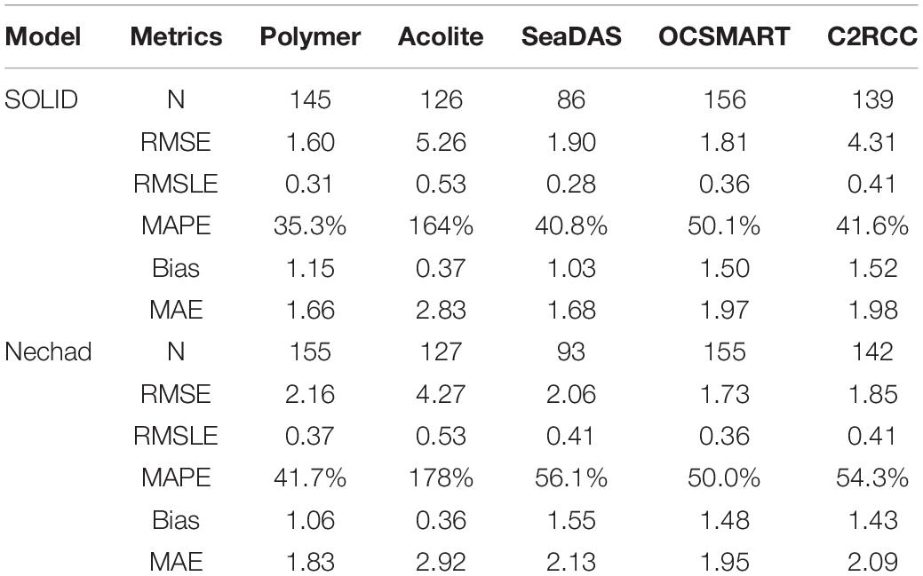
Table 2. Statistical comparisons of SPM derived using five atmospheric correction schemes and buoy data from Supplementary Figure 1.

TABLE 3

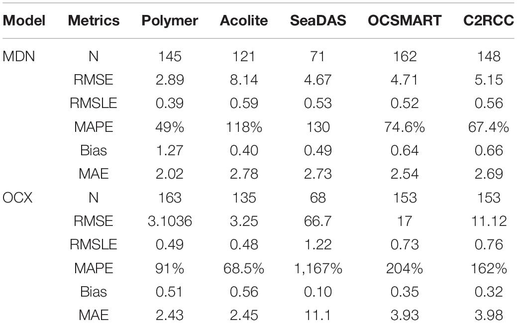
Table 3. Statistical comparisons of Chl a derived using five atmospheric corrections schemes and buoy data from Supplementary Figure 2.

Deriving and Quality Controlling Satellite Temperature Data

Temperature was derived from Landsat 8 collection 2 level 2 by applying a linear formula to the thermal band 10 output.⁴

$SST\left({}^{°}C\right)=Band\mathrm{\hspace{0.25em}10}(K)*0.00341802+149.0-273.15$

We noticed that the cloud mask provided in the level 2 data sometimes misidentified a small number of pixels affected by clouds, cloud shadows, and ice. To minimize SST outliers, we removed pixels out of the 2.5–97.5% range of every satellite scene.

Deriving and Quality Controlling Buoy Suspended Particulate Matter Data

SPM was calculated by converting the turbidity (NTU) reported by the Eco-FLNTU on buoys through a 1:1 relationship, 1 NTU = 1 mg l^–1, although this could vary by up to 37% (Pfannkuche and Schmidt, 2003; Boss et al., 2009; Snyder et al., 2017). Turbidity data were removed from validation data set if a significant drift upward in values was observed before a buoy cleaning. SPM from the Bowdoin buoy in Harpswell, ME (Figure 1) was estimated by calculating the backscatter coefficient (b_b) from the volume scattering function (β) through b_b = 2* π * β(θ) *χ(θ), using an χ(θ) of 1.1 (Boss and Pegau, 2001). Then, SPM was calculated based on the formula from Boss et al. (2009) as follows: NTU = (b_b - bw) /0.0163 where b_w is the backscattering of water.

Deriving and Quality Controlling Buoy Chlorophyll a Data

Chl a concentration estimated with fluorometers (FChl) have to be corrected for several factors including contribution of colored dissolved organic matter (CDOM), variability in the Chl a to FChl relationships, and non-photochemical quenching. CDOM is prevalent in coastal waters and can contribute to the signal measured by Chl a fluorometers (Proctor and Roesler, 2010). We corrected for the CDOM contribution based on the method of Xing et al. (2017):

$FCh{l}_{corrected}=FChl-Y*F\mathrm{\_}CDOM$

Where F_CDOM comes from the DOM fluorometer in Quinine Sulfate units (QSDE) and Y is the slope of the FCHL and CDOM relationship which ranges from 0.04 to 0.11 chl/QSDE, with a mean of 0.087 (Proctor and Roesler, 2010). Additionally, there is natural variability between the relationship of Chl a and its fluorescence. The Chl a fluorometers used here (i.e., WETLabs eco series) have been found to globally overestimate Chl a by a factor of 2 μg l^–1 (Roesler et al., 2017). However, in the GOM, the sensors have been found to underestimate the extracted Chl a by a factor of 1.71 μg l^–1 based on Snyder et al. (2017) and additional unpublished comparisons. We adjusted our estimates with this correction factor. Finally, daytime measurements of FChl often underestimate the true value as phytoplankton quench fluorescence when exposed to high light (termed non-photochemical quenching, NPQ). We mitigated the effects of NPQ through the use of night time buoy measurements (hence measurements that do not suffer from NPQ) taken at the same phase of the tide as satellite overpass. We computed a corrected Chl a estimate from an average of FChl_corrected at 12.5 h before the Sentinel 2 overpass time and 12.5 h after the overpass time. This final adjusted Chl a value was used for validation.

Extracted Chlorophyll-a for Final Algorithm Comparison

Despite the corrections applied in section “Deriving and Quality Controlling Buoy Chlorophyll a Data,” fluorescence remains an imperfect measure of Chl a (Proctor and Roesler, 2010). To determine the final Chl a algorithm, match-ups between Sentinel 2 derived Chl a and extracted Chl a from a long-term monitoring program were made after applying both algorithms, MDN and OCX, to the best performing AC method. The extracted Chl a monitoring program samples surface water twice weekly from a dock at the Darling Marine Center in the Damariscotta River Estuary. Water samples were collected in triplicate in opaque bottles at noon, roughly 1 h after Sentinel 2 overpass, and filtered for a standard acetone extraction before being read on a Turner 10 AU fluorometer (Holm-Hansen and Riemann, 1978).

Derivation of Particulate Organic Matter From Chlorophyll a and Suspended Particulate Matter

Newell et al. (2021) used high resolution satellite imagery and a multiple linear regression to derive particulate organic matter (POM), an indicator of food available to oysters, from SPM and Chl a. Importantly, they argued that this technique is only applicable to coastal environments with low inorganic SPM loads, which is characteristic of the five estuaries we targeted. We derived POM using the following equation from Newell et al. (2021):

$POM=\left(0.153*Chl+0.194*SPM\right)/0.939$

The Oyster Suitability Index

For each of the five estuaries, 3 × 3 pixel transects were extracted from the final water quality products, POM, SPM, Chl a, and temperature. The oyster suitability index (OSI) was computed along the latitude of the transect following Snyder et al. (2017):

$OSI=SS{T}_{weight}*0.8+Ch{l}_{weight}*0.15+SP{M}_{weight}*0.05$

Where each parameter (SST, Chl a, SPM) is attributed a weight if it falls within conditions defined as ideal, moderate or poor for oyster culture (Table 4; Snyder et al., 2017). Each weight was multiplied by its importance factor and added together to calculate the final OSI (Table 4). If any of the parameters fell in the poor classification, the final OSI was reduced to 0. The OSI was classified as poor (OSI < 0.25), moderate (0.25 < OSI < 0.75), and ideal (OSI > 0.75). The weights in Snyder et al.’s (2017) OSI were derived from published literature; however, we acknowledge that they were derived from expert opinion and literature values and designed to be an initial step in classifying productive oyster sites. We included the transects of each environmental parameter used in the OSI so independent conclusions could be drawn.

TABLE 4

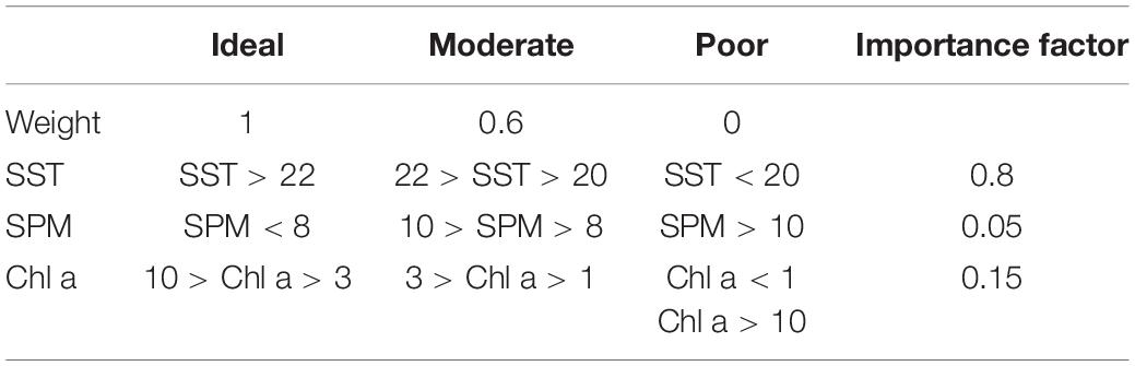
Table 4. Values for oyster suitability index for the Gulf of Maine (adapted from Snyder et al., 2017).

Results

Validation of Remotely Derived Parameters

We compared the different scheme and algorithm combinations with the buoy measurements of SPM and Chl a (Tables 2, 3; see Supplementary Figures 1, 2 for visual comparisons of remote sensing observations and corresponding buoy values). Overall, there were 10 different combinations, five AC methods and two algorithms, for each parameter. The resulting match up performance metrics varied with AC and algorithm.

For SPM, the SOLID algorithm and Polymer AC outperformed the other combinations. Polymer resulted in the lowest MAPE and MAE for both algorithms; however, the SOLID-Polymer combination had 15 and 9 percent lower MAPE and MAE, respectively, when compared to the Nechad-Polymer results (Table 2). Additionally, the SOLID-Polymer comparison had the lowest RMSE and lower or similar RMSLE than the other AC schemes. While the SOLID-Acolite and SOLID-SeaDAS combinations had lower bias than SOLID-Polymer, the SOLID-Acolite combination had four times higher MAPE and a 58% higher MAE (Table 2). The SOLID-SeaDAS’s MAPE and MAE were closer to the SOLID-Polymer combination, however, it produced a 40% reduction in number of matchups.

The MDN algorithm and Polymer AC outperformed the other algorithm-AC scheme combinations when compared to buoy Chl a (Table 3). Similar to the SPM comparisons, MAPE and MAE were lower for both OCx and MDN when processed by Polymer than any other AC scheme, but were lower by 46 and 17 percent for the MDN-Polymer combination. RMSE and RMSLE for the MDN-Polymer combination were also lower than the other MDN-AC scheme combinations. The OCx-Polymer combination had lower RMSE than other OCx-AC scheme combinations, but was slightly outperformed in RMSLE by OCx-Acolite. Overall, the buoy comparisons demonstrated that the Polymer AC scheme provided the lowest error metrics and the Polymer processed MDN Chl a slightly outcompeted the OCx Chl a.

For the final verification of Chl a, products derived from both OCx and MDN on Polymer processed scenes were compared to a time series of extracted Chl a in the Damariscotta River (Figure 2). The same error metrics used to assess the buoy comparisons resulted in much lower MAPE, MAE, and bias for OCx than MDN when compared to extracted data. While RMSE and RMSLE was lower for the MDN algorithm, the Chl a was consistently underpredicted and 70 percent fewer matchups were retrieved than with OCx.

FIGURE 2

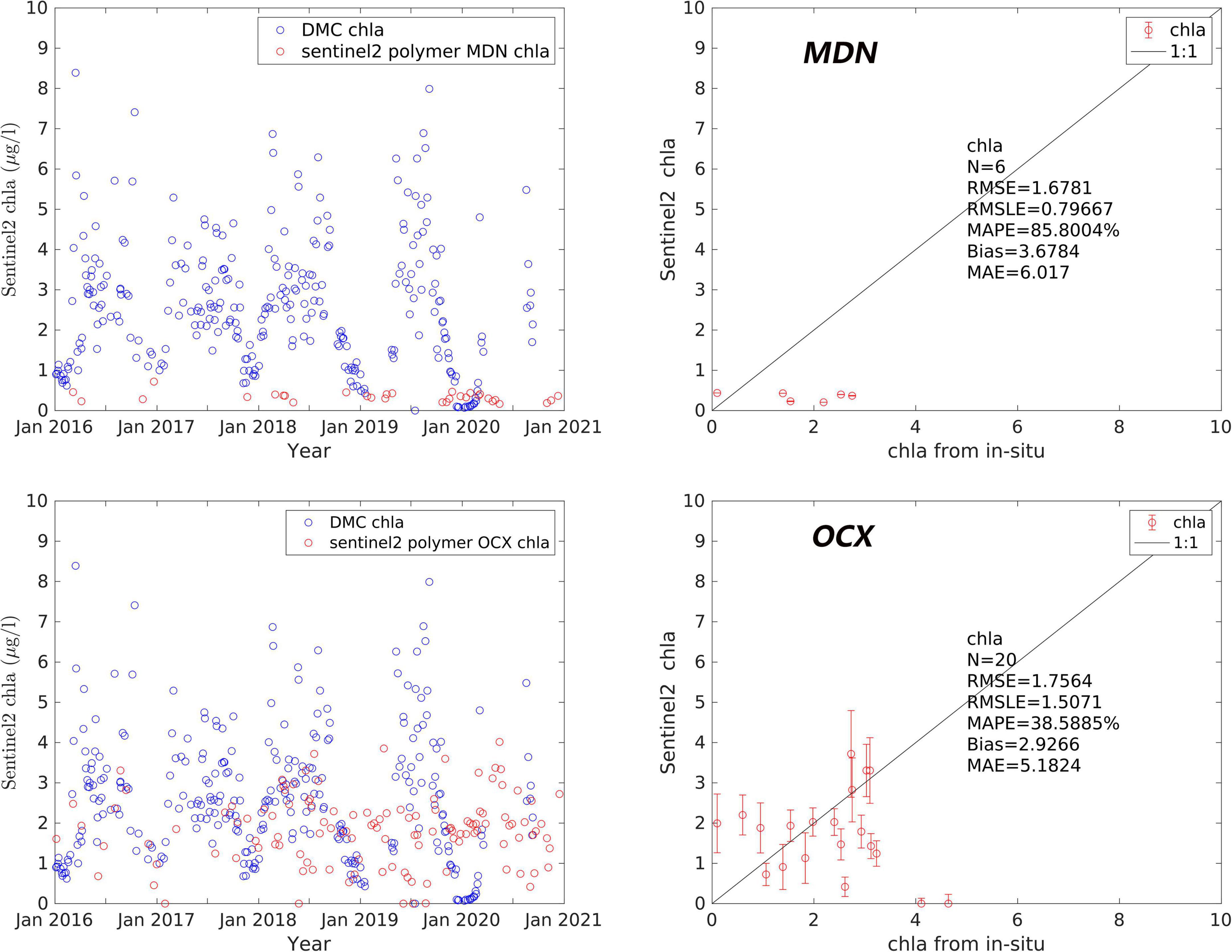
Figure 2. (Left) Time series comparisons of remote sensing Chl a and extracted in-situ Chl a in the Damariscotta River estuary. (Right) Matchups between remote sensing Chl a and time series Chl a. All satellite derived Chl a was Polymer processed and Chl a was derived from the MDN (top) or OCx (bottom) algorithms.

For the examinations of oyster aquaculture suitability all scenes were corrected with Polymer, the SOLID algorithm was used to generate SPM, and the OCx algorithm was used to derive Chl a. We also validated the Landsat 8 SST product and found it satisfactory (e.g., RMSE < 1.3°C) (Hesketh, 2021).

Transects of Five Study Estuaries

In the Damariscotta River estuary, the single largest oyster growing area in the Northern New England region, the median summer SST ranged from 16°C at the mouth of the estuary to 23°C in its upper reaches, the highest median temperatures observed in the study (Figure 3). Chl a was consistent at 2 μg l^–1 up to latitude 43.97°N north of which it increased to a peak at ∼ 4 μg l^–1. SPM slowly increased from a median of 1 mg l^–1 at the mouth to 1.5 mg l^–1 at the upper end of the estuary (Figure 3). The majority of the Damariscotta scored a low OSI due to low temperatures. However, above 44.97°N, the estuary became better suited for oyster culture as the temperature increased from a poor to a moderate classification. The very upper portion of the Damariscotta (above latitude 44.01°N) is the only area in this analysis that reaches OSI values of 1 driven by high temperature and moderate food conditions. No other estuary reached median temperatures above 22°C, capping the highest possible OSI values in other estuarine systems at 0.68 (Figures 3–6).

FIGURE 3

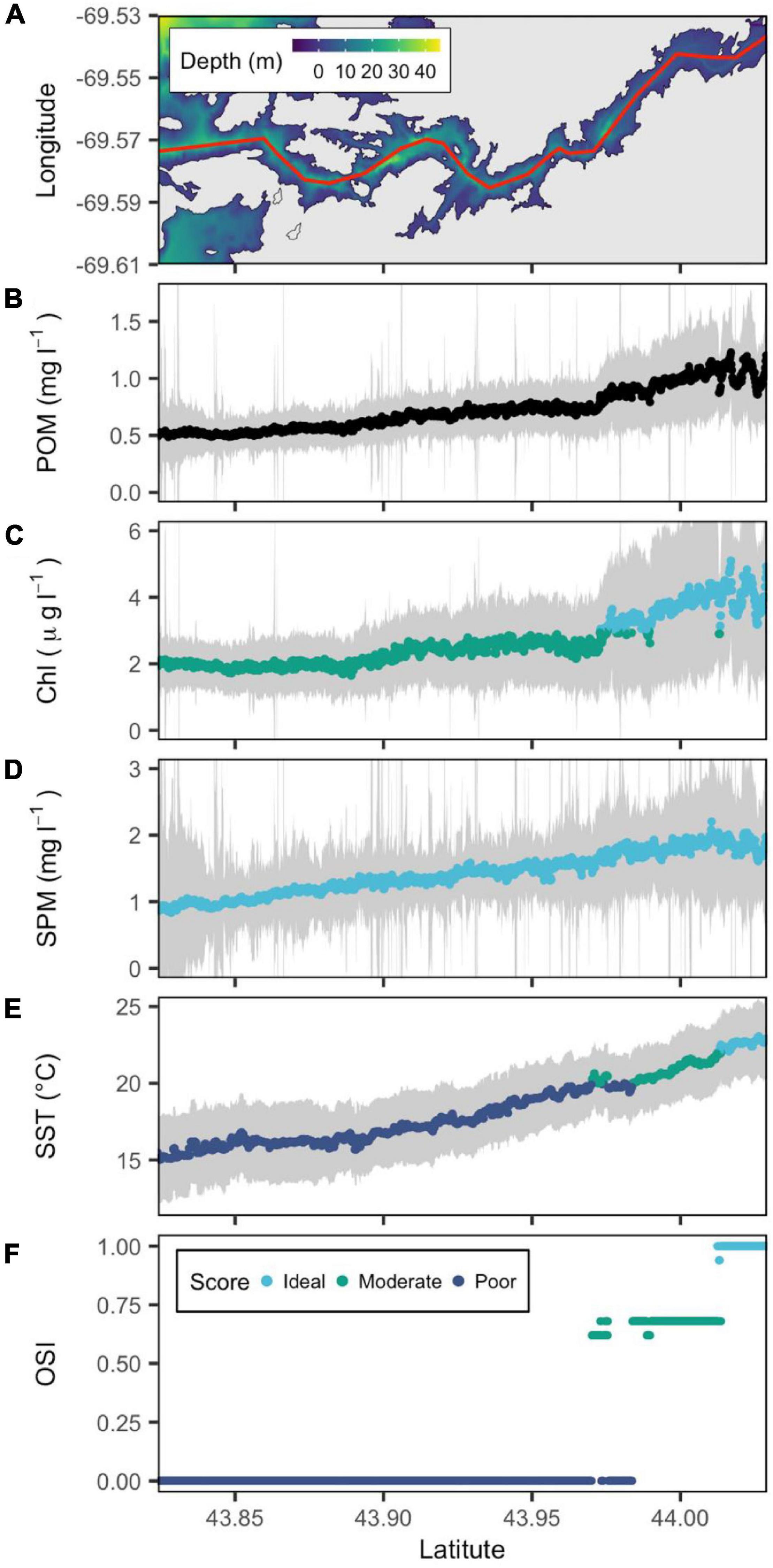
Figure 3. Bathymetric map of the Damariscotta River estuary (from downstream to upstream left to right) with a red line showing the central transect. (A) POM (B), SPM (C), Chl a (D), and SST (E) are reconstructed from remote sensing data, and OSI (F) is derived following the method of Snyder et al. (2017). Gray color belts show standard deviation of POM, SPM, Chl a, and SST derived in summer (June–September) over the period 2016–2020, with their median values depicted by blue, green, and cyan points that denote poor, moderate and ideal conditions for oyster aquaculture, respectively.

FIGURE 4

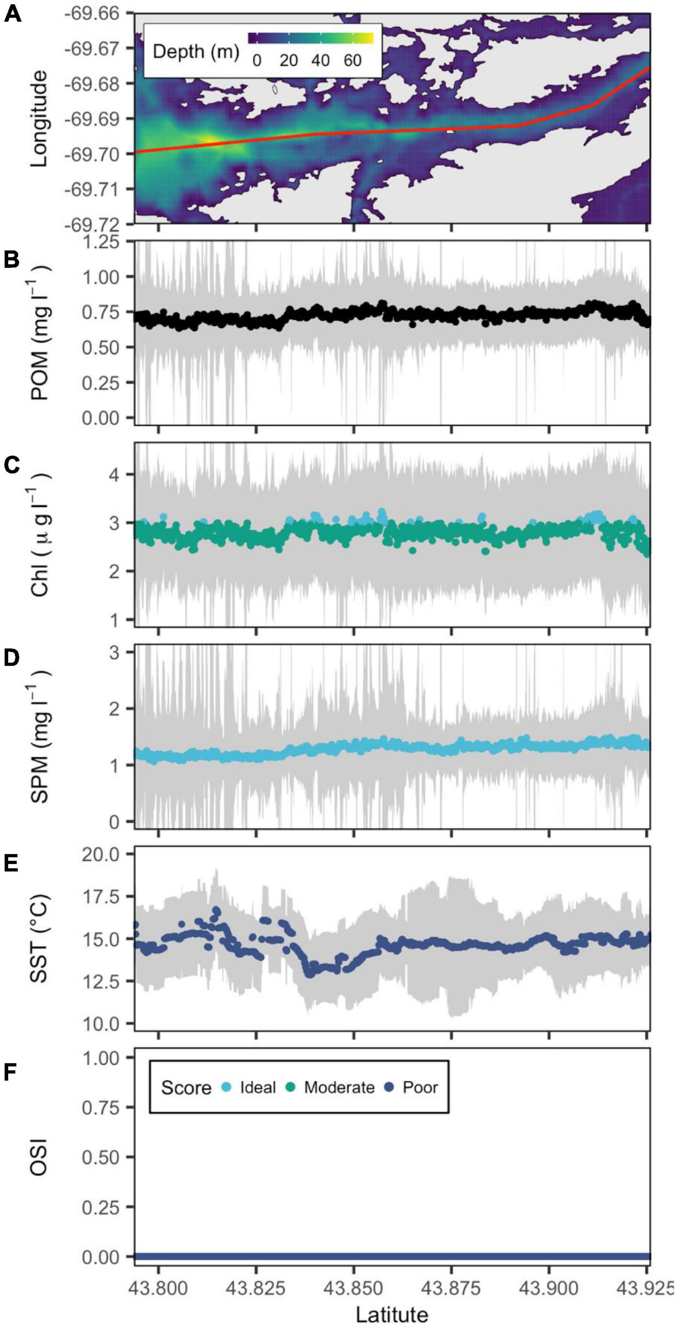
Figure 4. Bathymetric map of the Sheepscot River estuary (from downstream to upstream left to right) with a red line showing the central transect. (A) POM (B), SPM (C), Chl a (D), and SST (E) are reconstructed from remote sensing data, and OSI (F) is derived following the method of Snyder et al. (2017). Gray color belts show standard deviation of POM, SPM, Chl a, and SST derived in summer (June–September) over the period 2016–2020, with their median values depicted by blue, green, and cyan points that denote poor, moderate and ideal conditions for oyster aquaculture, respectively.

FIGURE 5

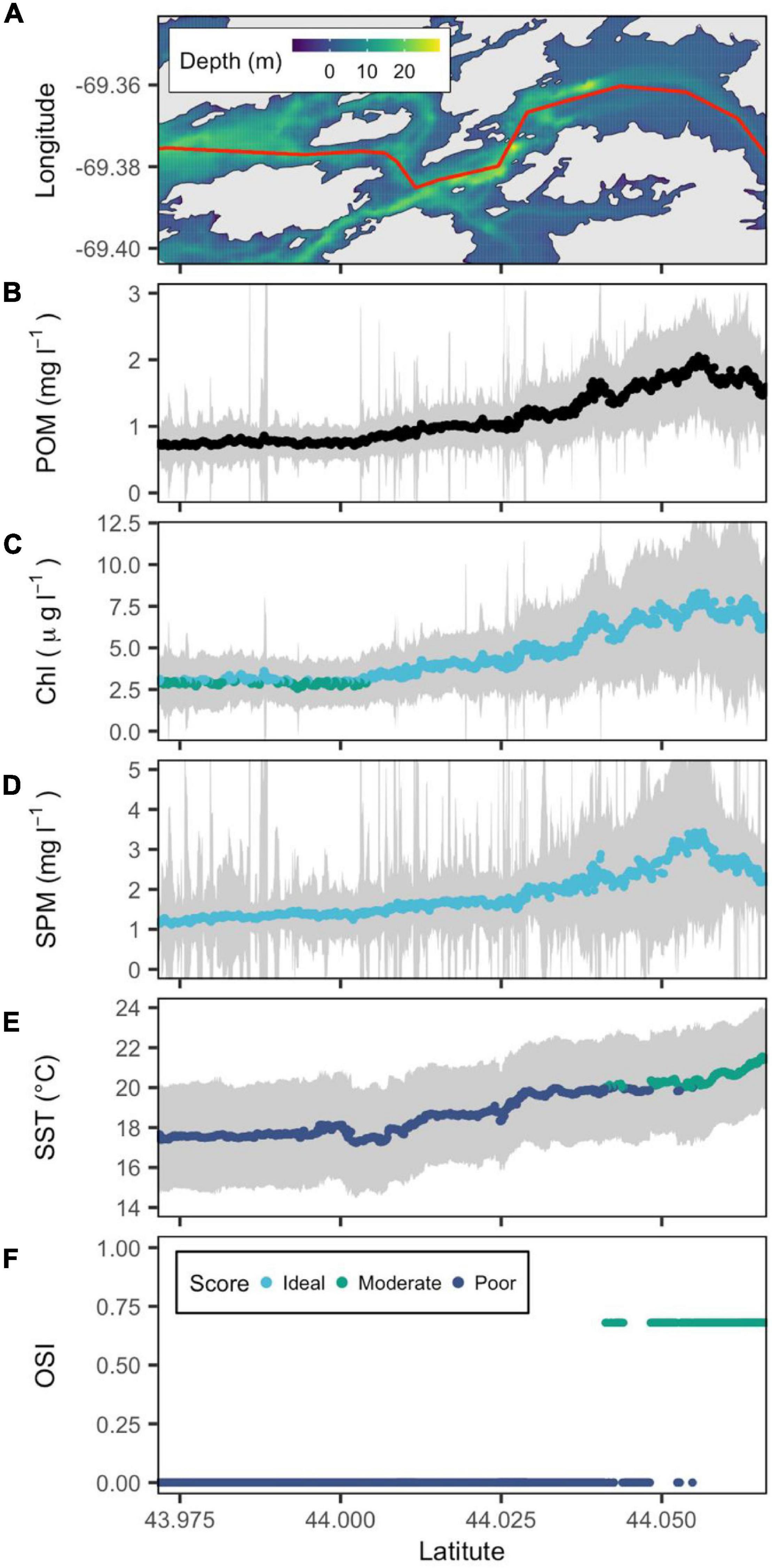
Figure 5. Bathymetric map of the Medomak River estuary (from downstream to upstream left to right) with a red line showing the central transect. (A) POM (B), SPM (C), Chl a (D), and SST (E) are reconstructed from remote sensing data, and OSI (F) is derived following the method of Snyder et al. (2017). Gray color belts show standard deviation of POM, SPM, Chl a, and SST derived in summer (June–September) over the period 2016–2020, with their median values depicted by blue, green, and cyan points that denote poor, moderate and ideal conditions for oyster aquaculture, respectively.

FIGURE 6

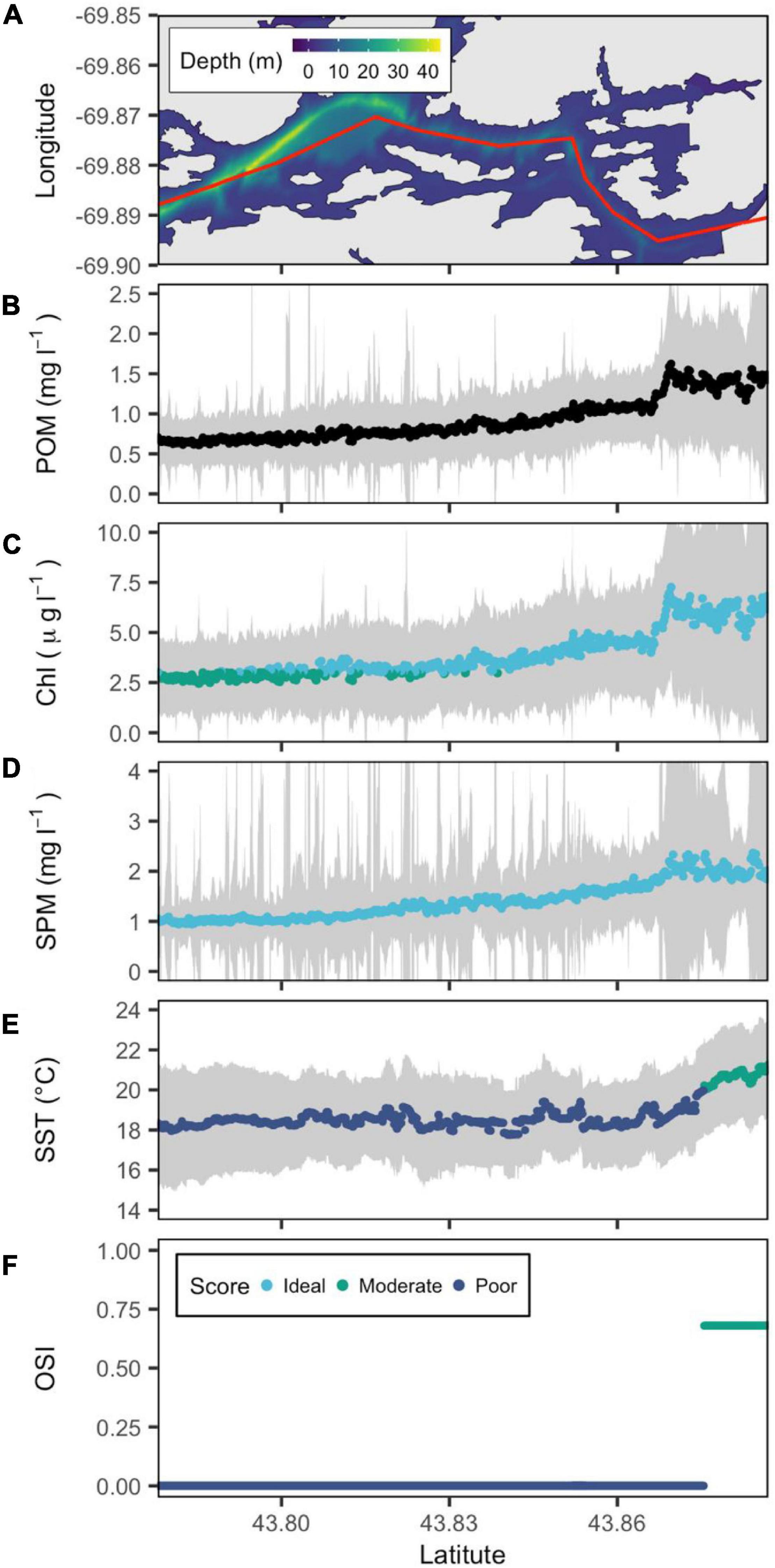
Figure 6. Bathymetric map of the New Meadows River estuary (from downstream to upstream left to right) with a red line showing the central transect. (A) POM (B), SPM (C), Chl a (D), and SST (E) are reconstructed from remote sensing data, and OSI (F) is derived following the method of Snyder et al. (2017). Gray color belts show standard deviation of POM, SPM, Chl a, and SST derived in summer (June–September) over the period 2016–2020, with their median values depicted by blue, green, and cyan points that denote poor, moderate and ideal conditions for oyster aquaculture, respectively.

In contrast to the Damariscotta, OSI values in the Sheepscot River estuary indicated that the majority of its main channel is unsuitable for oyster culture. Throughout the Sheepscot transect, the median SST ranged from 13 to 16°C with no warming trend with latitude. Similarly, SPM remained constant at a relatively low 1 mg l^–1 along the entire estuary (Figure 4). Chl a is also constant along the transect with concentrations just under 3 μg l^–1. Occasionally, Chl a crosses into the moderate classification raising the OSI values to 0.2 (Figure 4). Due to the low Chl a and SPM concentrations, the Sheepscot had the lowest satellite derived POM of the estuaries in our analysis (Figures 3–7).

FIGURE 7

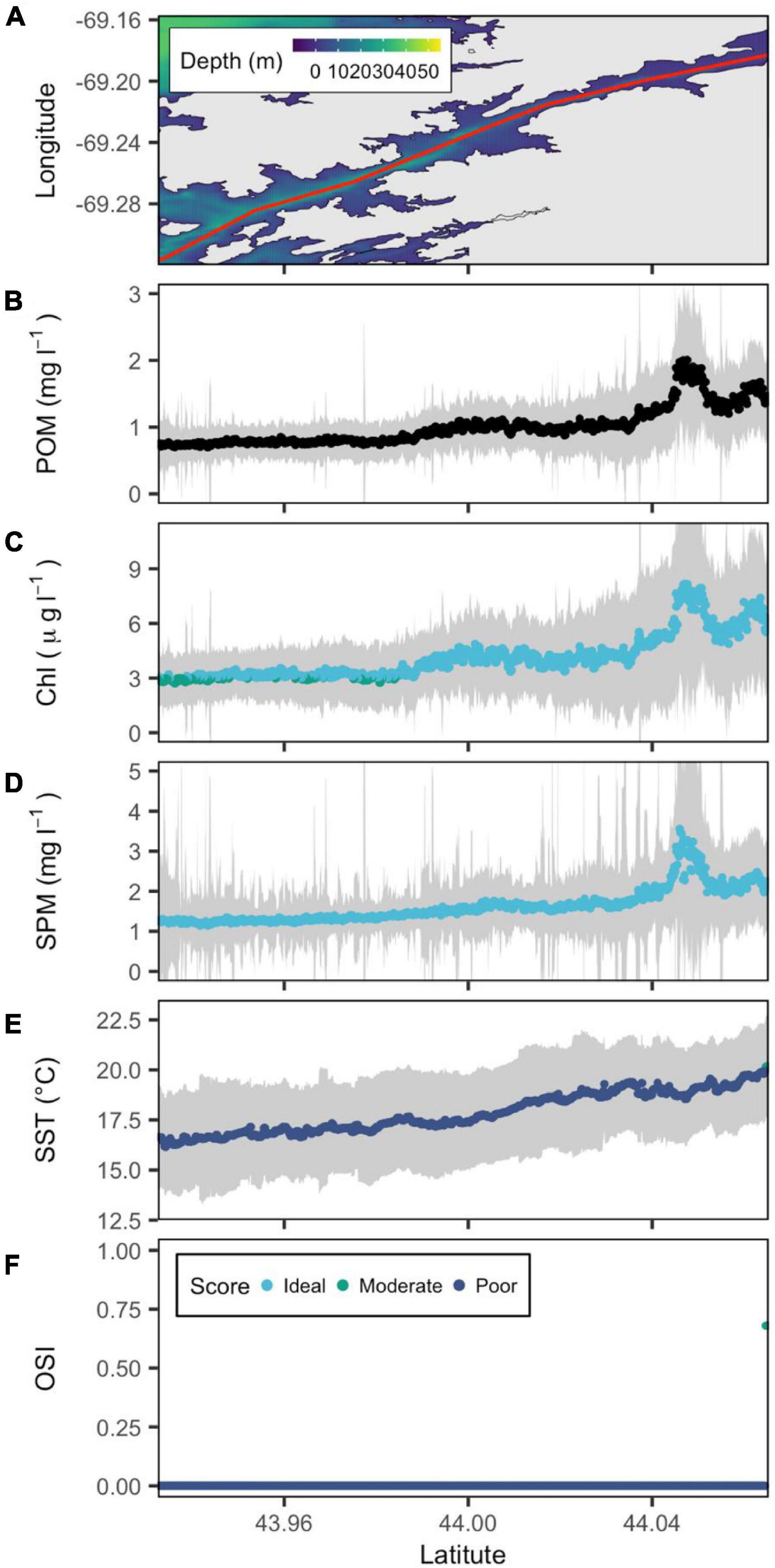
Figure 7. Bathymetric map of the St. George River estuary (from downstream to upstream left to right) with a red line showing the central transect. (A) POM (B), SPM (C), Chl a (D), and SST (E) are reconstructed from remote sensing data, and OSI (F) is derived following the method of Snyder et al. (2017). Gray color belts show standard deviation of POM, SPM, Chl a, and SST derived in summer (June–September) over the period 2016–2020, with their median values depicted by blue, green, and cyan points that denote poor, moderate and ideal conditions for oyster aquaculture, respectively.

The temperature conditions in the shallower Medomak were more favorable to oyster aquaculture ranging from 18°C at the mouth to 22°C further inland (Figure 5). The Medomak also exhibited the highest sustained concentrations of bivalve food. Chl a could be as high as 5 μg l^–1 and SPM ∼3 mg l^–1 between 44.05 and 44.06°N (Figure 5). The relatively high Chl a and SPM also resulted in the highest calculated POM values observed in mid-Coast GoM (Figure 5).

Although located ∼ 45 km to the southwest, the New Meadows River estuary was very similar to the Medomak. The temperature transects the same range (18–22°C). Chl a was slightly lower, reaching ∼7 mg l^–1 at the highest point along the transect with the corresponding peak in SPM reaching 2 mg l^–1 (Figure 6). Above latitude 43.87°N, the OSI reached its peak of 0.68, driven by higher food availability and moderate temperatures (Figure 6).

The most northeastern estuary, the St. George, had similarly low OSI values and spatial homogeneity as the Sheepscot for the majority of the system. However, while the Sheepscot has consistently low temperature and food along the entire transect, the St. George does show a pattern of increasing conditions with higher latitudes. SST increased to just over 20°C at the very top of the estuary from 16°C at the mouth. St George Chl a and SPM increased from 1.5 and 1.5 mg l^–1, respectively, to a small peak of 8 and 3 mg l^–1 at similar latitudes to the Medomak (Figure 7).

Discussion

Proposed Methods for Deriving Remote Sensing Data

We compared five atmospheric corrections with two algorithms for each derived parameter (Chl a and SPM) and found the combination that provided the best comparison with available in situ data. It is important to note that variability between the CDOM to Chl a ratio in a given environment and the environment the algorithm was trained in can cause poor performance. This variability often drives many practitioners to use local data to design their own regional Chl a algorithm. Another cause for poor Chl a comparisons in Sentinel 2 Chl a products are across track non-uniformities created by instrument artifacts identified in Pahlevan et al. (2017). Comparisons between remote sensing imagery and buoy-based observations located in different tracks of the same image may result in over- or under-estimations because the conditions under which they are captured are not identical and inaccuracies in the AC procedure can thus result in striped composites. Note that in this work, we are not using locally tuned algorithms but rather algorithms developed by other groups with data encompassing a variety of environments to reflect the conditions that the vast majority of aquaculturists would potentially access remote sensing imagery during their decision-making process.

Combining ocean color data with SST from Landsat 8 and averaging over several years to obtain enough images to create a stable climatology allowed us to compute the distribution of POM and the OSI for five estuaries in the mid-coast of the GoM, from which promising new areas for oyster aquaculture can be identified. For example, the Medomak River estuary has relatively few aquaculture leases; however, conditions from our analysis indicate that this region is a promising location for sustainable oyster aquaculture development.

The ability to accurately characterize spatial transects in water quality at high spatial resolution should improve as more cloud free imagery becomes available. However, there are caveats to using this information and recommendations for improvement. The accuracy of water quality parameters was strongly linked to the suitability of the atmospheric correction applied (Supplementary Figures 1, 2). So far, there are no AC schemes that perform best for high resolution satellites everywhere, e.g., contrast Warren et al. (2019) with Pahlevan et al. (2021). The search for a more universal or flexible AC scheme may be improved if data from other sources (e.g., AERONET-OC and other satellites) are brought to bear on this problem (Warren et al., 2019; Pahlevan et al., 2021).

Food and the Oyster Suitability Index

The OSI is driven primarily by temperature which is weighted at 80% of the final value. Temperature and food are often regarded as the main drivers of oyster growth (Bourlès et al., 2009; Rico-Villa et al., 2009; Hawkins et al., 2013a; Filgueira et al., 2014). Temperature is especially important in GoM oyster culture since it is close to the northern end of the eastern oyster’s range. Eastern oyster filtration activity is generally minimal below 10°C and increases to a peak at roughly 30°C (Loosanoff, 1958) with optimal temperatures falling between 20 and 30°C (Stanley and Sellers, 1986). When temperature is low enough to reduce feeding, oysters may not need to take advantage of all available food, indicating that at higher temperatures food becomes more important (Comeau et al., 2008, 2010). Median growing season Chl a, the proxy for oyster food in the OSI, varied from 2 to 8 μg l^–1 along transects and between estuaries. While all the study estuaries had regions classified as poor based on food (Figures 3–6), in all regions where temperature fell within the moderate and ideal temperature ranges (>20°C), Chl a was primarily in its ideal range (3–10 μg l^–1) indicating that food was not a major limiting parameter in the identification of sites with the OSI.

Low summer SPM concentrations were observed in all five estuaries with a max of ∼ 6 mg l^–1. Low SPM was likely due to the minimal freshwater input in all the systems reducing input from terrestrial sources. Snyder et al.’s (2017) OSI includes high concentrations of SPM as a negative parameter for oyster growth due to the potential for the inorganic components of SPM to dilute bivalve food (Widdows et al., 1979; Barille et al., 1997; Snyder et al., 2017). However, while oysters and other bivalves have been shown to preferentially select phytoplankton, they also gain significant energy from detrital components in POM (Langdon and Newell, 1990; Hawkins et al., 2013a,b; Both et al., 2020). Within our study area, bioavailable proteins within detritus are an important and necessary source of protein for oysters in the Damariscotta River (Adams et al., 2019). In a study examining oyster feeding rates in the upper Damariscotta River estuary, one of the most productive oyster producing regions in Maine, POM averaged 1.8 mg l^–1 (±0.8) over the growing season (Adams et al., 2019). While not included in the OSI, we calculated POM transects to give a more complete picture of bivalve food to account for the likely positive contribution of detritus in these systems with low freshwater input and consequently, low inorganic sediment load. Where the transect temperatures are above 20°C, POM is above 1 mg l^–1, similar to the upper Damariscotta (Figures 3–6). Furthermore, the good correspondence between SPM and Chl a along with their moderate values are also encouraging as they suggest that SPM is mostly organic in origin and likely representative of food as opposed to transported or resuspended terrestrial sediments of low or no nutritional value.

Oyster Aquaculture Site Prospecting

Mid-coast GoM estuaries examined for oyster aquaculture suitability fall in a region dominated by narrow North-South running estuaries formed from drowned river valleys bounded between Casco Bay in the South and Penobscot Bay in the North (Kelley, 1987). Despite all five of the estuaries entering the GoM along a 50 km stretch of coast, depth and natural constrictions can lead to variations in mixing and residence time. There are relatively few published estimates of residence time for these systems; however, it has been examined in some of the study estuaries. Geomorphological features in the upper Damariscotta result in long residence times (>7 days, Liberti et al., 2021). Hillyer et al. (2021) also recently calculated residence times for the Medomak River estuary on the order of days. Conversely, the mouths of these same estuaries tend to have residence times on the order of one to two tidal cycles (Liberti et al., 2021). Clearly, our transects reflect the spatial change in residence time of these long narrow estuarine systems where bottom and side friction retains water and particulates at the upper end of the estuaries and flushes relatively rapidly at the mouth. These variations can create significant variations in temperature and oyster food between and along transects of these systems. Finally, in contrast, estuarine systems without these geomorphological features, such as the Sheepscot and St. George estuaries, displayed spatially homogeneous patterns in temperature and food availability suggesting relatively low residence time for heat and particulate retention.

Comparisons between existing farm sites and the OSI allow for additional observational validation of its performance. The Damariscotta River estuary (DRE; Figure 3) and the New Meadows (Figure 6) are regions of relatively high current production in both our analysis and actual production. Maine’s regulation of aquaculture leases can be grouped into larger standard or experimental leases (referred to as leases) and smaller limited purpose aquaculture leases (referred to as LPAs). The size of an LPA is capped at 37 square meters and is designed for potential farmers to trial farm sites before starting the costly process of obtaining a lease. The DRE and the New Meadows contain both lease types.

Oyster aquaculture in the region began in the DRE in 1975 (Hanes, 2019) and now produces over half of Maine oysters from 29 leases held by 13 farms as well as 74 LPAs (Maine Department of Marine Resources, 2021). The majority of these DRE farms are concentrated in the upper third of the estuary above latitude 43.9°N. At this location, a natural bedrock constriction separates the upper DRE from the remaining estuary increasing the residency time of the water and allowing it to warm to ideal temperatures for oyster aquaculture. The increased suitability of the upper estuary for warm water culture species has been well documented (Shatkin, 1992; Barber and Davis, 1997; Snyder et al., 2017; Beard et al., 2020). One early study showed 25 mm difference in shell length and a 40 g difference in live weight of eastern oysters after one growing season compared to a site only 7.5 km south of the estuary’s constriction (Davis and Barber, 1999). Promisingly, the satellite derived OSI captured the effects of the constriction with the OSI reaching moderate classification at the same latitude as the constriction and increasing to the only ideal classification in the main growing area (Figure 3).

While aquaculture development in the New Meadows is relatively new compared to the Damariscotta and hosts fewer farm than the Damariscotta, the five leases held by five separate farms as well as 47 LPAs indicate high interest in oyster culture and make it a good test case for the satellite driven OSI (Maine Department of Marine Resources, 2021). These standard leases are all held above latitudes of 43.87°N, within the area identified as suitable by the OSI (Figure 6). While the majority of the LPAs are also concentrated in the upper estuary, many are held in latitudes with low OSI values, but are close to shore or in coves that may offer warmer water temperatures. A valuable application of high-resolution satellite products may be lateral transects in addition to the latitudinal transects we have focused on here.

While the Damariscotta and the New Meadows are established hubs of oyster culture, the three remaining estuaries examined are largely unused by farmers. The Sheepscot has 5 leases and 14 LPAs, the Medomak has one lease and no oyster LPAs, and the St. George has one lease and 14 LPAs (Maine DMR). In these regions the OSI can be used for prospecting lease sites.

Results for the Sheepscot deemed it largely unsuitable for eastern oyster culture (Figure 4). While similar in size to the Damariscotta, the lower portion of the Sheepscot is characterized by a deep (MLW 20–60 m) channel and well mixed cold waters (Stickney, 1959). In the summer months, the majority of the river is ∼5–10°C colder than the DRE (Figures 3–7). However, in the upper reaches of the estuary the water becomes shallower (MLW 1–10 m) and the river experiences a wider range of temperatures and is more influenced by its two main tributaries, the Marsh and Dyer Rivers (Stickney, 1959). In this upper portion, beyond the range of the transect, there is a large oyster farm that consists of 4 of the 5 leases in the river at latitude 44.03°N (Maine Department of Marine Resources, 2021) as well as one of the few natural populations of C. virginica in Maine (Larsen et al., 2013). Given the low concentrations of Chl a and POM as well as the lowest summer temperatures in this study, the lower Sheepscot may be more suitable for culture of mussel or scallop species that prefer temperature in the 10–20°C and Chl a above 0.5 mg l^–1 (Mizuta and Wikfors, 2019; Coleman et al., 2022).

Similar to the Sheepscot, the majority of the St. George also scored low on the OSI. This estuary is oriented on a Northeast-Southwest line compared to the other North-South estuaries in this study and is the last major estuary before Penobscot Bay, marking an important demarcation between Eastern and Western GoM source water to these estuaries (Figure 1). Like the Sheepscot, the St. George is connected to the GoM by a deeper channel resulting in colder water infiltrating deeper into the estuary (Maine Coastal Observing Alliance [MCOA], 2015). However, unlike the Sheepscot, the food and temperature conditions improve with higher latitudes. Currently, the northernmost farm site is a recreational LPA at 44.01°N and oyster sites are present as far South as 43.94°N (Maine Department of Marine Resources, 2021). While the OSI scores the majority of the upper river as poor growing locations, the median temperatures are ∼19°C and coupled with the high food, may present productive growing locations.

The Medomak River had the fewest number of oyster leases and LPAs despite relatively high OSI scores. The system plays a key role in the state’s clam fishery, the second largest fishery in the region to American lobster (Hillyer et al., 2021). The estuary has a wide mouth where it enters the GoM and narrows to a constriction at ∼44.01°N after which it widens to expansive tidal flats with a deep center channel (MLW 6–20 m) (Hillyer et al., 2021). The only oyster lease in the estuary is located at the southern end of the transect in Figure 6 at 43.98°N. While this location is labeled as poor by the OSI, this farm is enclosed within an lobster pound which artificially increases residence time and has been able to produce good growth due to its local environmental conditions (Leeman et al., in review). North of this lease, high Chl a and increased temperatures drive the OSI into moderate values (Figure 6). At high tides, water fills the shallow flats where it can be influenced more heavily by the air temperature (Kim et al., 2010). In the summer, higher air temperatures could lead to warmer waters on ebb tides increasing the OSI. These areas are potentially productive oyster areas; however, close collaboration with existing industries, such as clam harvesters, would be vital in siting farms to avoid conflict (Cleaver et al., 2018).

While the satellite driven OSI provides a valuable tool to inform site selection, the index does not have much flexibility in classifying sites that exist on the borders between classification breaks (such as sites with median temperatures of 19°C), lateral variability across estuaries, or interannual variability. For example, in a 2003 growth study that examined oyster production of selected lines in several estuaries, including the New Meadows and the St. George, Rawson and Feindel (2012) found that the two estuaries had similar whole weight growth (Rawson and Feindel, 2012). However, in a 2004 trial, the New Meadows had roughly double the whole weight as the St. George (Rawson and Feindel, 2012). Despite this variability, satellite derived site selection tools provide valuable spatial data previously unavailable to prospective oyster aquaculturists in a rapidly changing GoM.

Future work should couple process based growth models with remotely sensed parameters and incorporate newly launched satellites. Growth models driven by satellite data can provide metrics such as time-to-market that can be more informative when prospecting for new culture sites (Palmer et al., 2020). Additionally, the new satellite Landsat 9, launched in September 2021, will be able to increase the revisit time of a satellite with thermal bands when combined with Landsat 8 (currently 16 days). When combined with Sentinel 2 (5 days), the high-resolution satellite revisiting time will be 2–3 days providing a greater chance of cloud free overpass days and more robust estimates of seasonal and interannual trends in SST, SPM, and Chl a.

Conclusion

Satellite derived SPM, chlorophyll a, and particulate organic matter from Sentinel 2 and sea surface temperature from Landsat 8 are powerful tools for oyster aquaculture site selection. Using validated remote sensing data from Landsat 8 and Sentinel 2, we mapped the location where oyster aquaculture should thrive along transects of five estuaries in the GoM. The OSI was capable of successfully identifying areas where existing successful farms are already operating as well as identifying a variety of new sites where oyster aquaculture could be successful. The high-resolution products were also capable of detecting the effect of local geomorphological features that drive local scale site selection. A key to the approach is validation with in situ data, as without such validation it is impossible to assess uncertainties of any scheme to derive water quality parameters from the freely available satellite data.

Data Availability Statement

The original contributions presented in the study are included in the article/Supplementary Material, further inquiries can be directed to the corresponding author/s.

Author Contributions

EB, DB, and DF acquired the funding and provided contributions for the design of the work. BJ contributed five ACs and five river OSI and wrote the original draft. GB and GH provided the code of polymer, SeaDAS and Landsat 8 SST. DB was responsible for conducting buoy maintenance in the Gulf of Maine. TK contributed Figure 1 and contributed to the discussion of the five rivers OSI. All authors contributed to the writing of the revised manuscript and the answers to the reviewer’s comments.

Funding

This project was supported by the National Sea Grant award E-14-EA-2, the National Science Foundation award #11A-1355457 to Maine EPSCoR at the University of Maine, the NASA Ocean Biology and Biogeochemistry program Grant #NNX14AP66G, and the NASA EPSCoR program to Maine Space Grant. We also thank the China Scholarship Council (No. CSC201906260052) and the National Natural Science Foundation of China (41976070). Funding was also provided by the Aquaculture Research Institute in partnership with the University of Maine and the USDA Aquaculture Experimental Station. This project was supported by the USDA National Institute of Food and Agriculture, Hatch Project number ME0-830-31000-004-00D through the Maine Agricultural & Forest Experiment Station. Maine Agricultural and Forest Experiment Publication number 3889.

Conflict of Interest

The authors declare that the research was conducted in the absence of any commercial or financial relationships that could be construed as a potential conflict of interest.

Publisher’s Note

All claims expressed in this article are solely those of the authors and do not necessarily represent those of their affiliated organizations, or those of the publisher, the editors and the reviewers. Any product that may be evaluated in this article, or claim that may be made by its manufacturer, is not guaranteed or endorsed by the publisher.

Acknowledgments

We thank Marco Peters Support for C2RCC atmospheric correction by SNAP. Francois Steinmetz support for Polymer, Quinten Vanhellemont support for Acolite, and Yongzhen Fan support for OCSMART. We thank to Stephen Cousins, and Forrest Flagg from the University of Maine high performance computing center. We thank to Bob Fleming for providing the old buoy and Elisabeth Maxwell for providing the calibration data from the new buoy. We thank to the SEANET project at University of Maine for providing LOBO buoy data. We thank to Nima Pahlevan and Brandon Smith for assistance with MDN and SOLID. We thank to Nils Haëntjens for assistance with data processing. Finally, we thank Denghui Li and Kelly Cole for providing the coastline and water depth in Gulf of Maine and Casco Bay, respectively.

Supplementary Material

The Supplementary Material for this article can be found online at: https://www.frontiersin.org/articles/10.3389/fmars.2022.802438/full#supplementary-material

Footnotes

1. ^ www.maine.gov/dmr/
2. ^ https://discovery.creodias.eu/dataset
3. ^ https://earthexplorer.usgs.gov/
4. ^ https://www.usgs.gov/core-science-systems/nli/landsat/landsat-collection-2-level-2-science-products

References

Adams, C. M., Mayer, L. M., Rawson, P., Brady, D. C., and Newell, C. (2019). Detrital protein contributes to oyster nutrition and growth in the Damariscotta estuary, Maine, USA. Aquacult. Environ. Interact. 11, 521–536. doi: 10.3354/aei00330

CrossRef Full Text | Google Scholar

Balasubramanian, S. V., Pahlevan, N., Smith, B., Binding, C., Schalles, J., Loisel, H., et al. (2020). Robust algorithm for estimating total suspended solids (TSS) in inland and nearshore coastal waters. Remote Sens. Environ. 246:111768. doi: 10.1016/j.rse.2020.111768

CrossRef Full Text | Google Scholar

Barber, B. J., and Davis, C. V. (1997). Growth and mortality of cultured bay scallops in the Damariscotta River, Maine (USA). Aquacult. Int. 5, 451–460.

Google Scholar

Barille, L., Prou, J., Heral, M., and Razet, D. (1997). Effects of high natural seston concentrations on the feeding, selection, and absorption of the oyster Crassostrea gigas (Thunberg). J. Exp. Mar. Biol. Ecol. 212, 149–172. doi: 10.1016/S0022-0981(96)02756-6

CrossRef Full Text | Google Scholar

Beard, K., Kimble, M., Yuan, J., Evans, K. S., Liu, W., Brady, D., et al. (2020). A method for heterogeneous spatio-temporal data integration in support of marine aquaculture site selection. J. Mar. Sci. Eng. 8:96. doi: 10.3390/jmse8020096

CrossRef Full Text | Google Scholar

Boss, E., and Pegau, W. S. (2001). Relationship of light scattering at an angle in the backward direction to the backscattering coefficient. Appl. Opt. 40:5503. doi: 10.1364/AO.40.005503

PubMed Abstract | CrossRef Full Text | Google Scholar

Boss, E., Taylor, L., Gillbert, S., Gundersen, K., Hawley, N., Janzen, C., et al. (2009). Comparison of inherent optical properties as a surrogate for particulate matter concentration in coastal waters. Limnol. Oceanogr. 7, 803–810. doi: 10.4319/lom.2009.7.803

CrossRef Full Text | Google Scholar

Both, A., Byron, C. J., Costa-Pierce, B., Parrish, C. C., and Brady, D. C. (2020). Detrital subsidies in the diet of Mytilus edulis; macroalgal detritus likely supplements essential fatty acids. Front. Mar. Sci. 7:561073. doi: 10.3389/fmars.2020.561073

CrossRef Full Text | Google Scholar

Bourlès, Y., Alunno-Bruscia, M., Pouvreau, S., Tollu, G., Leguay, D., Arnaud, C., et al. (2009). Modelling growth and reproduction of the Pacific oyster Crassostrea gigas: advances in the oyster-DEB model through application to a coastal pond. J. Sea Res. 62, 62–71. doi: 10.1016/j.seares.2009.03.002

CrossRef Full Text | Google Scholar

Brockmann, C., Doerffer, R., Peters, M., Kerstin, S., Embacher, S., and Ruescas, A. (2016). “Evolution of the C2RCC neural network for Sentinel 2 and 3 for the retrieval of ocean colour products in normal and extreme optically complex waters,” in Proceedings of the Living Planet Symposium (Prague: ESASP), 54.

Google Scholar

Cleaver, C., Johnson, T. R., Hanes, S. P., and Pianka, K. (2018). From fishers to farmers: Assessing aquaculture adoption in a training program for commercial fishers. Bull. Mar. Sci. 94, 1215–1222. doi: 10.5343/bms.2017.1107

PubMed Abstract | CrossRef Full Text | Google Scholar

Coleman, S., Kiffney, T., Tanaka, K. R., Morse, D., and Brady, D. C. (2022). Meta-analysis of growth and mortality rates of net cultured sea scallops across the Northwest Atlantic. Aquaculture 546:737392. doi: 10.1016/j.aquaculture.2021.737392

CrossRef Full Text | Google Scholar

Comeau, L. A., Pernet, F., Tremblay, R., Bates, S. S., and LeBlanc, A. (2008). Comparison of eastern oyster (Crassostrea virginica) and blue mussel (Mytilus edulis) filtration rates at low temperatures. Can. Tech. Rep. Fish. Aquatic Sci. 2810, 1–17.

Google Scholar

Comeau, L. A., Sonier, R., Lanteigne, L., and Landry, T. (2010). A novel approach to measuring chlorophyll uptake by cultivated oysters. Aqu. Eng. 43, 71–77. doi: 10.1016/j.aquaeng.2010.06.002

CrossRef Full Text | Google Scholar

Davis, C. V., and Barber, B. J. (1999). Growth and survival of selected lines of eastern oysters, Crassostrea virginica (Gmelin 1791) affected by juvenile oyster disease. Aquaculture 178, 253–271. doi: 10.1016/s0044-8486(99)00135-0

CrossRef Full Text | Google Scholar

Fan, Y., Li, W., Chen, N., Ahn, J.-H., Park, Y.-J., Kratzer, S., et al. (2021). OC-SMART: a machine learning based data analysis platform for satellite ocean color sensors. Remote Sens. Environ. 253:112236. doi: 10.1016/j.rse.2020.112236

CrossRef Full Text | Google Scholar

FAO (2020). FAO Online Query Panels. Rome: FAO.

Google Scholar

Filgueira, R., Guyondet, T., Comeau, L. A., and Grant, J. (2014). A fully-spatial ecosystem-DEB model of oyster (Crassostrea virginica) carrying capacity in the Richibucto Estuary, Eastern Canada. J. Mar. Syst. 136, 42–54. doi: 10.1016/j.jmarsys.2014.03.015

CrossRef Full Text | Google Scholar

Gernez, P., Doxaran, D., and Barillé, L. (2017). Shellfish aquaculture from space: potential of sentinel2 to monitor tide-driven changes in turbidity, chlorophyll concentration and oyster physiological response at the scale of an oyster farm. Front. Mar. Sci. 4:137. doi: 10.3389/fmars.2017.00137

CrossRef Full Text | Google Scholar

Hanes, S. P. (2019). Aquaculture and the postproductive transition on the maine coast. Geogr. Rev. 108, 185–202. doi: 10.1111/gere.12247

CrossRef Full Text | Google Scholar

Hawkins, A. J. S., Pascoe, P. L., Parry, H., Brinsley, M., Black, K. D., McGonigle, C., et al. (2013a). Shellsim: a generic model of growth and environmental effects validated across contrasting habitats in bivalve shellfish. J. Shellfish Res. 32, 237–253. doi: 10.2983/035.032.0201

CrossRef Full Text | Google Scholar

Hawkins, A. J. S., Pascoe, P. L., Parry, H., Brinsley, M., Cacciatore, F., Black, K. D., et al. (2013b). Comparative feeding on chlorophyll-rich versus remaining organic matter in bivalve shellfish. J. Shellfish Res. 32, 883–897. doi: 10.2983/035.032.0332

CrossRef Full Text | Google Scholar

Hesketh, G. (2021). High Resolution Remote Sensing As A Tool To Improve Coastal Habitat Mapping In The Gulf Of Maine. Ph.D. Thesis. Orono, ME: University of Maine.

Google Scholar

Hillyer, G. V., Liu, W., McGreavy, B., Melvin, G., and Brady, D. C. (2021). Using a stakeholder-engaged approach to understand and address bacterial transport on soft-shell clam flats. Estuaries Coasts 1–16. doi: 10.1007/s12237-021-00997-0

CrossRef Full Text | Google Scholar

Holm-Hansen, O., and Riemann, B. (1978). Chlorophyll a determination:improvements in methodology. Oikos 30, 438–447. doi: 10.2307/3543338

CrossRef Full Text | Google Scholar

Johnson, T., Beard, K., Brady, D., Byron, C., Cleaver, C., Duffy, K., et al. (2019). A social-ecological system framework for marine aquaculture research. Sustainability 11:2522. doi: 10.3390/su11092522

CrossRef Full Text | Google Scholar

Kelley, J. T. (1987). “An inventory of coastal environments and classification of Maine’s glaciated shoreline,” in Glaciated Coasts, eds D. M. FitzGerald and P. S. Rosen (San Diego, CA: Academic Press), 151–176.

Google Scholar

Kim, T.-W., Cho, Y.-K., You, K.-W., and Jung, K. T. (2010). Effect of tidal flat on seawater temperature variation in the southwest coast of Korea. J. Geophys. Res. 115:C02007. doi: 10.1029/2009jc005593

CrossRef Full Text | Google Scholar

Langdon, C. J., and Newell, R. I. (1990). Utilization of detritus and bacteria as food sources by two bivalve suspension-feeders, the oyster Crassostrea virginica and the mussel Geukensia demissa. Mar. Ecol. Prog. Ser. 58, 299–310. doi: 10.3354/meps058299

CrossRef Full Text | Google Scholar

Larsen, P. F., Wilson, K. A., and Morse, D. (2013). Observations on the expansion of a relict population of eastern oysters (Crassostrea virginica) in a Maine estuary: implications for climate change and restoration. Northeastern Nat. 20, N28–N32.

Google Scholar

Liberti, C. M., Gray, L. M., Testa, J. M., Mayer, L. M., Liu, W., and Brady, D. C. (2021). The impact of oyster aquaculture on the estuarine carbonate system. Elem. Sci. Anth. 9:1. doi: 10.1525/elementa.2020.00057

CrossRef Full Text | Google Scholar

Loosanoff, V. L. (1958). Some aspects of behavior of oysters at different temperatures. Biol. Bull. 114, 57–70. doi: 10.2307/1538965

CrossRef Full Text | Google Scholar

Maine Coastal Observing Alliance [MCOA] (2015). Estuarine Monitoring Program Summary Report. Damariscotta: Damariscotta River Association Press.

Google Scholar

Maine Department of Marine Resources (2020). Harvest of Farm-Raised American Oysters (Crassostrea virginica) in Maine (2005–2020). Available online https://www.maine.gov/dmr/aquaculture/data/documents/AmericanOyster2020.pdf

Google Scholar

Maine Department of Marine Resources (2021). Maine Department of Marine Resources Aquaculture Harvest, Lease, and License (LPA) Data. Available online at: https://www.maine.gov/dmr/aquaculture/data/index.html [Accessed Oct 26, 2021].

Google Scholar

Mayer, L. M. (1996). The Kennebec, Sheepscot and Damariscotta River Estuaries: Seasonal Oceanographic Data. Orono, ME: Department of Oceanography, University of Maine.

Google Scholar

Mizuta, D. D., and Wikfors, G. H. (2019). Depth selection and in situ validation for offshore mussel aquaculture in Northeast United States Federal Waters. J. Mar. Sci. Eng. 7:293. doi: 10.3390/jmse7090293

CrossRef Full Text | Google Scholar

Nechad, B., Ruddick, K. G., and Park, Y. (2010). Calibration and validation of a generic multisensor algorithm for mapping of total suspended matter in turbid waters. Remote Sens. Environ. 114, 854–866. doi: 10.1016/j.rse.2009.11.022

CrossRef Full Text | Google Scholar

Newell, C. R., Hawkins, A. J. S., Morris, K., Boss, E., Thomas, A. C., Kiffney, T. J., et al. (2021). Using high-resolution remote sensing to characterize suspended particulate organic matter as bivalve food for aquaculture site selection. J. Shellfish Res. 40, 113–118. doi: 10.2983/035.040.0110

CrossRef Full Text | Google Scholar

O’Reilly, J. E., and Werdell, P. J. (2019). Chlorophyll algorithms for ocean color sensors - Oc4, Oc5 & Oc6. Remote Sens. Environ. 229, 32–47. doi: 10.1016/j.rse.2019.04.021

PubMed Abstract | CrossRef Full Text | Google Scholar

Pahlevan, N., Mangin, A., Balasubramanian, S. V., Smith, B., Alikas, K., Arai, K., et al. (2021). ACIX-Aqua: a global assessment of atmospheric correction methods for landsat-8 and sentinel-2 over lakes, rivers, and coastal waters. Remote Sens. Environ. 258:112366. doi: 10.1016/j.rse.2021.112366

CrossRef Full Text | Google Scholar

Pahlevan, N., Sarkar, S., Franz, B. A., Balasubramanian, S. V., and He, J. (2017). Sentinel-2 MultiSpectral Instrument (MSI) data processing for aquatic science applications: demonstrations and validations. Remote Sens. Environ. 201, 47–56. doi: 10.1016/j.rse.2017.08.033

CrossRef Full Text | Google Scholar

Pahlevan, N., Smith, B., Schalles, J., Binding, C., Cao, Z., Ma, R., et al. (2020). Seamless retrievals of chlorophyll-a from Sentinel-2 (MSI) and Sentinel-3 (OLCI) in inland and coastal waters: a machine-learning approach. Remote Sens. Environ. 240:111604. doi: 10.1016/j.rse.2019.111604

CrossRef Full Text | Google Scholar

Palmer, S. C., Gernez, P. M., Thomas, Y., Simis, S., Miller, P. I., Glize, P., et al. (2020). Remote sensing-driven Pacific oyster (Crassostrea gigas) growth modeling to inform offshore aquaculture site selection. Front. Mar. Sci. 6:802. doi: 10.3389/fmars.2019.00802

CrossRef Full Text | Google Scholar

Pfannkuche, J., and Schmidt, A. (2003). Determination of suspended particulate matter concentration from turbidity measurements: particle size effects and calibration procedures. Hydrol. Process. 17, 1951–1963. doi: 10.1002/hyp.1220

CrossRef Full Text | Google Scholar

Proctor, C. W., and Roesler, C. S. (2010). New insights on obtaining phytoplankton concentration and composition from in situ multispectral Chlorophyll fluorescence. Limnol. Oceanogr. 8, 695–708. doi: 10.4319/lom.2010.8.695

CrossRef Full Text | Google Scholar

Rawson, P., and Feindel, S. (2012). Growth and survival for genetically improved lines of Eastern oysters (Crassostrea virginica) and interline hybrids in Maine, USA. Aquaculture 326-329, 61–67. doi: 10.1016/j.aquaculture.2011.11.030

CrossRef Full Text | Google Scholar

Rico-Villa, B., Pouvreau, S., and Robert, R. (2009). Influence of food density and temperature on ingestion, growth and settlement of Pacific oyster larvae, Crassostrea gigas. Aquaculture 287, 395–401. doi: 10.1016/j.aquaculture.2008.10.054

CrossRef Full Text | Google Scholar

Roesler, C., Uitz, J., Claustre, H., Boss, E., Xing, X., Organelli, E., et al. (2017). Recommendations for obtaining unbiased chlorophyll estimates from in situ chlorophyll fluorometers: a global analysis of WET Labs ECO sensors. Limnol. Oceanogr. 15, 572–585. doi: 10.1002/lom3.10185

CrossRef Full Text | Google Scholar

Shatkin, G. M. (1992). Production and Growth Of Yearling Triploid American oysters, Crassostrea virginica. Master’s thesis. Orono, ME: University of Maine.

Google Scholar

Snyder, J., Boss, E., Weatherbee, R., Thomas, A. C., Brady, D., and Newell, C. (2017). Oyster aquaculture site selection using landsat 8-derived sea surface temperature, turbidity, and chlorophyll a. Front. Mar. Sci. 4:190. doi: 10.3389/fmars.2017.00190

CrossRef Full Text | Google Scholar

Stanley, J. G., and Sellers, M. A. (1986). Species Profiles. Life Histories and Environmental Requirements of Coastal Fishes and Invertebrates (Mid-Atlantic). American Oyster”. Maine Cooperative Fishery Research Unit Orono. Lafayette: U.S. Fish and Wildlife Service National Wetlands Research Center Press.

Google Scholar

Steinmetz, F., and Ramon, D. (2018). “Sentinel-2 MSI and Sentinel-3 OLCI consistent ocean colour products using Polymer,” in Proceedings of the Remote Sensing of the Open and Coastal Ocean and Inland Waters, Honolulu, HI, 13. doi: 10.1117/12.2500232

CrossRef Full Text | Google Scholar

Steinmetz, F., Deschamps, P. Y., and Ramon, D. (2011). Atmospheric correction in presence of sun glint application to MERIS Optics Express. Opt. Express 19, 9783–9800. doi: 10.1364/OE.19.009783

PubMed Abstract | CrossRef Full Text | Google Scholar

Stickney, A. P. (1959). Ecology of the Sheepscot River estuary. Washington, DC: US Department of the Interior, US Fish and Wildlife Service.

Google Scholar

Vanhellemont, Q. (2019). Adaptation of the dark spectrum fitting atmospheric correction for aquatic applications of the Landsat and Sentinel-2 archives. Remote Sens. Environ. 225, 175–192. doi: 10.1016/j.rse.2019.03.010

CrossRef Full Text | Google Scholar

Warren, M. A., Simis, S. G. H., Martinez-Vicente, V., Poser, K., Bresciani, M., Alikas, K., et al. (2019). Assessment of atmospheric correction algorithms for the Sentinel-2A MultiSpectral Imager over coastal and inland waters. Remote Sens. Environ. 225, 267–289. doi: 10.1016/j.rse.2019.03.018

CrossRef Full Text | Google Scholar

Widdows, J., Fieth, P., and Worrall, C. (1979). Relationships between seston, available food and feeding activity in the common mussel Mytilus edulis. Mar. Biol. 50, 195–207.

Google Scholar

Xing, X., Claustre, H., Boss, E., Roesler, C., Organelli, E., Poteau, A., et al. (2017). Correction of profiles of in-situ chlorophyll fluorometry for the contribution of fluorescence originating from non-algal matter. Limnol. Oceanogr. 15, 80–93. doi: 10.1002/lom3.10144

CrossRef Full Text | Google Scholar