Steps Toward Modelling the Past and Future North Sea Ecosystem With a Focus on Light Climate

1 Introduction

With ongoing research on the subject of climate change, need arises for downscaled approaches to marginal seas, which are often only coarsely resolved in global climate models. Furthermore, to set up a singular ecosystem model for the global ocean is an almost impossible task, without making assumptions that may strongly restrict applicability in several regions, which may be of high importance. Estimations of future states of the ecosystem of marginal seas are nevertheless important and require research on their own.

The North Sea is a marginal sea at the north-western European shelf and is of great economic and ecological significance. There is a general circulation that is counter-clockwise, which is largely wind driven (e.g., Sündermann and Pohlmann, 2011). It is sensitive to the North Atlantic Oscillation (e.g., Pätsch and Kühn, 2008), and changes in the wind regime may even cause a complete reversal of the general circulation on monthly time scales (Stanev et al., 2019). Using the Atlantic Margin Model at 7-km resolution AMM7, (Madec, 2008), Holt et al. (2018) applied a downscaling approach to make predictions of the North Sea circulation in the 21st century. They found that the circulation could be substantially weakened. Atlantic water might bypass the North Sea to a large extent, so that the inflow might be reduced from ≈ 1.2Sv to 0 – 0.6Sv. This would have dramatic consequences on the North Sea ecosystem as well, as oceanic inflow is one of the larger sources of nutrients, apart from river input (Pätsch and Kühn, 2008). Due to the reduced oceanic inflow, dissolved nitrogen was predicted to be reduced in the north-western areas of the North Sea, yet increased in the south east, due to the relatively higher relevance of river nutrients. This is likely to increase the potential for coastal eutrophication (Holt et al., 2018).

The ecosystem of the North Sea is known to have undergone significant changes in the 1980s (Lindeboom et al., 1995; Radach, 1998; Wiltshire et al., 2008). After a period from the 1970s to about 1985 of eutrophication due to high river nutrient loads, the situation gradually improved toward the turn of the century. Since then, strict regulations for river nutrients have been put in place, which were effective for PO₄ but ineffective for NO₃, leading to increasing N:P ratios (Radach, 1998; Lenhart et al., 2010). Thus, when comparing ecosystem states between different time periods, as we attempt in this paper, a linear trend or development must not be inferred. The anthropogenic impact on the North Sea ecosystem goes beyond river nutrient forcing. Among others, van der Molen et al. (2013) show that trawling likely leads to reduced benthic biomass due to higher mortality and benthic–pelagic nutrient fluxes.

As numerous studies have shown, the light climate of the North Sea is subject to change on decadal to centennial scales, specifically declining water clarity (Dupont and Aksnes, 2013; Capuzzo et al., 2015; Opdal et al., 2019; Wilson and Heath, 2019; Thewes et al., 2021). These declines are likely caused by changes in inorganic suspended particulate matter (SPM) (Capuzzo et al., 2015; Thewes et al., 2021) and coloured dissolved organic matter (CDOM) (Dupont and Aksnes, 2013; Opdal et al., 2019). However, it is still debated what drives SPM or CDOM changes. Wilson and Heath (2019) attribute increases in SPM to increased bed shear stress, as a consequence of changing wind fields due to climate change. Bed shear stress has been identified as a driver of first-order importance for sediment dynamics and is highly dependent on wind, current and wave stress (Stanev et al., 2009). Sea-level rise may also contribute to increases of SPM due to changing tidal ellipses (Stanev et al., 2006). Other studies suggest anthropogenic causes, e.g., trawling and offshore wind farms (Capuzzo et al., 2015; Grashorn and Stanev, 2016; Schrum et al., 2020). CDOM increases are likely of terrestrial origin, due to increased glacial melting and precipitation over land (Dupont and Aksnes, 2013; Painter et al., 2018; Opdal et al., 2019). The decreased water clarity in turn has likely led to decreased phytoplankton biomass (Capuzzo et al., 2018; Thewes et al., 2021). Biomass is also strongly influenced by nutrient availability and temperature (Wiltshire et al., 2008; Capuzzo et al., 2018). With it being likely that water clarity continues to decline in the North Sea (Opdal et al., 2019; Wilson and Heath, 2019; Thewes et al., 2021), it is important to understand all causes. Moreover, it is of particular interest to gain an understanding of future scenarios, given the potentially far-reaching consequences of reduced water clarity. SPM is made up of an organic and an inorganic fraction. The former can further be divided into subfractions, e.g., planktonic, fresh and mineral organic matter (e.g., Schartau et al., 2019). Going forward, when writing SPM, without specifying a fraction, we refer to all non-living organic and inorganic SPM.

The impacts of climate change on coastal environments are subject to ongoing research. van der Molen et al. (2013) indicated that temperature increases would cause metabolic rates and nutrient cycling to be accelerated. They suggested an overall increase in pelagic biomass due to recycled nutrients. Benthic biomass was found to likely decrease as a consequence of increased pelagic cycling. However, as Holt et al. (2012) suggest, due to stronger thermal stratification in the open ocean, on-shelf nutrient transport might be significantly lower in the future ocean. How much these respective effects mediate each other is subject to future research.

In climate science, future projections are modelled around representative concentration pathways (RCP van Vuuren et al., 2011a; Stocker et al., 2013) and shared socioeconomic pathways (SSP O’Neill et al., 2014; Riahi et al., 2017). The former are modelled around radiative forcing; for instance, RCP 2.6 (van Vuuren et al., 2011b) aims for 2.6Wm^-2 by 2100. RCP 2.6 expects CO₂ emissions to decline by 2020 and to go to zero by 2100 and could be considered an optimistic scenario, for which it is likely that global temperature rise will remain below 2°C by 2100. The SSPs on the other hand describe the evolution of society, incorporating different mitigation scenarios (O’Neill et al., 2014; Riahi et al., 2017). They provide a range of uncertainty (challenges to mitigation) and cost (challenges to adaptation) to achieve the targets set in the RCPs. For instance, narrative-wise, SSP1 describes a path of sustainability, posing low challenges to mitigation and adaption. Income inequality between populations is mitigated. SSP2 is a “middle of the road” path, along which socioeconomic patterns do not change significantly, compared to the current state, and fundamental shifts in any field are unlikely. SSP5 describes the path of fossil-fuelled development, which poses particularly high challenges to mitigation yet low challenges to adaptation. In this scenario, free-market competition is trusted to bring about the required mitigation. An overview over all SSPs is given in Riahi et al. (2017).

Global earth system models often have resolutions of 1° in the ocean, which is inadequate to represent meso- and submeso-scale circulation and dynamics in marginal seas. Thus, for such purposes, downscaling is required. In this study, we attempted projections of the future state of the ecosystem of the North Sea, with focus on light climate for the 5-year period of 2050–2054, based on three different climate scenarios—one “optimistic” [RCP2.6 (van Vuuren et al., 2011b) with SSP1], one “moderate” [RCP4.5 (Thomson et al., 2011) with SSP2] and one “extreme” [RCP8.5 (Riahi et al., 2011) with SSP5]. For validation purposes, we also performed historic simulations for the time periods of 1950–1954 and 2000–2004. This way, we have five runs with the same principle configuration, to test how the oceanic and atmospheric parameters provided by climate models influence the regional ecosystem of the North Sea. SPM-specific attenuation in these runs was achieved via the method described in Thewes et al. (2021), i.e., via the incorporation of satellite-derived SPM. For all base runs, we used climatological monthly means from the time period of 1998–2017.

Considering that SPM content is subject to change (Capuzzo et al., 2015; Wilson and Heath, 2019; Thewes et al., 2021), an attempt to simulate the light climate of the North Sea is incomplete when neglecting the effects such changes may have on the ecosystem. For this purpose, we conducted a numeric experiment in which we increased the climatological monthly means of SPM by 40%, which corresponds to basin averaged increases found in Thewes et al. (2021).

In this work, we aim to answer the following research questions: (I) How does phytoplankton growth in the North Sea change under future climate conditions? (II) How does varying SPM impact the development of the ecosystem? (III) What implications do these findings have for the North Sea light climate? (IV) In what way do the three future scenarios differ? We give a description of the model and the methods in Section Methods. The results are presented in Section Results and they are discussed in Section Conclusions, and our conclusions are found in Section Discussion. A validation of the model can be found in the supplement to this paper.

2 Methods

2.1 Physical Model

The physical model that we are using is the Regional Ocean Modelling System (ROMS) (Haidvogel et al., 2000), which solves the primitive equations, using a split-explicit time-stepping scheme. The horizontal grid is based on AMM7, extending from 5°W to 13°E and 48°N to 60°N. The model domain and bathymetry are shown in Figure 1. The vertical domain is divided into 35 s-layers with increased resolution at the surface (Song and Haidvogel, 1994). The generic length scale approach in a k-kl configuration (Umlauf and Burchard, 2003; Warner et al., 2005) was used to parameterize turbulence closure. The initial condition (IC) is taken from a 20y run that was used in Thewes et al. (2021), which is then iteratively run five times with repeated forcing for the respective start year (1950, 2000 and 2050), to achieve a spun-up IC for the final runs. At the oceanic boundaries, a Chapman-type boundary condition (BC) was used to introduce a daily averaged detided free surface, over which tidal forcing is superposed, using constituents from the finite element solution model (FES, the 2014 model, as provided by AVISO). Momentum BCs are of Schchepetkin type (Mason et al., 2010) for the barotropic component and radiation type with nudging (Orlanski, 1976; Marchesiello et al., 2001) for the baroclinic momentum component, as well as for temperature and salinity.

FIGURE 1

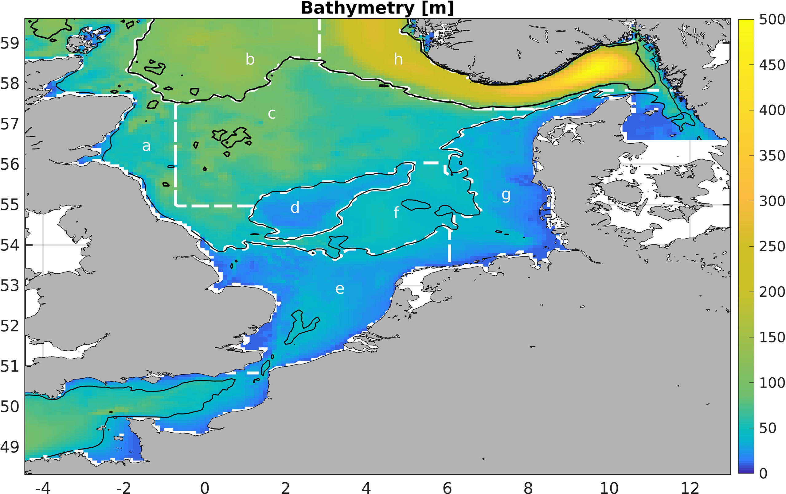
Figure 1 Model bathymetry. The thin and thick black contour lines are the 40m and 100m isobaths, respectively. The white dashed lines define the boxes over which we average (see Section Methods of Analysis).

2.2 Biological Model

The biological component of our model was the Carbon, Silicon and Nitrogen Ecosystem (CoSiNE) model, developed by Chai et al. (2002) and amended by Xiu and Chai (2011) and Liu et al. (2018). We use a version with 11 state variables, specifically four nutrients (NO₃, NH₄, SiOH₄ and PO₄), two groups of phytoplankton [small phytoplankton (P1) and diatoms (P2)], two groups of zooplankton [micro- (Z1) and mesozooplankton (Z2)], detrital nitrogen (dN) and silicate (dS) and oxygen.

The growth rate of phytoplankton is dependent on nutrient availability. For instance, the nitrate uptake for small phytoplankton is

$\begin{array}{ll}\begin{array}{cc}NPSI={\mu }_{1,\max }& ·\stackrel{I}{\overbrace{\min (uNO{3}_1+uNH{4}_1,uPO{4}_1)}}·\\ & \frac{uNO{3}_1}{uNO{3}_1+uNH{4}_1}·P_1·P1,\end{array}& \text{(2.2.1)}\end{array}$

where μ_1,max is the maximum growth rate, uNO3, uNH4 and uPO4 are the uptake rate of nitrate, ammonium and phosphate, respectively (bounded between 0 and 1), and P₁ is the photosynthetic rate for P1. Thus, if any nutrient is unavailable, growth is inhibited, due to the term marked “I”. For P2, it also includes uptake of SiOH₄. The term has a lower limit of 0 and an upper limit of 1.

P₁ is a function of irradiance:

$\begin{array}{ll}{P}_1=\left(1-\exp \left(-I\left(z\right).{\alpha }_1/{\mu }_1\right)\right)·\exp \left(-I\left(z\right)/\left({\mu }_1{\beta }_1\right)\right)& \text{(2.2.2)}\end{array}$

where α₁ is the slope of the P–I curve and β₁ is the slope for photo-inhibition. Irradiance is itself a function of depth, i.e.,

$\begin{array}{ll}I(z)=I_0·\exp (-k_{w}z-k_P{\int }_z^{\zeta }(P1+P2)d{z}^{\text{'}}-k_{SPM}{\int }_z^{\zeta }SPMd{z}^{\text{'}}).& \text{(2.2.3)}\end{array}$

Here, k_w, k_p and k_SPM are the attenuation coefficients for pure water, phytoplankton and SPM, respectively, and ζ is the sea surface. The P–I curve has a maximum, which can be prescribed at realistic values for either species. Both small phytoplankton and diatoms have a maximum growth rate between 60Wm⁻² and 100Wm⁻².

Phytoplankton growth is modulated by temperature via the Q₁₀ term, which describes the relative change in the growth rate for a temperature increase of 10K,

$\begin{array}{ll}{Q}_{10}=\exp \left(0.03·\left(T-10K\right)\right)& \text{(2.2.4)}\end{array}$

All parameters used in this study are shown in Table 1. Figure 2 shows both the Q₁₀ term and the P–I curves for both phytoplankton groups. It also shows the averages of sea surface temperature (SST) and short-wave radiation (SWR) for 1950, 2000 and the three different RCP scenarios in 2050, for the months March to May, as well as the annual SST means for the same time periods. This illustrates how changes in SST and SWR may affect plankton growth. Increases in temperature will lead to accelerated primary production, while increases in SWR due to climate change will likely not have a dramatic effect.

TABLE 1

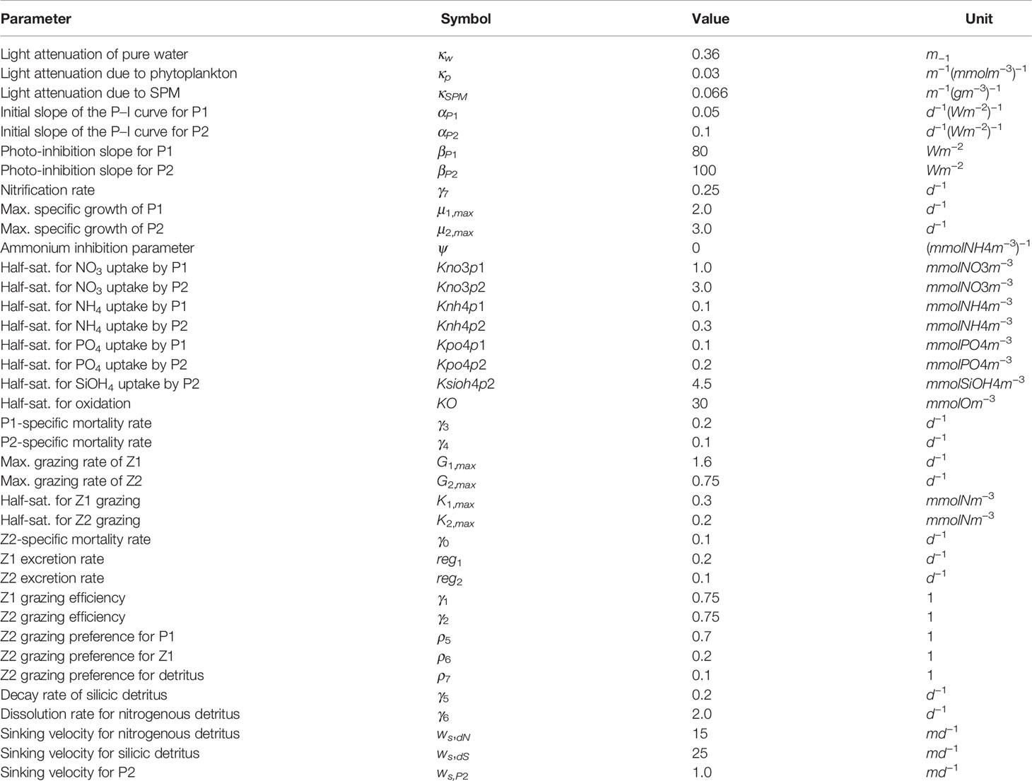
Table 1 CoSiNE parameters.

FIGURE 2

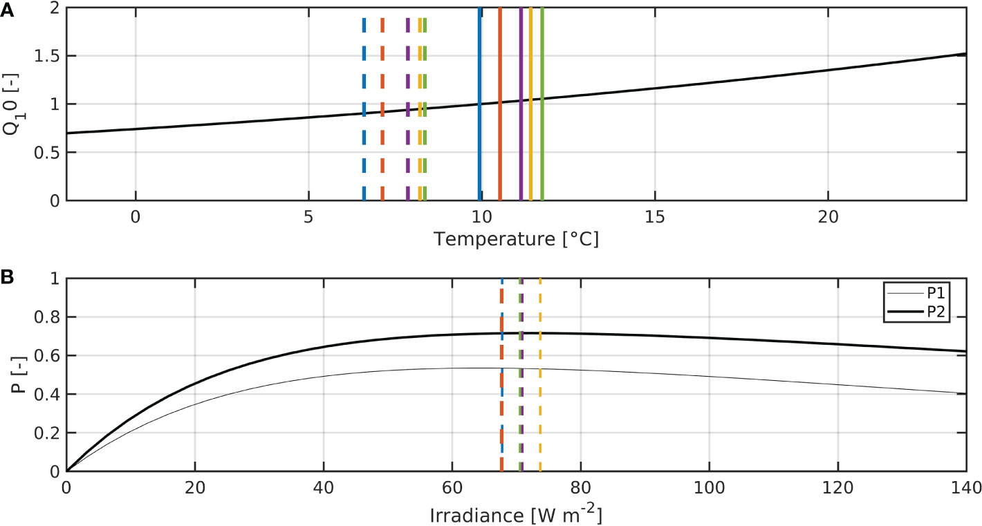
Figure 2 (A) Q₁₀-term. Dashed vertical lines show mean temperatures for March to May 1950–1954 (blue), 2000–2004 (red) and 2050–2054 (yellow: RCP2.6-SSP1, purple: RCP4.5-SSP2, green: RCP8.5-SSP5), and solid ones show the means of the 5-year period. (B) P–I curves for P1 (thin) and P2 (thick). Dashed vertical lines are the same as in the top panel, except that they show SWR averages.

At the oceanic boundaries, the nutrients are introduced via the same type of BC as temperature and salinity [radiation with nudging (Orlanski, 1976; Marchesiello et al., 2001)]. The remaining biological tracers are treated with a radiation boundary, i.e., without external forcing. River forcing is provided for all four nutrients. The ICs are derived the same way as the physical ones (see Section Physical Model), repeating the first year’s forcing five times. The differences between the fourth and fifth iterations were at the level of machine precision.

2.3 Used Data

The setup used in this study is derived from those used in Thewes et al. (2020) and Thewes et al. (2021). It differs, however, with respect to the applied boundary forcing, as the previously used data sets do not cover all periods of interest, specifically the periods of 1950–1954, for most of the data, as well as any period in the future. The updated oceanic and atmospheric model forcing was taken from the Max Planck Institute for Meteorology’s (MPI-M) Earth System Model 1.2 with high resolution (MPI-ESM1-2-HR) (Gutjahr et al., 2019), performed by Deutsches Klimarechenzentrum (DKRZ) in Hamburg, Germany. The nominal resolution for the atmosphere is 100 km, and 50 km for the ocean physics and biogeochemistry. The data were generated in the context of the internationally coordinated Coupled Model Intercomparison Project Phase 6 (CMIP6) (Eyring et al., 2016). The scenarios used were the historical run (Jungclaus et al., 2019) for the runs starting in 1950 and 2000, RCP2.6 with SSP1 (Schupfner et al., 2019a), RCP4.5 with SSP2 (Schupfner et al., 2019b) and RCP5.8 with SSP5 (Schupfner et al., 2019c).

The river forcing was also changed with respect to the previous publications. We now use a composite data set, comprising data from the pan-European Hydrological Predictions for the Environment model (E-HYPE) of the Swedish Meteorological and Hydrological Institute (SMHI) for rivers and Fjords in Sweden and Norway, as well as the Intersessional Correspondence Group on Eutrophication Modelling (ICG-EMO) data set by the Oslo and Paris (OSPAR) Commission (Lenhart et al., 2010). The data from E-HYPE are climatological for the years 2000–2004 and provides forcing for rivers and fjords in Sweden and Norway, while that from the ICG-EMO is a mixture of observational, modelled and climatological data at a daily frequency. It is used for rivers from all other countries neighbouring the North Sea. Particularly for the period of 1950–1954, the ICG-EMO data are mostly climatological.

The SPM data used to force the model are provided by IFREMER (2017). Descriptions of the algorithm to determine the SPM concentration from ocean colour are found in Gohin et al. (2005) and Gohin (2011). The method by which it is introduced to ROMS-CoSiNE is described in Thewes et al. (2021).

For validation purposes, we used data from the E.U. Copernicus Marine Service Information, specifically the Global Reanalysis data set CMEMS-GLO-PUM-001-030. Bottle data of nutrients and chlorophyll were provided by the International Council for the Exploration of the Seas (ICES). Satellite-derived chlorophyll data were provided by the Ocean Colour Climate Change Initiative (OC-CCI), of the European Space Agency at version 4.1.

2.4 Experiment Design

A prediction of the future North Sea light climate has—to our knowledge—never been attempted with a numerical model. We thus had very little experience or previous research to rely or build on. A set of runs was performed using climatological monthly means of satellite-derived SPM (IFREMER, 2017) from the years 1998 to 2017 and, in the case of the runs that start in the year 2050, using the same river forcing as in that starting in 2000. The only variant factor in downwelling attenuation in these runs thus is that which is due to phytoplankton. Going forward, we will refer to these five runs as base runs. They are referred to as r1950, r2000, r2050_1 (RCP2.6-SSP1), r2050_2 (RCP4.5-SSP2) and r2050_3 (RCP8.5-SSP5). They serve the purpose of a control and reference to the SPM increase experiment. All runs have the same duration of 5 years. As described above, all initial conditions were spun up by applying the forcing of the first year five times before the actual run.

In Thewes et al. (2021), two different sets of satellite-derived SPM (the same IFREMER data set, as well as one provided by GlobColour at www.globcolour.info) were used to provide sediment-specific attenuation to the model, and linear trends in SPM were calculated. For the IFREMER data, these revealed that over the period of 1998–2017, SPM concentrations may have increased in several regions of the North Sea. The strongest increases that were found to be statistically significant were in orders of 6% annually, with a basin-wide average of about 0.8%y⁻¹. The other data set (GlobColour) showed weaker increases, as well as decreases elsewhere. For a discussion of these results, the reader is referred to Thewes et al. (2021). Generally, it is inadvisable to extrapolate such trends decades into the future, as trends need not be linear in the long term. However, because the state of knowledge of SPM concentrations in the future North Sea is still incomplete, we nevertheless made the assumption that there really was an overall increase of SPM by 0.8%y⁻¹ over the period of 2000–2017, which continues until 2050. On the basis of this, we conducted a modelling case study, in which we increase the climatological SPM by 40% everywhere, in correspondence to the 0.8%y⁻¹ increase found in Thewes et al. (2021), applied over 50 years. We discuss the implications and uncertainties of this approach in Section Model Uncertainties and Limitations. The runs that were performed in the context of these experiments are identified by the tag “SPMp40” behind its corresponding base run’s identifier. A summary of all runs we performed in this work is found in Table 2, which lists the name identifiers given to them, all forcing applied to them and their respective time periods.

TABLE 2

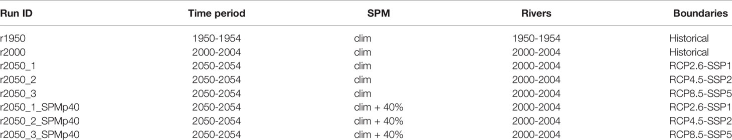
Table 2 Summary of all runs. “clim” refers to monthly climatological means for the period of 1998–2017.

The choice of time periods is based on several considerations. For one, there is data availability. We would have preferred to perform a run starting in 1900, but due to a lack of reliable data, we instead chose the period of 1950–1954 for a historic scenario. Furthermore, assumptions made on the development of SPM content are baseless without supporting data. There are studies which focus on the development of the wind wave regime (Casas-Prat et al., 2018), which may serve as a reference. However, to our knowledge, there are now sources of SPM for the period of interest, 2050–2054 specifically. It is also well known that the North Sea ecosystem has undergone shifts in the past (e.g., Radach, 1998; Wiltshire et al., 2008), with progressing eutrophication in the 1970s up to the mid-1980s. It is thus not advisable to choose too large time spans between runs. By our choice of time periods, we circumvent the period of eutrophication, which might perhaps have made interpretation of our results more challenging. We thus have one pre-eutrophic and one post-eutrophic historic run, respectively, and three future scenario experiments. It is important to understand that a linear development between the time slices must not be inferred.

2.5 Methods of Analysis

We calculated the depths at which the irradiance has 10% of the surface level, i.e., the 10% depth, or Z₁₀, which is a measure for water clarity. Furthermore, we computed the biomass that is above Z₁₀, which is

$\begin{array}{ll}{P}_{10}={\displaystyle {\int }_{z_{10}}^{\zeta }\left(P1+P2\right)dz}& \text{(2.5.1)}\end{array}$

where ζ is the sea surface, and P1 and P2 are small phytoplankton and diatoms, respectively.

To filter out the effects of horizontal meso- and small-scale variability, we perform area averages of Z₁₀, P₁₀, SST, SWR and oceanic nutrients over specific regions, which are shown in Figure 1. The area averages are denoted by

$\begin{array}{ll}\langle X\rangle =\frac{1}{A}{\displaystyle {\int }_A\chi }dA& \text{(2.5.2)}\end{array}$

where χ is the respective quantity and A is the area. The areas’ names are north-western North Sea (a), central North Sea (b), northern North Sea (c), Dogger Bank (d), southern North Sea (e), Oyster Grounds (f), eastern North Sea (g) and Norwegian Trench (h). All boxes have a relatively homogeneous depth.

For all 5-year runs, we computed daily climatological means, i.e., averages over each day of the year for the entire 5-year period, of all area averages. All variables we investigate have a strong seasonality. Therefore, they are not normally distributed and thus harder to compare statistically. By subtracting daily climatologies from the area averages, we arrive at residuals, which are normally distributed. For the base runs, we chose r2000 as the reference and subtracted its daily climatologies <χ_r2000>_dc from the area averages of all base runs. Note that, strictly speaking, this no longer gives residuals per se, but rather a type of biased anomaly; however, for reasons of better readability, we will continue using the term residuals, even when we refer to quantities that are derived from comparing two different runs. Residuals will be marked by the subscript letter r, e.g., <χ>_r. By applying a two-variable t-test, we determined whether changes in the 5-year averaged residuals relative to r2000 in case of the base runs, and relative to the respective base run for the SPMp40 runs, are statistically significant. The null hypothesis of the t-test was that the 5-year means of the residuals have not significantly changed. Note also that when we speak of significant changes, it typically refers to statistical significance only.

Because the natural ranges of NO₃ and PO₄ in the North Sea differ by two to three orders of magnitude, we normalized their residuals by the 5-year means of the area averages μ for the run r2000, yielding a relative quantity. The normalized quantities will be marked by the letter n in the index:

$\begin{array}{ll}{\langle \chi \rangle }_{rn}=\frac{\langle {\chi }_i\rangle {}_r-{\langle \chi r2000\rangle }_{dc}}{{\mu }_{\langle \chi r2000\rangle }}& \text{(2.5.3)}\end{array}$

3 Results

3.1 Base Runs

For reference, the daily climatologies of <Z₁₀>, <P₁₀>, <SST>, <SWR>, <NO3>, and <PO4> are shown in Figure 3. There is clear seasonality in all of the variables. The deepest <Z₁₀> are found in the deepest areas (a–c and h) in September. In the other areas, <Z₁₀> is shallower than 20m for most of the year. <P₁₀> is the aggregate depth-integrated and area-averaged biomass of P1 and P2 above Z₁₀. The leading peak is the diatom (P2) spring bloom. The trail of <P₁₀> is mostly consistent of small phytoplankton (P1). For the nutrients, the seasonality is weaker than the spatial variability. The highest nutrient levels are found in the eastern North Sea (g).

FIGURE 3

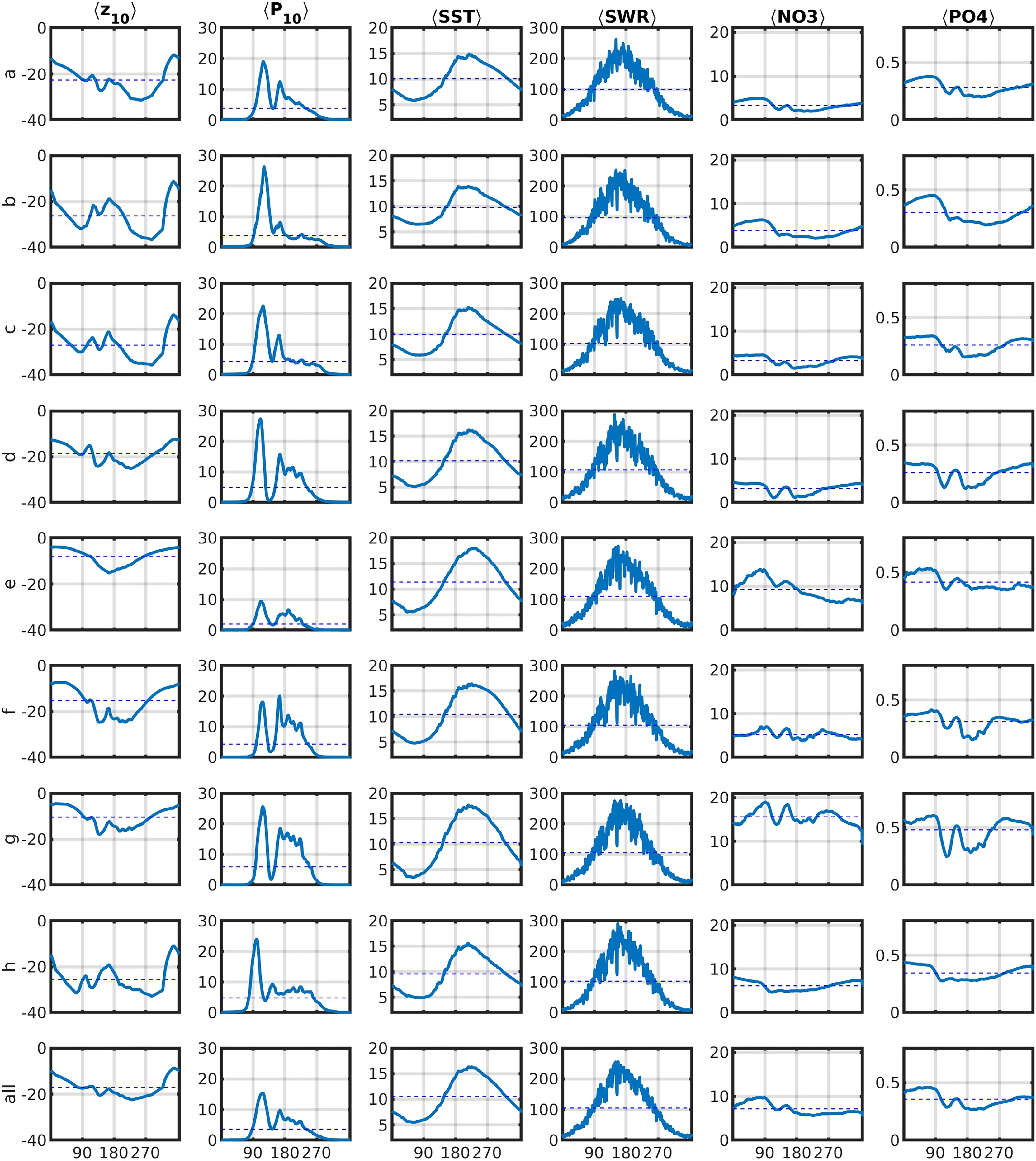
Figure 3 Daily climatologies of <Z₁₀> [m], <P₁₀> [mmolNm^-3], <SST> [ C], <SWR> [Wm^-2], <NO3> [mmolNm^-3] and <PO4> [mmolNm^-3] of all areas (see Figure 1) for r2000. Dashed lines denote 5-year means.

Figure 4 shows the daily climatologies of <P1₁₀> and <P2₁₀>. It becomes evident that for all future runs, biomass for both phytoplankton groups is significantly lower overall, compared to r2000. The diatom spring bloom occurs later in the year for areas a, b, c and d, while that for small phytoplankton occurs at roughly the same time, but with much lower magnitude. Areas e–h show smaller differences in timing and magnitude of the diatom spring bloom. In areas e and g, it starts slightly earlier in the 2050 runs than in r2000 or r1950, which is likely a consequence of temperature increase. For most areas, the curves of <P2₁₀> are of significantly lower magnitude in all future runs. Relative to r2000, r1950 often shows similar or higher magnitudes of<P1₁₀> and <P2₁₀>.

FIGURE 4

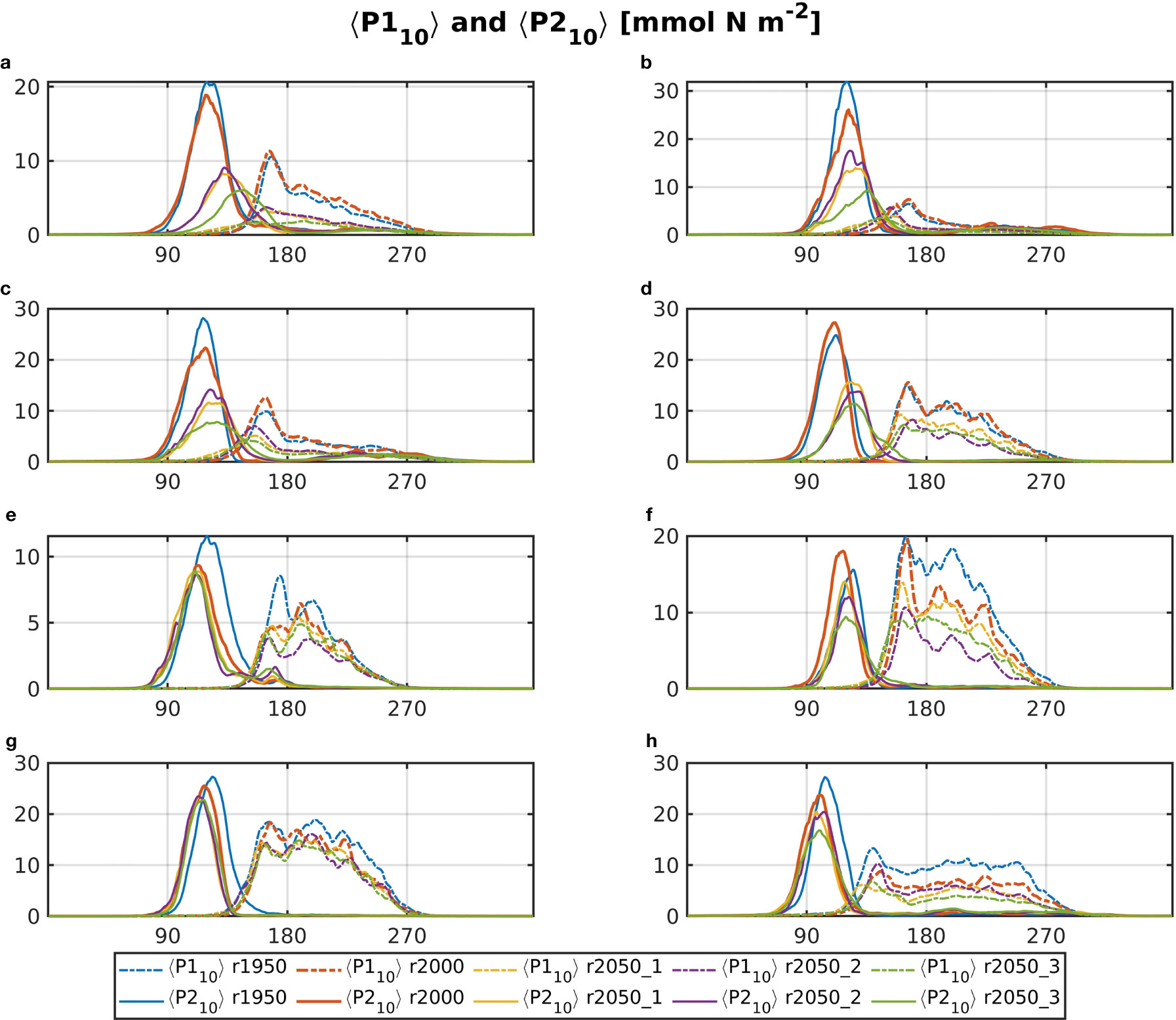
Figure 4 Daily climatology of <P1>₁₀ (dotted dashed) and <P2>₁₀ (solid) for all base runs (blue: r1950, red: r2000, yellow: r2050_1, purple: r2050_2, green: r2050_3). The letter tags in the panel’s titles refer to the areas, which are shown in Figure 1.

The daily climatological means of <Z₁₀> for all base runs and all areas are shown in Figure 5. There is a semiannual cycle in <Z₁₀> in boxes a to c and h, which is caused by a summer maximum in SPM. As explained in Section Experiment Design, changes in Z₁₀ between runs are solely due to differences in phytoplankton for all base runs. Thus, it is unsurprising that the greatest differences between the runs occur in the second quarter of the year, at the time of the spring bloom. The impacts of reduced phytoplankton biomass on <Z₁₀> are most apparent for r2050_3 in the north-western areas, where for areas a–c a spring bloom-related event of shallower <Z₁₀> is almost entirely absent, whereas it is at least somewhat noticeable for the other future runs. As is seen in Figure 4, the diatom bloom occurs weeks later and much lower in r2050_3 for those areas.

FIGURE 5

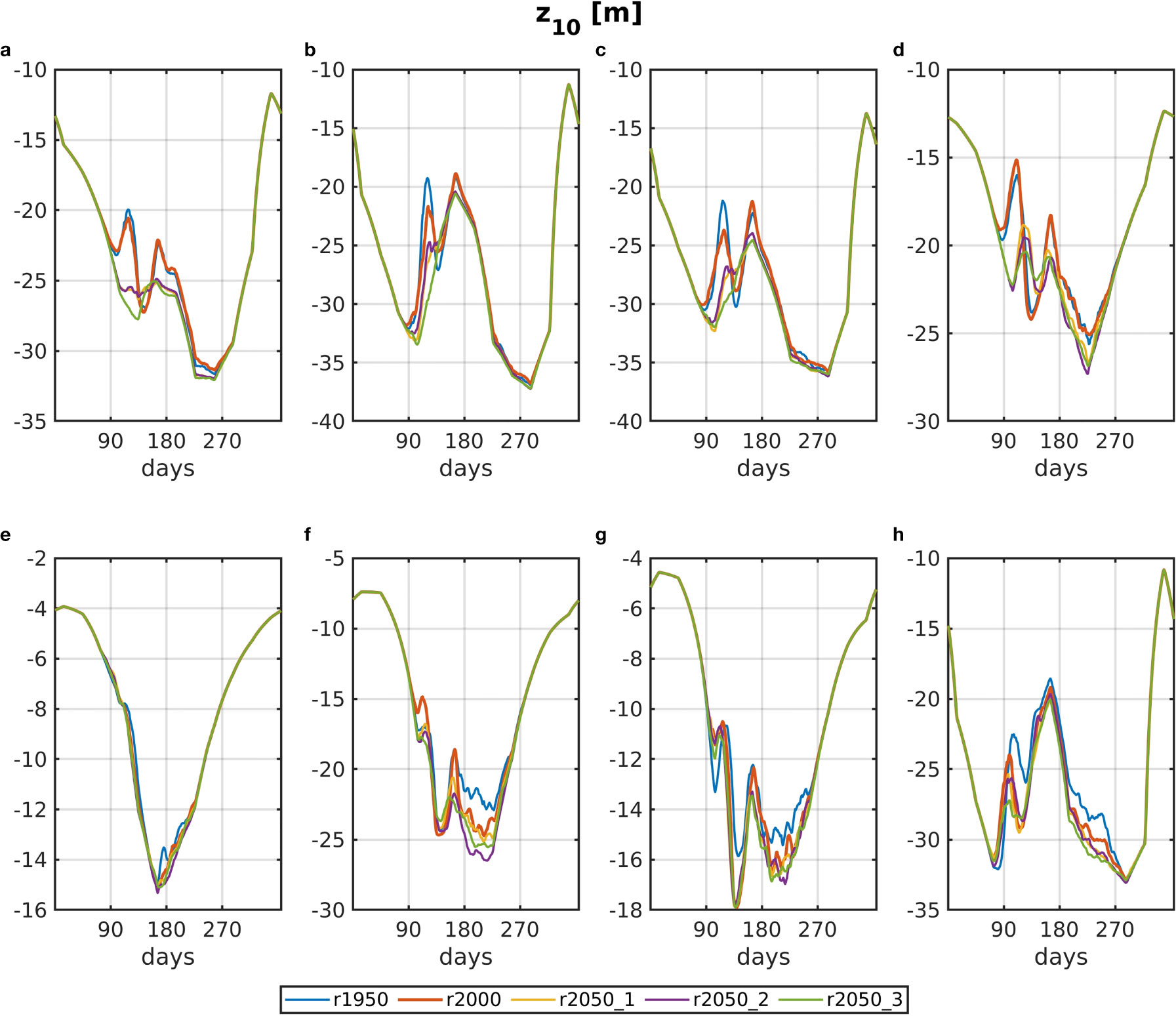
Figure 5 Daily climatology of <Z>₁₀ for all base runs (blue: r1950, red: r2000, yellow: r2050_1, purple: r2050_2, green: r2050_3). The letter tags in the panel’s titles refer to the areas, which are shown in Figure 1.

For r1950, the results of the t-test for all tested variables were positive, i.e., statistically significant for all areas, except areas b, c and d, which are highly dominated by oceanic inflow. Due to the different river forcing, the greatest differences between r1950 and r2000 for <Z₁₀>_r, <P₁₀>_r, <NO3>_rn and <PO4>_rn are found in the areas where the largest rivers discharge into the North Sea, and the adjacent Oyster Grounds (e–h, Figure 6). There, particularly, nitrate levels were much lower in r1950 than they were in r2000, while phosphate levels were considerably higher. The greatest difference in <Z₁₀>_r between r1950 and r2000 is found at the Norwegian Trench (h), where for r1950, <Z₁₀> is shallower than for r2000 by (0.61 ± 1.77)m. This may be attributed to the effects of eutrophication, which occurred between the periods of 1950–1954 and 2000–2004, caused by increased river nutrient inflow. Also, since the area is the deepest on average, it experiences lower SPM influence than the southern regions of the North Sea, so that the reference value of <Z₁₀> is relatively large. The changes in <Z₁₀>_r are thus relatively smaller.

FIGURE 6

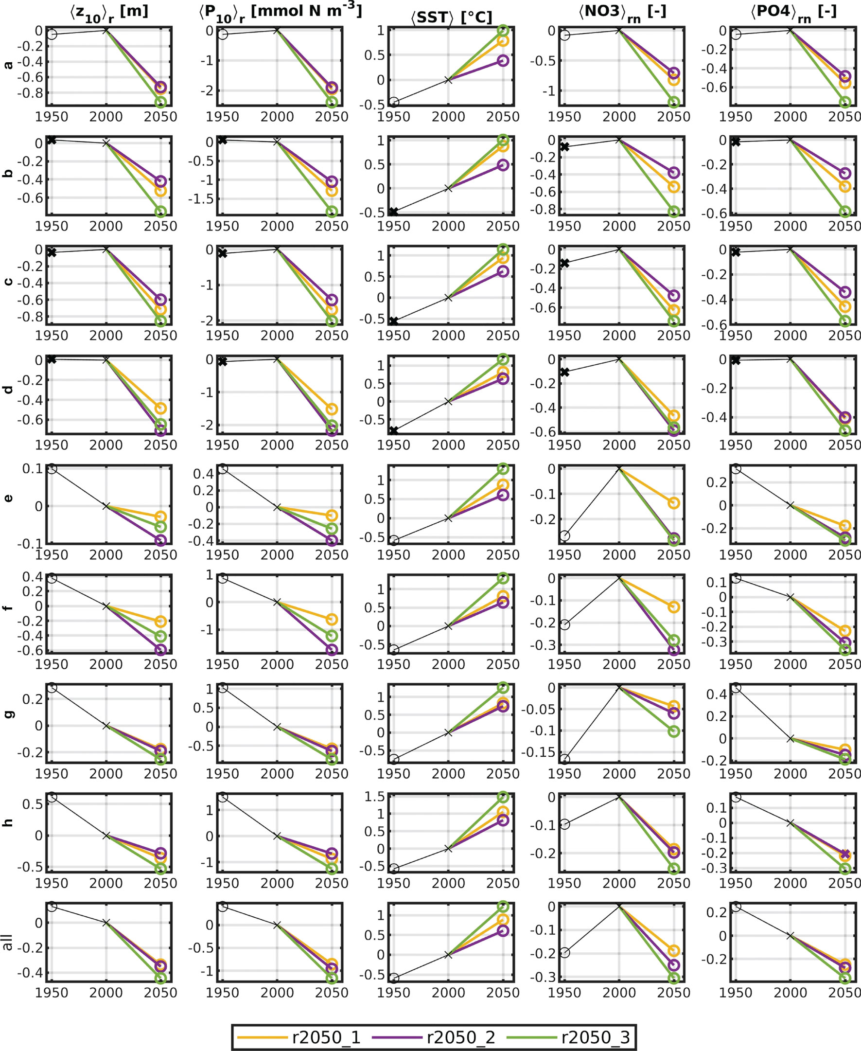
Figure 6 Five-year means of <Z₁₀>_r, <P₁₀>_r, <SST>_r, <NO3>_rn and <PO4>_rn. (column order) for all areas (row order) and all base runs. NO₃ and PO₄ are normalized by the respective 5-year means of r2000. The results of the t-test are marked with circles (significant change) and crosses (insignificant change) for all runs except r2000.

The deviations for the future runs are in any case significant. The 5-year means of <Z₁₀>_r, <P₁₀>_r, <SST>_r, <NO3>_rn and <PO4>_rn are shown in Figure 6 (note that NO₃ and PO₄ are normalized, as explained in Section Methods of Analysis, to give an estimate of relative change). For all areas, it is obvious that <P₁₀> almost linearly affects <Z₁₀>.

It is also apparent that r2050_1, despite being the “optimistic” scenario, has consistently higher <SST>_r than r2050_2 (see also above and Figure A.3 in the appendix). It is generally noteworthy that the means for r2050_1 are consistently above or below (depending on the respective variable) those for r2050_3, yet those for r2050_2 are sometimes higher than both, lower than both or in between. The influence of temperature on the magnitude of the 5-year averaged <P₁₀> appears to be negligible for the most part.

All future runs show significantly lower values for the 5-year averaged <P₁₀>. The driving factor for this is nutrient availability. For areas a, b, c and d, nitrate and phosphate are at similar levels in 1950 and 2000, yet much lower, at similar proportionality to <P₁₀> levels, in 2050. The levels are lowest in r2050_3 in every area, except the Oyster Ground (f), where r2050_2 is lowest in nitrate. r2050_1 consistently has higher nutrient levels than r2050_3. The levels of r2050_2 are higher than r2050_1 in areas a–c, and lower or the same everywhere else. For <Z₁₀>_r and <P₁₀>_r, this is the case as well, except for areas g and h (eastern North Sea and Norwegian Trench). Here, the 5-year means of the residuals for all variables in r2050_1 and r2050_2 lie closely together. Because Z₁₀ is a negative quantity, a decrease corresponds to increased water clarity. The deepening of <Z₁₀> is never more than 1m and highest in the deeper regions in the north-west of the North Sea (a–c).

Figure 7 shows the limiting nutrients for both phytoplankton groups against time (see Section Biological Model and Equation 2.2.1, term “I”). Note that the term “limiting” is used here simply to identify the nutrient which is least available, thus limiting the growth, although the overall growth rate need not be small. Figure 7 thus shows simply which nutrient is least available. Phytoplankton growth is limited by either nitrogen (NO₃ or NH₄), or phosphate uptake (diatoms theoretically could be limited by SiOH₄; however, this was never the case in any of our runs). It shows that for diatoms (P2), the north-western boxes (a–d) are predominantly limited by nitrogen, and the southern boxes are mostly limited by phosphate. r1950 shows nitrogen limitation for diatoms in all areas, which is overtaken by phosphate limitation in spring, effectively ending the diatom spring bloom (compare Figure 4). This is also the case in the north-western areas a–d for r2000, yet not for the southern areas or the Norwegian Trench, which is due to relatively higher nitrogen input from rivers. Small phytoplankton (P1) is predominantly limited by phosphate. The 2050 runs are not limited by phosphate in areas a–c. The low magnitudes of diatom blooms in those regions are thus explained by low nitrate levels (see also 4 and 6). At the Dogger Bank (d), there is a transition, where for all runs the diatom bloom is terminated by phosphate limitation. Conversely, for P1, areas a and b show nitrogen instead of phosphate limitation for the future runs.

FIGURE 7

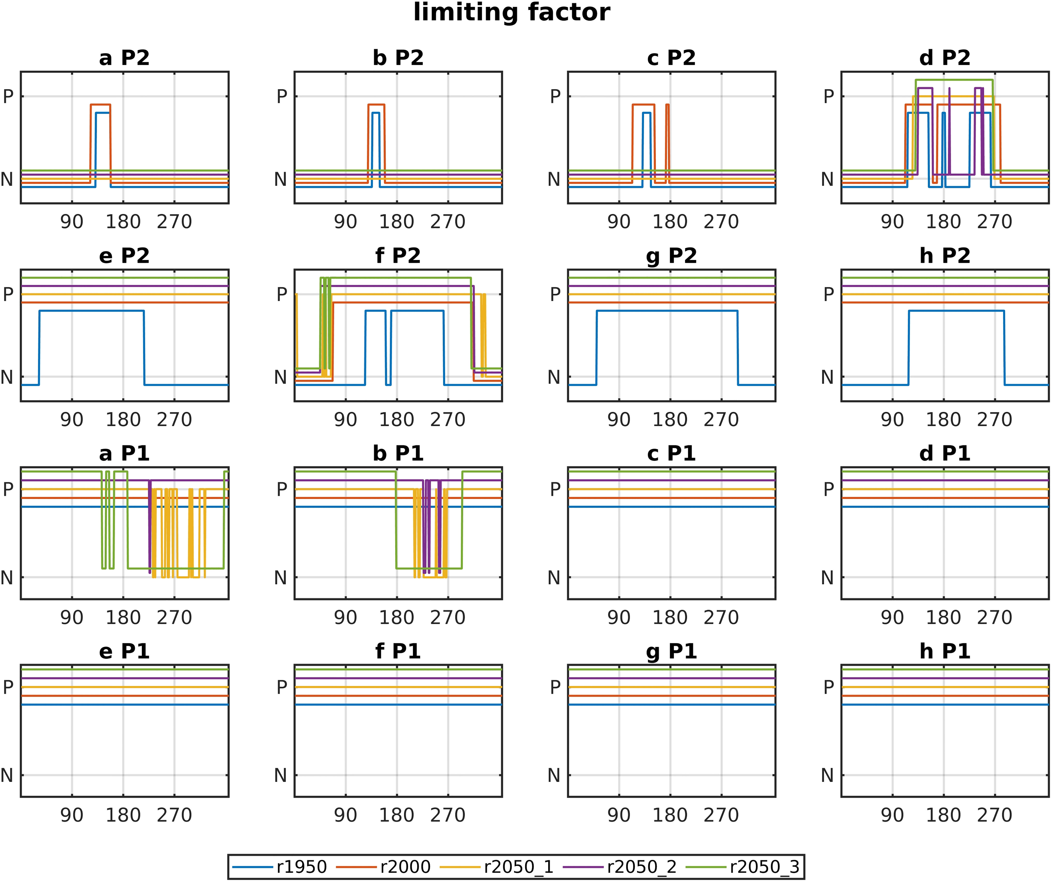
Figure 7 Nutrient limitation of phosphate and nitrate or ammonium (see Section Biological Model and Equation 2.2.1) for all base runs and areas against time. The top two rows are diatoms and the bottom two rows are small phytoplankton.

3.2 SPM Changes

Raising the SPM monthly climatology linearly by 40% led to decreases in 5-year averaged <Z₁₀> ranging from (1.9 ± 0.67)m (r2050_1_SPMp40, (23 ± 8)% relative to the respective base run) in the southern North Sea (e), to (4.6 ± 1.15)m (r2050_3_SPMp40, (16 ± 2)%, Figure 8A) in the central North Sea (c). Over all areas, the average decrease is (3.2 ± 0.6)m in all future runs. This makes for approximate relative changes of (15 ± 3)%, compared to the respective base runs. The deeper areas (a–c and h) showed larger shifts, which is due to generally lower levels of <Z₁₀> (compare Figure 3), as a decrease by 1m requires lower increases in down-welling attenuation when the 10% depth is 30m than when it is 10m (Dupont and Aksnes, 2013; Lee et al., 2015). Phytoplankton biomass was lower, compared to the base run (Figure 8B). The reductions were found to be statistically significant, but at low magnitudes, compared to the reductions caused by nutrient limitation in the base runs for 2050, relative to r2000.

FIGURE 8

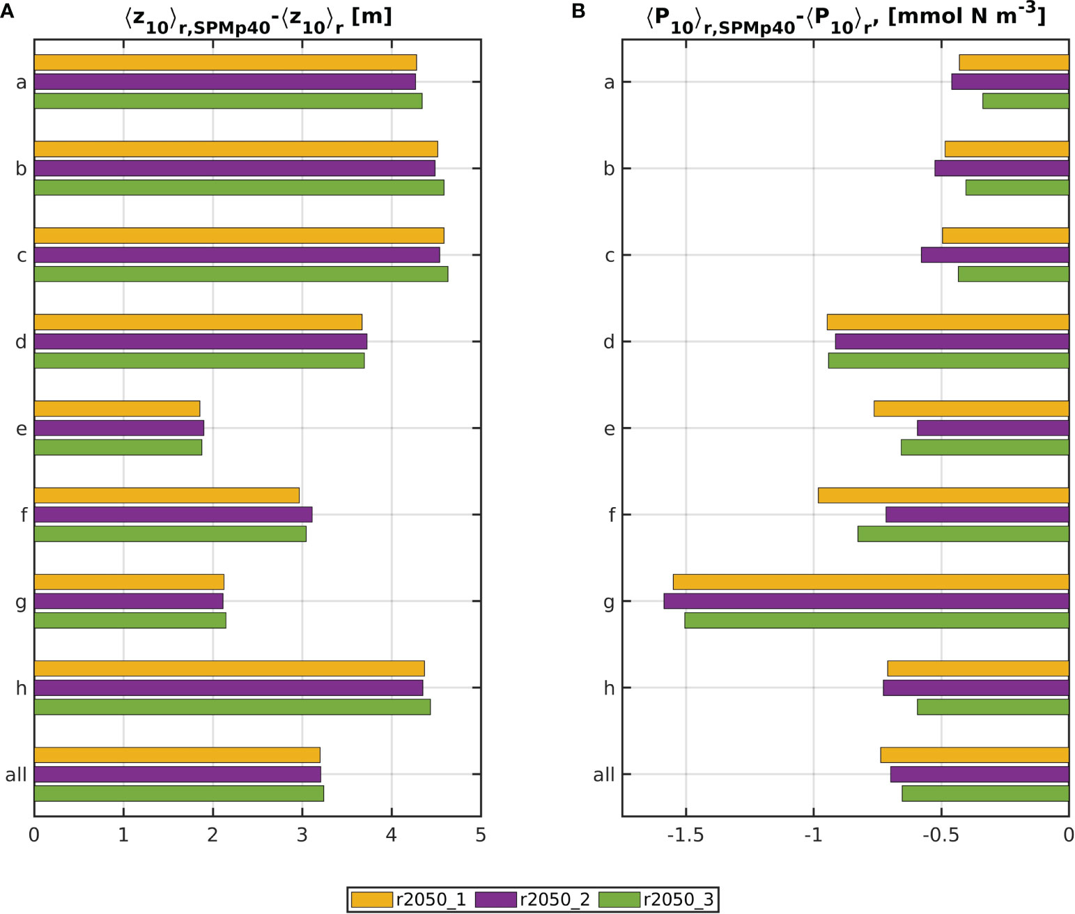
Figure 8 Differences in 5-year means of <Z₁₀>_r and <P₁₀>_r between the SPMp40 runs and the base runs. Yellow is r2050_1, purple is r2050_2 and green is r2050_3.

Similarly to the base run experiments, where the 5-year means of residual area averages for r2050_2 did not sit consistently between those for r2050_1 and r2050_3, the deviations of <Z₁₀> and <P₁₀> in r2050_2_SPMp40 are sometimes higher and sometimes lower than those in the two other 2050 SPMp40 runs. For areas d, e and f, <P₁₀> reductions are lower than those of the other runs, and for the remaining areas, they are higher. Consequently, the reverse is the case for <Z₁₀> increases. Only when averaging over all areas do the deviations in r2050_2_SPMp40 sit between those of r2050_1_SPMp40 and r2050_3_SPMp40. When comparing Figures 6 and 8, it becomes apparent that this is because of nutrient availability: in areas a to c, both <NO3> levels were higher, and <P₁₀> reductions due to SPM were stronger in r2050_2_SPMp40 than in the other two SPMp40 runs. In areas d–f, the opposite is true. In the eastern North Sea (g) and the Norwegian Trench (h), nitrate levels are slightly lower in RCP4.5-SSP2 than in RCP2.6-SSP1, but reductions caused by the SPM increase are higher in r2050_2_SPMp40. Yet the respective 5-year means are very close to each other.

4 Discussion

4.1 (I) How Does Phytoplankton Growth Change Under Future Climate Conditions?

All future base runs showed significant decreases in biomass. This is due to lower nutrient levels. Both nitrate and phosphate are projected to decline. The entire reason for this decline is lower nutrient influx at the horizontal boundaries, as the river forcing is the same between r2000 and the future scenarios. While in areas e–h the nitrate levels in 2050 sink to levels similar to those in 1950, phosphate levels in 2000 were already lower than those in 1950, and they further decreased for 2050. For areas a–d, levels of both phosphate and nitrate are substantially lower in 2050 than they are in the historic scenarios, for which they are about the same everywhere. Reductions in surface nutrients have been predicted in earlier studies concerning the North Sea ecosystem in the 21st century, attributed to stronger stratification in the open ocean. This would then cause lower on-shelf nutrient transport and lower primary production (Holt et al., 2012). In fact, at all open boundaries, the levels of NO₃ and PO₄ concentrations in all 2050 scenarios were significantly lower than in 2000 (up to 50%). Further nutrient reductions, due to the efforts made to reduce fluvial nutrient loads, are likely, but challenging to predict (as discussed later this section). The effects of changing SST and SWR on phytoplankton growth appear insignificant compared to those of nutrient limitation.

It needs to be noted that a decrease in biomass need not exclusively be a bad thing, per se. Our model is not designed for studies on eutrophication, although it has been applied in similar ways (Zhou et al., 2017). See Section Model Uncertainties and Limitations for a discussion of the applicability of the model. Given that it is the expressed goal of the OSPAR convention to eliminate eutrophication, our results suggest a positive development; however, this can mostly be said for the northern North Sea and is not to be taken at face value. The dominant driver of nutrient levels in the southern North Sea is riverine inflow, which we have assumed to be at the same levels as around 2000–2004. We therefore cannot draw any conclusions on the development of eutrophication in the North Sea.

Using a model developed by Cole and Cloern (1987), Capuzzo et al. (2018) computed long-term trends of phytoplankton biomass for the time period of 1988 to 2013, finding significant decreases for regions they called transitional west and transitional east (these largely fall into the areas a, f and g in this study; see their Figure 1), as well as over the whole domain, attributing this to temperature increases and reductions in river nutrients. In our model, river nutrients are the same in r2000 and all future runs. Consequently, the biomass decreases for the future runs are smallest in areas e, g and h, which are those with the highest input of river nutrients. If the efforts made to reduce fluvial nutrient loads are successful, the decreases in biomass are likely to be much greater than in our future projection. A sensitivity study with focus on nutrient loads would help to clarify this; however, the challenges involved in this are substantial and require care and rigor. Even for present-day scenarios, river forcing remains a challenge (Lenhart et al., 2010). Furthermore, as described by Stegert et al. (2021), it is difficult to define what a pre-eutrophic state of the North Sea is. To achieve such a state may even be impossible. Thus, realistic targets need to be defined. In the context of the water framework directive (WFD) and the marine strategy framework directive (MSFD), set by the European Union, target values for nutrient levels are defined, which may give a reasonable starting point []? (see, e.g., Phillips et al., 2018, Poikane et al., 2019). Going by the strategy of the SSP, one might define pathways specifically for river forcing. However, the combined workload may well require multiple papers to cover. Furthermore, the regions in our model that showed the largest reductions in biomass (a–d) are the ones that are most sensitive to nutrient inflow from the Atlantic. Capuzzo et al. (2018) studied a time period different from ours. In context of each other, their work and ours support the hypothesis that biomass in the North Sea will likely decrease significantly.

For all future runs, and particularly for r2050_3, there were obvious shifts in timing of phytoplankton blooms (Figure 4), which are in most cases due to nutrient limitation, causing a delay by several weeks, compared to r2000. In the areas of highest river run-off, (e, g and h, respectively), there was no such delay, but rather a forward shift by several days. This is likely due to increased temperatures (Equation 2.2.4). However, we will not go into greater detail here, as we neglect other effects of increasing temperature, such as higher zooplankton activity (Wiltshire et al., 2008).

4.2 (II) How Does Varying SPM Impact the Development of the Ecosystem?

The raising of SPM by 40% caused a shallowing of Z₁₀, as was to be expected. The decrease in magnitude was nearly 20%, which was up to an order of magnitude higher than the deepening of <Z₁₀> that was found for the base runs, due to reductions in biomass. Biomass is generally assumed to be a less significant contributor to light attenuation than SPM or CDOM (e.g., Dupont and Aksnes, 2013; Capuzzo et al., 2015; Opdal et al., 2019).

Changes in biomass due to the lower light availability were found to be statistically significant; however, in terms of magnitude, they were small compared to the effects of nutrient limitation. The SPMp40 runs showed reductions in biomass in orders of 1%−2%, relative to the respective 2050 base runs, which is an order of magnitude lower than those reductions found for the future runs, relative to r2000 (see 4.1).

All future scenarios were very close to each other in terms of Z₁₀ and P₁₀ change due to increased SPM. Typically, <Z₁₀> increases and <P₁₀>_r reductions were slightly larger in r2050_3_SPMp40 than in r2050_1_SPMp40. Changes in r2050_2_SPMp40 were sometimes greater and sometimes less than in the other two SPMp40 runs, which was found to coincide with nutrient levels.

There is a coupling between Z₁₀ and P₁₀, as stronger light attenuation (i.e., shallower Z₁₀) leads to reduced light availability, which yields lower phytoplankton productivity. This in turn provides a negative feedback on Z₁₀, as reduced phytoplankton biomass means reduced downwelling attenuation. Our results indicate that for RCP2.6-SSP1 (r2050_1), the ecosystem could be more sensitive to light limitation than for the other scenarios. Equation 2.2.1 helps to understand the principle behind this. The higher the term I is, the larger the contribution of the photosynthetic rate becomes.

As stated in Section I) How Does Phytoplankton Growth Change Under Future Climate Conditions?, we do not go into detail about timing of phytoplankton growth, as neither is it a central point of this work, nor is the model well suited for such investigations. Aside from the aforementioned missing effects of zooplankton activity (Wiltshire et al., 2008), the rate of the SPM forcing is at monthly rates only, thus too low to resolve synoptic changes and events, such as storms or periods of low wind stress. For such purposes, the application of a dedicated SPM module is preferable, due to its shorter response times and its capability to react to sudden wind changes. However, it would be negligent not to mention that the increase in SPM caused a significant shift in timing for both groups, in the orders of weeks. This was to be expected, given the higher light limitation. It has been shown that such a delay of the spring bloom can be expected in a darkening coastal ocean (Opdal et al., 2019).

4.3 (III) What Implications Do These Findings Have for the North Sea Light Climate?

A reduction of phytoplankton biomass, as projected in both the future runs and the SPMp40 runs, would yield increased water clarity. The deepening of the 10% depth due to lower phytoplankton self-shadowing would be in orders of 1%, relative to the levels of 2000.

The levels of <Z₁₀> are shallower in the southern North Sea for r1950, relative to r2000, which is entirely due to larger phytoplankton biomass. Not considering changes in SPM before the year 2000, and neglecting CDOM entirely, we cannot claim to accurately simulate a 1950 situation. Nevertheless, based on, e.g., the findings of Capuzzo et al. (e.g., Capuzzo et al., 2015), our projection is well within plausible ranges. According to Lee et al. (2015), the Secchi disk depth is the inverse of the downwelling attenuation coefficient k_D, and thus,

$\begin{array}{ll}{Z}_{SD}=Z_{10}·0.43& \text{(4.3.1)}\end{array}$

because

$\begin{array}{ll}{k}_D=Z_{10}^{-1}·\ln \left(\frac{I\left(z_{10}\right)}{I_0}\right)& \text{(4.3.2)}\end{array}$

Figure 9 shows the 5-year averaged Secchi-disk depth for r2000. We find good agreement with the measurements shown in Capuzzo et al. (Capuzzo et al., 2015, their Figure 2) for r2000. Given that Z_SD in r1950 is deeper in the orders of centimeters to decimeters, we acknowledge that the r1950 results likely are biased positively for Z₁₀ and, correspondingly, downwelling attenuation. Note that because Z₁₀ is a negative quantity, a positive bias means a shallowing of the 10% depth. Unfortunately, due to data sparsity, a direct comparison against Secchi-disk data was impossible for both r1950 and r2000. Nevertheless, it is reasonable to assume that SPM levels would have been significantly lower in 1950 than they were in the period of 1998–2017, which we use to force all of our runs (Capuzzo et al., 2015; Opdal et al., 2019).

FIGURE 9

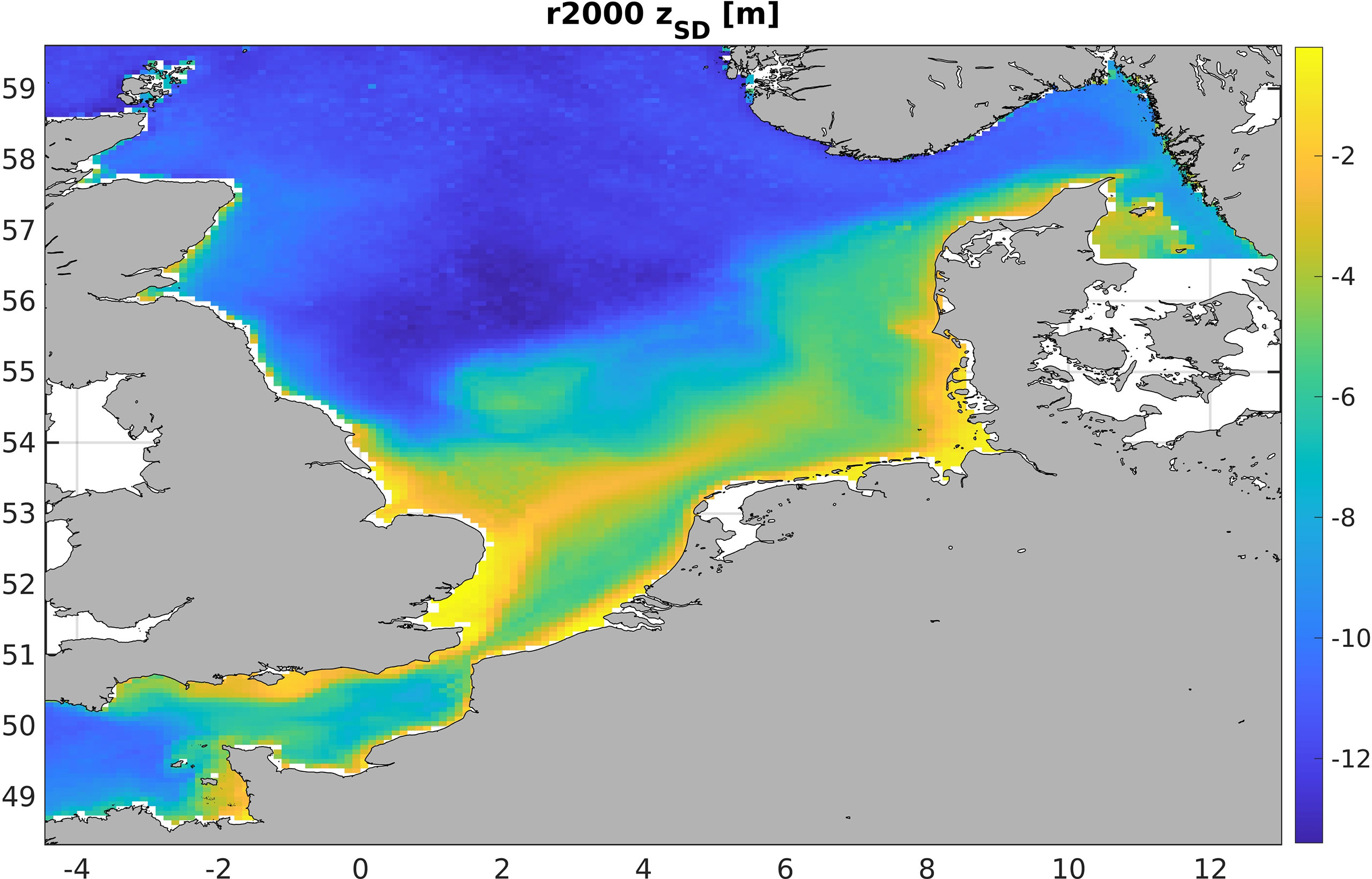
Figure 9 Five-year averaged Secchi-disk depth for r2000, calculated from z₁₀ following Equation 4.3.1.

The shallowing of <Z₁₀> due to increased SPM was found to be in orders of 20%. Thus, it is an order of magnitude larger than the deepening due to a phytoplankton biomass decrease. Although there is cause to expect SPM to increase over the coming decades, based on the current trends in SPM, this is by no means certain, and the amount by which it might is difficult to predict. Furthermore, as e.g., van der Molen et al. (2013) and Casas-Prat et al. (2018) show, the wind regime may change in such a way that SPM levels decline toward the end of the century. Note that Casas-Prat et al. (2018) analysed significant wave heights for a period of 2081–2100. Therefore, their findings may not be entirely relatable to ours. However, as Stanev et al. (2006) have shown, sea-level rise may also, through subsequently changing bed shear stress, cause increases, although not basin wide. They show that, particularly for near-shore regions, the responses of SPM to sea-level rise are non-linear and space dependent. Given that the 40% increase we applied in the sensitivity study is projected by extending a linear trend from 2000 to 2017 forward until 2050 (Thewes et al., 2021), it is possible that light availability in 2050 may be higher than what we projected. We go into greater detail on this in Section Model Uncertainties and Limitations.

4.4 (IV) In What Way Do the Three Scenarios Differ?

As previously mentioned, the three scenarios show numerous differences. One might be primed to think that the order of average SST from cool to warm would be RCP2.6-SSP1, RCP4.5-SSP2 and finally RCP8.5-SSP5, yet in our model, this is not the case. It is also not the order in which nutrient levels are to be expected in the North Sea. This serves to demonstrate the differences between regional and global climates. While RCP8.5-SSP5 consistently showed a higher SST than RCP2.6-SSP1, as well as lower nutrient levels, RCP4.5-SSP2 was consistently the coolest, but inconsistent in terms of nutrient availability.

A possible cause for this may be changes in the Atlantic Meridian Overturning Circulation (AMOC), which is an important influence on the European climate (Holt et al., 2018; Frajka-Williams et al., 2019). The AMOC undergoes several cycles of a broad spectrum of time scales, from seasonal to multidecadal (Frajka-Williams et al., 2019). It must therefore be noted that a 5-year time span, like we computed in this study, does not cover the entire range of variability the AMOC might undergo and by which it may influence the North Sea ecosystem. With differences between the three scenarios being relatively small, compared to the differences between any 2050 situation and r2000, a clear distinction between the scenarios is perhaps not possible.

Holt et al. (2012) found that strengthened stratification in the open ocean due to surface warming would cause on-shelf transport to contain fewer nutrients. The surface warming over the open ocean is comparably low in RCP2.6-SSP1, possibly explaining why nutrient levels in our model are highest for r2050_1.

4.5 Model Uncertainties and Limitations

As described in Section Experiment Design, all runs have the duration of 5 years. This period was chosen, because it is long enough to capture year-to-year variability in the regional climate yet also short enough as to not be significantly influenced by long-term trends. It can thus be assumed that the state of the climate stays more or less constant over the period. The variability described by the statistical analysis (see Section Methods of Analysis) can be assumed to be entirely natural in origin. In our approach, we make use of spun-up, validated and published climate model data as forcing, which substantially reduces the amount of run time and storage capacity necessary to do continuous runs with a regional model such as ours. The method comes at the disadvantage of not providing actual trends or other information on long-term development of the ecosystem. Furthermore, it is possible that the free-running climate model runs we use as forcing are out of phase with reality, with respect to the important interannual or multidecadal oscillations, such as the North Atlantic Oscillation (NAO) or the Atlantic Multi Decadal Oscillation (AMDO). Forecasts that run over multiple decades need to be repeated multiple times, to provide an envelope over the range of variability, i.e., ensemble runs would need to be performed. We therefore almost certainly underestimate the total range of variability that is possible for each climate scenario. However, a continuous run would require continuous forcing of great accuracy to provide a clear advantage over a time-slice approach (Holt et al., 2014). Particularly for river forcing, and generally for any other type of forcing that is heavily impacted by human activity, but not necessarily coupled to climate change, a multitude of assumptions would need to be made, few of which amount to more than speculation.

To force our model, we used data from the MPI-ESM1, generated by the DKRZ. In the context of CMIP6, there are, as the very name “climate model inter-comparison project” suggests, many more climate models to choose from, which may yield different results. Particularly, biogeochemical modelling at a global scale is a very difficult endeavour when aiming for accuracy at regional scales. A comparison to forcing from other climate models is thus recommendable.

We did not consider several factors that are likely to heavily impact the North Sea circulation and sediment dynamics. For one, horizontal momentum forcing was the same for all runs. As Holt et al. (2018) have shown, the circulation might be much weaker in the second half of the 21st century than it was in 2000. This would lead to higher risk of eutrophication in the coastal regions of the southern and eastern North Sea, due to a higher dominance of river nutrients. Furthermore, we neglected the effects of sea-level rise, which have been shown to be significant for tidal and sediment dynamics (e.g., Stanev et al., 2006; Sündermann and Pohlmann, 2011). It is difficult to assess what the consequences may be, although it is likely that tidal ranges will increase (Sündermann and Pohlmann, 2011), bringing about stronger mixing and resuspension of sediment.

Residence times in the North Sea vary regionally and temporarily. They are strongly influenced by the prevalent wind conditions, as well as tidal currents and density gradients between the Atlantic Ocean and the north North Sea (e.g. Blaas et al., 2001). They can range from about 100d in the Norwegian Trench to up to 4 years east of Scotland under present conditions. Several studies suggest that the aforementioned underlying influences may change in such a way that residence times may become longer in the future (Blaas et al., 2001; Holt et al., 2012; Holt et al., 2018). However, for all runs we performed, the horizontal momentum forcing is identical, as is the tidal forcing. Thus, the only influence on residence times that may change is the wind forcing. While this approach is a constraint on the realism of our future and past projections, it helps to maintain residence times that fall within the 5-year period of our model runs. Greater realism can be achieved by extending the model domain out to the open Atlantic, thus explicitly modelling the on-shelf transport, like in the AMM7 model (Madec, 2008). However, this would bring about other challenges as well (Holt et al., 2014).

As stated previously, modelling the development of the light climate in the North Sea is in itself a difficult task, but exceedingly so when trying to project a future situation. This is due to a lack of knowledge about the required variables. We do not consider CDOM-specific attenuation, which is an important influence on water clarity and has been hypothesized to be a major driver of coastal ocean darkening trends (Dupont and Aksnes, 2013; Opdal et al., 2019). It is also expected to increase with climate change, especially at the Scandinavian coast, due to increased glacial melting (Opdal et al., 2019). However, there is no method available that would provide reliable data on CDOM changes. Including CDOM, e.g., via an inverse relation to salinity (e.g., Bowers et al., 2004; Bowers and Brett, 2008; Painter et al., 2018; Wollschläger et al., 2020) may improve our results, but as we have no knowledge on future river discharge, we refrained from doing so.

In Section (II) How Does Varying SPM Impact the Development of the Ecosystem?, it was mentioned that dedicated SPM modules have their benefits over the method of using offline SPM data, as we do in this study. Besides the advantages when aiming for accuracy in spring bloom timing, it can be argued that an SPM module that directly reacts to wind forcing is better suited for projections of the future light climate. While the direct response to atmospheric forcing is certainly beneficial in terms of realism, using offline SPM data enables us to linearly manipulate SPM levels. This is an advantage from a purely technical standpoint, but also theoretically, to test the sensitivity of the ecosystem to light. Furthermore, not all potential changes to SPM levels are entirely caused by changes in the atmospheric conditions. Direct and mechanical anthropogenic drivers would need to be adjusted for (windfarms, trawling, etc.). By non-specifically changing SPM by a certain amount, we lose realism and the ability to attribute and quantify the causes, but we gain generality.

It is at this point uncertain how the SPM concentration may develop over the coming decades. van der Molen et al. (2013) suggested that they may decrease in the future due to sinking wind speeds toward the middle of the century, which appears concurrent with the potential weakening of the North Sea circulation that Holt et al. (2012) suggested. Casas-Prat et al. (2018) made projections of the global ocean wave regime for the period of 2081–2100, based on CMIP5 climate models in the RCP8.5 scenario. Their results show little to no change in significant wave height in the North Sea (± 5%, corresponding to orders of centimeters). Although this period is decades from our period of interest (2050–2054), it suggests no long-term increase. However, the present study is not to be understood as a prediction. As hinted to in Section Experiment Design, extrapolating any trend, and particularly linear ones, by decades into the future can be ill advised. Rather, our experiment is designed around a hypothetical and potential worst-case scenario. Furthermore, as the analysis in Thewes et al. (2021) shows, changes in SPM are almost certainly not homogeneous in space, neither absolutely in magnitude nor relatively in percentage.

As mentioned in Section (I) How Does Phytoplankton Growth Change Under Future Climate Conditions?, the model configuration used in this work is not ideal for eutrophication studies. These typically require great accuracy and realism, particularly when they are used for policymaking, as is the case for the models employed in the ICG-EMO/OSPAR. CoSiNE, in the configuration used here, does not have detrital phosphorus, and there is no benthic module. Models that have been used in eutrophication studies are described in Baretta et al. (1995); Blauw et al. (2008) and Kerimoglu et al. (2017). As Burson et al. (2018) suggest, particularly in the context of changing light limitation, a model that is capable of explicitly modelling multiple functional groups, aside diatoms, e.g., dinoflagellates, phaeocystis, would be sensible to use in eutrophication studies. Nevertheless, CoSiNE can still accurately predict phytoplankton growth, which is mostly N-limited []? (e.g., Burson et al., 2018). Only the regions of freshwater influence in the south are known to be P-limited. This is mirrored in our results (Figure 7).

5 Conclusions

In response to 2050 climate conditions, our model consistently showed a decline in phytoplankton biomass. Our model results implicate that biomass in the future climate may be reduced dramatically. Because the North Sea is a net carbon sink (Thomas et al., 2005), it is necessary to assess the impacts of reduced biomass on its carbon uptake capacity.

The decrease in biomass led to an increase in water clarity; however, the latter was overbalanced by the effect of increased SPM by a factor of 10. While an increase of 40% is an extreme scenario, this emphasizes the dominance of SPM over phytoplankton self-shading with regard to their effect on water clarity. In the RCP2.6-SSP1 scenario, phytoplankton was found to be more sensitive to light limitation than in the other future scenarios. As stated in Section Model Uncertainties and Limitations, the present study does not aim for overall ideal realism. Rather, as the results and the answer to questions (II) and (III) show, the experiment wherein we raise SPM concentrations by 40% helps to contextualize the potential impacts of SPM increases. In the RCP8.5-SSP5 scenario, which is certainly a worst-case scenario in terms of climate, SPM increases are not likely to be of major concern. However, in the strived-for scenario RCP2.6-SSP1, one may have to take SPM changes into account, however high they may be.

Given that critical processes and components of the ecosystem are underrepresented at this point, we acknowledge that our results do not constitute a realistic projection of the future North Sea light climate. Instead, the aim of this work was to provide a stepping stone toward an understanding of how several of the known influences on water clarity may develop over time. The presented results are thus to be understood as a starting point for further research into the matter. As stated in Section (I) How Does Phytoplankton Growth Change Under Future Climate Conditions?, an in-depth analysis of the role that riverine nutrients play would be of great value in light of the nutrient reductions in the Atlantic inflow.

Finally, there is need to caution any reader not to infer from our findings that RCP4.5-SSP2 might be preferable to RCP2.6-SSP1 as a target for global or local policy. This is explicitly not a valid interpretation of our results. This study cannot serve as a viable prediction of the North Sea ecosystem in all of its facets. It furthermore cannot give any information for any realm outside of the North Sea. The RCPs are defined in such a way that radiative forcing targets are achieved by the end of the 21st century, while we only simulate a very brief time frame of 5 years in the middle of it.

Data Availability Statement

The raw data supporting the conclusions of this article will be made available by the authors, without undue reservation.

Author Contributions

DT carried out the data generation and analysis and wrote the manuscript under the advisement of his supervisor ES and the leader of the “Coastal Ocean Darkening” project, which was led by OZ. Both ES and OZ directed DT and reviewed and edited the text and figures. All authors contributed to the article and approved the submitted version.

Funding

This work was carried out within the project Coastal Ocean Darkening (grant no. ZN3175), funded by the Ministry of Science and Culture (MWK) of the German federal state of Lower Saxony. The German Research Institute for Artificial Intelligence (DFKI) acknowledges financial support by the MWK through Niedersachsen Vorab (ZN3480).

Conflict of Interest

The authors declare that the research was conducted in the absence of any commercial or financial relationships that could be construed as a potential conflict of interest.

Publisher’s Note

All claims expressed in this article are solely those of the authors and do not necessarily represent those of their affiliated organizations, or those of the publisher, the editors and the reviewers. Any product that may be evaluated in this article, or claim that may be made by its manufacturer, is not guaranteed or endorsed by the publisher.

Acknowledgments

In this study, we used data generated for CMIP6. The data are available at https://esgf-data.dkrz.de/projects/esgf-dkrz/. The E-HYPE data were taken from https://hypeweb.smhi.se/. The OSPAR river data were kindly provided by Dr. S. M. van Leeuwen, NIOZ, Landsdiep 4, ‘t Horntje, Texel, the Netherlands, pers. comm. UK data were processed from raw data provided by the Environment Agency, the Scottish Environment Protection Agency, the Rivers Agency (Northern Ireland) and the National River Flow Archive. French water quality data were provided by Agence de l’eau Loire-Bretagne, Agence de l’eau Seine-Normandie and IFREMER, while flow data were provided by Banque Hydro. German and Dutch riverine data were provided by the University of Hamburg (Johannes Paetsch, Hermann Lenhart). The SPM data used were provided by IFREMER (2017), with kind assistance by Francis Gohin, and are available at https://sextant.ifremer.fr/record/adf985c6-95e7-48ce-9b2b-083f1e5860eb/. The Global Reanalysis data used for validation of the physical model GLOBAL-REANALYSIS-PHY-001-030 were taken from the E.U. Copernicus Marine Service Information and are available at marine.copernicus.eu. ICES bottle data were download from www.ices.dk. Satellite data of chlorophyll were provided by the Ocean Colour Climate Change Initiative (OC-CCI) and are available for download at https://esa-oceancolour-cci.org. For helpful inputs, advice, and directions, we would like to thank Sonja van Leeuwen, Hermann Lenhart, Francis Gohin, Armin Köhl, Hajo Krasemann and Fei Chai.

Supplementary Material

The Supplementary Material for this article can be found online at: https://www.frontiersin.org/articles/10.3389/fmars.2022.818383/full#supplementary-material

Supplementary Figure 1 | Temperature long-term averages (A, B), standard deviations (C, D) for r2000 (A, C) and Global Reanalysis data (B, D), for the years 2000–2004.

Supplementary Figure 2 | Temperature monthly climatologies for r2000 (first and third columns) and Global Reanalysis data (second and fourth column) for the years 2000–2004.

Supplementary Figure 3 | Differences between daily climatology of <SST> of r1950 (blue), r2050_1 (yellow), r2050_2 (purple) and r2050_3, and r2000.

Supplementary Figure 4 | Monthly climatologies for r2000 P₁₀ (first and third columns, in mmolNm^-3) and CCI chlorophyll (second and fourth columns, in mgCHLm^-3). Months November to February are ommited due to low P₁₀ in r2000 and data sparsity from cloud coverage in CCI data.

Supplementary Figure 5 | Vertically averaged P₁₀ in mmolNm^-3 (blue dots) for r2000 and ICES bottle data of chlorophyll in mgm^-3 (red circles) against time for 2000–2004. For better visibility, the data are displayed for all areas individually, as well as for the whole domain (bottom left panel).

Supplementary Figure 6 | Vertically averaged NO3 in mmolm^-3 for r2000 (blue dots) and ICES bottle data (red circles) against time for 2000–2004. For better visibility, the data are displayed for all areas individually, as well as for the whole domain (bottom left panel).

Supplementary Figure 7 | Vertically averaged PO4 in mmolm^-3 for r2000 (blue dots) and ICES bottle data (red circles) against time for 2000–2004. For better visibility, the data are displayed for all areas individually, as well as for the entire domain (bottom left panel).

References

Baretta J., Ebenhöh W., Ruardij P. (1995). The European Regional Seas Ecosystem Model, a Complex Marine Ecosystem Model. Netherlands J. Sea Res. 33 (3-4), 233–246. doi: 10.1016/0077-7579(95)90047-0

CrossRef Full Text | Google Scholar

Blaas M., Kerkhoven D., Swart H. E. (2001). Large-Scale Circulation and Flushing Characteristics of the North Sea Under Various Climate Forcings. Climate Res. 18, 47–54. doi:10.3354/cr018047

CrossRef Full Text | Google Scholar

Blauw A., Los H., Bokhorst M., Erftemeijer P. (2008). GEM: A Generic Ecological Model for Estuaries and Coastal Waters. Hydrobiologia 618 (1), 175. doi:10.1007/s10750-008-9575-x

CrossRef Full Text | Google Scholar

Bowers D., Brett H. (2008). The Relationship Between CDOM and Salinity in Estuaries: An Analytical and Graphical Solution. J. Marine Syst. 73 (1-2), 1–7. doi: 10.1016/j.jmarsys.2007.07.001

CrossRef Full Text | Google Scholar

Bowers D., Evans D., Thomas D., Ellis K., Williams P. B. (2004). Interpreting the Colour of an Estuary. Estuarine Coastal Shelf Sci. 59 (1), 13–20. doi: 10.1016/j.ecss.2003.06.001

CrossRef Full Text | Google Scholar

Burson A., Stomp M., Greenwell E., Grosse J., Huisman J. (2018). Competition for Nutrients and Light: Testing Advances in Resource Competition With a Natural Phytoplankton Community. Ecology 99 (5), 1108–1118. doi: 10.1002/ecy.2187

PubMed Abstract | CrossRef Full Text | Google Scholar

Capuzzo E., Lynam C., Barry J., Stephens D., Forster R., Greenwood N., et al. (2018). A Decline in Primary Production in the North Sea Over 25 Years, Associated With Reductions in Zooplankton Abundance and Fish Stock Recruitment. Global Change Biol. 24 (1), 352–364 doi: 10.1111/gcb.13916

CrossRef Full Text | Google Scholar

Capuzzo E., Stephens D., Silva T., Barry J., Forster R. (2015). Decrease in Water Clarity of the Southern and Central North Sea During the 20th Century. Global Change Biol. 21 (6), 2206–2214. doi: 10.1111/gcb.12854

CrossRef Full Text | Google Scholar

Casas-Prat M., Wang X. L., Swart N. (2018). CMIP5-Based Global Wave Climate Projections Including the Entire Arctic Ocean. Ocean Model 123, 66–85. doi: 10.1016/j.ocemod.2017.12.003

CrossRef Full Text | Google Scholar

Chai F., Dugdale R., Peng T.-H., Wilkerson F., Barber R. (2002). One-Dimensional Ecosystem Model of the Equatorial Pacific Upwelling System. Part I: Model Development and Silicon and Nitrogen Cycle. Deep Sea Res. II: Top. Stud. Oceanogr. 49 (13-14), 2713–2745. doi: 10.1016/S0967-0645(02)00055-3

CrossRef Full Text | Google Scholar

Cole B., Cloern J. (1987). An Empirical Model for Estimating Phytoplankton Productivity in Estuaries. Marine Ecol. Prog. Ser. 36, 299–305. doi: 10.3354/meps036299

CrossRef Full Text | Google Scholar

Dugdale R., Wilkerson F., Parker A., Marchi A., Taberski K. (2012). River Flow and Ammonium Discharge Determine Spring Phytoplankton Blooms in an Urbanized Estuary. Estuarine Coastal Shelf Sci. 115, 187–199. doi: 10.1016/j.ecss.2012.08.025

CrossRef Full Text | Google Scholar

Dupont N., Aksnes D. (2013). Centennial Changes in Water Clarity of the Baltic Sea and the North Sea. Estuarine Coastal Shelf Sci. 131 (10), 282–289. doi: 10.1016/j.ecss.2013.08.010

CrossRef Full Text | Google Scholar

Eyring V., Bony S., Meehl G., Senior C., Stevens B., Stouffer R., et al. (2016). Overview of the Coupled Model Intercomparison Project Phase 6 (Cmip6) Experimental Design and Organization. Geoscientific Model Dev. (5), 1937–1958. doi: 10.5194/gmd-9-1937-2016

CrossRef Full Text | Google Scholar

Fennel K., Wilkin J., Levin J., Moisan J., OŔeilley J., Haidvogel D. (2006). Nitrogen Cycling in the Middle Antlantic Bight: Results From a Three-Dimensional Model and Implications for the North Atlantic Nitrogen Budget. Global Biogeochem Cycles 20 (3). doi: 10.1029/2005GB002456

CrossRef Full Text | Google Scholar

Frajka-Williams E., Ansorge I., Baehr J., Bryden H., Chidichimo M., Cunningham S., et al. (2019). Antlantic Meridional Overturning Circulation: Observed Transport and Variability. Front. Marine Sci. 6, 260. doi: 10.3389/fmars.2019.00260

CrossRef Full Text | Google Scholar

Gohin F. (2011). Annual Cycles of Chlorophyll-a, non-Algal Suspended Particulate Matter, and Turbidity Observed From Space and in-Situ in Coastal Waters. Ocean Sci. 7, 705–732. doi: 10.5194/os-7-705-2011

CrossRef Full Text | Google Scholar

Gohin F., Loyer S., Lunven M., Labry C., Froidefond J., Delmas D., et al. (2005). Satellite-Derived Parameters for Biological Modelling in Coastal Waters: Illustration Over the Eastern Continental Shelf of the Bay of Biscay. Remote Sens. Environ. 95 (1), 29–46. doi: 10.1016/j.rse.2004.11.007

CrossRef Full Text | Google Scholar

Grashorn S., Stanev E. (2016). Kármán Vortex and Turbulent Wake Generation by Wind Park Piles. Ocean Dynamics 66 (12), 1543–1557. doi: 10.1007/s10236-016-0995-2

CrossRef Full Text | Google Scholar

Gutjahr O., Putrasahan D., Lohmann K., Jungclaus J., von Storch J.-S., Brüggemann N., et al. (2019). Max Planck Institute Earth System Model (Mpi-Esm1.2) for the High Resolution Model Intercomparison Project (Highresmip). Geoscientific Model Dev. 12 (7), 3241–3281. doi: 10.5194/gmd-12-3241-2019

CrossRef Full Text | Google Scholar

Haidvogel D., Arango H., Hedstrom K., Beckmann A., Malanotte- Rizzoli P., Shchepetkin A. (2000). Model Evaluation Experiments in the North Atlantic Basin: Simulations in Nonlinear Terrain Following Coordinates. Dyn. Atmos. Ocean 32 (3-4), 239–281. doi: 10.1016/S0377-0265(00)00049-X

CrossRef Full Text | Google Scholar

Holt J., Allen J., Anderson T., Brewin R., Butenschön M., Harle J., et al. (2014). Challenges in Integrative Approaches to Modelling the Marine Ecosystems of the North Atlantic: Physics to Fish and Coasts to Ocean. Progress in Oceanography129, 285–313. doi: 10.1016/j.pocean.2014.04.024

CrossRef Full Text | Google Scholar

Holt J., Butenschön M., Wakelin S., Artioli Y., Allen I. (2012). Oceanic Controls on the Primary Production of the Northwest European Continental Shelf: Model Experiments Under Recent Past Conditions and a Potential Future Scenario. Biogeosciences 9, 97–117. doi: 10.5194/bg-9-97-2012

CrossRef Full Text | Google Scholar

Holt J., Polton J., Huthnance J., Wakelin S., O’Dea E., Harle J., et al. (2018). Climate-Driven Change in the North Atlantic and Arctic Oceans can Greatly Reduce the Circulation of the North Sea. Geophys Res. Lett. 45, 11,827–11,836. doi: 10.1029/2018GL078878

CrossRef Full Text | Google Scholar

IFREMER (2017). Matières En Suspension Minérales Interpolées (Données Satellite).

Google Scholar

Jungclaus J., Bittner M., Wieners K.-H., Wachsmann F., Schupfner M., Legutke S., et al. (2019). Mpi-M Mpi-Esm1.2-Hr Model Output Prepared for Cmip6 Cmip Historical.

Google Scholar

Kerimoglu O., Hofmeister R., Maerz J., Riethmüller R., Wirtz K. (2017). The Acclimative Biogeochemical Model of the Southern North Sea. Biogeos 14, 4499–4531. doi: 10.5194/bg-14-4499-2017

CrossRef Full Text | Google Scholar

Lee Z., Shang S., Hu C., Du K., Weidemann A., Hou W., et al. (2015). Secchi Disk Depth: A New Theory and Mechanistic Model for Underwater Visibility. Remote Sens. Environ. 169, 139–149. doi: 10.1016/j.rse.2015.08.002

CrossRef Full Text | Google Scholar

Lenhart H., Mills D., Baretta-Bekker H., van Leeuwen S., van der Molen J., Baretta J., et al. (2010). Predicting the Consequences of Nutrient Reduction on the Eutrophication Status of the North Sea. J. Marine Syst. 81, 148–170. doi: 10.1016/j.jmarsys.2009.12.014

CrossRef Full Text | Google Scholar

Lindeboom H., Raaphorst W., Beukema J., Cadee G. (1995). (Sudden) Changes in the North Sea and Wadden Sea: Oceanic Influences Underestimated? Deutsche Hydrographyische Z 6., 87–100.

Google Scholar

Liu Q., Chai F., Dugdale R., Chao Y., Xue H., Rao S., et al. (2018). San Francisco Bay Nutrients and Plankton Dynamics as Simulated by a Coupled Hydrodynamic Ecosystem Model. Continental Shelf Res. 161, 29–48. doi: 10.1016/j.csr.2018.03.008

CrossRef Full Text | Google Scholar

Madec G. (2008). NEMO Ocean Engine. Technical Report (Institut Pierre-Simon Laplace (IPSL).

Google Scholar

Marchesiello P., McWilliams J., Shchepetkin A. (2001). Open Boundary Conditions for Long-Term Integration of Regional Ocean Models. Ocean Model 3, 1–20. doi: 10.1016/S1463-5003(00)00013-5

CrossRef Full Text | Google Scholar

Mason E., Molemaker J., Shcheptkin A., Colas F., McWilliams J., Sangrà P. (2010). Procedures for Offline Grid Nesting in Regional Ocean Models. Ocean Model 35, 1–15. doi: 10.1016/j.ocemod.2010.05.007

CrossRef Full Text | Google Scholar

O’Neill B., Kriegler E., Riahi K., Ebi K., Hallegatte S., Carter T., et al. (2014). A New Scenario Framework for Climate Change Research: The Concept of Shared Socioeconomic Pathways. Climatic Change 122, 387–400. doi: 10.1007/s10584-013-0905-2

CrossRef Full Text | Google Scholar

Opdal A., Lindemann C., Aksnes D. (2019). Centennial Decline in North Sea Water Clarity Causes Strong Delay in Phytoplankton Bloom Timing. Global Change Biol. 25 (11), 3946–3953. doi: 10.1111/gcb.14810

CrossRef Full Text | Google Scholar

Orlanski I. (1976). A Simple Boundary Condition for Unbounded Hyperbolic Flows. J. Comput. Phys. 21, 251–269. doi: 10.1016/0021-9991(76)90023-1

CrossRef Full Text | Google Scholar

Painter S., Lapworth D., Woodward E., Kroeger S., Evans C., Mayor D., et al. (2018). Terrestrial Dissolved Organic Matter Distribution in the North Sea. Sci. Total Environ. 630, 630–647. doi: 10.1016/j.scitotenv.2018.02.237

PubMed Abstract | CrossRef Full Text | Google Scholar

Pätsch J., Kühn W. (2008). Nitrogen and Carbon Cycling in the North Sea and Exchange With the North Atlantic—A Model Study. Part I. Nitrogen Budget and Fluxes. Continental Shelf Res. 28 (6), 767–787. doi: 10.1016/j.csr.2007.12.013

CrossRef Full Text | Google Scholar

Phillips G., Kelly M., Teixeira H., Salas F., Free G., Leujak W., et al (2019). Best Practice for Establishing Nutrient Concentrations to Support Good Ecological Status. doi: 10.2760/84425

CrossRef Full Text | Google Scholar

Poikane S., Kelly M.G., Salas Herrero F., Pitt J., Jarvie H.P., Claussen U., et al. (2019). Nutrient Criteria for Surface Waters under the European Water Framework Directive: Current state-of-the-art, Challenges and Future Outlook. Sci Total Environ. 695 133888. doi: 10.1016/j.scitotenv.2019.133888

PubMed Abstract | CrossRef Full Text | Google Scholar

Radach G. (1998). Quantification of Long-Term Changes in the German Bight Using an Ecological Development Index. ICES J. Marine Sci. 55, 587–599. doi: 10.1006/jmsc.1998.0403

CrossRef Full Text | Google Scholar

Riahi K., Rao S., Krey V., Cho C., Chirkov V., Fischer G., et al. (2011). Rcp 8.5—a Scenario of Comparatively High Greenhouse Gas Emissions. Climatic Change 109 (33). doi: 10.1007/s10584-011-0149-y

CrossRef Full Text | Google Scholar

Riahi K., van Vuuren D., Kriegler E., Edmonds J., O’Neill B., Fujimori S., et al. (2017). The Shared Socioeconomic Pathways and Their Energy, Land Use, and Greenhouse Gas Emissions Implications: An Overview. Global Environ. Change 42, 153–168. doi: 10.1016/j.gloenvcha.2016.05.009

CrossRef Full Text | Google Scholar

Schartau M., Riethmüller R., Flöser G., van Beusekom J., Krasemann H., Hofmeister R., et al. (2019). On the Separation Between Inorganic and Organic Fractions of Suspended Matter in a Marine Coastal Environment. Prog. Oceanogr 171, 231–250. doi: 10.1016/j.pocean.2018.12.011

CrossRef Full Text | Google Scholar

Schrum C., Akhtar N., Christiansen N., Carpenter J., Daewel U., Djath B., et al. (2020). Wind Wake Effects of Large Offshore Wind Farms, An Underrated Impact on the Marine Ecosystem? Front Mar Sci 9, 12932. doi: 10.5194/egusphere-egu2020-12932

CrossRef Full Text | Google Scholar

Schupfner M., Wieners K.-H., Wachsmann F., Steger C., Bittner M., Jungclaus J., et al. (2019a). Dkrz Mpi-Esm1.2-Hr Model Output Prepared for Cmip6 Scenariomip Ssp126. doi: 10.22033/ESGF/CMIP6.4397

CrossRef Full Text | Google Scholar

Schupfner M., Wieners K.-H., Wachsmann F., Steger C., Bittner M., Jungclaus J., et al. (2019b). Dkrz Mpi-Esm1.2-Hr Model Output Prepared for Cmip6 Scenariomip Ssp245. doi: 10.22033/ESGF/CMIP6.4398

CrossRef Full Text | Google Scholar

Schupfner M., Wieners K.-H., Wachsmann F., Steger C., Bittner M., Jungclaus J., et al. (2019c). Dkrz Mpi-Esm1.2-Hr Model Output Prepared for Cmip6 Scenariomip Ssp585. doi: 10.22033/ESGF/CMIP6.4403

CrossRef Full Text | Google Scholar

Song Y., Haidvogel D. (1994). A Semi-Implicit Ocean Circulation Model Using a Generalized Topography-Following Coordinate System. J. Comput. Phys. 115 (1), 228–244. doi: 10.1006/jcph.1994.1189

CrossRef Full Text | Google Scholar

Stanev E., Badewien T., Freund H., Grayek S., Hahner F., Meyerjürgens J., et al. (2019). Extreme Westward Surface Drift in the North Sea: Public Reports of Stranded Drifters and Lagrangian Tracking. Continental Shelf Res. 177, 24–32. doi: 10.1016/j.csr.2019.03.003

CrossRef Full Text | Google Scholar

Stanev E., Dobrynin M., Pleskachevsky A., Grayek S., Günther H. (2009). Bed Shear Stress in the Southern North Sea as an Important Driver for Suspended Sediment Dynamics. Ocean Dynamics 59 (2), 183–194. doi: 10.1007/s10236-008-0171-4

CrossRef Full Text | Google Scholar

Stanev V. E., Wolff J.-O., Brink-Spalink G. (2006). On the Sensitivity of the Sedimentary System in the East Frisian-Wadden Sea to Sea-Level Rise and Wave-Induced Bed Shear Stress. Ocean Dynamics 2006, 266–283. doi: 10.1007/s10236-006-0061-6

CrossRef Full Text | Google Scholar

Stegert C., Lenhart H.-J., Blauw A., Friedland R., Leujak W., Kerimoglu O. (2021). Evaluating Uncertainties in Reconstructing the Pre-Eutrophic State of the North Sea. Front. Marine Sci. 8. doi: 10.3389/fmars.2021.637483

CrossRef Full Text | Google Scholar

Stocker T., Qin D., Plattner G.-K., Tignor M., Allen S., Boschung J., et al. (2013). Climate Change 2013: The Physical Science Basis (Cambridge, United Kingdom and New York, NY, USA: Cambridge University Press).

Google Scholar

Sündermann J., Pohlmann T. (2011). A Brief Analysis of North Sea Physics. Oceanologia 53, 663–689. doi: 10.5697/oc.53-3.663

CrossRef Full Text | Google Scholar

Thewes D., Stanev E., Zielinski O. (2020). Sensitivity of a 3D Shelf Sea Ecosystem Model to Parameterizations of the Underwater Light Field. Front. Marine Sci., 816. doi: 10.3389/fmars.2019.00816

CrossRef Full Text | Google Scholar

Thewes D., Stanev E., Zielinski O. (2021). The North Sea Light Climate: Analysis of Observations and Numerical Simulations. J. Geophys Res: Oceans 126, e2021JC017697. doi: 1029/2021JC017697

Google Scholar

Thomas H., Bozec Y., de Baar H., Elkalay K., Frankignoulle M., Schiettecatte L.-S., et al. (2005). The Carbon Budget of the North Sea. Biogeosciences 2, 87–96. doi: 10.5194/bg-2-87-2005

CrossRef Full Text | Google Scholar

Thomson A., Calvin K., Smith S., Kyle G., Volke A., Patel P., et al. (2011). Rcp4.5: A Pathway for Stabilization of Radiative Forcing by 2100. Climatic Change 109 (77).

Google Scholar

Umlauf L., Burchard H. (2003). A Generic Length-Scale Equation for Geophysical Turbulence Models. J. Marine Res. 61 (2), 235–265. doi: 10.1357/002224003322005087

CrossRef Full Text | Google Scholar

van der Molen J., Aldridge J., Coughlan C., Parker E., Stephens D., Ruardij P. (2013). Modelling Marine Ecosystem Response to Climate Change and Trawling in the North Sea. Biogeochemistry 113, 213–236. doi: 10.1007/s10533-012-9763-7

CrossRef Full Text | Google Scholar

van Vuuren D., Edmonds J., Kainuma M., Riahi K., Thomson A., Hibbard K., et al. (2011a). The Representative Concentration Pathways: An Overview. Climatic Change 109 (5). doi: 10.1007/s10584-011-0148-z

CrossRef Full Text | Google Scholar

van Vuuren D., Stehfest E., den Elzen M., Kram T., van Vliet J., Deetman S., et al. (2011b). Rcp2.6: Exploring the Possibility to Keep Global Mean Temperature Increase Below 2◦. Climatic Change 109 (95). doi: 10.1007/s10584-011-0152-3

CrossRef Full Text | Google Scholar

Warner J., Sherwood C., Arango H., Signell R. (2005). Performance of Four Turbulence Closure Methods Implemented Using a Generic Length Scale Method. Ocean Model 8 (1-2), 81–113. doi: 10.1016/j.ocemod.2003.12.003

CrossRef Full Text | Google Scholar

Wilson R., Heath M. (2019). Increasing Turbidity in the North Sea During the 20th Century Due to Changing Wave Climate. Ocean Sci. 15, 1615–1625. doi: 10.5194/os-15-1615-2019

CrossRef Full Text | Google Scholar

Wiltshire K., Malzahn A., Wirtz K., Greve W., Janish S., Mangelsdorf P., et al. (2008). Resilience of North Sea Phytoplankton Spring Bloom Dynamics: An Analysis of Long-Term Data at Helgoland Roads. Limnol Oceanogr 53 (4), 1294–1302. doi: 10.4319/lo.2008.53.4.1294

CrossRef Full Text | Google Scholar

Wollschläger J., Tietjen B., Voβ D., Zielinski O. (2020). An Empirically Derived Trimodal Parameterization of Underwater Light in Complex Coastal Waters – A Case Study in the North Sea. Front. Marine Sci. 7, 512. doi: 10.3389/fmars.2020.00512

CrossRef Full Text | Google Scholar

Xiu P., Chai F. (2011). Modeled Biogeochemical Responses to Mesoscale Eddies in the South China Sea. J. Geophys Res. 116, 30–53. doi: 10.1029/2010JC006800

CrossRef Full Text | Google Scholar

Zhou F., Chai F., Huang D., Xue H., Chen J., Xiu P., et al. (2017). Investigation of Hypoxia Off the Changjiang Estuary Using a Coupled Model of ROMS-CoSiNE. Prog. Oceanogr 159, 237–254. doi: 10.1016/j.pocean.2017.10.008

CrossRef Full Text | Google Scholar