Investigating Hypoxic and Euxinic Area Changes Based on Various Datasets From the Baltic Sea

Introduction

Oxygen depletion from both the open ocean and coastal waters is a worldwide phenomenon (Breitburg et al., 2018), attributable to natural climate fluctuations but also to anthropogenically induced global warming and the increased discharge of nutrients from wastewater and fertilizers (Diaz and Rosenberg, 2008). Since oxygen is fundamental to ocean life, its decline can lead to major changes in ocean productivity, biodiversity and biogeochemical cycles (Breitburg et al., 2018). In this study we examined the dynamics of oxygen deficient zones in the Baltic Sea, a coastal sea with relatively long records of observations. More than other coastal seas, the Baltic Sea has warmed in recent decades (Belkin, 2009) and has been subject to substantial inputs of nutrients (Elmgren, 2001).

Large areas of the Baltic Sea bottom suffer from oxygen deficiency, with bottom water oxygen concentrations resulting in hypoxic (<2 mL L^–1), anoxic or even euxinic (accompanied by hydrogen sulfide formation) conditions that allow only bacteria, fungi and adapted organisms to survive. Since the Baltic Sea’s marine fauna is already constrained by salinity gradients, hypoxia leads to a complete elimination of the benthic fauna (Diaz and Rosenberg, 2008; Carstensen et al., 2014b) and in turn a disruption of the area’s food webs (Conley et al., 2009).

Low oxygen levels in the bottom waters of the Baltic Sea first occurred after its transition from fresh to brackish water, ca. 8,000 years BP (Conley et al., 2009) and have since been correlated with cyanobacteria blooms and nitrogen fixation (Funkey et al., 2014). The shift was a consequence of the long water-residence time and the climatic conditions (Norbäck Ivarsson et al., 2019). However, during the last century, the Baltic Sea’s hypoxic area has increased by more than a factor of 10 compared to the nineteenth century, due to changing agricultural practices, intensified land use and the Industrial Revolution (Carstensen et al., 2014a). By the 1980s, nutrient loads had reached unprecedented amounts. Consequently, the previously oligotrophic Baltic Sea has become eutrophic (Gustafsson et al., 2012), with the world’s largest anthropogenically induced hypoxic bottom areas (Fennel and Testa, 2019). Almroth-Rosell et al. (2021) suggested a regime shift toward increased anoxic area extents around the turn of the twentieth century. A more recent review of the literature on nutrient and oxygen dynamics in the Baltic Sea, including an overview of the literature on hypoxia, is provided by Kuliński et al. (2021).

In 1974, the Convention on the Protection of the Marine Environment of the Baltic Sea Area, also referred to as the Helsinki Convention, was signed by all Baltic Sea countries comprising, together with the European Union, the Helsinki Commission (HELCOM). The Helsinki Convention stipulates that appropriate measures are to be undertaken to prevent and eliminate pollution in order to promote the ecological restoration of the Baltic Sea area and the preservation of the sea’s ecological balance. While both phosphorus and nitrogen loads have been reduced since the 1980s (HELCOM, 2018), in particular following implementation of the Baltic Sea Action Plan (BSAP), adopted in 2007,¹ the ecological status of the Baltic Sea has not significantly improved (Andersen et al., 2017). Thus, the design of measures aimed at further nutrient reductions in the Baltic Sea requires frequent re-evaluations of the evolution of its hypoxic zones.

The drivers of hypoxia can be classified into physical and anthropogenic forcings (Carstensen et al., 2014a; Meier et al., 2019a,b) but their proportional contributions and spatio-temporal patterns have yet to be determined. Hypoxic areas in the Baltic Sea basins continuously fluctuate and their formation and maintenance are controlled by physical factors that influence oxygen conditions as well as stratification rather than annual external nutrient inputs from the land and the atmosphere (Conley et al., 2009). Conley et al. (2002) showed that the spatial extent and duration of hypoxia is strongly linked to climate-controlled saltwater inflows from the North Sea (Mohrholz, 2018). Moreover, Major Baltic Inflows (MBIs) can temporarily but dramatically change the oxygen conditions (Hansson and Andersson, 2015), by supplying the deep water of the Baltic Sea with North Sea water containing both salt and oxygen, resulting in a shift of the halocline position. Due to the specific topography of the Baltic Sea, gravity-driven deep-water flows originating from MBIs may, depending on their salinity and on ambient mixing, directly affect the basins in the following order: Arkona Basin, Bornholm Basin, Slupsk Channel, eastern Gotland Basin, northern Gotland Basin and the northern part of the western Gotland Basin around the Landsort Deep (Meier, 2007; Figure 1). While strong inflows improve oxygen conditions, by enriching the bottom layer with oxygen, the oxygen levels rapidly decline because of enhanced stratification, i.e., a stronger density gradient, and a reduced vertical flux of oxygen (Conley et al., 2002). Stratification is thought to limit the maximum possible size of a hypoxic area (Jilbert and Slomp, 2013) with the position of the halocline that separates the top and bottom waters acting as a vertical limit. However, mesoscale eddies and small-scale water dynamics below the halocline can ventilate the deeper water column and restrict the maximum expansion of the hypoxic area to below the halocline (Elken et al., 2006; Kuzmina et al., 2008; Conley et al., 2009). The absence of euxinic areas above 140–150 m depth in the Gotland Basin, suggests that they also have a maximum extent (Leppäranta and Myrberg, 2009).

FIGURE 1

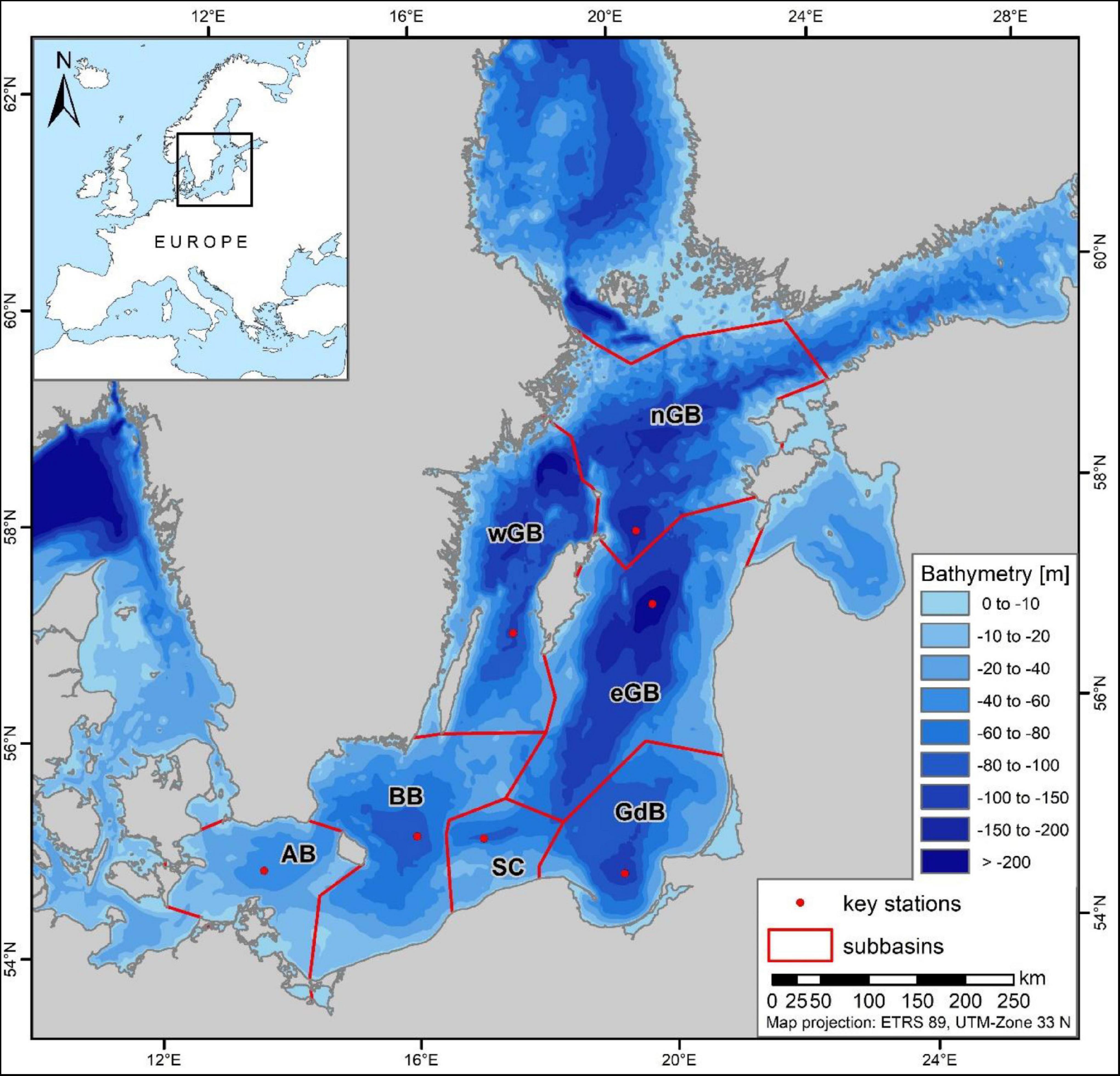
Figure 1. Bathymetry of the southern and central Baltic Sea, with basin boundaries and monitoring stations. AB, Arkona Basin; BB, Bornholm Basin; SC, Slupsk Channel; GdB, Gdansk Basin; eGB, eastern Gotland Basin; nGB, northern Gotland Basin; wGB, western Gotland Basin. The topographic information is based on the publicly available dataset “iowtopo2_rev3” for the Baltic Sea region (Seifert and Kayser, 1995; see also https://www.io-warnemuende.de/topography-of-the-baltic-sea.html, assessed on 2015-03-08).

A prerequisite for the design of measures aimed at reducing hypoxia in the Baltic Sea is an understanding of the dynamics and driving forces, both anthropogenic and physical, of hypoxia. Thus, in this study we analyzed the spatio-temporal patterns of hypoxic and euxinic areas in the Baltic Sea, including relevant trends due to anthropogenic eutrophication and the influence of two additional major drivers: stratification changes and warming. The analysis was based on novel, seasonally and basin-wide resolved observational datasets derived from mapped hypoxic and euxinic areas for 1969–2016 and comparisons thereof with other publicly available observational products (Hansson and Andersson, 2015; Almroth-Rosell et al., 2021) and two model-based, three-dimensional ocean reanalyses (Liu et al., 2017, 2019). The aim of the study is to investigate uncertainties in hypoxic and euxinic area estimates and to answer the question whether recent trends are affected by these uncertainties or whether systematic changes in oxygen conditions, e.g., caused by nutrient input reductions, can be detected. In particular, we are interested in the changes after about 1998, when the vertical stratification had rebuilt after a pronounced stagnation period 1983–1992 (Mohrholz, 2018) and when external nutrient inputs have become significantly lower compared to the 1980s (HELCOM, 2018). The latter research question is motivated by the results of ensemble model projections under the BSAP nutrient input scenario, suggesting a significant reduction in hypoxic area after the 2020s compared to the status under a reference scenario (Meier et al., 2018b, 2019c; see Figure 2). We focused on reanalysis and geostatistical mapping products because model results without data assimilation are not sufficiently accurate yet for the posed research question (Meier et al., 2019c).

FIGURE 2

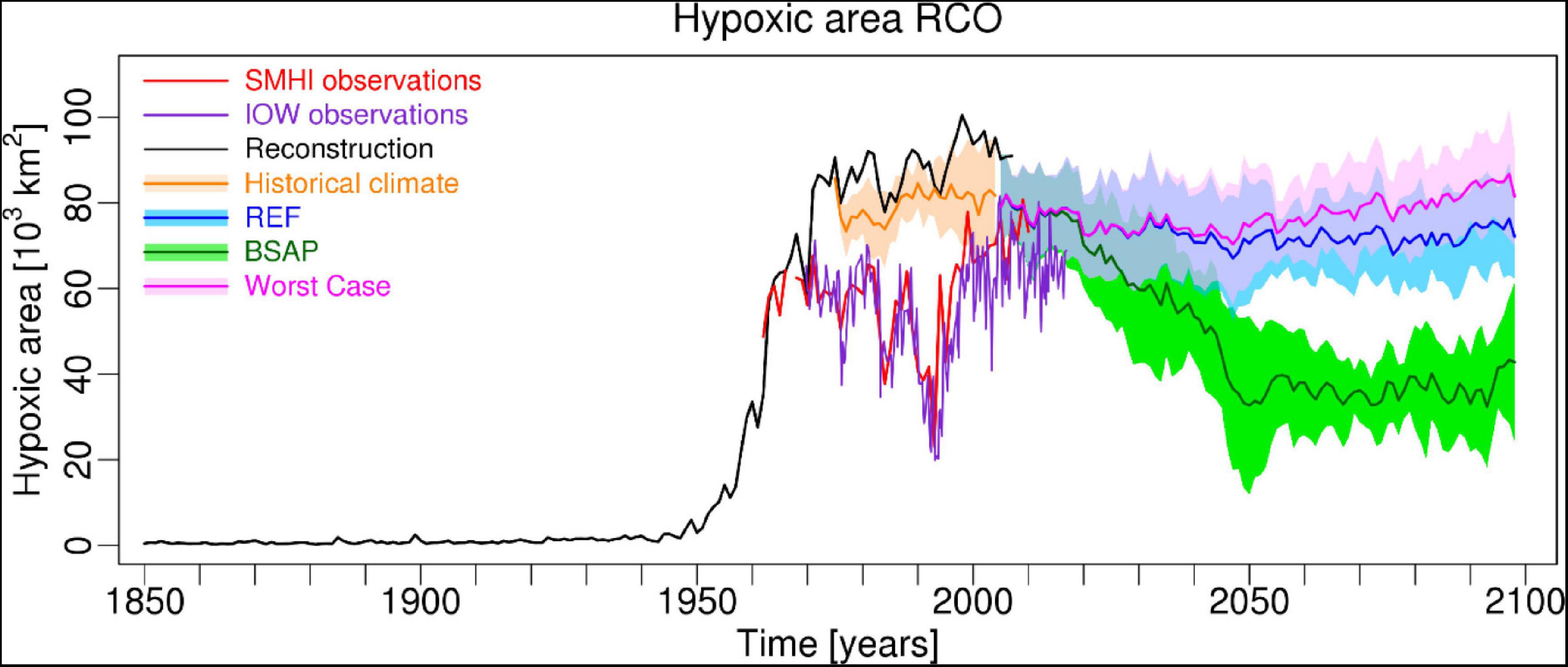
Figure 2. Simulated ensemble mean and from observations calculated hypoxic area (in 10³ km²) in the Baltic proper comprising Arkona Basin, Bornholm Basin, Gotland Basin, Gulf of Riga and Gulf of Finland. Shown are SMHI (Hansson and Andersson, 2015; red line) and IOW (this study; purple line) data. Further, a historical reconstruction starting in 1850 by Meier et al. (2019a; 2019b) is shown (black line). Finally, ensemble mean RCO model results by Saraiva et al. (2019) for the nutrient load scenarios Reference (REF, blue line), Baltic Sea Action Plan (BSAP, green line) and Worst Case (pink line) are depicted. The colored shaded areas denote the range of plus and minus one standard deviation of the ensemble member results. For details concerning scenario simulations the reader is referred to Meier et al. (2018b, 2019c). Supplementary Figure 2 by Meier et al. (2019c).

Materials and Methods

Study Area

The Baltic Sea is a shallow sea with an estuarine-like circulation that derives from its large river-borne freshwater inflows and limited connections to the North Sea (Leppäranta and Myrberg, 2009). It is almost completely enclosed by Germany, Denmark, Sweden, Finland, Russia, Estonia, Latvia, Lithuania, and Poland. The Baltic Sea proper comprises several basins: Arkona Basin, Bornholm Basin, Gdansk Basin, the eastern, northern and western Gotland sub-basins, and Slupsk Channel, which connects the Bornholm Basin to the eastern Gotland Basin (Figure 1). The large proportion of agricultural land and high population density along the Baltic Sea have led to major inputs of phosphorus and nitrogen, especially in its southern region (HELCOM, 2018).

Approach

Time series aimed at tracking the sizes of hypoxic and euxinic areas in the Baltic Sea and its basins have been collected since the 1960s. Given the dominance and size (Supplementary Figure 1) of the Bornholm Basin and the eastern, northern and western Gotland sub-basins, they are the focus of this study, together with the total area of the Baltic Sea. To investigate the correlations between physical parameters with the sizes of the hypoxic and euxinic areas in the Baltic Sea, bottom salinity and bottom temperature linked to inflow events, and halocline depth and stratification strength (Väli et al., 2013) were analyzed (Supplementary Table 1) using averaged monthly values. The seasonality of the parameters in the different basins was determined as well.

IOW Data

Since 1954, monitoring cruises aimed at investigating the environmental status and long-term variability of the Baltic Sea’s ecosystem have been regularly carried out by the Leibniz Institute for Baltic Sea Research Warnemünde (IOW) and its predecessor. The cruises cover a large area of the Baltic Sea, with data collected from up to 77 long-term stations, located from the western Baltic Sea to the central deep basins, and including measurements of physical, chemical and biological parameters (Figure 1). The annual cycle is covered by five cruises per year, conducted during fixed periods (January–February, March, April–May, July–August, and October–November). Data gaps in local regions, e.g., caused by stormy weather and other difficulties, are complemented for most of the central basins by data from the Swedish Meteorological and Hydrological Institute (SMHI) and for the Gdansk Basin since 1980 from the Polish Institute of Meteorology and Water Management (IMGW). Prior to 1980, the Gdansk Basin was well sampled by cruises of the IOW’s predecessor, the Institute for Marine Science of the German Democratic Republic (GDR). All data are quality checked, homogenized and imported into the IOW’s Oceanographic Database with Interactive Navigation (ODIN2),² allowing the use of programmed routines for further processing to mapping products.

For the interpolation/extrapolation process, an automated database request extracted from each cruise both the depths at which, according to laboratory tests, the waters became hypoxic (dissolved oxygen levels: < 2 mL L^–1) or euxinic (dissolved oxygen levels = 0 mL L^–1 and H₂S is detected) and the sea bottom values of dissolved oxygen and hydrogen sulfide concentrations. This so-called level file was geostatistically interpolated (kriging) to a one nautical mile (nm) grid, spreading the depth levels horizontally up to the margins of the basins (Feistel et al., 2016, 2022). This covered area was exported as a shape file (1-nm raster and polygons) for further processing in a geographical information system (ArcGIS). In ArcGIS, the shape files were transformed from geodetic coordinates (WGS84) to projected UTM coordinates (ETRS89), which allowed the use of metric units for spatial calculations. Area calculations were then performed for all polygon shape files and the total areas were divided by the territorial margins into areas for each of the seven basins (Arkona Basin, Bornholm Basin, Slupsk Channel, Gdansk Basin, eastern Gotland Basin, northern Gotland Basin and western Gotland Basin; see Figure 1). A MATLAB script extracted these values from each attribute table of the shape files and listed them in a text file, thus building a database for further statistical analysis (Naumann et al., 2021).

Different kriging approaches were tested and compared to a professional interpolation software using variogram analysis with a limited search radius (SURFER—Golden Software). We found that complex kriging functions did not improve the results because the spreading of hypoxia is controlled by topographic details such as sill depths and basin margins. For the mapping, more important than the usage of advanced interpolation methods is the data coverage per oceanographic unit because the data are sparse (see section “Discussion”). Hence, we decided to apply a simple interpolation approach without including trend variables and complex variogram analyses.

Dissolved oxygen measurements with sufficient coverage according to our criteria for the calculation of hypoxic area are available for all basins from October 1969 onwards, thus allowing an area-wide analysis of hypoxia in the Baltic Sea (Supplementary Figures 2, 3). However, H₂S concentrations have not been consistently measured since 1978. In this study, the threshold for adequate spatial data coverage was a minimum of three measured stations at each of the seven basins. Accordingly, 195 datasets for hypoxic areas and 181 datasets for euxinic areas were obtained and included in the statistical analysis of hypoxic and euxinic areas. Example maps depicting minimum (∼19,900 km² in February 1993) and maximum (∼81,600 km² in November 2004) hypoxic areas are shown in Supplementary Figures 4, 5.

For the correlation analysis, temperature, salinity and oxygen concentration data were extracted from ODIN2 (for mean profiles see Supplementary Figures 6–8). Data availability differed depending on the basin, depth, season and parameter (Supplementary Figures 9–11). One station within each basin was chosen to assess the physico-chemical state of that basin (Supplementary Table 2).

Other Datasets

Uncertainties related to data quality were estimated by comparing the hypoxic and euxinic areas defined by the IOW data with those described in a mapping product of the SMHI (Hansson and Andersson, 2015; Hansson and Viktorsson, 2020), in the observational dataset ALM by Almroth-Rosell et al. (2021) and in two model-based three-dimensional ocean reanalyses, i.e., the Rossby Centre Ocean model (RCO) reanalysis by Liu et al. (2017) and the Copernicus reanalysis (Reana) for the Baltic Sea by Axell et al. (2019) and Liu et al. (2019, see also Kõuts et al., 2021).

The SMHI maps are based on autumn monitoring data for the period 1960–2020, albeit with missing values for 1961 and 1967 (Hansson and Andersson, 2015). The maps cover the Baltic proper (comprising the Arkona Basin, the Bornholm Basin and the Gotland Basin), the Gulf of Finland and the Gulf of Riga and are regularly updated by the SMHI.

Almroth-Rosell et al. (2021) extracted observed oxygen data for the Bornholm Basin and eastern, northern and western Gotland Basin of all profiles during autumn (August–October) for the period 1960–2019 from the public database of the International Council for the Exploration of the Sea (ICES) Dataset on Ocean Hydrography.³ From the available profiles the depths of hypoxia and anoxia were calculated, gridded with linear interpolation (Delaunay triangulation) between sampling stations and extrapolated sideways toward the same topographic data as used within our study (Seifert and Kayser, 1995). In contrast to our study, the maps are constructed from monitoring profiles measured during 3 months while the maps in our study are based on data from one monitoring cruise and complementing data. Note that the basin boundaries differ between IOW (Figure 1) and ALM (Almroth-Rosell et al., 2021; their Figure 1) datasets and that in ALM the Arkona Basin is not included. For further details, the reader is referred to Almroth-Rosell et al. (2021).

The RCO reanalysis was performed for the period 1970–1999 using the Swedish Coastal and Ocean Biogeochemical model (SCOBI) coupled to the Rossby Centre Ocean model (RCO) for the entire Baltic Sea (Meier et al., 2003; Eilola et al., 2009; Almroth-Rosell et al., 2011), with monitoring data from the Swedish Ocean Archive (SHARK)⁴ and the Ensemble Optimal Interpolation (EnOI) method (Liu et al., 2017). In the RCO-SCOBI setup, the horizontal resolution is two nautical miles (3.7 km) and there are 83 vertical levels, with layer thicknesses of 3 m. RCO-SCOBI is forced by atmospheric forcing data calculated from regionalized ERA–40 reanalysis data (Samuelsson et al., 2011).

An independent evaluation of the RCO data and a comparison of its results with those of several different ocean circulation models were published by Eilola et al. (2011) and Placke et al. (2018). Placke et al. (2018) compared three ocean circulation models for the Baltic Sea for the period 1970–1999 and found that in all models, including RCO with and without data assimilation, seasonal cycle, variability, and vertical profiles of temperature and salinity are simulated in satisfactory agreement with observations although the models’ mean circulation differs. The latter was explained by differences in the wind forcing. Eilola et al. (2011) compared three coupled physical–biogeochemical models for the Baltic Sea with observations. Overall RCO-SCOBI, applied without data assimilation, simulated oxygen dynamics well but overestimated hypoxic area during the stagnation period 1983–1992 (Eilola et al., 2011, their Figure 10; see also Meier et al., 2019a, their Figure 11; Meier et al., 2018a, their Figure 3; and Figure 2 of this study). However, with data assimilation oxygen profiles and hypoxic area were well simulated compared to observations (Liu et al., 2017; see Figure 3 of this study).

FIGURE 3

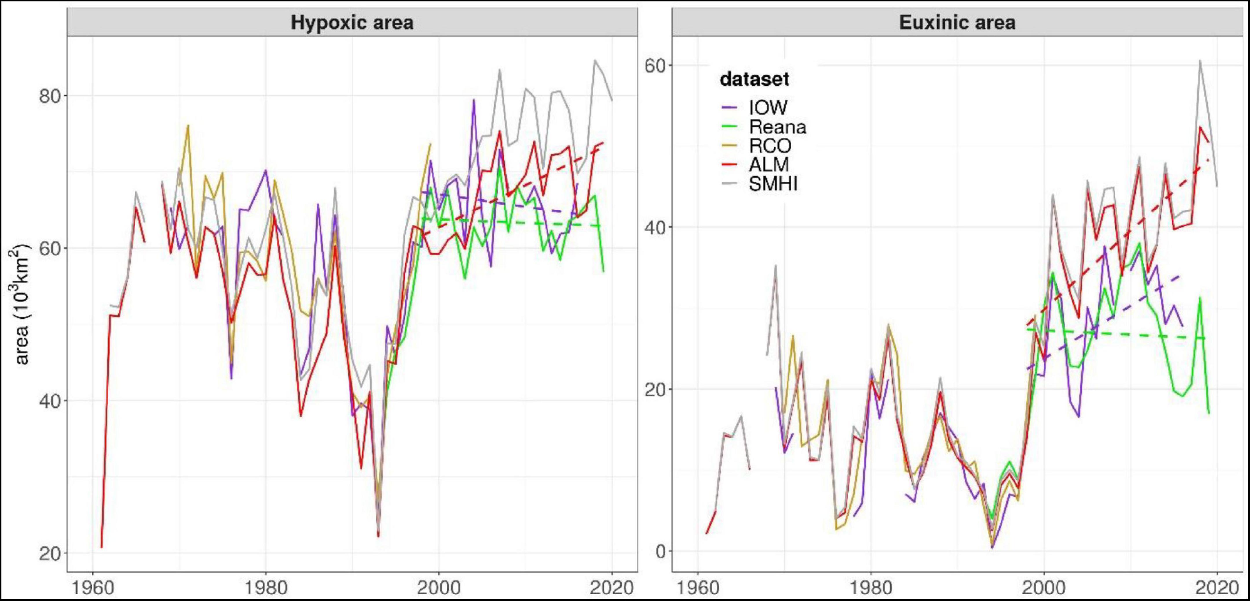
Figure 3. July–October mean hypoxic and euxinic (H₂S) areas (in 10³ km²) in the Baltic Sea as determined from the Copernicus reanalysis data (Reana), IOW data, RCO reanalysis data (RCO), ALM and SMHI data. Note that in this figure the IOW, RCO, ALM and Reana datasets do not include the Gulf of Finland and Gulf of Riga whereas the SMHI dataset does. In addition, for the datasets IOW, ALM and Reana trends since 1998 are shown and discussed in the main text (section “Results”).

The Copernicus ocean reanalysis (Reana) covers the period 1993–2019 and was obtained by employing SCOBI coupled to the NEMO 3.6 model (Nucleus for European Modelling of the Ocean version 3.6) for the North Sea–Baltic Sea (Hordoir et al., 2015; Pemberton et al., 2017). This reanalysis assimilated sea surface temperature observations at the SMHI (from the SMHI’s Swedish Ice Service) as well as in situ measurements for temperature and salinity from the ICES database (Liu et al., 2019) and nitrate, phosphate, ammonium and oxygen observations from SHARK (Axell et al., 2019). For the assimilation, the Localized Singular Evolutive Interpolated Kalman (LSEIK) filter (Nerger et al., 2005) was used. The NEMO-SCOBI setup applied a horizontal resolution of two nautical miles (3.7 km) and 56 vertical levels, with layer thicknesses between 3 m close to the surface and 22 m at the bottom of the deepest part of the model domain, located in the Norwegian trench. During the course of this reanalysis, the applied atmospheric forcing was changed from the Euro4M atmosphere reanalysis (22 km), used until 2011, to the UERRA reanalysis (11 km), beginning in 2012. For details the reader is referred to Axell et al. (2019) and Liu et al. (2019).

For an overview about the compared datasets the reader is referred to Table 1.

TABLE 1

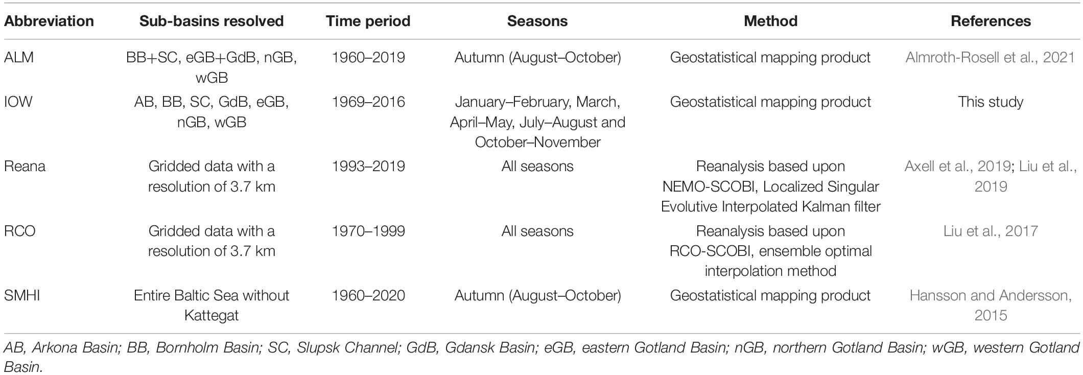
Table 1. Overview about the utilized datasets.

Analysis

A basin based analysis of open-water hypoxia and euxinia was carried out. Pressure (in dbar units) was used as an indicator of depth. Other parameters and units were: hypoxic area (km²), euxinic area (km²), halocline depth (dbar), stratification strength (g kg^–1), bottom salinity (g kg^–1) and bottom temperature (°C). Halocline depth was defined as the maximum vertical gradient criterion, as in the study of Väli et al. (2013). To exclude the potential inclusion of an existing upper seasonal halocline, a range of permanent halocline depths was considered, separately for each basin (HC in Supplementary Table 3). Stratification strength was defined according to Väli et al. (2013) as the difference between the salinity of the top (0–60 m depth) and bottom (> 60 m depth) layers (ST in Supplementary Table 3). Bottom salinity and temperature were determined based on the deepest measured value below a threshold depth, below which the parameter values remained constant (BS, BT in Supplementary Table 3).

For the IOW, RCO and Reana datasets, the seasonal anomalies were derived relative to the annual mean over the whole period. Then the means for each season and the 95% confidence intervals were calculated.

Following for instance Kniebusch et al. (2019), the residual bottom temperature, BTr, is additionally used, defined as the difference between the bottom temperature, BT, and the linear regression of the bottom salinity, BS, as the explanatory variable, on the bottom temperature, BT, as the dependent variable, i.e., BTr = BT—(a BS + b) with

$a=\frac{{\sum }_{i=1}^n(B{S}_i-\overline{BS})(B{T}_i-\overline{BT})}{{\sum }_{i=1}^n{(B{S}_i-\overline{BS})}^2}$

$b=\overline{BT}-a\overline{BS}$

Removing the co-variation between salinity and temperature from the original temperature record allows to approximately disentangle the bottom temperature variations due to MBIs and due to long-term changes such as climate change.

Results

Dynamics of Hypoxic and Euxinic Areas

Figure 3 shows the temporal evolution of hypoxic and euxinic areas according to five different datasets. To allow a comparison with the IOW and ALM data, hypoxic and euxinic areas of the RCO and Reana datasets shown in Figure 3 do not include the hypoxic and euxinic areas in the Gulf of Finland and Gulf of Riga because the IOW and ALM datasets do not consider those basins. In Supplementary Figure 12, uncertainty ranges based upon four datasets, i.e., IOW, ALM, RCO and Reana and trends since 1998 are shown.

The hypoxic area of the Baltic Sea (Figure 3, left) in 1970 was large, ∼60,000 km² or ∼60% of the entire bottom area below the halocline in the Baltic proper according to the IOW dataset (Supplementary Figure 13), but by 1993 it covered only ∼20,000 km². Thereafter, there was a strong increase until around the year 2000, with the size of the area (∼65,000 km²) nearly the same as in 1970. Then, until 2016, the size of the hypoxic area remained essentially unchanged. The four different datasets starting 1970 or earlier show a similar development of the Baltic Sea’s hypoxic area until ∼2000, after which the data diverge.

The euxinic/anoxic area of the Baltic Sea (Figure 3, right) strongly fluctuated, nearly disappearing by 1994 but strongly expanding until 2000, a finding common to all four datasets. Afterward, while the ranges in the IOW and Reana euxinic datasets are the same (20–40,000 km²), according to the SMHI and ALM data the anoxic area grew to > 40,000 km² after 2000.

A basin based analysis of the hypoxic area in autumn (Figure 4, upper row) shows major differences. The pattern of hypoxia was similar in the three Gotland sub-basins and their contributions to the total hypoxic area in the Baltic Sea were the largest, due to their geomorphology and size (15,000–25,000 km² in their maximum extent). In those basins, hypoxia steadily decreased, albeit with some fluctuations, until around 1993 (e.g., in the eastern Gotland Basin from ∼21,000 km² in 1981 to ∼8,000 km² in 1993 according to the IOW dataset) but then rose again abruptly (Figure 4, upper row). In the other, smaller basins hypoxia-free conditions were eventually reached, unlike in the Gotland sub-basins (not shown). The hypoxic areas in the Gotland sub-basins plateaued by 2000, reaching a size similar to or only slightly larger than the size of the hypoxic area in the 1970s, before the major drop. For the Bornholm Basin, the pattern in the RCO and Reana data is similar to that of the IOW data, with differences only in the strength of the deflections. In the Gotland sub-basins, the RCO and Reana data closely follow the IOW data. Hypoxic areas from the ALM dataset are larger in the Bornholm Basin and eastern Gotland Basin but smaller in the northern Gotland Basin compared to the IOW data because of the different location of basin boundaries. The SMHI data do not resolve the individual basins and therefore are not included in Figure 4.

FIGURE 4

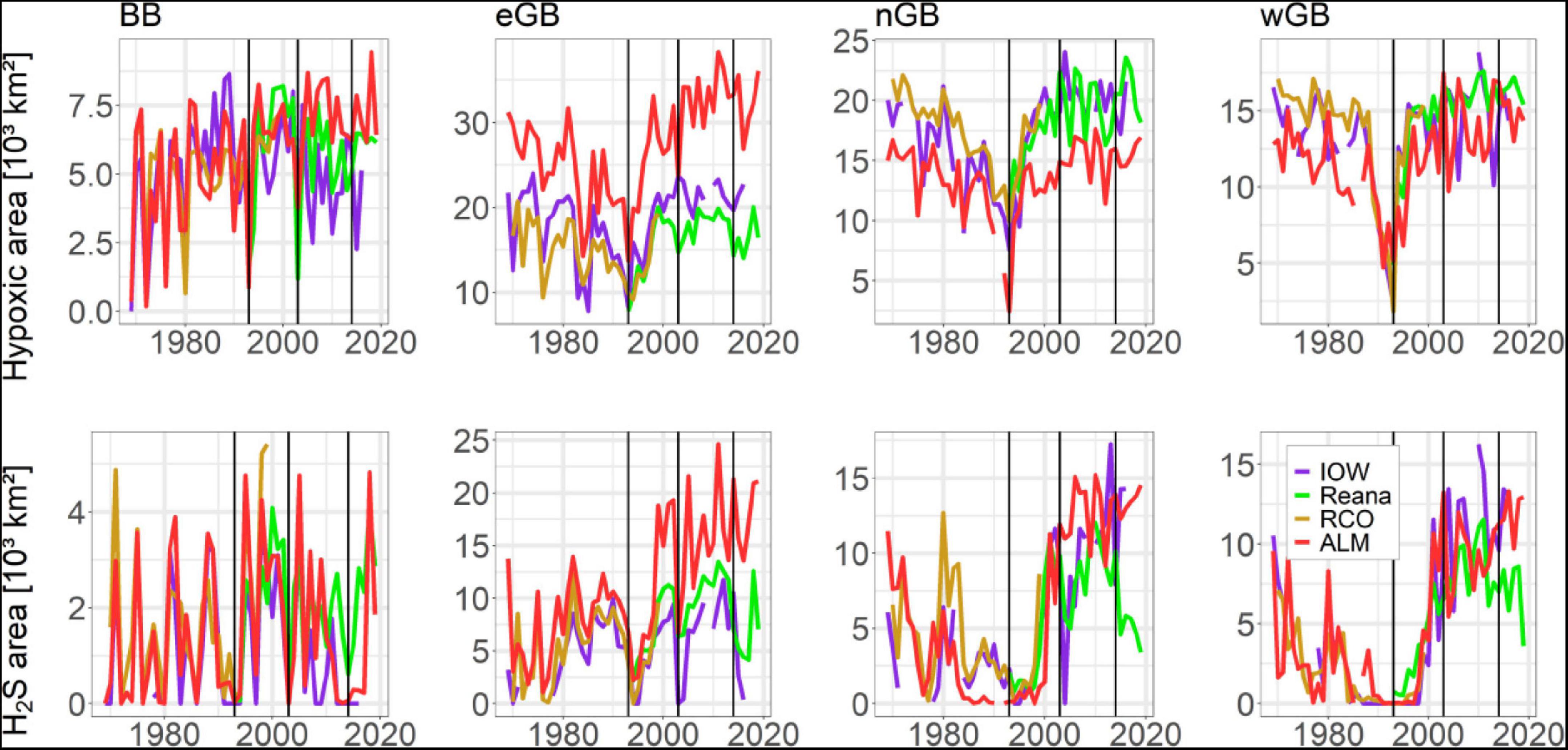
Figure 4. July–October mean hypoxic and euxinic (H₂S) areas (in 10³ km²) in selected basins as determined from the Copernicus reanalysis data (Reana), IOW data, ALM data and RCO reanalysis data. BB, Bornholm Basin; eGB, eastern Gotland Basin; nGB, northern Gotland Basin; wGB, western Gotland Basin. Vertical black lines mark the Major Baltic Inflows in 1993, 2003, and 2014.

While the size of the euxinic area (Figure 4, lower row) in the Bornholm Basin during the study period widely fluctuated, between 0 and 4,000 km², in the Gotland sub-basins it increased substantially, reaching unprecedented extents of 10–15,000 km², i.e., ∼10–15% of the entire bottom area below the halocline in the Baltic proper according to the IOW data (Supplementary Figure 13). Minimum values occurred mostly before 2004 (e.g., no euxinia in 1994/1995 in the eastern and western Gotland Basin and in 2004 in the eastern Gotland Basin). For the Gotland sub-basins, the RCO data agree very well with the IOW data. However, the Reana data for the eastern Gotland Basin indicate smaller fluctuations and an euxinic area slightly larger than that based on the IOW data, while for the northern and western Gotland sub-basins most values are below those of the IOW data. In the Gotland sub-basins, the anoxic areas from the ALM dataset are usually larger compared to the euxinic areas from the IOW data.

According to the IOW data, the hypoxic area over the entire Baltic Sea was never as large as the size that would be reached at halocline depth (Supplementary Figure 13). The hypoxic areas of the southwestern basins (Arkona and Bornholm) as well as the Slupsk Channel were less than half the size of the bottom area below the halocline. By contrast, the hypoxic area in the large, deep Gotland sub-basins approached that at halocline depth. This difference clearly distinguished the southwestern from the central basins of the Baltic Sea.

In summary, based upon the IOW data the annual mean hypoxic and euxinic areas for the period 1969–2016 amount to 55,700 and 14,600 km², respectively, or ∼55 and 14% of the entire bottom area below the halocline in the Baltic proper (Supplementary Table 4). The corresponding standard deviations are 13,100 and 9,900 km². Hence, hypoxia and euxinia in the Baltic Sea show a large interannual to decadal variability.

The differences between IOW and ALM data are summarized by Table 2. These datasets cover roughly the same period, while the periods of the reanalyses (RCO and Reana) are considerably shorter. Hypoxic areas of the Bornholm Basin and Gotland Basin are similar. Differences are well explained by different basin boundaries, and similar results are obtained by summarizing hypoxic areas of both Slupsk Channel and Bornholm Basin and Gdansk Basin and eastern Gotland Basin of the IOW dataset. However, the larger discrepancies in euxinic areas can likely not be explained by differing basin boundary definitions.

TABLE 2

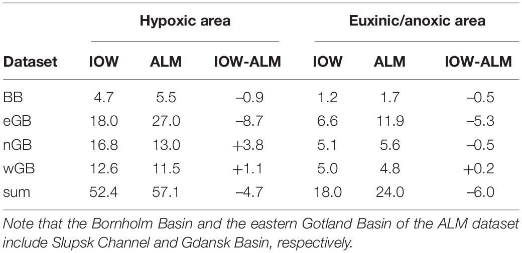
Table 2. Mean hypoxic and euxinic/anoxic areas (in 10³ km²) of IOW and ALM datasets for common years with data in Bornholm Basin (BB), eastern (eGB), northern (nGB), and western Gotland (wGB) sub-basins and the sum.

Seasonal Cycle

Both hypoxic and euxinic areas are subject to a pronounced seasonal cycle (Figure 5). According to the IOW dataset, the hypoxic area was smallest in spring in the entire Baltic Sea and in the Bornholm Basin; in spring, summer and fall in the eastern Gotland Basin, in winter in the northern Gotland Basin and in winter and spring in the western Gotland Basin. The hypoxic area reached a maximum in autumn in the Baltic Sea and in the Bornholm Basin and western Gotland Basin, in winter in the eastern Gotland Basin and in summer in the northern Gotland Basin. The euxinic area in the Baltic Sea in general and in the northern and western Gotland sub-basins specifically had a strong summer maximum, whereas in the Bornholm Basin the maximum size was reached in autumn and in the eastern Gotland Basin in winter. The reanalysis datasets, Reana and RCO, show a similar seasonality as the IOW data but also shifts in the maxima and minima to adjacent seasons.

FIGURE 5

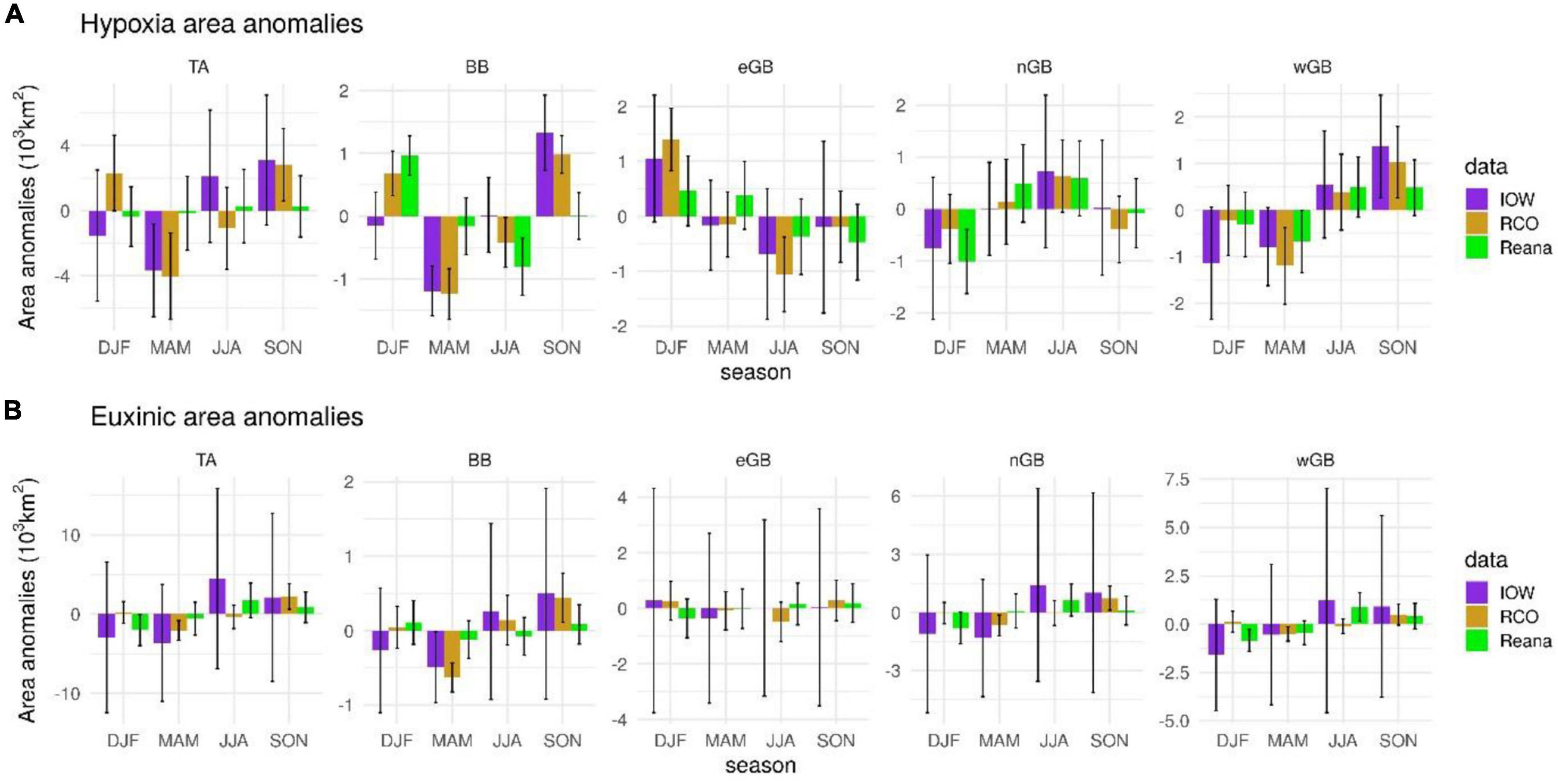
Figure 5. Seasonal anomalies in (A) hypoxic (HYP) and (B) euxinic (H2S) areas and 95% confidence levels (in 10³ km²) in the total area of the Baltic Sea (TA), the Bornholm Basin (BB) and in the eastern, northern and western Gotland sub-basins (eGB, nGB, wGB) according to the IOW, RCO and Copernicus reanalysis (Reana) datasets.

As the largest seasonal extents of the hypoxic areas occurred mainly in autumn (Figure 5), this season was the focus of the analysis summarized in Figure 4. In this figure, IOW data are based upon the average hypoxic or euxinic area from the cruises in July/August and October/November. According to the IOW dataset, the size of the hypoxic areas in the Gotland sub-basins remained largely unchanged after 1998 whereas in all three the size of the euxinic areas depended on the strengths of the MBIs (Figure 4). These results suggest that, by the end of the study period, the hypoxic areas in the Gotland sub-basins had reached their maximum possible size (Supplementary Figure 13) and further increases are unlikely because both hypoxic and euxinic areas are limited by the depth of the halocline.

Trends Since 1998

According to our investigations, we could not find statistically significant changes at the 95% confidence level in hypoxic and euxinic areas throughout the Baltic Sea since 1998, which have the same sign in all three datasets, i.e., IOW, ALM and Reana, so-called robust trends (Figure 3 and Supplementary Figure 12). For the hypoxic areas, only the ALM dataset shows a statistically significant increase, while the other two datasets, IOW and Reana (Figure 3), and the ensemble mean (Supplementary Figure 12) do not systematically change. For the euxinic area, only the trends in the ensemble mean and the maximum of the anoxic/euxinic area are statistically significant at the 95% confidence level (Supplementary Figure 12), as the anoxic area increases in ALM and the euxinic area in IOW (Figure 3). However, it should be noted that the IOW dataset ends in 2016 and the three consecutive years 2016–2019 may change the slope as in Reana, which shows no statistically significant trend in euxinic area. Prior to 2016, the sizes of hypoxic and euxinic areas of IOW and Reana datasets agree well. Why the two datasets, ALM and Reana, significantly differ in their long-term trends since 1998 is unknown. For further details about the trends in Reana the reader is referred to Kõuts et al. (2021).

Physical Drivers of Hypoxic and Euxinic Areas

Figure 6 shows the results of the correlation analysis between hypoxic and euxinic areas of the IOW database and halocline depth, stratification strength, bottom salinity, bottom temperature and residual bottom temperature calculated from observations at central monitoring stations (Figure 1) extracted from ODIN2. A negative correlation of halocline depth and stratification strength in all basins implies that a deep halocline is related to weak stratification, and a shallower halocline to stronger stratification (Figure 6). In the Gotland sub-basins, the correlation between bottom salinity and bottom temperature, with a high bottom salinity corresponding to a high bottom temperature, reflects the warmer temperature of saltwater inflows than of the surrounding water (Figure 6). These results suggest that bottom salinity and bottom temperature are not necessarily independent drivers of hypoxia and euxinia. Hence, Figure 6 also shows the correlations between the residual bottom temperature, defined as the difference between the bottom temperature and the linear regression of the bottom salinity, as the explanatory variable, on the bottom temperature, as the dependent variable (section “Materials and Methods”).

FIGURE 6

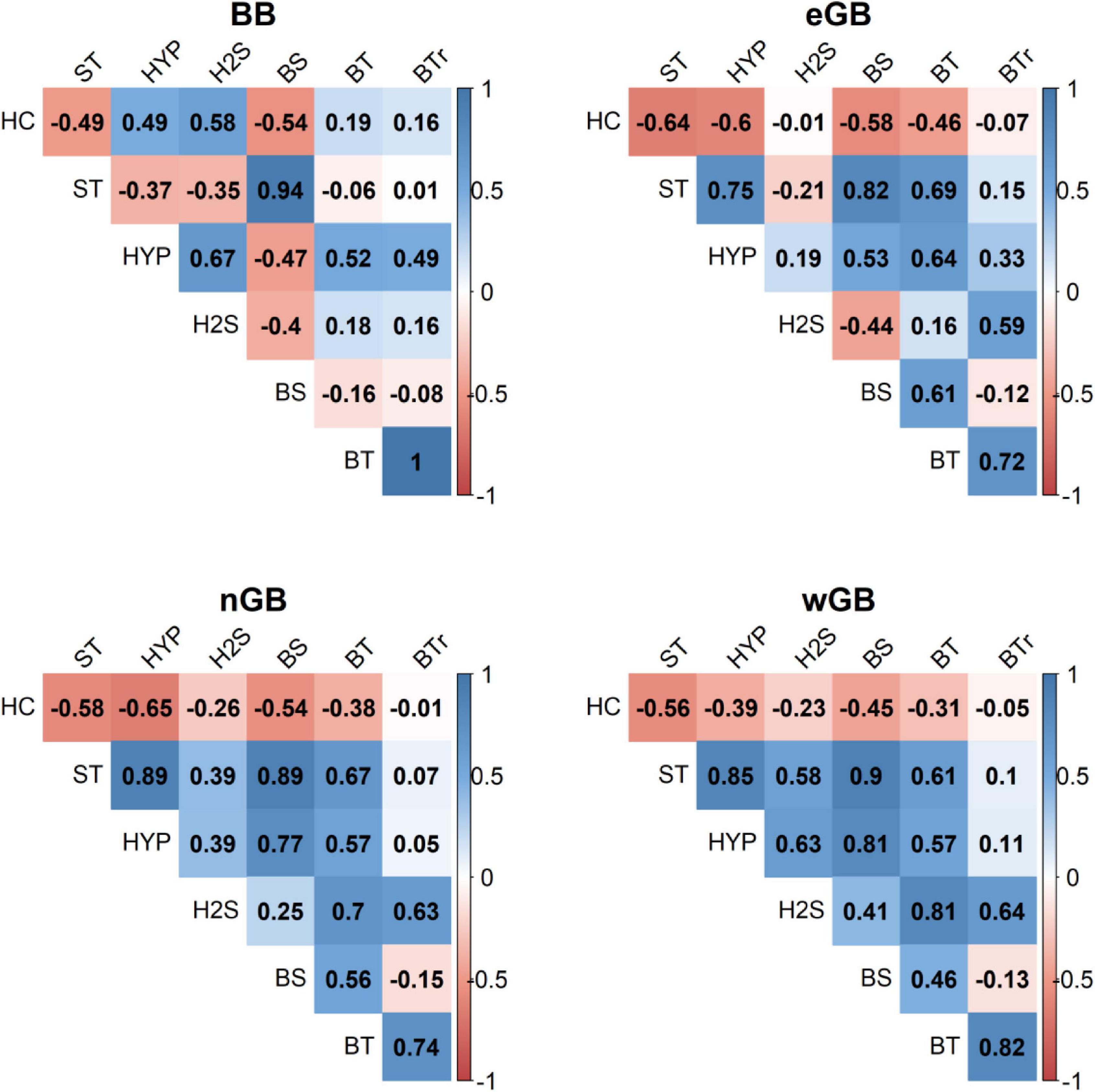
Figure 6. Correlations between hypoxic (HYP) and euxinic (H2S) areas, halocline depth (HC), stratification strength (ST), bottom salinity (BS), bottom temperature (BT) and residual bottom temperature (BTr) in the Bornholm Basin (BB), eastern Gotland Basin (eGB), northern Gotland Basin (nGB) and western Gotland Basin (wGB). The residual bottom temperature (BTr) is defined as the difference between the bottom temperature (BT) and the linear regression of the bottom salinity (BS), the explanatory variable, on the bottom temperature (BT), the dependent variable.

In most cases the physical variables correlate strongly with the size of the hypoxic area (Figure 6). In the Bornholm Basin, the hypoxic area is larger when the bottom salinity is lower and the residual bottom temperature higher, and when the halocline is deeper and stratification weaker. The hypoxic area maximum often coincides with the maximum size of the euxinic area, and both are strongly linked to a deeper halocline.

In the three Gotland sub-basins, the hypoxic area strongly correlates with stratification and inflow parameters (halocline depth, stratification strength, and bottom salinity). A shallower halocline, a stronger stratification as well as increased bottom salinity are related to a larger hypoxic area. In all three Gotland sub-basins, a large euxinic area is related to a high residual bottom temperature. In the western Gotland Basin the size of the euxinic area also correlates positively with stratification strength.

Discussion

Data Availability and Data Accuracy

Temporal Undersampling

Profiles of temperature and salinity used for the correlation analysis and the IOW data of hypoxic and euxinic areas for the study period are irregularly distributed over time. Hypoxia maps have been available since October 1969 for all basins. The availability of monitoring data strongly depends on the decade, the basin, the depth profile and the season (Supplementary Figures 2, 3, 9–11). H₂S has only been measured continuously since 1978. The new IOW dataset is, however, representative and well supported by the time series data of the other datasets prior to 1993, but also after that, especially by Reana.

Spatial Undersampling

An estimation of the error bars was performed by reducing the number of the monitoring stations used to calculate the maps by about two-thirds for the period 2000–2016. This time period comprises 77 maps out of 195 for the entire period 1969–2016. On average 64 stations (maximum 77), spanning from the western to the central Baltic Sea, form the original dataset for the mapping (Supplementary Figure 14; red and white dots). From these stations, on average ∼23 were selected (minimum 12, maximum 27 depending on the availability from the corresponding cruise) that were used for processing of the maps (Supplementary Figure 14; red dots). In general, hypoxic and euxinic areas between the two datasets match well (Supplementary Figure 15). However, hypoxic and euxinic areas calculated with the reduced dataset are larger compared to the figures calculated with the entire dataset by on average +2,230 km² (+3.8%) and +423 km² (+3.7%), respectively. Only a few outliers occurred, with a maximum of +37% for hypoxic area and +48% for euxinic area. Hence, we conclude that the IOW interpolation method can reasonably cope with patchy datasets and lead to appropriate results with acceptable error bars. Nonetheless, calculations of the halocline depth for the correlation analysis should be viewed critically, as the halocline depth can extend over a range of 10–20 m.

Differences Between Datasets

The Reana dataset does not begin until 1993 but, since then, its temporal evolution agree well with that of the IOW data (Figure 3). However, despite data assimilation, which results in only small biases at central stations (Supplementary Figures 6–8), the accuracy of this model simulation is not perfect. Differences in hypoxic and euxinic areas between Reana and IOW/RCO data might among others be explained by different topographical data. In the NEMO-SCOBI model the topography was smoothed, resulting in a shallower Gotland Deep region with maximum differences in depth of ∼50 m compared to the topographical data by Seifert and Kayser (1995), see different profile depths in Supplementary Figures 6–8. Furthermore, the spatial resolution of assimilated biogeochemical observations from SHARK is coarser than that of the IOW dataset. Hence, trends in bottom oxygen concentration at locations without data assimilation such as the southwestern Baltic Sea might not be reliable. For instance, we found in Reana trends since 1993 with opposite sign compared to in situ measurements in Mecklenburg Bight (not shown). Nevertheless, the overall agreement in hypoxic and euxinic area between Reana and IOW datasets is regarded as good.

The differences between SMHI and ALM datasets of hypoxic area are likely explained by the increased hypoxia in the Gulf of Finland and Gulf of Riga after 2000 (Stoicescu et al., 2019, 2021).

The differences between IOW and ALM datasets of hypoxic and euxinic/anoxic areas are estimates of the errors due to different numbers and locations of profiles, different length of the measurement period (2 weeks vs. 3 months), different interpolation methods and different boundaries of the basins. Most of the differences at basin-scale might be explained by different basin boundaries (Table 2). However, it is unknown why euxinic areas of the IOW dataset are systematically smaller than anoxic areas of the ALM dataset (during 2014–2016 maximum differences amount to ∼10,000 km²).

Seasonal Cycle

Seasonal maxima of hypoxia are caused by the accelerated oxygen depletion that follows spring and summer algal blooms, during which organic material decomposes. Inflow activities and storms in the Baltic Sea occur mainly in winter and result in a mixing of its water layers, a weakening of stratification and better oxygen distribution. The southwestern basins are more exposed to inflows from the North Sea, which explains the large seasonal differences in the size of their hypoxic areas detected in our study (Figure 5). As the inflows do not arrive at the same time in every basin, mixing and ventilation typically occur earlier in the Arkona Basin than in Slupsk Channel. In addition, algal blooms show a systematic seasonal shift from south to north depending on light, nutrient and temperature conditions (Hjerne et al., 2019). According to our results, during the study period, the hypoxia maximum in the Arkona Basin was in summer, but it occurred in autumn in the Bornholm Basin and in winter in Slupsk Channel. Proportionally less seasonal variations were seen in the more distant and deeper basins, which would account for their permanent large-scale hypoxia and anoxia. The northern Gotland Basin is exposed to deep water inflows from the Gulf of Finland in the east (Giesse et al., 2020). Due to the long water residence times of the northern and eastern basins, their seasonality is minimal and their reactions to the influences of winter inflows clearly delayed. Thus, an MBI from a winter storm, for example, may not reach the central Baltic Sea until spring.

Physical Drivers of Hypoxic and Euxinic Areas

The chosen proxy parameters of inflows and stratification well explained a large proportion of the interannual variability of hypoxia, especially in basins with a long water residence time. In the Gotland Basin, interannual variations in hypoxia were well explained by stratification (explained variance of 0.75² = 56% and 0.89² = 79% in the eastern and northern Gotland sub-basins, respectively, see Figure 6). Changes in vertical oxygen transport, here estimated by changes in stratification and the position of the halocline, strongly influenced hypoxia in the Gotland sub-basins, as also reported by Conley et al. (2002). However, the extent of the euxinic area was only slightly (northern and western Gotland sub-basins) or not at all (eastern Gotland Basin) explained by stratification. Instead, in all three Gotland sub-basins, the size of the euxinic area was linked to the residual bottom temperature (explained variance: 0.6² = 36%, see Figure 6). Due to a greater decomposition of organic matter and due to a lower oxygen solubility in warmer bottom water (e.g., Stigebrandt and Andersson, 2020), the euxinic area increased with the bottom temperature, even on time scales that were larger than those of the direct influence of individual saltwater inflows. The correlations between the hypoxic area and the physical drivers of basins closer to the North Sea connection (Arkona and Bornholm basins, Slupsk Channel) were relatively weak, although for the Bornholm Basin the stronger correlations with physical factors could be attributed to its longer water residence time compared to the Arkona Basin (e.g., Lass et al., 2005; Meier, 2007).

Shallow basins heat up and mix faster than do larger and deeper ones (Reissmann et al., 2009), as demonstrated by the Arkona Basin, where bottom temperatures are significantly higher in summer and autumn than in winter and spring. As the basins close to the North Sea are also exposed to many small- and medium-size inflows that do not reach the large basins (Lass and Mohrholz, 2003), bottom salinity and temperature did not correlate (Figure 6). In late summer and autumn, these are mainly warm inflows that can lead to large fluctuations in the bottom temperature (Mohrholz et al., 2006).

The behavior of hypoxia can be understood by examining ventilation processes and their dynamics in the basins, as both vary widely within the Baltic Sea. The southwestern basins are ventilated by inflows, consistent with the well-ventilated and thus oxygen-rich surface waters at the North Sea–Baltic Sea transition. In the short term, large inflows also lead to ventilation of the deep Gotland sub-basins, such that the euxinic area is spontaneously reduced in size or, depending on the extent of the MBI, disappears completely. For example, euxinic areas in the deep water of the Gdansk Basin and the eastern and western Gotland sub-basins did not occur after the 1993 and 2003 inflows (Figure 4), thus indicating that the oxygen-depleted zones were briefly ventilated. However, large inflows are associated with subsequent increases in salinity and stratification in these basins such that this secondary effect increases the size of oxygen-depleted area in the long term (Conley et al., 2002). The elevated halocline and greater stratification prevent water exchange between layers, resulting in the further isolation of the deep layer and the counteracting of both water exchange and oxygen input.

Lower correlation values (Supplementary Figure 16) indicate that the ALM dataset is slightly less suitable than the IOW dataset for investigating the response of hypoxic and euxinic areas to inflows using observations at central monitoring stations (Figure 1) due to the differently chosen basin boundaries.

Long-Term Trends

Due to the large effect of the stagnation period 1983–1992 and the MBI in 1993 on hypoxia, systematic long-term trends related to eutrophication for the periods since 1960, for which there are observational datasets, could not be investigated (Supplementary Figure 12). However, several model studies suggested that at multidecadal time scale eutrophication is the main driver of hypoxia (Gustafsson et al., 2012; Carstensen et al., 2014a; Meier et al., 2019a,b). Hence, the background forcing on bottom water oxygen concentrations is very likely related to eutrophication.

According to our result, trends in hypoxic and euxinic areas since 1998 are not yet robust, probably because the records are too short compared to the large interannual variability and compared to the long response time scale of biogeochemical cycles in the water and in the sediment of the Baltic Sea. Furthermore, uncertainties of the datasets are considerable.

Relevance for Other Coastal Seas

The countries bordering the Baltic Sea maintain an extensive environmental monitoring program since the end of the nineteenth century in order to detect changing climate of the Baltic Sea and changes in the environmental status. As outlined in the introduction, human-made hypoxia due to nutrient inputs from land is of particular concern (HELCOM, 2018). Hence, observational data products of high accuracy such as reanalyses and mapping products are needed in order to provide reliable information at the basin-scale. We compared various, publicly available datasets of hypoxic and euxinic/anoxic areas of the Baltic Sea and introduced a new one. We estimated the uncertainty due to the undersampling of large temporal and spatial variations. These findings, which are important for the design of monitoring programs and data products, might be of interest for other coastal systems prone to hypoxia such as the northern Gulf of Mexico, Chesapeake Bay, the Gulf of St. Lawrence, the northwestern Black Sea, the northern Adriatic Sea and the East China Sea (e.g., Fennel and Testa, 2019) or large lakes (e.g., Xu et al., 2021). The hypoxic area of only the six listed coastal seas together with the Baltic Sea amount to about 131,000 km² (the size of Greece) (Rabalais et al., 2010; Fennel and Testa, 2019), which is about 53% of the total hypoxic area in the coastal zone worldwide, emphasizing the importance to understand their hypoxia dynamics (Diaz and Rosenberg, 2008). In several of these coastal and lake systems, the relationship between drivers of hypoxia, i.e., nutrient inputs from land and physical factors such as water temperature and stratification, were earlier studied with the help of measurements and geostatistical methods, e.g., in the Gulf of Mexico (Obenour et al., 2013), in the Lake Erie (Xu et al., 2021), and in the Chesapeake Bay (Zhou et al., 2014). In contrast to many other systems, the interannual variability of hypoxia in the Baltic Sea is not controlled by external nutrient inputs because of the dominant impact of physical drivers and related internal nutrient loads from the sediments at this time scale (Conley et al., 2002). Due to the long responds time in the Baltic Sea, changes in hypoxia due to nutrient input changes will not be detectable for decades (Gustafsson et al., 2012). Hence, a comparison between various coastal seas and lakes might help to unravel the importance of various drivers of hypoxia.

Conclusion

The analysis of the IOW maps of hypoxia and euxinia clearly showed that a basin based approach is needed, as the basins differ considerably in their morphology and hydrodynamics. Savchuk (2018) also found that the Baltic Sea cannot be considered as a homogeneous entity, given the many local differences. Furthermore, our results showed that the different physical characteristics of the basins account for the varying dynamics of hypoxia. Inner basins are better ventilated over the long-term, when their waters are less-stratified, i.e., during periods with few MBIs. Basins close to the North Sea are mainly ventilated by oxygen-rich small to large inflows. The stable stratified system of the Gotland Basin is less influenced by the seasons than either the Arkona Basin or the Bornholm Basin, both of which have distinct seasonal cycles.

In the large Gotland Basin, the dynamics of hypoxia is well explained by vertical oxygen transports as estimated in this study from a vertical stratification proxy, whereas euxinia changes are mainly associated with long-term changes in oxygen depletion as estimated here from the residual bottom temperature changes that may not directly be related to saltwater inflow dynamics. The latter finding suggests that climate change has already played an important role by enhancing the decomposition of organic matter in the water column and in the sediment. Hence, climate change can be expected to play an even more important role in the future. As the expansion of hypoxia is restricted by the upper limit resulting from the halocline position and ventilation, the hypoxia maximum was reached before the long-lasting stagnation period of 1983–1992. Since then, the oxygen content within the hypoxic zone has steadily decreased such that the euxinic area has actively expanded.

Although we found an overall agreement between the various available hypoxia datasets, their uncertainties and the pronounced internal variability prevent the hoped-for detection of negative trends in hypoxic area attributed to the ongoing nutrient load reductions since the 1980s.

Data Availability Statement

Observational monitoring data are publicly available from the Oceanographic Database with Interactive Navigation at the Leibniz Institute for Baltic Sea Research Warnem nde (IOW) (https://odin2.io-warnemuende.de/IOW). Maps showing hypoxic and euxinic areas based upon the IOW data are available from https://www.io-warnemuende.de/hypoxic-and-anoxic-regions-in-the-baltic-sea-1969.html. The sizes of hypoxic and euxinic areas since 1954 as well as the corresponding statistics as analyzed in this study and shown in the figures and the source code of the program “GisAnox” are publicly available from the IOW’s doi server https://doi.io-warnemuende.de/10.12754/data-2021-0006 and http://doi.io-warnemuende.de/10.12754/prog-2022-0001, respectively.

Author Contributions

KK performed the data analysis and wrote a first draft of the manuscript. MN extracted the observations and constructed the hypoxic area maps separated in basins, calculated the areas and statistical values as basis of this study. CD extracted the reanalysis data and calculated the areas and statistical values separated in basins as the basis of this study. HEMM designed the research, supervised the work and wrote the final version of the manuscript with the help of all authors.

Funding

The research presented in this study was part of the Baltic Earth program (Earth System Science for the Baltic Sea region, see http://www.baltic.earth) and was partly funded by the Swedish Research Council for Environment, Agricultural Sciences and Spatial Planning (Formas) through the ClimeMarine project within the framework of the National Research Programme for Climate (grant no. 2017-01949).

Conflict of Interest

The authors declare that the research was conducted in the absence of any commercial or financial relationships that could be construed as a potential conflict of interest.

Publisher’s Note

All claims expressed in this article are solely those of the authors and do not necessarily represent those of their affiliated organizations, or those of the publisher, the editors and the reviewers. Any product that may be evaluated in this article, or claim that may be made by its manufacturer, is not guaranteed or endorsed by the publisher.

Acknowledgments

We thank the Leibniz Institute for Baltic Sea Research Warnemünde (IOW) for continuous long-term data acquisition spanning from the western to the Central Baltic Sea, and the Federal Maritime and Hydrographic Agency Hamburg and Rostock (BSH) for financing the measurements in the German Exclusive Economic Zone (EEZ) as part of the National Environmental Monitoring Programme. We thank Hagen Radtke, IOW, for support with R programming for the analysis and Berit Recklebe, IOW, for technical support. We thank the reviewers for their constructive comments that helped to improve the manuscript.

Supplementary Material

The Supplementary Material for this article can be found online at: https://www.frontiersin.org/articles/10.3389/fmars.2022.823476/full#supplementary-material

Footnotes

1. ^ https://helcom.fi/baltic-sea-action-plan/
2. ^ https://odin2.io-warnemuende.de/
3. ^ http://www.ices.dk/
4. ^ http://sharkweb.smhi.se

References

Almroth-Rosell, E., Eilola, K., Hordoir, R., Meier, H. E. M., and Hall, P. O. J. (2011). Transport of fresh and resuspended particulate organic material in the Baltic Sea - a model study. J. Mar. Syst. 87, 1–12. doi: 10.1016/j.jmarsys.2011.02.005

CrossRef Full Text | Google Scholar

Almroth-Rosell, E., Wåhlström, I., Hansson, M., Väli, G., Eilola, K., Andersson, P., et al. (2021). A regime shift toward a more anoxic environment in a Eutrophic Sea in Northern Europe. Front. Mar. Sci. 8:799936. doi: 10.3389/fmars.2021.799936

CrossRef Full Text | Google Scholar

Andersen, J. H., Conley, D. J., Dromph, K., Fleming-Lehtinen, V., Gustafsson, B. G., Josefson, A. B., et al. (2017). Long-term temporal and spatial trends in eutrophication status of the Baltic Sea. Biol. Rev. 92, 135–149. doi: 10.1111/brv.12221

PubMed Abstract | CrossRef Full Text | Google Scholar

Axell, L., Liu, Y., Jandt, S., Lorkowski, I., Lindenthal, A., Verjovkina, S., et al. (2019). Baltic Sea Production Centre BALTICSEA_REANALYSIS_BIO_003_012. Available online at: https://resources.marine.copernicus.eu/product-detail/BALTICSEA_REANALYSIS_BIO_003_012/INFORMATION (accessed February 26, 2022).

Google Scholar

Belkin, I. M. (2009). Rapid warming of large marine ecosystems. Prog. Oceanogr. 81, 207–213. doi: 10.1016/j.pocean.2009.04.011

CrossRef Full Text | Google Scholar

Breitburg, D., Levin, L. A., Oschlies, A., Grégoire, M., Chavez, F. P., Conley, D. J., et al. (2018). Declining oxygen in the global ocean and coastal waters. Science 359:eaam7240. doi: 10.1126/science.aam7240

PubMed Abstract | CrossRef Full Text | Google Scholar

Carstensen, J., Conley, D. J., Bonsdorff, E., Gustafsson, B. G., Hietanen, S., Janas, U., et al. (2014b). Hypoxia in the Baltic Sea: biogeochemical cycles, benthic fauna, and management. Ambio 43, 26–36. doi: 10.1007/s13280-013-0474-7

PubMed Abstract | CrossRef Full Text | Google Scholar

Carstensen, J., Andersen, J. H., Gustafsson, B. G., and Conley, D. J. (2014a). Deoxygenation of the Baltic Sea during the last century. Proc. Natl. Acad. Sci. U.S.A. 111, 5628–5633. doi: 10.1073/pnas.1323156111

PubMed Abstract | CrossRef Full Text | Google Scholar

Conley, D. J., Björck, S., Bonsdorff, E., Carstensen, J., Destouni, G., Gustafsson, B. G., et al. (2009). Hypoxia-related processes in the Baltic Sea. Environ. Sci. Technol. 43, 3412–3420. doi: 10.1021/es802762a

PubMed Abstract | CrossRef Full Text | Google Scholar

Conley, D. J., Humborg, C., Rahm, L., Savchuk, O. P., and Wulff, F. (2002). Hypoxia in the Baltic Sea and basin-scale changes in phosphorus biogeochemistry. Environ. Sci. Technol. 36, 5315–5320. doi: 10.1021/es025763w

PubMed Abstract | CrossRef Full Text | Google Scholar

Diaz, R. J., and Rosenberg, R. (2008). Spreading dead zones and consequences for marine ecosystems. Science 321:926. doi: 10.1126/science.1156401

PubMed Abstract | CrossRef Full Text | Google Scholar

Eilola, K., Gustafson, B. G., Kuznetsov, I., Meier, H. E. M., Neumann, T., and Savchuk, O. P. (2011). Evaluation of biogeochemical cycles in an ensemble of three state-of-the-art numerical models of the Baltic Sea during 1970-2005. J. Mar. Syst. 88, 267–284. doi: 10.1016/j.jmarsys.2011.05.004

CrossRef Full Text | Google Scholar

Eilola, K., Meier, H. E. M., and Almroth, E. (2009). On the dynamics of oxygen, phosphorus and cyanobacteria in the Baltic Sea; A model study. J. Mar. Syst. 75, 163–184. doi: 10.1016/j.jmarsys.2008.08.009

CrossRef Full Text | Google Scholar

Elken, J., Malkki, P., Alenius, P., and Stipa, T. (2006). Large halocline variations in the Northern Baltic Proper and associated meso-and basin-scale processes. Oceanologia 48, 91–117.

Google Scholar

Elmgren, R. (2001). Understanding Human Impact on the Baltic Ecosystem: changing views in recent decades. Ambio 30, 222–231. doi: 10.1579/0044-7447-30.4.222

PubMed Abstract | CrossRef Full Text | Google Scholar

Feistel, S., Naumann, M., Ruth, T., Zabel, J., Plangg, M., and Feistel, R. (2022). GisAnox – Compiling of Hypoxic and Euxinic Maps for the Baltic Sea with GIS Output Formats (Version 1.0). Available online at: http://doi.io-warnemuende.de/10.12754/prog-2022-0001 (accessed February 26, 2022).

Google Scholar

Feistel, S., Nehring, D., Matthäus, W., Nausch, G., and Naumann, M. (2016). Hypoxic and anoxic regions in the Baltic Sea, 1969 - 2015, Meereswiss. Ber. Warnemünde 100:85. doi: 10.12754/msr-2016-0100

CrossRef Full Text | Google Scholar

Fennel, K., and Testa, J. M. (2019). Biogeochemical controls on Coastal Hypoxia. Annu. Rev. Mar. Sci. 11, 105–130. doi: 10.1146/annurev-marine-010318-095138

PubMed Abstract | CrossRef Full Text | Google Scholar

Funkey, C. P., Conley, D. J., Reuss, N. S., Humborg, C., Jilbert, T., and Slomp, C. P. (2014). Hypoxia sustains cyanobacteria blooms in the Baltic Sea. Environ. Sci. Technol. 48, 2598–2602. doi: 10.1021/es404395a

PubMed Abstract | CrossRef Full Text | Google Scholar

Giesse, C., Meier, H. E. M., Neumann, T., and Moros, M. (2020). Revisiting the role of convective deep water formation in Northern Baltic Sea Bottom Water Renewal. J. Geophys. Res. Oceans 125:e2020JC016114. doi: 10.1029/2020JC016114

CrossRef Full Text | Google Scholar

Gustafsson, B. G., Schenk, F., Blenckner, T., Eilola, K., Meier, H. E., Müller-Karulis, B., et al. (2012). Reconstructing the development of Baltic Sea eutrophication 1850-2006. Ambio 41, 534–548. doi: 10.1007/s13280-012-0318-x

PubMed Abstract | CrossRef Full Text | Google Scholar

Hansson, M., and Andersson, L. (2015). Oxygen Survey in the Baltic Sea 2015 - Extent of Anoxia and Hypoxia, 1960-2015 - The Major Inflow in December 2014. Göteborg: Swedish Meteorological and Hydrological Institute.

Google Scholar

Hansson, M., and Viktorsson, L. (2020). Oxygen Survey in the Baltic Sea 2020 - Extent of Anoxia and Hypoxia, 1960-2020. Report Oceanography no. 70. Göteborg: Swedish Meteorological and Hydrological Institute.

Google Scholar

HELCOM (2018). Input of Nutrients by the Seven Biggest Rivers in the Baltic Sea Region. Helsinki: HELCOM.

Google Scholar

Hjerne, O., Hajdu, S., Larsson, U., Downing, A. S., and Winder, M. (2019). Climate driven changes in timing, composition and magnitude of the Baltic Sea Phytoplankton spring bloom. Front. Mar. Sci. 6:482. doi: 10.3389/fmars.2019.00482

CrossRef Full Text | Google Scholar

Hordoir, R., Axell, L., Löptien, U., Dietze, H., and Kuznetsov, I. (2015). Influence of sea level rise on the dynamics of salt inflows in the Baltic Sea. J. Geophys. Res. Oceans 120, 6653–6668. doi: 10.1002/2014JC010642

CrossRef Full Text | Google Scholar

Jilbert, T., and Slomp, C. P. (2013). Rapid high-amplitude variability in Baltic Sea hypoxia during the Holocene. Geology 41, 1183–1186. doi: 10.1130/g34804.1

CrossRef Full Text | Google Scholar

Kniebusch, M., Meier, H. E. M., Neumann, T., and Börgel, F. (2019). Temperature variability of the Baltic Sea since 1850 in model simulations and observations and attribution to atmospheric forcing. J. Geophys. Res. Oceans 124, 4168–4187. doi: 10.1029/2018JC013948

CrossRef Full Text | Google Scholar

Kõuts, M., Maljutenko, I., Elken, J., Liu, Y., Hansson, M., Viktorsson, L., et al. (2021). Recent regime of persistent hypoxia in the Baltic Sea. Environ. Res. Commun. 3:075004. doi: 10.1088/2515-7620/ac0cc4

CrossRef Full Text | Google Scholar

Kuliński, K., Rehder, G., Asmala, E., Bartosova, A., Carstensen, J., Gustafsson, B., et al. (2021). Baltic earth assessment report on the biogeochemistry of the Baltic Sea. Earth Syst. Dynam. Discuss. 1–93. doi: 10.5194/esd-2021-33

CrossRef Full Text | Google Scholar

Kuzmina, N. P., Zhurbas, V. M., Rudels, B., Stipa, T., Paka, V. T., and Muraviev, S. S. (2008). Role of eddies and intrusions in the exchange processes in the Baltic halocline. Oceanology 48, 149–158. doi: 10.1134/S000143700802001X

CrossRef Full Text | Google Scholar

Lass, H. U., and Mohrholz, V. (2003). On the dynamics and mixing of inflowing saltwater in the Arkona Sea. J. Geophys. Res. 108:3042. doi: 10.1029/2002JC001465

CrossRef Full Text | Google Scholar

Lass, H. U., Mohrholz, V., and Seifert, T. (2005). On pathways and residence time of saltwater plumes in the Arkona Sea. J. Geophys. Res. 110:C11019. doi: 10.1029/2004JC002848

CrossRef Full Text | Google Scholar

Leppäranta, M., and Myrberg, K. (2009). Physical Oceanography of the Baltic Sea. Berlin: Springer Science & Business Media.

Google Scholar

Liu, Y., Axell, L., Jandt, S., Lorkowski, I., Lindenthal, A., Verjovkina, S., et al. (2019). Baltic Sea Production Centre BALTICSEA_REANALYSIS_PHY_003_012. Available online at: https://resources.marine.copernicus.eu/product-detail/BALTICSEA_REANALYSIS_PHY_003_011/INFORMATION (accessed February 26, 2022).

Google Scholar

Liu, Y., Meier, H. E. M., and Eilola, K. (2017). Nutrient transports in the Baltic Sea – results from a 30-year physical–biogeochemical reanalysis. Biogeosciences 14, 2113–2131. doi: 10.5194/bg-14-2113-2017

CrossRef Full Text | Google Scholar

Meier, H. E. M. (2007). Modeling the pathways and ages of inflowing salt-and freshwater in the Baltic Sea. Estuar. Coast. Shelf Sci. 74, 610–627. doi: 10.1016/j.ecss.2007.05.019

CrossRef Full Text | Google Scholar

Meier, H. E. M., Döscher, R., and Faxén, T. (2003). A multiprocessor coupled ice-ocean model for the Baltic Sea: application to salt inflow. J. Geophys. Res. Oceans 108:3273. doi: 10.1029/2000JC000521

CrossRef Full Text | Google Scholar

Meier, H. E. M., Eilola, K., Almroth-Rosell, E., Schimanke, S., Kniebusch, M., Höglund, A., et al. (2019a). Disentangling the impact of nutrient load and climate changes on Baltic Sea hypoxia and eutrophication since 1850. Clim. Dyn. 53, 1145–1166. doi: 10.1007/s00382-018-4296-y

CrossRef Full Text | Google Scholar

Meier, H. E. M., Eilola, K., Almroth-Rosell, E., Schimanke, S., Kniebusch, M., Höglund, A., et al. (2019b). Correction to: disentangling the impact of nutrient load and climate changes on Baltic Sea hypoxia and eutrophication since 1850. Clim. Dyn. 53, 1167–1169. doi: 10.1007/s00382-018-4483-x

CrossRef Full Text | Google Scholar

Meier, H. E. M., Edman, M., Eilola, K., Placke, M., Neumann, T., Andersson, H., et al. (2019c). Assessment of uncertainties in scenario simulations of biogeochemical cycles in the Baltic Sea. Front. Mar. Sci. 6:46. doi: 10.3389/fmars.2019.00046

CrossRef Full Text | Google Scholar

Meier, H. E. M., Edman, M., Eilola, K., Placke, M., Neumann, T., Andersson, H., et al. (2018b). Assessment of eutrophication abatement scenarios for the Baltic Sea by multi-model ensemble simulations. Front. Mar. Sci. 5:440. doi: 10.3389/fmars.2018.00440

CrossRef Full Text | Google Scholar

Meier, H. E. M., Väli, G., Naumann, M., Eilola, K., and Frauen, C. (2018a). Recently accelerated oxygen consumption rates amplify deoxygenation in the Baltic Sea. J. Geophys. Res. 123, 3227–3240. doi: 10.1029/2017JC013686

CrossRef Full Text | Google Scholar

Mohrholz, V. (2018). Major Baltic Inflow Statistics – Revised. Front. Mar. Sci. 5:384. doi: 10.3389/fmars.2018.00384

CrossRef Full Text | Google Scholar

Mohrholz, V., Dutz, J., and Kraus, G. (2006). The impact of exceptionally warm summer inflow events on the environmental conditions in the Bornholm Basin. J. Mar. Syst. 60, 285–301. doi: 10.1016/j.jmarsys.2005.10.002

CrossRef Full Text | Google Scholar

Naumann, M., Feistel, S., Nausch, G., Ruth, T., Zabel, J., Plangg, M., et al. (2021). Hypoxic and euxinic Conditions in the Baltic Sea 1969-2016 - A Seasonal to Decadal Spatial Analysis. Available online at: http://doi.io-warnemuende.de/10.12754/data-2021-0006 (accessed February 26, 2022).

Google Scholar

Nerger, L., Hiller, W., and Schröter, J. (2005). A comparison of error subspace Kalman filters. Tellus A 57, 715–735. doi: 10.3402/tellusa.v57i5.14732

CrossRef Full Text | Google Scholar

Norbäck Ivarsson, L., Andrén, T., Moros, M., Andersen, T. J., Lönn, M., and Andrén, E. (2019). Baltic Sea coastal eutrophication in a Thousand year perspective. Front. Environ. Sci. 7:88. doi: 10.3389/fenvs.2019.00088

CrossRef Full Text | Google Scholar

Obenour, D. R., Scavia, D., Rabalais, N. N., Turner, R. E., and Michalak, A. M. (2013). Retrospective analysis of midsummer hypoxic area and volume in the northern Gulf of Mexico, 1985–2011. Environ. Sci. Technol. 47, 9808–9815. doi: 10.1021/es400983g

PubMed Abstract | CrossRef Full Text | Google Scholar

Pemberton, P., Löptien, U., Hordoir, R., Höglund, A., Schimanke, S., Axell, L., et al. (2017). Sea-ice evaluation of NEMO-Nordic 1.0: a NEMO–LIM3.6-based ocean–sea-ice model setup for the North Sea and Baltic Sea. Geosci. Model Dev. 10:3105. doi: 10.5194/gmd-10-3105-2017

CrossRef Full Text | Google Scholar

Placke, M., Meier, H. E. M., Gräwe, U., Neumann, T., Frauen, C., and Liu, Y. (2018). Long-term mean circulation of the Baltic sea as represented by various ocean circulation models. Front. Mar. Sci. 5:287. doi: 10.3389/fmars.2018.00287

CrossRef Full Text | Google Scholar

Rabalais, N. N., Diaz, R. J., Levin, L. A., Turner, R. E., Gilbert, D., and Zhang, J. (2010). Dynamics and distribution of natural and human-caused hypoxia. Biogeosciences 7, 585–619. doi: 10.5194/bg-7-585-2010

CrossRef Full Text | Google Scholar

Reissmann, J. H., Burchard, H., Feistel, R., Hagen, E., Lass, H. U., Mohrholz, V., et al. (2009). Vertical mixing in the Baltic Sea and consequences for eutrophication–A review. Progr. Oceanogr. 82, 47–80. doi: 10.1016/j.pocean.2007.10.004

CrossRef Full Text | Google Scholar

Samuelsson, P., Jones, C. G., Willén, U., Ullerstig, A., Gollvik, S., Hansson, U., et al. (2011). The Rossby Centre regional climate model RCA3: model description and performance. Telus A 63, 4–23. doi: 10.1111/j.1600-0870.2010.00478.x

CrossRef Full Text | Google Scholar

Saraiva, S., Meier, H. E. M., Andersson, H., Höglund, A., Dieterich, C., Gröger, M., et al. (2019). Uncertainties in projections of the Baltic Sea ecosystem driven by an ensemble of global climate models. Front. Earth Sci. 6:244. doi: 10.3389/feart.2018.00244

CrossRef Full Text | Google Scholar

Savchuk, O. P. (2018). Large-scale nutrient dynamics in the Baltic Sea, 1970-2016. Front. Mar. Sci. 5:95. doi: 10.3389/fmars.2018.00095

CrossRef Full Text | Google Scholar

Seifert, T., and Kayser, B. (1995). A high resolution spherical grid topography of the Baltic Sea, Meereswiss. Ber. Warnemünde 9, 73–88.

Google Scholar

Stigebrandt, A., and Andersson, A. (2020). The eutrophication of the Baltic Sea has been boosted and perpetuated by a major internal phosphorus source. Front. Mar. Sci. 7:14. doi: 10.3389/fmars.2020.572994

CrossRef Full Text | Google Scholar

Stoicescu, S. T., Laanemets, J., Liblik, T., Skudra, M., Samlas, O., Lips, I., et al. (2021). Causes of the extensive hypoxia in the Gulf of Riga in 2018. Biogeosci. Discuss. 2021, 1–38. doi: 10.5194/bg-2021-160

CrossRef Full Text | Google Scholar

Stoicescu, S.-T., Lips, U., and Liblik, T. (2019). Assessment of Eutrophication status based on sub-surface oxygen conditions in the Gulf of Finland (Baltic Sea). Front. Mar. Sci. 6:54. doi: 10.3389/fmars.2019.00054

CrossRef Full Text | Google Scholar

Väli, G., Meier, H. E. M., and Elken, J. (2013). Simulated halocline variability in the Baltic Sea and its impact on hypoxia during 1961-2007. J. Geophys. Res. Oceans 118, 6982–7000. doi: 10.1002/2013JC009192

CrossRef Full Text | Google Scholar

Xu, W., Collingsworth, P. D., Kraus, R., and Minsker, B. (2021). Spatio-temporal analysis of hypoxia in the central basin of Lake Erie of North America. Water Resour. Res. 57:e2020WR027676. doi: 10.1029/2020WR027676

CrossRef Full Text | Google Scholar

Zhou, Y., Scavia, D., and Michalak, A. M. (2014). Nutrient loading and meteorological conditions explain interannual variability of hypoxia in Chesapeake Bay. Limnol. Oceanogr. 59, 373–384. doi: 10.4319/lo.2014.59.2.0373

CrossRef Full Text | Google Scholar