Nitracentric/Hydrographic Classification and Prediction of Nitrate Profiles for Oceanographic Stations Under the Influence of Mesoscale Eddies in the Gulf of Mexico

1 Introduction

The Gulf of Mexico (GM) is a semi-enclosed sea that is influenced by the western boundary current system of the North Atlantic Ocean (Müller-Karger et al., 2015; Rudnick et al., 2015). In this basin, water from the Caribbean Sea enters the gulf through the Yucatan Channel and is transported to the eastern region of the GM by the Loop Current (LC) and into the interior of the GM by mesoscale anticyclonic eddies (AEs; ~ 200–300 km in diameter) that detach from the LC and travel westward through the gulf. These LC eddies (LCEs) are shed from the LC every 9.5 months on average (Zavala-Hidalgo et al., 2006), although it is common for more LCEs to be shed during summer and winter (Chang and Oey, 2012). One or two LCEs are almost always present within the gulf in various stages of intensification, maturation, or dissipation. In addition, cyclonic eddies (CEs) are present within the GM, such as those that regularly form in the southern region of the Bay of Campeche or those that strangle the LC in the eastern gulf (Elliott, 1982; Hamilton et al., 1999; Schmitz, 2005; Pérez-Brunius et al., 2013; Linacre et al., 2015) . In addition to the strong background currents that are typical of western boundary current systems, the mesoscale eddies of the GM also modulate the physical, biological, and biogeochemical processes operating within its deep-water region.

The rise or downward deflection of the isopycnals in CEs and AEs, respectively, modify the vertical distributions of inorganic nutrients within the water column (McGillicuddy and Robinson, 1997; Huang and Xu, 2018; Sarma et al., 2018; Hernández-Hernández et al., 2020; Chen et al., 2021), affecting primary productivity and the structure of the phytoplankton community (Benitez-Nelson and McGillicuddy, 2008; Williams et al., 2015; McGillicuddy, 2016). These vertical isopycnal displacements can also affect higher trophic levels, from small consumers like zooplankton and ichthyoplankton (Dorado et al., 2012; Echeverri-García et al., 2022; Hernández-Sánchez et al., 2022), to top predators like sharks (Hsu et al., 2015; Gaube et al., 2018). Different isopycnals may be simultaneously deflected upward and downward within subsurface intensified eddies, creating lenses with relatively homogeneous properties (Assassi et al., 2016). Thus, identifying mesoscale eddies and their impacts on physical and biogeochemical processes in the water column is critical when interpreting oceanographic data and evaluating the vertical fluxes that modulate primary productivity in the upper ocean.

Different criteria have been used to identify oceanographic stations affected by mesoscale eddies (e.g., Pérez-Brunius et al., 2013; Linacre et al., 2015; Pasqueron de Fommervault et al., 2017; Hamilton et al., 2018; Meunier et al., 2018; Portela et al., 2018; Linacre et al., 2019; Sosa-Gutiérrez et al., 2020; Lee-Sánchez et al., 2022) and contrasting distributions of physical and biological variables have been identified in oceanographic stations influenced by CEs and AEs. The criteria that have been previously used in the GM to identify eddy stations include the depth of the 6°C isotherm (Bunge et al., 2002; Pasqueron de Fommervault et al., 2017; Hamilton et al., 2018; Linacre et al., 2019) and altimetric and hydrographic information, such as sea surface height and absolute dynamic topography (ADT; Hamilton et al., 2018; Portela et al., 2018; Sosa-Gutiérrez et al., 2020; Lee-Sánchez et al., 2022). However, stations located near the edges of eddies may be misclassified with altimetric variables (Fu et al., 2010). In these cases, incorporating hydrographic information into the classification is quite useful (Echeverri-García et al., 2022; Lee-Sánchez et al., 2022). Previous studies of the spatial variability of biogeochemical and physical variables in the gulf have used spatial classifications of geographical (Linacre et al., 2015; Müller-Karger et al., 2015) or biological (Salmerón-García et al., 2011; Damien et al., 2018) regions; however, the differences between regions can be overshadowed by the variability produced by mesoscale eddies (Hernández-Sánchez et al., 2022).

Mesoscale eddies exert a particularly important influence over the most biogeochemically active layer of the water column (0–300 m), which includes the euphotic and upper mesopelagic zones. Nitrogen availability in the open waters of the GM, which is modulated by mesoscale eddies, limits the abundance of autotrophic microbial species and plays a fundamental role in determining the structure of both autotrophic and heterotrophic microbial communities (Williams et al., 2015). Although eddies can strongly influence the vertical distributions of nitrate, chlorophyll, and primary productivity in the upper layer of the GM (Biggs & Müller-Karger, 1994), the relationships between biogeochemical and hydrographic variables have not yet been sufficiently explored in stations that are affected by eddies with different rotation directions, intensities, and lifetimes.

In the gulf, large differences have been observed in nitrate + nitrite (NN) concentrations in the upper water column among oceanographic stations under eddy influence. Within the depth range of maximum florescence (~ 50–100 m), the NN concentration appears depleted and the nitracline depth limits vertical diffusive fluxes and NN inputs to the euphotic zone (Pasqueron de Fommervault et al., 2017). At the base of the euphotic zone and upper mesopelagic zone (~100–200 m), a notable proportion of NN is regenerated due to organic matter respiration (Biddanda and Benner, 1997). In other oligotrophic regions, differences in the NN stock of the euphotic zone between stations under the influence of CEs and those free of eddy influence have been found to exceed one order of magnitude (Seki et al., 2001; Bidigare et al., 2003; Rii et al., 2008; Huang & Xu, 2018). Therefore, large differences in phytoplankton stocks are expected between the euphotic zones of CE and AE stations, which suggests that a biogeochemical classification of stations based on the vertical distribution of NN and of the NN stock in particular should yield a clear separation of oceanographic stations within the GM.

Given that isopycnal shallowing or deepening due to either CEs or AEs increases or decreases the NN stock, relationships between physical variables and the NN stock can be used to calculate the vertical distribution of NN. In the GM, both univariate linear parameterizations and complex biogeochemical models have been used to determine the NN concentration (Jolliff et al., 2008; Pasqueron de Fommervault et al., 2017; Damien et al., 2018; Gomez et al., 2018; Shropshire et al., 2020). The biogeochemical models are able to reproduce the characteristics of vertical nitrate profiles (Jolliff et al., 2008; Damien et al., 2018; Gomez et al., 2018), although they commonly underestimate nitrate concentrations in waters from 300–500 m. The linear parameterizations with either temperature (Jolliff et al., 2008) or potential density anomalies (Pasqueron de Fommervault et al., 2017) are unable to reproduce the spatial variability of NN associated with mesoscale eddy activity in the open waters of the GM, although they do allow for important parameters, such as the nitracline depth, to be determined.

In this study, we used both discrete NN and continuous temperature and salinity data collected from oceanographic stations located within the deep-water region (> 1000 m) of the GM during the XIXIMI-5 campaign. Both the Poseidon (which had been recently detached as an intense LCE) and Olympus (which was classified as a dissipating LCE) anticyclones were present in the sampling grid (the name, size, and history of the LCEs is given by Woods Hole Group, Inc; horizonmarine.com/loop-current-eddies). In addition, four CEs were present during the campaign, including one in the Bay of Campeche. The oceanographic stations were classified based on the NN concentration integrated from the surface (15 m) to different depths between 20–500 m (NN_int-z), which we deemed the “nitracentric” classification. Furthermore, station classification criteria based on hydrographic variables derived from CTD casts, which we refer to as the best fit variables (BFVs), were used to classify stations based on eddy influence [i.e., CE, AE, or NE (no eddy) stations]. The resulting nitracentric and hydrographic classifications were similar. Following these results, vertical profiles of NN_int-z and NN (100–500 m depth) were predicted with polynomial parameterizations based solely on hydrographic measurements.

Predictions of NN concentrations from CTD data, as proposed in this study, can be used to determine if stations in the deep-water region of the GM are under the influence of mesoscale eddies at the time of sampling. In addition, the productivity potential of a given station can be estimated based on the NN stock available to primary producers. The polynomial parameterizations also allow for NN profiles to be reconstructed from the large number of existing hydrographic profiles available for the GM (see Portela et al., 2018) and can be used to calibrate the nitrate sensors mounted on biogeochemical-Argo (BGC-Argo) profiling floats in future sampling campaigns of the gulf. Furthermore, being able to predict NN profiles from the BFVs (0–500 m) in the deep-water region of the gulf will improve existing coupled physical-biogeochemical models by providing a better definition of regional open-boundary conditions and reducing the need to use relatively large-scale nutrient climatologies that imply extending the numerical model domain, which carries a higher computational cost.

2 Materials and Methods

2.1 Data

The data of the deep-water region of the GM (20–25° N and 86–97° W) were collected from 10–25 June 2016 during the XIXIMI-5 oceanographic campaign. Continuous (24 Hz) conductivity, temperature, pressure, and dissolved oxygen (DO) profiles were measured in 35 stations using a factory-calibrated Seabird 9 Plus CTD armed with dual temperature and conductivity sensors (Figure 1A). Data was processed using manufacturer software to produce averages at 1 db intervals. Water samples were collected for NN analysis at 12 depths using 12-L Niskin bottles, with 18 stations consisting of “shallow casts” where the 12 samples were collected within the upper 1000 m of the water column at nominal depths of 10, 20, 50, chlorophyll maximum, 100, 150, 250, 300, DO minimum, 600, 800, and 1000 m, and 17 stations consisting of “deep casts” where sampling was carried out at nominal depths of 10, 50, chlorophyll maximum, 150, DO minimum, 600, 800, 1000, 1200, 2000, 2500 m, and the bottom. Data from the DO sensor were calibrated with data from the Niskin bottle samples, which were analyzed with the micro-Winkler method (accuracy 0.1% and precision ~ 1.3 μmol kg^-1). The NN concentration was determined with an AA3-HR segmented flow autoanalyzer (Seal Analytical, Fareham, UK) with the method proposed by Armstrong et al. (1967), following the protocol described in the GO-SHIP Repeat Hydrography Manual (Hydes et al., 2010). The precision and accuracy of the analytical method were estimated with repeated measurements of the reference materials for nutrients in seawater (RMNS; Kanso Technos Co., Ltd., Osaka, Japan) of lots CC (certified NN value of 31.00 ± 0.24 µmol kg^-1) and CD (certified value of 5.52 ± 0.05 µmol kg^-1) with average NN concentrations of 30.88 ± 0.10 µmol kg^-1 and 5.50 ± 0.05 µmol kg^-1, respectively. Quality labels were assigned to the data, and only samples deemed good were used in analyses.

FIGURE 1

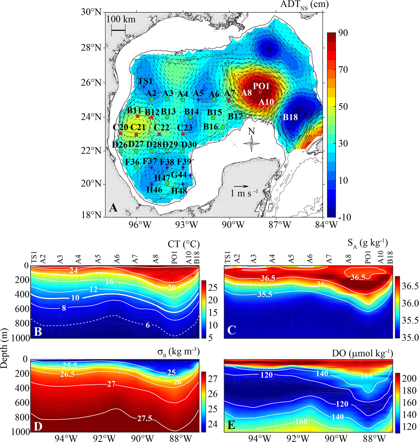
Figure 1 (A) Mean non-steric absolute dynamic topography (ADT_NS, cm) during the XIXIMI-5 cruise. The black lines correspond to the 200, 1000, and 3500 m isobaths. The blue rhombuses (), green circles (), and red squares () correspond to cyclonic (CE), no eddy (NE), and anticyclonic (AE) stations, respectively, which were classified using the nitracentric classification. The Loop Current (LC) stations are represented by white labels. The vectors show the surface geostrophic velocity currents derived from horizontal ADT_NS gradients. The spatial distribution sections of conservative and non-conservative properties obtained with CTD data for the northernmost transect include: (B) Conservative Temperature (CT, °C), (C) absolute salinity (S_A, g kg^-1) (D) potential density anomaly (σ₀, kg m^-3), and (E) dissolved oxygen (DO, µmol kg^-1).

2.2 Classification

Based on the NN profiles, the 35 stations were classified as cyclonic (CE), no eddy (NE), or anticyclonic (AE). The AE stations were further classified into two sub-groups: a sub-group of AE stations in the interior of the GM (i.e., west of 90° W) and a sub-group of stations under the influence of the recently detached LCE Poseidon. This nitracentric classification required quasi-continuous vertical profiles of NN concentrations, which were obtained from the discrete NN profiles using the PCHIP interpolation method (Fritsch and Carlson, 1980) in the same depth interval (~ 1 m) as the CTD variables (Figure S1). Interpolated NN profiles were integrated by depth to obtain the NN stock (NN_int-z) at 97 integration intervals that spanned an upper depth horizon of 15 m to varying depths from 20–500 m at 5-m increments. Based on the premise that an upward (downward) deflection of the pycnocline would yield larger (smaller) values in CEs (AEs) stations than in NE stations, for each integration depth the stations were ranked based on NN_int-z. With the ranked stations, the limits between station groups were defined based on the analysis of the standardized NN stock anomalies and box-and-whisker plots (see details in Figure S1). Statistically, we considered that the best depth to integrate NN_int-z to classify stations is the one that produces the greatest separation between groups, which was 200 m (NN_int-200).

Additionally, we analyzed hydrographic data obtained with the CTD to identify variables that could be used to obtain a similar classification of stations as the nitracentric classification (Figure S1). We explored the depths of 23 isotherms (6–28°C with 1°C intervals), Conservative Temperature (CT) and the density anomaly at 98 depths (15–500 m with 5-m intervals), and the depths of nine isopycnals (23.5–27.5 kg m^-3 with 0.5 kg m^-3 intervals). Other variables were also explored at the fluorescence maximum and DO minimum, including the NN concentration, fluorescence, absolute salinity (S_A), CT, DO, and potential density anomaly (σ₀). We also tested 98 dynamic height anomalies calculated from 15–1000 to 500–1000 m at 5-m intervals. In addition, 58 Brunt-Väisälä (B-V) frequency (15–300 m with 5-m intervals) and integral (referred to 15 m) values were used. Absolute dynamic topography and sea level anomaly (SLA) data were obtained by altimetry (http://marine.copernicus.eu/). We removed the steric components of the altimetric measures by subtracting the daily average for the entire region. To exclude high frequency variability due to wind forcing, we only considered data in regions off the continental shelf (> 200 m depth; Dukhovskoy et al., 2015; Hamilton et al., 2018). Lastly, the mixed layer depth (MLD) was calculated by the relative variance method (Huang et al., 2018) and by the segment method (Abdulla et al., 2016) from individual temperature or density profiles.

The physical variables that produced classification results similar to those of the nitracentric classification were deemed the BFVs (Figure S1). These variables were best able to reflect mesoscale effects on the vertical distribution of NN and thus facilitate NN_int-z and NN predictions. The absolute value of the Pearson correlation coefficient (|r|) was calculated between each hydrographic variable and NN_int-200, and the BFVs were identified as the variables that resulted in the highest Pearson correlation coefficients that simultaneously fulfilled the criteria of |r| ≥ 0.80 and |r| ≥ 0.90 for data with (n = 35) and without (n = 32) Poseidon stations, respectively. Six BFVs were identified: the depth of the 20°C isotherm (Z_CT20), potential density anomaly at 120 m (σ_0-Z120), Conservative Temperature at 140 m (CT_Z140), depth of the 26 kg m^-3 isopycnal (Zσ₀₂₆), integrated dynamic height between 1000–60 m (DH₆₀), and integrated Brunt-Väisälä frequency between 15–120 m (B-V_int-120).

To verify that 200 m was the best NN integration depth, that is, the integration depth that resulted in the greatest separation among station groups, |r| was plotted against the NN integration depth (Figure S2). The Pearson correlation coefficients and corresponding p-values (α = 5%) were determined for the relationships between each BFV and NN_int-z (NN_int-20,…, NN_int-500). In other words, for each station, 97 NN_int-z values were calculated (one for each integration depth). Thus, for any given integration depth, 35 and 32 NN_int values were available within our sampling grid (including or excluding Poseidon stations, respectively). For each integration depth, the absolute value of the Pearson correlation coefficient and the p-value (34 or 31 degrees of freedom) were calculated for the relationship between NN_int-z and the value of the BFV obtained for each station.

The high linear correlations (|r| ≥ 0.8, Figure S2) obtained between each BFV and the NN stock at all integration depths between ~ 100–500 m, allowed us to predict the vertical distribution of NN and NN_int-z from hydrographic variables within this depth range in stations in the interior of the GM. This was accomplished first by fitting a straight line between each BFV and each NN_int-z (Equation 1), and thus a total of 81 linear equations were obtained (one for each integration depth located every 5 m between 100 and 500 m) with their corresponding slope (β₁) and intercept (β₀) values. For example, the values of β₁ and β₀ for the equations using the depth of the 20°C isotherm as a predictor of NN_int-z [i.e., NN_int-z = β₁ (z) Z_CT20 + β₀ (z)] at z = 100, 300, and 500 m were -1.96 mmol m^-3 and 310.91 mmol m^-2, -21.49 mmol m^-3 and 5589.46 mmol m^-2, and -30.13 mmol m^-3 and 11776.78 mmol m^-2, respectively. Second, at any given sampling station, the NN stock and NN concentration can be predicted for any depth using least squares (Equations 2–3), which were obtained from the relationships of β₁ and β₀ with depth (Figure S3). Since the β₁ and β₀ obtained for each linear regression between NN_int-z and each BFV in Equation 1 are non-linear functions of depth (Figure S3), we explored second, third, and fourth degree polynomial fits in the least-squared sense. For example, β₁ and β₀ in Equation 1 were replaced with cubic polynomial fits to obtain Equation 2.

$\begin{array}{ll}N{N}_{\mathrm{int}-z,j}={\beta }_{1,j}(z)\mathrm{BF}{V}_j+{\beta }_{0,j}(z)& (1)\end{array}$

$\begin{array}{ll}N{N}_{\mathrm{int}-z,j}=(a_{1,j}{Z}^3+b_{1,j}{Z}^2+c_{1,j}Z+d_{1,j})\mathrm{BF}{V}_j+(a_{2,j}{Z}^3+b_{2,j}{Z}^2+c_{2,j}Z+d_{2,j})& (2)\end{array}$

$\begin{array}{ll}N{N}_j=(3a_{1,j}{Z}^2+2b_{1,j}Z+c_{1,j})\mathrm{BF}{V}_j+(3a_{2,j}{Z}^2+2b_{2,j}Z+c_{2,j})& (3)\end{array}$

where a₁, b₁, c₁, and d₁ are the cubic polynomial fit coefficients for the relationship between β₁ and depth, while a₂, b₂, c₂, and d₂ are the corresponding coefficients between β₀ and depth. The subscript “j” refers to each BFV. Once the degree of the polynomial was chosen to parameterize NN_int-z, the NN concentration (Equation 3) was calculated by differentiating NN_int-z (Equation 2) with respect to depth. Finally, “vertical profiles” were constructed for the NN stock values calculated with the observed/interpolated data and with the values predicted for each of the BFVs (NN_int-100, NN_int-105, …, NN_int-500). Goodness of fit was evaluated based on the mean absolute error (MAE), the root-mean-square error (RMSE), and bias (BIAS) statistical descriptors, which were calculated between the observed (interpolated) and predicted profiles (Equations 2–3) of each sampling station in the 100–500 m depth interval. For each of the BFV predictions, box plots of the RMSE, MAE, and BIAS were constructed with data for 32 stations (i.e., excluding Poseidon stations). Finally, the polynomial fit that produced the lowest RMSE, MAE, and BIAS (closest to zero) for NN and NN_int-z for each BFV was chosen.

To evaluate the ability of the parameterization to accurately predict NN profiles from other summer cruises in the deep-water region of the GM, data from 12 stations sampled during XIXIMI-4 (summer 2015) and XIXIMI-6 (summer 2017) were used to classify the stations as CE, NE, or AE using the same methodology. Additionally, to test the ability of the parameterization to accurately predict NN profiles under winter conditions, data from the 30 stations sampled during the winter cruise XIXIMI-3 (19 February to 10 March 2013) were used to classify stations as CE, NE, or AE. Data from six XIXIMI-3 stations (two CE, two NE, and two AE) were used to evaluate the ability of the parameterizations obtained with both XIXIMI-5 and XIXIMI-3. Finally, to explore the applicability of the classification methodology in an open-ocean oligotrophic region out of the GM, we analyzed stations in the eastern Caribbean Sea at CLIVAR section A22 (see Supplementary Material) where continuous CTD data and discrete nutrient data are available for three cruises carried out in summer (16-21 August 1997; 25 stations), autumn (24-29 October 2003; 24 stations), and spring (9-14 April 2012; 26 stations; https://www.ncei.noaa.gov/access/ocean-carbon-data-system/oceans/RepeatSections/ ).

As a measure of the classification accuracy, we averaged all of the interpolated NN profiles for the CE, NE, and AE groups meter by meter, and we computed the corresponding confidence intervals (CI; t-test with α = 5%). Averages were also obtained only for AE stations under the influence of the LCE Olympus (B11, B12, C21, C22), CE stations within the cyclonic eddy of the Bay of Campeche (F37, F38, F39, and H46), and NE stations (A3, A4, B13, D30, D28, and F36; Figure 1A). For the purpose of comparison, average profiles were constructed by grouping stations based on other eddy classification criteria (e.g., altimetric and hydrographic criteria), including criteria that have been recently used to regionalize the gulf (Linacre et al., 2015; Müller-Karger et al., 2015; Pasqueron de Fommervault et al., 2017; Damien et al., 2018; Hamilton et al., 2018; Lee-Sánchez et al., 2022).

3 Results

3.1 Hydrographic Samples

The LCE Poseidon detached from the LC in April 2016. As reflected in the spatial distribution of CT, DO, S_A, and σ₀, a downward deflection of the pycnocline of more than 200 m was present in the central portion of the eddy. This downward deflection was indicative of a deepening of up to ~ 1000 m of warm water with relatively higher salinity and lower density (Figures 1B–E), resulting in an increase in DO in the first 200 m of the water column (Figure 1E) and a deepening of the subsurface salinity maximum that characterizes North Atlantic Subtropical Underwater, which is commonly found between 150–230 m (Portela et al., 2018). In addition, this downward deflection resulted in a deepening (~ 600 m) of the oxygen minimum, which is indicative of the core of Tropical Atlantic Central Water and generally located between 400–600 m (Portela et al., 2018). These types of changes in eddy cores allow eddies to be easily classified based on the vertical distributions of hydrographic variables, primarily temperature and salinity.

Changes in mesoscale eddy properties and their intensity can be visualized in T-S diagrams. Figure 2 presents cascade T-S diagrams (from 10 to 200 m, ΔS_A = 0.2 g kg^-1) for all sampled stations. Notable differences in NN and temperature can be observed between stations under the influence of the LCE Poseidon (PO1, A8, and A10) and stations under the influence of the CE in the Bay of Campeche (H46, F37-F39; Figure 2A). From 10–200 m in station PO1, concentrations of 0 < NN < 2 µmol kg^-1 and relatively high temperatures throughout the profile (25 < CT < 30°C) were present, whereas ample gradients of 0 < NN < 21 µmol kg^-1 and 13 < CT < 30°C were apparent in station H46. Clearly contrasting T-S distributions were also observed between CE stations (e.g., TS1 and B18) and stations under the influence of the LCE Olympus (e.g., B11, B12, C21, and C22). However, differences between the T-S profiles were less evident among many stations, and it was at times difficult to determine which stations were under the influence of mesoscale eddies. In Figures 1, 2A, the presence of the LCE Poseidon and other mesoscale eddies is clear, and the station classification (CE, AE, and NE) is almost obvious. However, when only altimetric criteria were used (Hamilton et al., 2018; http://marine.copernicus.eu/services-portfolio/access-to-products/), stations like D26, C20, D27, and B12 could not be easily classified.

FIGURE 2

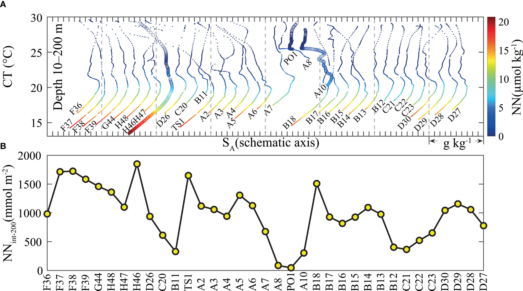
Figure 2 (A) Cascade T-S diagram (from 10 to 200 m, ΔS_A = 0.2 g kg^-1) for all sampling stations, where the background color indicates the nitrate + nitrite (NN, µmol kg^-1) concentration. The profiles of stations H46, PO1, and A10 are highlighted with circular markers. (B) Depth-integrated NN between the surface and 200 m (NN_int-200, mmol m^-2) of profiles interpolated by the PCHIP method.

3.2 Nitracentric Classification

The reconstruction of vertical NN profiles allowed for the NN stock to be calculated at depths different from those of the discrete samples, which was necessary to identify the depth at which the integrated concentration produced the best nitracentric classification. Although no discrete samples were collected at 200 m, NN_int-200 was best able to reflect the effects of mesoscale eddies on NN availability in the water column (Figure 2B). The highest NN stock values at 200 m (> 1500 mmol m^-2) were observed in the CE stations in the Bay of Campeche (F37–F39 and H46), the station under the influence of the CE that strangled the LC (B18), and station TS1. In contrast, the lowest NN_int-200 values (< 500 mmol m^-2) were present in stations under the influence of the anticyclonic LCEs Olympus (B11, B12, C21, C22) and Poseidon (PO1, A8, A10).

The station ranking based on the NN stock was, in general, similar for all integration intervals from 15–150, 15–165, and so on up to 15–250 m depth (NN_int-150, …, NN_int-250), thus resulting in the same station grouping and allowing for different mesoscale eddies to be distinguished in terms of NN availability in surface waters (Figure 3A). It is important to note that no stations switched groups when their NN_int-z values were ranked within integration intervals with upper limits between 160–470 m (i.e.: NN_int-160, …, NN_int-470). In terms of the NN stock, the best station separation was obtained when NN was integrated from 15–200 m (NN_int-200, Figures 3A, C–E), as this resulted in the greatest separation between groups and the smallest variance within each group. This was due to the low variability of NN_int-z in the NE stations, which resulted in a low slope (thick black line, Figure 3A) and low amplitude of the data centered in box-and-whisker plots (Figures 3C–E).

FIGURE 3

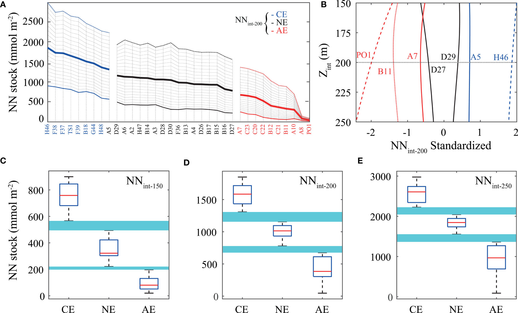
Figure 3 (A) Nitrate + nitrite (NN) integrated in the depth intervals of 15–150, 15–155, and so on up to 15–250 m with stations ranked according to NN_int-200 (NN integrated between surface and 200 m, mmol m^-2). The uppermost and lowermost lines correspond to NN_int-250 and NN_int-150, respectively, while the thicker, colored lines correspond to NN_int-200. (B) Standardized NN_int-z for stations located within the group classification limits for the same integration intervals as in (A). Z_int indicates the upper depth limit of the NN integral. The blue, black, and red lines correspond to the cyclonic (CE), no eddy (NE), and anticyclonic (AE) groups, respectively. The red dotted line indicates the boundary between the AE and Poseidon stations, while the blue and red dashed lines correspond to the stations H46 and PO1, respectively. Box plots of (C) NN_int-150 (mmol m^-2), (D) NN_int-200 (mmol m^-2), and (E) NN_int-250 (mmol m^-2) for all sampled stations. The cyan regions correspond to the NN_int-z intervals that separate the CE (n = 9), NE (n = 15–16), and AE (n = 9–10) groups. The red line inside each box is the median of the data. The standardization of NN_int-z was done for each depth integration interval using the equation: standardized (NN_int-z) = [NN_int-z - mean (NN_int-z)]/SD (NN_int-z).

The limits between station groups were defined based on standardized NN stock anomalies for stations within each integration interval, which allowed for the station classification based on NN_int-200 to be validated (Figure 3B). In the NN integration intervals of 15–150, 15–155, and so on up to 15–250 m, standardized anomalies greater than 0.6, those between -0.40 and 0.6, and those less than -0.40 were used to classify stations into CE, NE, and AE groups, respectively (Figure 3B). For the integration limit of 15–200 m, 9 CE stations (NN_int-200 ≥ 1,300 mmol m^-2), 16 NE stations (770 < NN_int-200 < 1,150 mmol m^-2), and 10 AE stations (NN_int-200 < 770 mmol m^-2) were identified (Figures 3A, D; Table S1). The mean NN_int-200 value for stations under the influence of the LCE Poseidon (NN_int-200 < 145 mmol m^-2) reflected the effect of a marked downward deflection of the nitracline in the station located in the core of the eddy (PO1; ~ 46 mmol m^-2). A notable difference was observed between the mean values of the AE stations in the interior of the GM (~ 510 mmol m^-2) and the CE stations (~ 1,570 mmol m^-2), although the greatest difference was observed between stations H46 and PO1, with the NN_int-200 value of station H46 (~ 1,850 mmol m^-2) being 40-fold higher than that of PO1.

The results of the nitracentric classification indicated that NN_int-200 results in the best station classification, considering the effects of mesoscale eddies (or the absence thereof). For this reason, NN_int-200 was contrasted with hydrographic variables to determine those best able to represent the effects of mesoscale eddies on the vertical distribution of NN in the GM.

3.3 Hydrographic Classification

3.3.1 Selection of the Best Fit Variables

Linear regressions were used to compare each hydrographic variable with NN_int-200, and the variables that resulted in the highest Pearson correlation coefficients (|r_i|) were selected. The variables that simultaneously fulfilled the criteria of |r| ≥ 0.8 and |r| ≥ 0.9 for station groups that included stations under the influence of the LCE Poseidon and those that did not are summarized in Table 1. Except in the case of B-V_int-120, the inclusion of the Poseidon stations in the BFV analysis lowered the resulting correlation coefficients, although the overall trends were preserved. Based on the intervals with the best correlations between each BFV and NN_int-200, six variables were selected that yielded the highest correlation coefficients (Table 1): 1) the depth of the 20°C isotherm (Z_CT20), 2) CT at 140 m depth (CT_Z140), 3) the potential density anomaly at 120 m depth (σ_0-Z120), 4) the depth of the 26 kg m^-3 isopycnal (Z_σ026), 5) integrated dynamic height between 1000–60 m (DH₆₀), and 6) the integrated B-V frequency between 15–120 m (B-V_int-120). Table 1 also contains the “best intervals” of the values of each BFV that can be used with a high degree of confidence to represent the variability in NN_int-200 due to mesoscale eddy activity. Although ADT was also found to be associated with NN_int-200, particularly when the Poseidon stations were excluded (|r| = 0.86), it did not meet the criteria for BFV selection.

TABLE 1

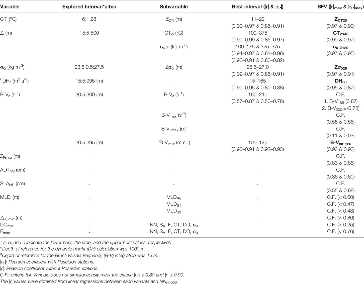
Table 1 Variables considered in the classification of stations into cyclonic (CE), no eddy (NE), and anticyclonic (AE) groups. .

To evaluate the consistency of the BFVs regarding their equivalency to NN_int-z in order to classify stations within a broader NN integration interval and not only at 200 m, a new linear model was fitted between each selected BFV (Table 1) and NN_int-z for all integration intervals between 15–500 m. The |r| coefficients (Figures S2A, B) and p-values between the selected BFVs and NN_int-z were calculated (α = 5%; n = 35 and n = 32 when the Poseidon stations were included and excluded, respectively; Figures S2C, D). An exponential increase was observed in both correlation coefficients with the integration of NN between 15–60 m, and a high linear correlation (|r| ≥ 0.8) was observed after 100 m (Figures S2A, B). The differences between coefficients were due to the variability produced by the stations under the influence of Poseidon that resulted in, among other things, lower NN_int-200 values (~ 400 mmol m^-2) when compared to the average of the group that did not contain these stations (~ 509 mmol m^-2; Table S1). The p-value confirmed the high linear correlation between the BFVs and NN_int-z after 65 m (Figures S2C, D). This indicates that it is possible to use the BFVs as classifying variables and possible predictors of NN_int-z, especially for integration depths greater than 100 m and when Poseidon stations are not included.

3.3.2. Analysis of the Best Classifying Variables

The variables that presented the highest correlations with NN_int-200 were selected as the BFVs and used to classify stations. However, high correlation coefficients were obtained within a range of values for the hydrographic variables referred to as the “best interval” (Table 1). For example, when the Poseidon stations were excluded, the depth of the 20°C isotherm (Z_CT20) presented the highest correlation with NN_int-200 (0.97), although the depths of all the isotherms in the range of 11–22°C also presented relatively high values (|r| = 0.90–0.97). It should be noted that the depth of the 6°C isotherm, which has been frequently used to identify stations under the influence of mesoscale eddies in the GM (Bunge et al., 2002; Pasqueron de Fommervault et al., 2017; Hamilton et al., 2018), was associated rather poorly with NN_int-200 (|r| < 0.60). In addition, the temperature at 140 m was highly correlated with NN_int-200 (|r| = 0.99), although it should be noted that the temperatures corresponding to all depths between 100–375 m also presented high correlations (|r| = 0.90–0.99; Table 1).

To explore BFV trends with regard to the station classification based on NN_int-200, the values of the hydrographic variables in the best interval were plotted against the station rankings [i.e., highest (station H46) to lowest (station PO1)] with regard to NN_int-200 (Figure 4). For cases in which the station ranking based on the value of the hydrographic variable was different from the ranking based on NN_int-200, the corresponding curves showed peaks. This indicates that if BFVs are used to predict NN and/or the NN stock, the resulting values could be either over- or underestimated in some stations. An example is illustrated by station B18, which was under the influence of a CE that strangled the LC and resulted in the generation of the LCE Poseidon. The NN_int-200 ranking placed station B18 in sixth place in the CE group, although the hydrographic information indicated that this station was under the greatest CE influence at the time of sampling. This was probably due to the fact that the CE influencing station B18 consisted of relatively young subsurface waters from the northwestern region of the GM with low NN content. In contrast, station H46 was sampled in the southern waters of the GM, which have relatively long residence times within the gulf and thus higher accumulated NN concentrations due to respiration. This may also explain the peaks observed in stations B17 (NE), H48 (CE), and A7 (AE), which shifted to the left (A7) or right (B17 and H48) of the group order according to the hydrographic classification (see σ_0-Z120 and CT_Z140, Figures 4C, D).

FIGURE 4

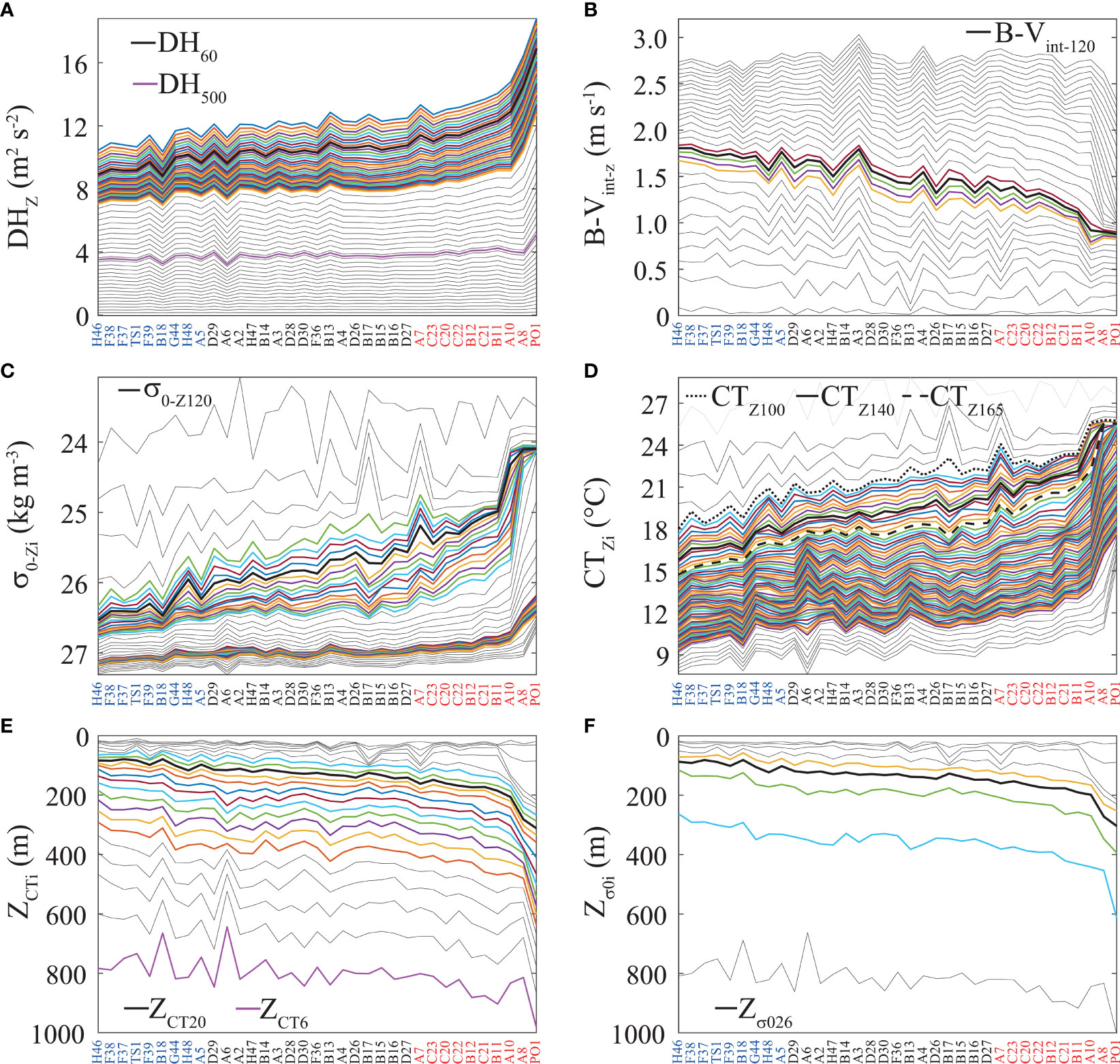
Figure 4 Best fit variables (BFVs) and the intervals explored for each variable. (A) Dynamic height (DH_z, m² s^-2) anomaly integrated from 1000–15, 1000–20, and so on up to 1000–995 m. (B) Brunt-Väisälä frequency integrated (B-V_int-z, m s^-1) over 15–20, 15–25, and so on up to 15–300 m. (C) Potential density anomaly (σ_0-Zi, kg m^-3) and (D) Conservative Temperature (CT_Zi, °C) in depths of 15, 20, 25, and so on up to 500 m. (E) Depth of the 6, 7, and so on up to 28°C isotherms (Z_CTi, m). (F) Depth of the 23.5, 24.0, and so on up to 27.5 kg m^-3 isopycnals (Z_σ0i, m). The colored lines represent the best fit intervals for each BFV and preserve the interval separation (Table 1). To facilitate visualization, the thin black lines of some BFVs were plotted with different separations at the intervals defined in Table 1 with separations of (A) 30 m, (B) 10 m, (C) 20 m, and (D) 20 m. The thick black line is the BFV. The magenta lines in Panels (A, E) correspond to DH₅₀₀ and Z_CT6, respectively. The stations labeled blue, black, and red correspond to the cyclonic (CE), no eddy (NE), and anticyclonic (AE) groups, respectively. The stations were ranked based on NN_int-200 from highest (H46) to lowest (PO1). Note that in Panels (C, E, F), the ordinate axis is reversed.

Choosing a classification criterion outside the best interval could result in a less suitable classification for analyzing the effects of mesoscale eddies on biogeochemical variables, such as NN. For example, according to the depth of the 6°C isotherm (magenta line in Figure 4E), station A6 was under the greatest CE influence, whereas the BFVs classified it as an NE station. Additionally, station A8 was classified in the NE group, although it was located within the intense LCE Poseidon (Figure 4E). On the other hand, five out of six stations located within the cyclonic eddy of the Bay of Campeche were classified in the NE group (H46, H48, G44, F39, and F38), of which H46 and F38 had the highest NN_int-200 (1850 and 1725 mmol m^-2, respectively). The station classification based on the depth of the 6°C isotherm resulted in average NN profiles with overlapping confidence intervals (see section 3.4).

Peaks in the values of the hydrographic variables in some stations (Figure 4) indicate changes in the relationships between these variables and NN_int-200 when compared to those of similar classifications. In some cases, the hydrographic variables presented opposing peaks at different densities, which may reflect the presence of subsurface hydrographic features, such as lens-shaped structures. For example, in the NE group, stations B17 (σ₀ < 26.5 kg m^-3, Figure 4C; CT < 18°C, Figure 4D) and A6 (σ₀ > 26.5 kg m^-3, Figure 4C; CT > 17°C, Figure 4D) appear to have typical characteristics of intra-thermocline lenses or subsurface-intensified eddies (Assassi et al., 2016). The isopycnals/isotherms in these stations showed CE-type behavior (termed “thinny” by McGillicuddy, 2015) in which the seasonal (permanent) thermocline is displaced downwards (upwards), producing a concave lens (Figures 4E–F). These lenses were clearly detectable in Figures 4C, D, although they were also observed in Figures 4E, F (200–800 m in A6 and 15–200 m in B17) with the depth isolines in opposing directions. The presence of these lenses could alter the classification of a station and result in it being assigned to another group if a suitable hydrographic variable is not selected as the separation criterion. For example, if CT at 100 m or 165 m is chosen as a BFV (both located within the best interval, Table 1), station B17 (NE) would be classified as being under the influence of either a strong AE or weak CE, respectively (Figure 4D).

3.3.3 Contour Maps of BFVs, NN Stock, and Sea Level Anomalies

The BFV contour maps reflect both the highly correlated linear relationships with NN_int-200 and mesoscale eddy effects (Figures 5A–G). Among the BFVs, B-V_int-120 and σ_0-Z120 showed direct linear relationships with the NN stock at 200 m, while the others presented inverse linear relationships. The BFVs reflected the presence of the LCEs Poseidon (A8, A10, and PO1) and Olympus (B11, B12, C21, and C22) and the CEs in the Bay of Campeche (F37, F38, and H46) and in stations TS1, B18, and A5. The largest differences between NN_int-200 and the BFV maps were observed with the B-V_int-120 map in stations A4, A5, A6, and B14 (Figure 5G). The NE stations were distributed throughout the study area and presented similar BFV and NN_int-200 values (Figures 3A–D), reflecting the fact that all of these stations showed similar NN profiles between 15–200 m despite being separated by hundreds of kilometers, as can be observed from the low variability in the CI of the NE group in Figures 6A, C, D, F.

FIGURE 5

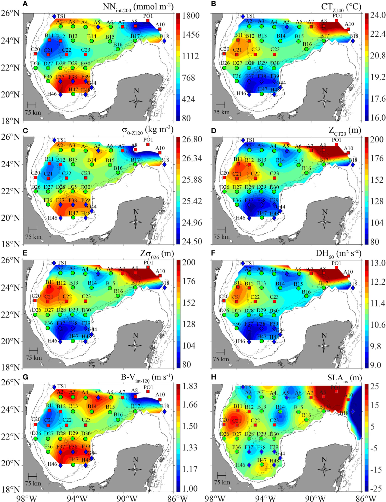
Figure 5 Contour maps of (A) depth-integrated nitrate + nitrite (NN) between surface and 200 m (NN_int-200, mmol m^-2), (B) Conservative Temperature at 140 m (CT_Z140, °C), (C) potential density anomaly at 120 m (σ_0-Z120, kg m^-3), (D) depth of the 20°C isotherm (Z_CT20, m), (E) depth of the 26 kg m^-3 isopycnal (Zσ₀₂₆, m), (F) integrated dynamic height between 1000–60 m (DH₆₀, m² s^-2), (G) the integrated Brunt-Väisälä frequency between 15–120 m (B-V_int-120, m s^-1), and (H) non-steric SLA during the cruise (cm). The blue rhombuses (), green circles (), and red squares () correspond to cyclonic (CE), no eddy (NE), and anticyclonic (AE) stations, respectively.

FIGURE 6

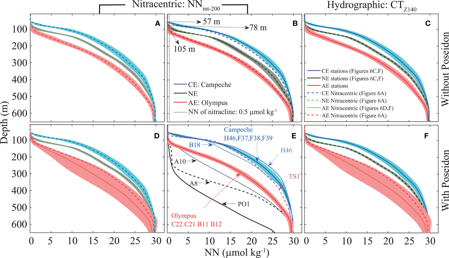
Figure 6 Average of the nitrate + nitrite (NN, µmol kg^-1) depth profiles with 95% confidence intervals (CIs) for cyclonic (CE; blue-cyan), no eddy (NE; black-green), and anticyclonic (AE; red-pink) groups obtained by both nitracentric (left and central panels) and hydrographic (right panel) classifications without (A–C) and with (D–F) the Poseidon stations. (B) Average of the nitrate + nitrite (NN) depth profiles (± SD) for the Olympus stations (B11-B12, C20-C22; red), some Campeche stations (F37-F39, and H46; blue), and some NE stations (A3-A4, B13, D28, D30, and F36; black). (E) The same CE and AE groups as in (B) but including the vertical profiles of the Poseidon stations and the three stations of the CE group (H46, B18, and TS1). The thick blue, black, and red lines are the means of the CE, NE, and AE groups, respectively. In (A–D, F), the blue (CE), green (NE), and red (AE) dashed lines are the NN means in (A). The dotted red line is the NN mean of the AE group in (D). The values in panel (B) indicate the nitracline depth, which was defined as the depth at which a concentration of 0.5 µmol kg^-1 is observed (Cianca et al., 2007; Linacre et al., 2019).

With non-steric SLA (Figure 5H) and non-steric ADT (Figure 1A) contour maps, the stations under the influence of the most dominant eddies, including the anticyclonic LCEs Poseidon and Olympus and the CE in the Bay of Campeche, are clearly visible. However, some stations (B14, A2, and C23 in the SLA map and F39, G44, H48, D26, and D29 in the ADT map) were difficult to classify or were classified in different groups than those based on the BFV classification.

3.4 Average NN Profiles

Similar average vertical profiles were obtained with the nitracentric and hydrographic classifications, either including or excluding the Poseidon stations (Figures 6A, C, D, F). In general, the mean NN values in the CE, NE, and AE groups coincided at ~ 650 m (Figures 6A–D, F). Both the nitracentric and hydrographic classifications (see the classification based on CT_Z140 in Figures 6C, F, which is similar to the classifications based on other BFVs) resulted in the separation of the three groups along the profile up to 500 m. At this depth, the limits of the 95% CIs of the NE and CE groups overlapped (Figures 6C, F). The CIs of the AE and NE groups and those of the AE and CE groups overlapped after 560 m when the Poseidon stations were not included (Figures 6A, C). The inclusion of the Poseidon stations (Figures 6D, F) notably modified the average NN profiles in the AE group due to great differences in the biogeochemical and hydrographic properties of the water column of the recently detached LCE (Figures 1B–E). When the stations of the Campeche CE, the Olympus AE, and the central region of the GM were contrasted, a complete separation of the CIs was observed down to ~ 570 m (Figure 6E). Within the depth interval of the euphotic layer (≤ 150 m; Linacre et al., 2019), the differences in mean NN values between CE and AE stations were ~ 1.0 µmol kg^-1 at 60 m, ~ 8.5 µmol kg^-1 at 100 m, and ~ 11.5 µmol kg^-1 at 150 m (Figure 6B). Even when considering the average profiles for the total set of stations (excluding those of the LCE Poseidon), the difference in NN in the euphotic layer between the CE and AE groups was clear, with values of ~ 0.5 µmol kg^-1 at 60 m, ~ 7.6 µmol kg^-1 at 100 m, and ~ 9.7 µmol kg^-1 at 150 m (Figure 6E).

The stations showing the greatest contrast were PO1 (the station under the greatest influence of anticyclonic circulation) and H46 (the station under the greatest influence of cyclonic circulation). These stations showed differences in mean NN values that increased from ~ 9.1 to ~ 24.2 µmol kg^-1 between 100–300 m, respectively. Another marked contrast in NN was evident below 100 m between the Poseidon stations and the average profile of the Olympus stations (Figure 6E), with differences at 300 m of 4.8, 13.1, and 16.0 µmol kg^-1 with respect to stations A10, A8, and PO1, respectively. On the other hand, station B18, which was located within an intense CE, presented lower concentrations of NN between 100–400 m compared to those of station H46, with a maximum difference of ~ 4 µmol kg^-1 around 150 m (Figure 6E). The strong effect of mesoscale eddies is also noticeable in the nitracline (~ 0.5 µmol kg^-1) depth, which was observed at 50 m in the Campeche CE and below 100 m in the LCEs Olympus and Poseidon.

3.5 Parameterization of NN and NN_int-z

Second, third, and fourth degree polynomials were used to predict the slopes (β₁) and intercepts (β₀; Equations 1–3) of the linear regressions obtained between each BFV and NN_int-z for each meter of depth between 100–500 m. In this way, the NN stock was predicted (Equation 2; third degree polynomial), and NN was subsequently obtained by differentiating with respect to depth (Equation 3). The results showed that the three polynomial fits were adequately able to predict the NN stock (Figure 7), although the second degree polynomial produced straight lines with depth while the observed profile indicated curvature. The second degree polynomial prediction overestimated the NN values throughout the depth interval (100–500 m) of the calculation, producing MAE and RMSE medians that were greater than those obtained with the third and fourth degree polynomial fits (> 1.5 µmol kg^-1 vs < 1 µmol kg^-1, respectively; Figures S4A–L). On the other hand, the MAEs and RMSEs of the BFVs for the third and fourth degree polynomials were similar for both NN and NN_int-z (Figures S4A–L). For simplicity, the third degree polynomial fit was chosen for the predictions (Table S3). When comparing the BFVs, it was found that the variability and medians of the MAEs and RMSEs for NN (< 0.7 and < 1 µmol kg^-1, respectively) and NN_int-z (< 140 mmol m^-2) were similar for most BFVs, with the exception of B-V_int-120. This BFV produced the largest errors and dispersion in all polynomial fits (MAE > 0.7, RMSE > 0.7 µmol kg^-1 and MAE, RMSE > 140 mmol m^-2 for NN and NN_int-z, respectively). The analysis of the BIAS (Figures S4M–R) showed similar results as those for MAE and RMSE, indicating that NN and NN stock predictions for the 100–500 m depth interval are similar with the three polynomial parameterizations for all of the BFVs (medians ~ 0 mmol m^-2). However, the second degree polynomial parameterization resulted in larger bias for NN (medians > 1.5 µmol kg^-1) when compared with the bias observed with the third and fourth degree parameterizations (medians ~ 0 µmol kg^-1). BIAS also shows that B-V_int-120 is the BFV with the largest deviations in the NN and NN_int-z predictions (Figures S4M–R).

FIGURE 7

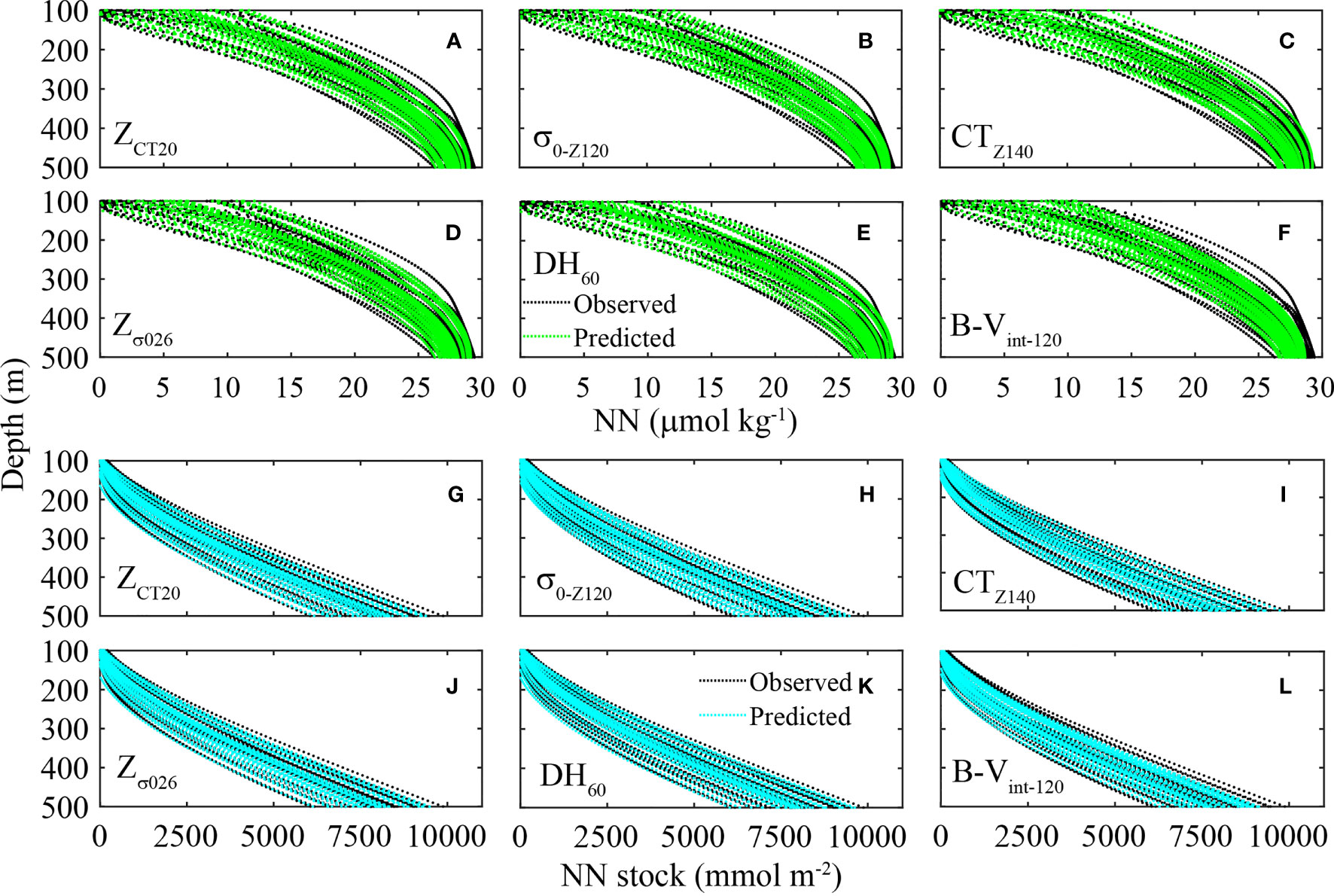
Figure 7 Observed (black dots, ) and predicted (green dots , and cyan dots) NN values (µmol kg^-1) in the interval of 100–500 m (A–F) and the NN stock (mmol m^-2) (G–L) using the third degree polynomial fit (Equations 1–3) for (A, G) the depth of the 20°C isotherm (Z_CT20, m), (B, H) potential density anomaly at 120 m (σ_0-Z120, kg m^-3), (C, I) Conservative Temperature at 140 m (CT_Z140, °C), (D, J) depth of the 26 kg m^-3 isopycnal (Zσ₀₂₆, m), (E, K) integrated dynamic height between 1000–60 m (DH₆₀, m² s^-2), and (F, L) the integrated Brunt-Väisälä frequency between 15–120 m (B-V_int-120, m s^-1) without Poseidon stations.

In order to compare the ability of the fits to predict NN and the NN stock, the predicted profiles using the third degree polynomial were graphed together with the observed and PCHIP-interpolated data for all BFVs in the 100–500 m interval. Figure 7 shows that with this polynomial fit, NN and the NN stock can be correctly predicted with each BFV for each station, and it is possible to represent the horizontal and vertical variability (100–500 m) in these biogeochemical variables within the GM. In Figure 7, it is apparent that the third degree polynomial fit adequately represents the rise or downward deflection of the NN maximum (~ 30 µmol kg^-1) due to the influence of mesoscale eddies in some stations. However, predictions based on each BFV with the third degree polynomial resulted in negative values of NN for the AE group between 100–125 m, and these negative data were replaced with a value of 0 µmol kg^-1 in Figures 8B–G, according to the NN concentration values observed for the AE stations as shown in Figure 6. From 100–125 m, the largest deviations of the predicted NN values from the observed values were detected, resulting in underestimates of 2.5 ± 0.1 µmol kg^-1 and 1.0 ± 0.4 µmol kg^-1 in NE and CE stations, respectively, and overestimations of 0.4 ± 0.1 µmol kg^-1 in AE stations based on the average for the six BFVs. In addition, below 125 m, the predicted and observed average NN values for the three station groupings practically coincided (Figure 8), producing the narrowest 95% CIs in the NE group, with the exception of B-V_int-120 (Figure 8G).

FIGURE 8

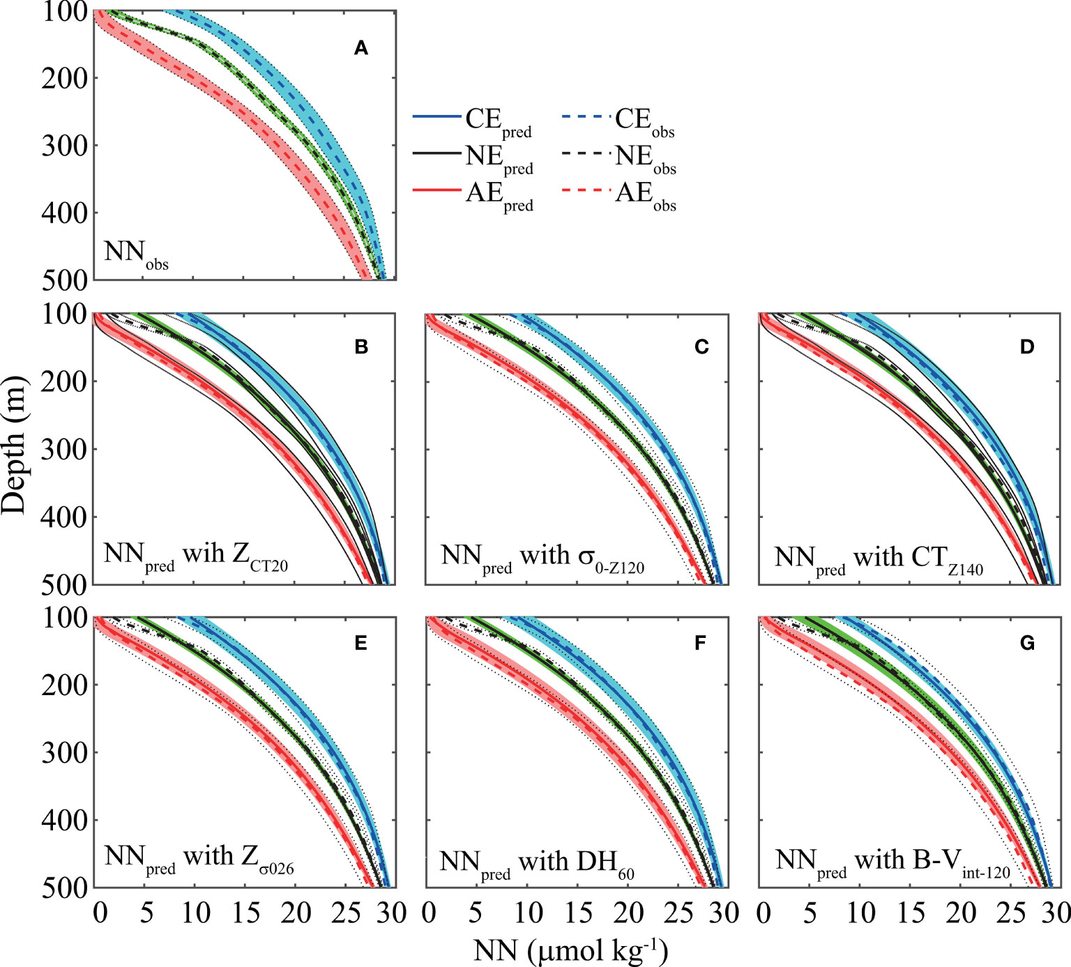
Figure 8 Average of the nitrate + nitrite (NN, µmol kg^-1) depth profiles with 95% confidence intervals (CIs) for cyclonic (CE; blue-cyan), no eddy (NE; black-green), and anticyclonic (AE; red-pink) groups without Poseidon stations. (A) NN observed and predicted (µmol kg^-1) with cubic polynomial fits for (B) the depth of the 20°C isotherm (Z_CT20, m), (C) potential density anomaly at 120 m (σ_0-Z120, kg m^-3), (D) Conservative Temperature at 140 m (CT_Z140, °C), (E) depth of the 26 kg m^-3 isopycnal (Zσ₀₂₆, m), (F) integrated dynamic height between 1000–60 m (DH₆₀, m² s^-2), and (G) the integrated Brunt-Väisälä frequency between 15–120 m (B-V_int-120, m s^-1). The blue, black, and red solid (dashed) lines correspond to the predicted (observed) average NN for the CE, NE, and AE groups, respectively. Black dotted lines correspond to ± 1 standard deviation around the observed mean of NN (Panel A). Some (~3%) predicted NN values for the AE group were negative around 100–125 m (mean ~107 m) and were replaced with 0 µmol kg^-1.

Moreover, the ability to predict NN profiles in the deep-water region of the GM was tested by employing data from 18 stations selected from the XIXIMI-4 (summer 2015), XIXIMI-6 (summer 2017), and XIXIMI-3 (winter 2013) cruises. These stations were selected from previously classified groups to include two CE stations, two NE stations, and two AE stations for each campaign. The parameterizations obtained with data from XIXIMI-5 correctly predicted the NN concentrations between 100–500 m for the summer cruises (average RMSEs 1.7 ± 0.8 and 1.0 ± 0.4 µmol kg^-1 for B-V_int-120 and for the remaining BFVs, respectively; Figures S5A, B). Furthermore, in summer cruises, lower RMSE values were obtained for CE stations with Z_CT20, CT_Z140, and Zσ₀₂₆, while the largest deviations were also obtained with B-V_int-120, particularly for the CE stations of XIXIMI-4 (2.4 µmol kg^-1), and in general for the NE (1.7 µmol kg^-1) and AE (2.0 µmol kg^-1) stations of both XIXIMI-4 and XIXIMI-6, which was more evident in the interval of ~100–120 m. However, the summer parameterizations underestimated the NN concentrations of the XIXIMI-3 winter cruise, although mostly with predictions based on the B-V_int-120 (average RMSE 9.3 ± 2.0 µmol kg^-1) while less underestimation was observed with the other BFVs (average RMSE 1.5 ± 0.5 µmol kg^-1; Figure S5C). Third degree parameterizations were also obtained for winter conditions (Table S3) using the XIXIMI-3 cruise data, and the observed and predicted NN vertical profiles are shown in Figure S5C for some of the CE, NE, and AE stations of this cruise. The winter parameterizations improved the predictions of winter NN profiles when compared with the summer parameterizations, regardless of the BFV used for the prediction (see red line in Figure S5C showing a mean RMSE of 1.1 ± 0.5 µmol kg^-1 obtained for the six stations and the six BFVs).

4 Discussion

In this study, we used the NN stock to group stations based on the effects of mesoscale eddies, a process that we call the nitracentric classification. This classification produced better separation between CE, NE, and AE stations compared to station groupings based on other classification criteria previously used in the GM. In addition, the NN stock integrated to 200 m showed high linear correlation with the hydrographic variables that we call BFVs, including Z_CT20, Z_σ026, σ_0-Z120, CT_Z140, DH₆₀, and B-V_int-120. These variables were used to obtain empirical expressions that allowed NN_int-z and vertical profiles of NN to be predicted between 100–500 m based solely on hydrographic measurements. With this methodology, the influence of mesoscale eddies on the spatial variability observed in NN_int-z and the measured profiles of NN can be adequately captured.

4.1 Nitracentric and Hydrographic Classifications

When integrated from the surface to 135–500 m depth, NN_int-z allowed for all but one of the oceanographic stations of the XIXIMI-5 campaign to be unambiguously classified into CE, AE, and NE groups. The greatest separation between station groupings was observed with the NN stock at 200 m with intervals for CE, NE, AE, and Poseidon stations of > 1,300, 770–1,300, 310–770, and < 310 mmol m^-2, respectively (Table S2). Previous studies in the gulf and in other oligotrophic areas have also observed noticeable differences in nutrient concentrations between eddy types (Biggs and Müller-Karger, 1994; Huang and Xu, 2018; Barone et al., 2019) as discussed below. Our classification resulted in clear differences in NN concentrations in intermediate waters between eddy types observed up to 600 m (Figure 6). As indicated by the nitracline depth (defined as the depth where NN = 0.5 µmol kg^-1; Cianca et al., 2007; Linacre et al., 2019), NN depletion was found at ~ 78 m in the NE group, 57 m in the CE group, and 105 m in the AE group (and up to 203 m in the core of Poseidon). The average displacement of ± 25 m around the mean depth of the nitracline under background conditions has important biogeochemical implications, namely that CEs inject nutrients into the mid layer of the euphotic zone (50–80 m) while AEs deepen NN-depleted water towards the base of this zone. As a result, the chlorophyll concentration at the deep chlorophyll maximum increases in CEs, reflecting enhanced primary production, whereas AEs show the opposite effects (Biggs and Müller-Karger, 1994; Pasqueron de Fommervault et al., 2017).

Given that the depth intervals where the BFVs are located within the upper permanent thermocline, where the nitracline is also found, the BFVs were effective in classifying stations based on the influence of mesoscale eddies and adequately reflect their modulation of NN in the upper layer of the GM (Figure 9). Apparently, the selected BFVs are sensitive to the intense baroclinic flows that characterize the eddy edges (Biggs and Müller-Karger, 1994) and produce clearly delineated group limits when compared to other classification criteria. Two of the selected BFVs were the depths of the 20°C isotherm and 26 kg m^-3 isopycnal for which the classification intervals were < 110 m for CE stations, 110–150 m for NE stations, 150–200 m for AE stations, and > 200 m for Poseidon stations (Table S2). Although Z_CT20 and Z_σ026 presented maximum linear correlations with NN_int-200, the depths of all of the isotherms from 11–22 °C and all of the isopycnals from 25.5–27.0 kg m^-3 also presented high correlations (Table 1). In previous studies of the GM, the depths of different isotherms located within the permanent thermocline have been used to identify mesoscale eddies, such as the study by Durán-Campos et al. (2017) that employed Z_CT15 and Z_CT18.5 in the Bay of Campeche and the study by Biggs and Müller-Karger (1994) that used Z_CT14 in the western gulf. It is worth noting that our classification intervals for Z_σ026 agree with outputs from the HYCOM numerical model in the GM reported by Brokaw et al. (2020; see their Figures 6, 7), where CEs showed Z_σ026 ~ 60–120 m and AEs showed Z_σ026 ~ 120–250 m. While Z_σ026 showed the highest correlation with NN_int-200, Z_σ025.5 was also highly correlated. The use of Z_σ025.5 produces a similar classification to that of the BFVs and has the advantage of having been used by other authors as a proxy for the depth of the nitracline and its relationship to mesoscale eddies (Linacre et al., 2015; Pasqueron de Fommervault et al., 2017). Our results indicate that the potential density anomaly and CT along the 120 m (σ_0-Z120) and 140 m (CT_Z140) isobaths, respectively, are also good indicators of mesoscale eddies, and they are informative in terms of the presence of water masses at these depths. The σ_0-Z120 classification intervals were > 26.0, 25.5–26.0, 25.0–25.5, and < 25.0 kg m^-3 for CEs, NEs, AEs, and Poseidon stations (Table S2), which correspond primarily to Gulf Common Water, Tropical Atlantic Central Water, Caribbean Surface Water remnant, and Subtropical Underwater, respectively (Cervantes-Díaz et al., 2022). On the other hand, the group intervals for CT_Z140 were < 18.2°C for CE, 18.2–20.2°C for NE, 20.2–24.0°C for AE, and > 24.0°C for Poseidon stations (Table S2), indicating that groups at this depth are mostly composed of the same water masses as those seen at 120 m, except for AE stations that show evidence of contributions of Gulf Common Water within the ageing LCE Olympus.

FIGURE 9

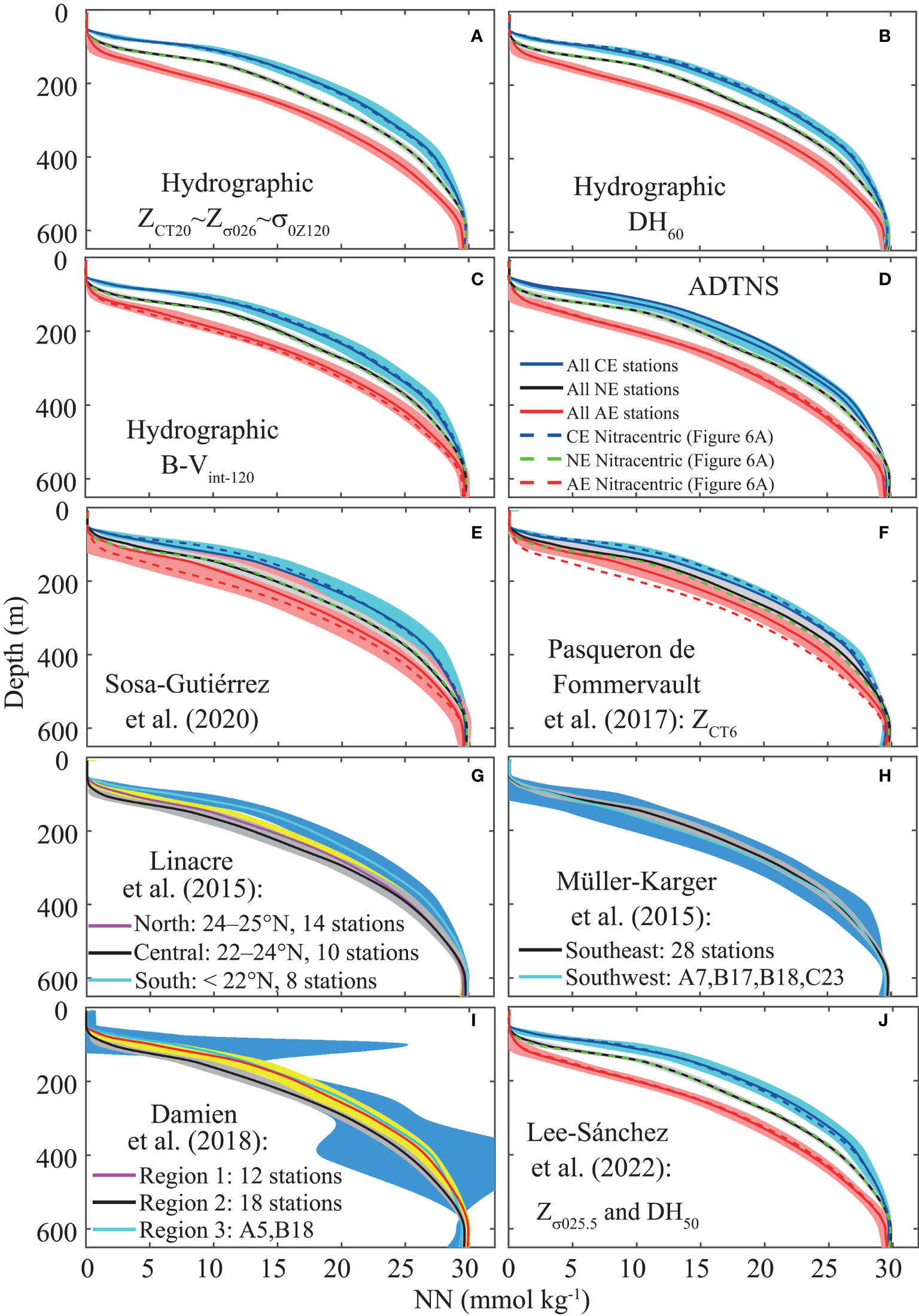
Figure 9 Average of the nitrate + nitrite (NN, µmol kg^-1) depth profiles with 95% confidence intervals (CIs) for cyclonic (CE; light blue), no eddy (NE; black), and anticyclonic (AE; red) groups obtained by (A–C) the hydrographic classification and (D) non-steric absolute dynamic topography (ADT_NS, cm). (E, F) Average NN (µmol kg^-1) profiles with CIs for the classification of mesoscale eddies based on the eddy identification criteria used by Sosa-Gutiérrez et al. (2020) and Pasqueron de Fommervault et al. (2017), respectively. (G–J) Average NN (µmol kg^-1) profiles for the geographical classifications reported by Linacre et al. (2015); Müller-Karger et al. (2015); Damien et al. (2018), and Lee-Sánchez et al. (2022), respectively. The color shaded areas correspond to CIs. The thick lines are the NN means for each group. The dashed lines are the means of the nitracentric classification (Figure 6A). The Poseidon stations were not included in the figures.

Dynamic height (DH) can be used to represent geostrophic circulation in the upper ocean (Hamilton et al., 2018). In our study, DH with an upper integration limit of 60 m (DH₆₀) was one of the selected BFVs with classification intervals of < 10.2 m² s^-2 for CE, 10.2–11.0 m² s^-2 for NE, 11.0–12.8 m² s^-2 for AE, and > 12.8 m² s^-2 for Poseidon stations (Table S2). However, DH with upper limits between 15 and 165 m also showed high correlations with the NN stock (Table 1). Although DH₆₀ has not been used in previous studies to identify eddies in the GM, Hamilton et al. (2018) reported that DH₅₀ is highly associated with SSH (> 0.91), a variable routinely used to identify mesoscale eddies. Based on this association, Hamilton et al. (2018) reported that DH₅₀ values > 14.3 and < 9.5 m² s^-2 were characteristic of AE and CE stations, respectively. In our study, DH₅₀ was also highly correlated with non-steric ADT (r ~ 0.92), but the intervals to classify CE, NE, AE, and Poseidon stations were better defined as < 10.5, 10.5–11.3, 11.3–12.7, and > 12.7 m² s^-2, respectively (Table S2). When applying Hamilton et al. (2018) intervals to our data, only two stations are classified as AE (Poseidon’s core: A8, PO1) while none of the Olympus stations are classified into this group. Furthermore, station A10 within Poseidon is classified as NE. Clearly the 14.3 m² s^-2 limit excludes stations in dissipating and even in recently released LCEs, while these stations are correctly classified as AE using our limits. Similarly, with Hamilton et al. (2018) criteria, only four stations are classified as CE (B18, TS1, H46, and F37) excluding stations clearly located within the Bay of Campeche cyclonic eddy (Figure 1).

Recently, Lee-Sánchez et al. (2022) classified the sampling stations of the XIXIMI-3 and XIXIMI-5 cruises to determine mesoscale eddy influence by applying a cluster analysis using Z_σ025.5 and DH₅₀ as input variables. Once the groups were obtained, these authors used representative stations (only 3 stations near the eddy cores for CE and AE stations) to obtain average profiles of NN, CT, and other variables. Considering that Z_σ025.5 and DH₅₀ are within the interval where Z_σ0 and DH are highly correlated with NN_int-200 (Table 1), it is not surprising that the average NN (Figure 9J) and CT (Figure S6J) profiles obtained with the Lee-Sánchez et al. (2022) method are similar to those obtained with our nitracentric and hydrographic classifications. However, although the clusters obtained by Lee-Sánchez et al. (2022) clearly separated the stations under more intense eddy effects (see their Figure 4), some of their clusters included stations corresponding to more than one group as defined with our nitracentric classification, particularly stations located near the limits between groups. While the station classification using a cluster analysis with Z_σ025.5 and DH₅₀ as input variables correctly assigned groups to most stations, a more in depth analysis must be carried out to explore if the clustering method can be refined to correctly classify stations near the limits between groups, which are mostly those near the eddy borders.

The integrated value of the Brunt-Väisälä frequency (B-V_int-z) represents the “accumulated stratification” of the water column and also serves to classify stations under the influence of mesoscale eddies (Figure 4B). Although this variable has not been used in the GM to study the effects of mesoscale eddies on water properties, it has been previously reported that CE pumping elevates cooler water masses with higher densities that stratify the water column, whereas the downward deflection of warmer surface and subsurface water masses due to AE activity decreases water-column stratification (McGillicuddy and Robinson, 1997; McGillicuddy et al., 1998; Oschlies and Garçon, 1998; McGillicuddy, 2016). The B-V integrated to 120 m (B-V_int-120) was one of the selected BFVs, and its classification intervals for CEs, NEs, AEs, and Poseidon stations were > 1.70, 1.32–1.70, 1.00–1.32, and < 1.00 m s^-1, respectively (Table S2).

The nitracentric and hydrographic classifications are more effective than the classifications based on previously reported criteria when grouping stations under the influence of mesoscale eddies in the GM (Figures 6, 9 and S6). For example, the 6°C isotherm depth criterion (Z_CT6) has been frequently used to classify stations into CE (< 770 m), NE (770–820 m), and AE (> 820 m) groups (Bunge et al., 2002; Pasqueron de Fommervault et al., 2017; Hamilton et al., 2018; Linacre et al., 2019). However, applying this criterion to our data resulted in NN and CT profiles with overlapping CIs between groups (Figures 9F and S6F). With this classification, the stations under the greatest CE influence (H46 and F38) were classified in the NE group, while station A6 with no influence of mesoscale eddies would be regarded as the most intense CE station. Furthermore, station A8, which was clearly under the influence of Poseidon as indicated by the NN stock, the BFVs, and altimetry, was positioned in the NE group. The Z_CT6 has been a useful indicator of the influence of LCEs; however, our findings indicate that it does not adequately reflect isopycnal shallowing in the upper layer associated with CEs and thus does not reflect the NN stock. Similarly, when classifying our stations with the altimetry criteria used by Sosa-Gutiérrez et al. (2020), the expected trends between the average profiles were observed, although the CIs overlapped throughout the profiles (Figure 9E) due to some AE (B12, C20, C22) and CE (TS1, B18, F37, F39) stations being classified in the NE group and a CE station (H48) even being classified in the AE group.

On the other hand, classifications based on geographic regions in the gulf, such as those reported by Linacre et al. (2015); Müller-Karger et al. (2015) and Damien et al. (2018), defined areas according to chlorophyll-a and primary production values, which are related to nutrient availability. These regionalizations assume a certain degree of homogeneity in the properties of each region. When classifying our stations with these regional criteria, no significant differences were observed in the average NN and CT profiles (Figures 9G–I and S6G–I). The overlap between regional profiles reflects the variability induced by mesoscale eddies, as CEs and/or AEs were present in each region during our cruise. From a biogeochemical perspective, this result suggests that the spatial distributions of nutrients in the deep-water region of the gulf may be better understood with a classification based on mesoscale activity rather than one based on regional criteria, as was recently reported by Hernández-Sánchez et al. (2022).

4.2 Prediction of NN Stock and NN Profiles

The cubic parameterizations proposed to predict NN profiles and the NN stock using the BFVs as predictor variables (Equations 1–3; Table S3) adequately captured the spatial variability due to the effects of mesoscale eddies on the NN distribution in the deep-water region of the gulf (Figures 7, 8 and parameterizations Table S3). These parameterizations allowed for the prediction of NN from 100–500 m, although slight deviations in NE profiles between 100–125 m were observed. In the case of AEs, the entire profile from the surface to 500 m is predicted as the NN concentration above 100 m is depleted. The NN in the upper mesopelagic layer in the deep-water region of the GM can be robustly predicted from hydrographic variables in the upper thermocline, suggesting that the NN stock is primarily modulated by the physical dynamics induced by mesoscale eddies. Accurate NN predictions were also obtained for the 100–500 m depth interval when the parameterizations based on data from XIXIMI-5 were applied to hydrographic data from the summer cruises XIXIMI-4 and XIXIMI-6 (Figures S5A, B). When the same parameterization was applied to the winter cruise (XIXIMI-3), the spatial variability in the NN profiles were, in general, correctly predicted with five of the BFVs; however, a slight underestimation of NN concentrations with increasing depth (~ up to 2-3 µmol kg^-1 at 500 m) in most stations was present (Figure S5C). In contrast, the polynomial parameterization of B-V_int-120 for summer did not satisfactorily predict the vertical profile of NN throughout the whole depth range. It is likely that winter mixing affects the vertical distribution of NN in the upper layer of the gulf. Thus, in order to obtain good predictions of vertical profiles under winter conditions, the cubic parameterizations obtained with the XIXIMI-3 campaign must be used (Table S3).

Predictions of NN from temperature (Jolliff et al., 2008) and σ₀ (Pasqueron de Fommervault et al., 2017) based on simple linear models have been obtained for the GM. However, these parameterizations produce a single NN value for a given isotherm or isopycnal value, and thus they cannot represent the spatial variability in NN observed in the gulf. In contrast, with our parameterizations, the complete NN profile between 100–500 m is obtained from a single BFV value. For example, with the equation of Pasqueron de Fommervault et al. (2017), a value of ~ 8.2 µmol kg^-1 is obtained for the 26 kg m^-3 isopycnal, whereas with the Jolliff et al. (2008) linear model, a value of ~ 6.4 µmol kg^-1 for the 20°C isotherm was predicted. On the other hand, with our parameterizations, complete NN profiles are obtained by using the depths of the 26 kg m^-3 isopycnal or the 20°C isotherm (Figures 7A, B and S5), which are influenced by mesoscale eddies.

On the other hand, predictions of NN profiles in the GM have been obtained from complex biogeochemical-hydrodynamic numerical models that simulate phytoplankton/chlorophyll dynamics. For example, Gomez et al. (2018) used the Gulf of Mexico Biogeochemical (GoMBio) model and Damien et al. (2018) used the Pelagic Interaction Scheme for Carbon and Ecosystem Studies (PISCES) model. It is interesting to note that the modeled NN profiles were well able to reproduce the sparse NN data observed in the upper layer from 0 to 300 m; however, both models frequently underestimated NN below this layer. For example, their predicted concentration at 500 m was ~ 26 µmol kg^-1 (see Figure 8D in Gomez et al., 2018 and Figure D1c in Damien et al., 2018). In contrast, by applying our parameterization of Z_CT20 to their data (see Figure S9J in Gomez et al., 2018 and Figure B1a in Damien et al., 2018), an interval of ~ 26–30 µmol kg^-1 at 500 m was obtained, which contains their observed data. In other words, when compared with the aforementioned studies, our parameterizations provide better predictions of NN below 300 m. Reliable predictions of NN profiles from BFVs may be of particular interest for improving numerical model outputs for the deep-water region of the gulf by providing a better definition of regional open-boundary conditions where observations of NN are lacking. This would reduce the need to use relatively large-scale nutrient climatologies that imply extending the numerical model domain at a higher computational cost. Furthermore, it opens the possibility of a feedback mechanism between nutrient profiles yielded by the model at each time step and the profiles predicted by BFVs using the same model outputs. At the open boundary, this would allow for regenerating NN conditions that could potentially improve model predictions.

4.3 Oceanographic Application of the Classification: NN Stock at 150 m

Our classification resulted in a clear definition of CE and AE stations from those in the background water (NE) in the GM. This grouping allowed us to analyze the causes of variability in individual NN stocks within groups and their averages among groups. Although we analyzed the performance of the nitracentric and hydrographic classification based on the NN stock at 200 m because integration at this depth resulted in the highest correlations with the BFVs, the calculation of the NN concentration integrated at 150 m is particularly useful, as this represents the NN stock in the sunlit zone that is potentially available for primary production and allows for comparisons with other oligotrophic regions. During XIXIMI-5, the intervals for the NN stock at 150 m in CE, NE, AE, and Poseidon stations were 530–900, 210–530, 55–210, and 20–80 mmol m^-2, respectively (Figure 10 and Table S2).

FIGURE 10

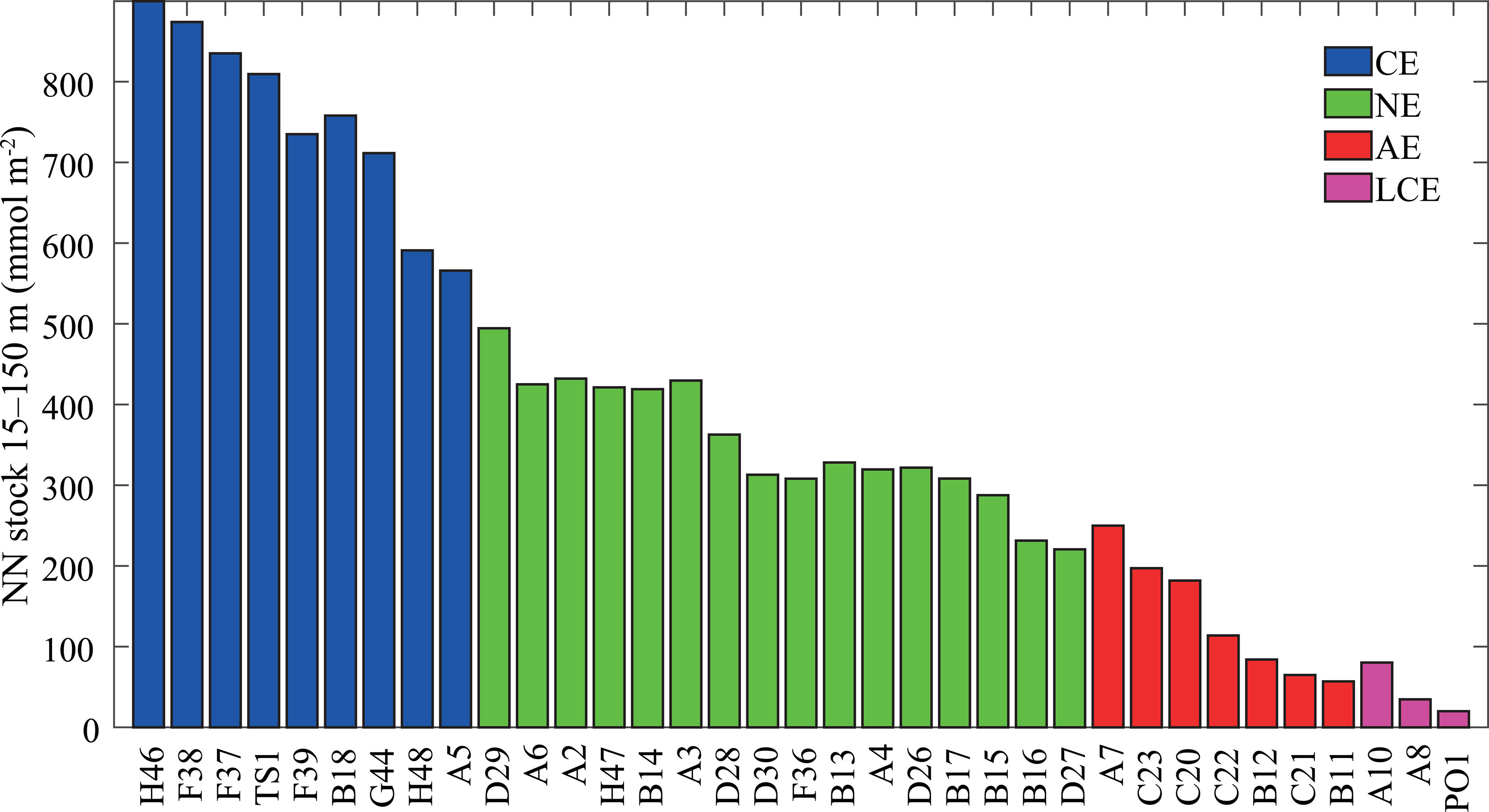
Figure 10 Depth-integrated NN from 15 to 150 m (NN_int-150, mmol m^-2) of profiles interpolated by the PCHIP method. The blue, green, red, and magenta bars correspond to the cyclonic (CE), no eddy (NE), anticyclonic (AE), and Poseidon groups, respectively. The stations were ranked based on NN_int-200 from highest (H46) to lowest (PO1) as in Figure 4.

The variability within groups is well represented with CE stations given that four cyclonic eddies that influenced nine stations were present in the sampling grid during XIXIMI-5 (Figure 1). As the CE of the Bay of Campeche influenced six stations, we were also able to explore the variability within a given eddy. For example, the difference in the NN stock at 150 m between stations H46 (located in the Bay of Campeche) and B18 (located in the LC) was 142 mmol m^-2 (Figure 10). Although altimetric and hydrographic measurements indicated that station B18 was under relatively intense cyclonic influence, its NN stock was lower than that of station H46. Differences in nutrient stocks between stations in the LC domain and stations of the interior of the gulf are likely due to the fact that respiration in the subsurface water of the LC is lower than in the water of the interior of the gulf (Figure 1E), where less oxygenated waters due to respiration are observed in the Bay of Campeche (Jochens and DiMarco, 2008; Cervantes-Díaz et al., 2022). Within the CE of the Bay of Campeche, differences as large as 310 mmol m^-2 were observed between stations H46 and H48. As indicated by the depth of the 20°C isotherm (83 m in H46 and 117 m in H48), the differences in NN stocks resulted from the differences in the locations of stations with respect to the eddy core. Similarly, with respect to the position of the eddy core, contrasting NN stocks between AE stations were observed, as was the case with Poseidon stations PO1 (Z_CT20 = 312 m) and A10 (Z_CT20 = 207 m) with a difference of ~ 60 mmol m^-2. This value is small when compared with differences in the Bay of Campeche eddy; however, the NN stock in A10 was four times the stock in PO1, which probably resulted in a difference in primary production. Finally, the difference in the average NN stock at the cores of Poseidon (27 mmol m^-2) and Olympus (69 mmol m^-2) likely reflects the increase in NN content during the journey of Olympus towards the western gulf, which took place over several months (Meunier et al., 2018; Sosa-Gutiérrez et al., 2020). Such increases likely result from isopycnal relaxation and vertical mixing (Sosa-Gutiérrez et al., 2020) in addition to the increased respiration in subsurface waters as LCEs age (Jochens and DiMarco, 2008; Cervantes-Díaz et al., 2022).

Although our campaign was not eddy-centric, the density of the sampling grid was sufficient to capture the spatial variability of water column properties due to mesoscale eddies in the deep-water region of the gulf. The NN stock in background waters is apparently well characterized with a value of ~ 350 mmol m^-2, as indicated by the low variability among stations within this group (Figure 4A). On the other hand, considering that Poseidon was the most intense LCE in the last two decades (Sosa-Gutiérrez et al., 2020) and that it was sampled when it had recently detached, the value of 20 mmol m^-2 estimated at its core is probably a reference limit for the lowest NN stock at 150 m that may be found in AEs in the GM. During XIXIMI-5, the ageing Olympus was located near the western slope and was only characterized by four stations, with a maximum of 114 mmol m^-2 (C22). This value likely depended on the location of the station with regard to the eddy core, and higher stocks may have been observed near the edges. To the best of our knowledge, Biggs and Müller-Karger (1994) published the only eddy-centric study reporting NN concentrations in both AEs and CEs in the northwestern GM from which we estimated the NN stock (see their Figures 2B, 7B). Estimates for AEs were mostly 55–200 mmol m^-2 (although a maximum of 300 mmol m^-2 was obtained) and ~ 800–1200 mmol m^-2 in the case of CEs. The higher values observed in some stations by Biggs & Müller-Karger (1994) with respect to the upper limits for AEs and CEs in our study may be due to differences in the positions of stations with respect to the eddy edge, the degree of eddy dissipation during interactions with the continental slope, and the sampling season, among others.

Primary production estimates < 100 g C m^-2 yr^-1 that are mostly based on satellite chlorophyll-a measurements indicate that the offshore waters in the GM are oligotrophic (Heileman and Rabalais, 2009; Müller-Karger et al., 2015; Damien et al., 2018). The relatively low productivity of the GM is largely determined by the limited supply of nutrients, particularly dissolved inorganic nitrogen, to the euphotic zone in this marginal sea (Gomez et al., 2018; Howe et al., 2020; Kim et al., 2020). However, the GM is less oligotrophic than the subtropical gyres of the North Atlantic and North Pacific oceans (Huston and Wolverton, 2009). This difference may be partially explained by the larger NN stock in the euphotic zone in the GM that resulted in average values in background waters of ~ 350 mmol m^-2 in our study. Based on the NN profiles reported by Bahamón and Cruzado (2003) and Cianca et al. (2007), we estimated an NN stock range of 60–170 mmol m^-2 in background waters in the North-East and North-West Atlantic Ocean and an interval of 2–100 mmol m^-2 in the North Pacific Central Gyre from the data obtained from Seki et al. (2001); Bidigare et al. (2003); Rii et al. (2008); Huang and Xu (2018). The differences in the NN stock in the upper 150 m between the gulf and the central gyres are the result of a shallower and steeper nitracline in the GM (Omand and Mahadevan, 2015). Consequently, CEs in the gulf show higher mean NN stocks (~ 750 mmol m^-2) than the CEs in the central Pacific (50–450 mmol m^-2; Seki et al., 2001; Bidigare et al., 2003; Rii et al., 2008; Huang and Xu, 2018), making them important transient bodies of water that drive relatively high primary production. While CEs play important roles in primary production in the GM, their contributions to the N budget in the euphotic zone have yet to be evaluated.

4.4 Nitracentric and Hydrographic Classification of CLIVAR Section A22 in the Caribbean Sea

The analysis of CLIVAR Section A22 in the Caribbean Sea (supplementary material, Figure S7) indicates that our classification methodology is efficient to detect stations under the influence of mesoscale eddies in areas where these structures play important roles in controlling the spatial distribution of water properties. As indicated from the analysis of the winter campaign in the GM, the results of the spring campaign in section A22 also indicate that the station classification (and thus NN profile and stock predictions) works better when comparing hydrographic data corresponding to similar stratification conditions, that is, when stratified conditions (warm seasons) are separated from winter mixing conditions (cold seasons). Clearly, if the nitracentric and hydrographic classifications are to be applied to other regions, the BFV and NN_int-z intervals must be defined based on local hydrographic conditions.

5 Conclusion

Mesoscale eddies play important roles in determining the availability of nutrients in the upper layer of the ocean and consequently influence important biogeochemical processes that operate in the euphotic zone and upper mesopelagic layer. Due to the ubiquity of these structures in the deep-water region of the GM, it is highly probable that when oceanographic surveys are conducted with regional coverage, such as the one in this study, some sampling stations will be under the influence of these structures. Although satellite altimetry is a useful tool for locating mesoscale eddies, SLA and ADT do not reflect the magnitude of the influence of mesoscale eddies on the NN stock with the same clarity as hydrographic data. The BFVs and NN_int-z were highly correlated and produced excellent classifications of the sampling stations into NE, CE, and AE groups. These classifications are more effective for studying the effects of mesoscale eddies on nutrient distributions and those of other biogeochemical and hydrographic properties than classifications based on the criteria that have been previously used in the GM, such as the depth of the 6°C isotherm.

Through third order polynomials and the BFVs, the NN stock and vertical NN profiles can be well predicted in the interval of 100–500 m. Thus, the BFVs that are obtained with CTD measurements at the time of the cast, such as the depth of the 20°C isotherm or the 26 kg m^-3 isopycnal, will allow researchers to determine if a station is under the influence of a CE or AE or if it is free of eddy influence at the time of sampling. In addition, our results permit estimates of the NN stock, which are valuable for studies of primary production and the physical and biogeochemical drivers of planktonic community dynamics in the GM, including numerical modeling studies (Biddanda and Benner, 1997; Williams et al., 2015). Additionally, the correlations presented in this study allow for NN profiles to be reconstructed from the large number of existing hydrographic profiles of the GM, such as those available in the APEX float database (Pasqueron de Fommervault et al., 2017) or the detailed hydrographic profiles that were recently obtained with gliders inside specific eddies like the LCE Poseidon (Sosa-Gutiérrez et al., 2020). These reconstructed NN profiles will improve coverage within the gulf and improve physical-biogeochemical models by providing improved definitions of regional open-boundary conditions, minimizing the use of relatively large-scale nutrient climatologies that require extending the numerical model domain and computational cost. Our results can be used to calibrate nitrate sensors mounted on BGC-Argo profiling floats for future measurements in the GM.

The nitracentric and hydrographic classification methodology developed in our study is useful for classifying stations based on the influence of mesoscale eddies and vertical NN content, and may be applied to other oligotrophic deep-water regions, such as the central region of the Caribbean Sea, where mesoscale eddies play important roles in controlling the distributions of hydrographic and biogeochemical properties.

Data Availability Statement

The discrete dataset (nitrate + nitrite) for this article is available from Camacho-Ibar, Muñóz Anderson, Ávila López, and Hakspiel Segura (2021): Water column nitrate+nitrite and phosphate from samples collected during the XIXIMI-5 oceanographic cruise in the Gulf of Mexico in June 2016. PANGAEA, https://doi.org/10.1594/PANGAEA.934036. Continuous CTD data are available upon request to the corresponding author or the Consorcio de Investigación del Golfo de México (CIGoM, sherzka@cigom.org), which owns the data.

Author Contributions

JV-A performed data analysis, developed the methodology and wrote the initial draft. VC-I acquired the funding, took part in the discussions, data analysis, and modified the manuscript. RD took part in the data analysis. RD, AT-C, JV-G, and EL-S participated to the discussions and contributed to the improvement of the manuscript. All authors contributed to the article and approved the submitted version.

Funding

This research was funded by the Mexican National Council for Science and Technology-Mexican Ministry of Energy-Hydrocarbon Fund [project number 201441]. This is a contribution of the Gulf of Mexico Research Consortium (CIGoM). We acknowledge PEMEX’s specific request to the Hydrocarbon Fund to address the environmental effects of oil spills in the Gulf of Mexico. JV-A thanks the Mexican National Council for Science and Technology (CONACyT) for the PhD scholarship [grant number 932232]. Moreover, he thanks the Mexican government and OEA for the scholarship PAEC CONACYT-OEA-AMEXCID received in 2018.

Conflict of Interest

The authors declare that the research was conducted in the absence of any commercial or financial relationships that could be construed as a potential conflict of interest.

Publisher’s Note

All claims expressed in this article are solely those of the authors and do not necessarily represent those of their affiliated organizations, or those of the publisher, the editors and the reviewers. Any product that may be evaluated in this article, or claim that may be made by its manufacturer, is not guaranteed or endorsed by the publisher.

Acknowledgments

We thank Mauricio Muñoz-Anderson and María del Carmen Ávila-López for dissolved inorganic nutrient analyses. We thank the crew and scientists of the research vessel involved in sampling and processing. MDT_CNES-CLS18 data were produced by Collecte Localisation Satellites (CLS) Space Oceanography Division and distributed by the Archiving, Validation, and Interpretation of Satellite Oceanographic Data (Aviso+), with support from the Centre National d’Etudes Spatiales (CNES; https://www.aviso.altimetry.fr/). Satellite altimeter data was provided by Ssalto/Duacs with the support of CNES and distributed by the Copernicus Marine and Environment Monitoring Service (CMEMS). The XIXIMI-5 bottle dataset for this research can be accessed at Pangaea (https://doi.org/10.1594/PANGAEA.934036). JV-A thanks the PhD program in Coastal Oceanography of the Facultad de Ciencias Marinas (FCM) and Instituto de Investigaciones Oceanológicas (IIO) of the Universidad Autónoma de Baja California (UABC). We thank the Reviewers for their positive comments and careful reviews, which helped to improve the manuscript.

Supplementary Material

The Supplementary Material for this article can be found online at: https://www.frontiersin.org/articles/10.3389/fmars.2022.827574/full#supplementary-material

References

Abdulla C. P., Alsaafani M. A., Alraddadi T. M., Albarakati A. M. (2016). Estimation of Mixed Layer Depth in the Gulf of Aden: A New Approach. PloS One 11 (10), e0165136. doi: 10.1371/journal.pone.0165136

PubMed Abstract | CrossRef Full Text | Google Scholar

Armstrong F. A. J., Stearns C. R., Strickland J. D. H. (1967). The Measurement of Upwelling and Subsequent Biological Process by Means of the Technicon Autoanalyzer® and Associated Equipment. Deep Sea Res. Oceanogr. Abstracts. 14 (3), 381–389. doi: 10.1016/0011-7471(67)90082-4

CrossRef Full Text | Google Scholar

Assassi C., Morel Y., Vandermeirsch F., Chaigneau A., Pegliasco C., Morrow R., et al. (2016). An Index to Distinguish Surface- and Subsurface-Intensified Vortices From Surface Observations. J. Phys. Oceanogr. 46 (8), 2529–2552. doi: 10.1175/JPO-D-15-0122.1

CrossRef Full Text | Google Scholar

Bahamón N., Cruzado A. (2003). Modelling Nitrogen Fluxes in Oligotrophic Environments: NW Mediterranean and NE Atlantic. Ecol. Model. 163, 223–244. doi: 10.1016/S0304-3800(03)00007-3

CrossRef Full Text | Google Scholar

Barone B., Coenen A., Beckett S. J. R., Weitz J., Karl D. (2019). The Ecological and Biogeochemical State of the North Pacific Subtropical Gyre Is Linked to Sea Surface Height. J. Mar. Res. 77, 215–245. doi: 10.1357/002224019828474241

CrossRef Full Text | Google Scholar

Benitez-Nelson C. R., McGillicuddy D. J. (2008). Mesoscale Physical–Biological–Biogeochemical Linkages in the Open Ocean: An Introduction to the Results of the E-Flux and EDDIES Programs. Deep Sea Res. Part II Top. Stud. Oceanogr. 55 (10), 1133–1138. doi: 10.1016/j.dsr2.2008.03.001

CrossRef Full Text | Google Scholar

Biddanda B., Benner R. (1997). Major Contribution From Mesopelagic Plankton to Heterotrophic Metabolism in the Upper Ocean. Deep Sea Res. Part I Oceanogr. Res. Pap. 44 (12), 2069–2085. doi: 10.1016/S0967-0637(97)00045-9

CrossRef Full Text | Google Scholar

Bidigare R. R., Benitez-Nelson C., Leonard C. L., Quay P. D., Parsons M. L., Foley D. G., et al. (2003). Influence of a Cyclonic Eddy on Microheterotroph Biomass and Carbon Export in the Lee of Hawaii. Geophys. Res. Lett. 30, 51–54. doi: 10.1029/2002GL016393

CrossRef Full Text | Google Scholar

Biggs D. C., Müller-Karger F. E. (1994). Ship and Satellite Observations of Chlorophyll Stocks in Interacting Cyclone-Anticyclone Eddy Pairs in the Western Gulf of Mexico. J. Geophys. Res. Ocean 99 (C4), 7371–7384. doi: 10.1029/93JC02153

CrossRef Full Text | Google Scholar

Brokaw R. J., Subrahmanyam B., Trott C. B., Chaigneau A. (2020). Eddy Surface Characteristics and Vertical Structure in the Gulf of Mexico From Satellite Observations and Model Simulations. J. Geophys. Res. Ocean. 125 (2), e2019JC015538. doi: 10.1029/2019JC015538

CrossRef Full Text | Google Scholar

Bunge L., Ochoa J., Badan A., Candela J., Sheinbaum J. (2002). Deep Flows in the Yucatan Channel and Their Relation to Changes in the Loop Current Extension. J. Geophys. Res. Ocean. 107 (C12), 26-1-26–27. doi: 10.1029/2001JC001256

CrossRef Full Text | Google Scholar

Cervantes-Díaz G. Y., Hernández-Ayón J. M., Zirino A., Herzka S. Z., Camacho-Ibar V., Norzagaray O., et al. (2022). Understanding Upper Water Mass Dynamics in the Gulf of Mexico by Linking Physical and Biogeochemical Features. J. Mar. Syst. 225, 103647. doi: 10.1016/j.jmarsys.2021.103647

CrossRef Full Text | Google Scholar

Chang Y.-L., Oey L.-Y. (2012). Why Does the Loop Current Tend to Shed More Eddies in Summer and Winter? Geophys. Res. Lett. 39, L050605. doi: 10.1029/2011GL050773

CrossRef Full Text | Google Scholar

Chen X., Schallenberg C., Phillips H., Chase Z. (2021). Biogeochemical Characteristics of Eddies in the East Australian Current Depend on Eddy Type, History and Location. J. Mar. Syst. 216, 103512. doi: 10.1016/j.jmarsys.2021.103512

CrossRef Full Text | Google Scholar

Cianca A., Helmke P., Mouriño B., Rueda M. J., Llinás O., Neuer S. (2007). Decadal Analysis of Hydrography and In Situ Nutrient Budgets in the Western and Eastern North Atlantic Subtropical Gyre. J. Geophys. Res. Ocean. 112 (C7), C07025. doi: 10.1029/2006JC003788

CrossRef Full Text | Google Scholar

Damien P., Pasqueron de Fommervault O., Sheinbaum J., Jouanno J., Camacho-Ibar V., Duteil O. (2018). Partitioning of the Open Waters of the Gulf of Mexico Based on the Seasonal and Interannual Variability of Chlorophyll Concentration. J. Geophys. Res. Ocean. 123 (4), 2592–2614. doi: 10.1002/2017JC013456

CrossRef Full Text | Google Scholar

Dorado S., Rooker J., Wissel B., Quigg A. (2012). Isotope Baseline Shifts in Pelagic Food Webs of the Gulf of Mexico. Mar. Ecol. Prog. Ser. 464, 37–49. doi: 10.3354/meps09854

CrossRef Full Text | Google Scholar

Dukhovskoy D. S., Leben R. R., Chassignet E. P., Hall C. A., Morey S. L., Nedbor-Gross R. (2015). Characterization of the Uncertainty of Loop Current Metrics Using a Multidecadal Numerical Simulation and Altimeter Observations. Deep Sea Res. Part I Oceanogr. Res. Pap. 100, 140–158. doi: 10.1016/j.dsr.2015.01.005

CrossRef Full Text | Google Scholar

Durán-Campos E., Salas de Leon D., Monreal-Gómez M., Coria-Monter E. (2017). Patterns of Chlorophyll-A Distribution Linked to Mesoscale Structures in Two Contrasting Areas Campeche Canyon and Bank, Southern Gulf of Mexico. J. @ Sea Res. 123, 30–38. doi: 10.1016/j.seares.2017.03.013

CrossRef Full Text | Google Scholar

Echeverri-García L., del P., Daudén-Bengoa G., Compaire J. C., Jiménez-Rosenberg S. P. A., Pérez-Brunius P., et al. (2022). Variability of Fish Larvae Assemblages Relative to Mesoscale Features in the Deep Water Region of the Southern Gulf of Mexico. Hydrobiologia 849, 1471–1493. doi: 10.1007/s10750-022-04797-w

CrossRef Full Text | Google Scholar

Elliott B. A. (1982). Anticyclonic Rings in the Gulf of Mexico. J. Phys. Oceanogr. 12 (11), 1292–1309. doi: 10.1175/1520-0485(1982)012<1292:ARITGO>2.0.CO;2

CrossRef Full Text | Google Scholar

Fritsch F. N., Carlson R. E. (1980). Monotone Piecewise Cubic Interpolation. SIAM J. Numer. Anal. 17 (2), 238–246. doi: 10.1137/0717021

CrossRef Full Text | Google Scholar

Fu L.-L., Chelton D. B., Le Traon P.-Y., Morrow R. (2010). Eddy Dynamics From Satellite Altimetry. Oceanography 23 (4), 14–25. doi: 10.5670/oceanog.2010.02

CrossRef Full Text | Google Scholar

Gaube P., Braun C. D., Lawson G. L., McGillicuddy D. J., Penna A. D., Skomal G. B., et al. (2018). Mesoscale Eddies Influence the Movements of Mature Female White Sharks in the Gulf Stream and Sargasso Sea. Sci. Rep. 8 (1), 7363. doi: 10.1038/s41598-018-25565-8

PubMed Abstract | CrossRef Full Text | Google Scholar

Gomez F. A., Lee S.-K., Liu Y., Hernandez F. J. Jr., Müller-Karger F. E., Lamkin J. T. (2018). Seasonal Patterns in Phytoplankton Biomass Across the Northern and Deep Gulf of Mexico: A Numerical Model Study. Biogeosciences 15 (11), 3561–3576. doi: 10.5194/bg-15-3561-2018

CrossRef Full Text | Google Scholar

Hamilton P., Fargion G., Biggs D. (1999). Loop Current Eddy Paths in the Western Gulf of Mexico. J. Phys. Oceanogr. 29, 1180–1207. doi: 10.1175/1520-0485(1999)029<1180:LCEPIT>2.0.CO;2

CrossRef Full Text | Google Scholar

Hamilton P., Leben R., Bower A., Furey H., Pérez-Brunius P. (2018). Hydrography of the Gulf of Mexico Using Autonomous Floats. J. Phys. Oceanogr. 48 (4), 773–794. doi: 10.1175/JPO-D-17-0205.1

CrossRef Full Text | Google Scholar

Heileman S., Rabalais N. (2009). XV-50 Gulf of Mexico: LME\# 5. The UNEP Large Marine Ecosystem Report. A Perspective on the Changing Condition in LMEs of the World’s Regional Seas Vol. 182 (Nairobi, Kenya: UNEP Regional Seas Report and Studies), 673–688.

Google Scholar

Hernández-Hernández N., Arístegui J., Montero M. F., Velasco-Senovilla E., Baltar F., Marrero-Díaz Á, et al. (2020). Drivers of Plankton Distribution Across Mesoscale Eddies at Submesoscale Range. Front. Mar. Sci. 7, 667. doi: 10.3389/fmars.2020.00667

CrossRef Full Text | Google Scholar

Hernández-Sánchez O. G., Camacho-Ibar V. F., Fernández Álamo M. A., Herzka S. Z. (2022). Nitrogen Sources (NO3– vs N2 Fixation) Inferred From Bulk δ15n Values of Zooplankton From the Deep Water Region of the Gulf of Mexico. J. Plankton Res. 44 (1), 48–67. doi: 10.1093/plankt/fbab089

CrossRef Full Text | Google Scholar

Howe S., Miranda C., Hayes C. T., Letscher R. T., Knapp A. N. (2020). The Dual Isotopic Composition of Nitrate in the Gulf of Mexico and Florida Straits. J. Geophys. Res. Oceans. 125 (9), e2020JC016047. doi: 10.1029/2020JC016047

CrossRef Full Text | Google Scholar

Hsu A. C., Boustany A. M., Roberts J. J., Chang J.-H., Halpin P. N. (2015). Tuna and Swordfish Catch in the U.S. Northwest Atlantic Longline Fishery in Relation To Mesoscale Eddies. Fish. Oceanogr. 24 (6), 508–520. doi: 10.1111/fog.12125

PubMed Abstract | CrossRef Full Text | Google Scholar

Huang P.-Q., Lu Y.-Z., Zhou S.-Q. (2018). An Objective Method for Determining Ocean Mixed Layer Depth With Applications to WOCE Data. J. Atmos. Ocean. Technol. 35 (3), 441–458. doi: 10.1175/JTECH-D-17-0104.1

CrossRef Full Text | Google Scholar

Huang J., Xu F. (2018). Observational Evidence of Subsurface Chlorophyll Response to Mesoscale Eddies in the North Pacific. Geophys. Res. Lett. 45 (16), 8462–8470. doi: 10.1029/2018GL078408

CrossRef Full Text | Google Scholar

Huston M. A., Wolverton S. (2009). The Global Distribution of Net Primary Production: Resolving the Paradox. Ecol. Monogr. 79 (3), 343–377. doi: 10.1890/08-0588.1

CrossRef Full Text | Google Scholar

Hydes D. J., Aoyama M., Aminot A., Bakker K., Becker S., Coverly S., et al. (2010). Determination of Dissolved Nutrients (N, P, Si) in Seawater With High Precision and Inter-Comparability Using Gas-Segmented Continuous Flow Analysers. Go-sh. Repeat Hydrogr. Man. A Collect. Expert Reports Guidel. IOCCP Rep. No 14, ICPO Publ. Ser. No. 134, version 1, 2010.

Google Scholar

Jochens A. E., DiMarco S. F. (2008). Physical Oceanographic Conditions in the Deepwater Gulf of Mexico in Summer 2000–2002. Deep Sea Res. Part II Top. Stud. Oceanogr. 55 (24), 2541–2554. doi: 10.1016/j.dsr2.2008.07.003

CrossRef Full Text | Google Scholar

Jolliff J. K., Kindle J. C., Penta B., Helber R., Lee Z., Shulman I., et al. (2008). On the Relationship Between Satellite-Estimated Bio-Optical and Thermal Properties in the Gulf of Mexico. J. Geophys. Res. Biogeosci. 113, G01024. doi: 10.1029/2006JG000373

CrossRef Full Text | Google Scholar

Kim J., Chapman P., Rowe G., DiMarco S. F., Thornton D. C. O. (2020). Implications of Different Nitrogen Input Sources for Potential Production and Carbon Flux Estimates in the Coastal Gulf of Mexico (GOM) and Korean Peninsula Coastal Waters. Ocean Sci. 16 (1), 45–63. doi: 10.5194/os-16-45-2020

CrossRef Full Text | Google Scholar

Lee-Sánchez E., Camacho-Ibar V. F., Velásquez-Aristizábal J. A., Valencia-Gasti J. A., Samperio-Ramos G. (2022). Impacts of Mesoscale Eddies on the Nitrate Distribution in the Deep-Water Region of the Gulf of Mexico. J. Mar. Syst. 229, 103721. doi: 10.1016/j.jmarsys.2022.103721

CrossRef Full Text | Google Scholar

Linacre L., Durazo R., Camacho-Ibar V. F., Selph K. E., Lara-Lara J. R., Mirabal-Gómez U., et al. (2019). Picoplankton Carbon Biomass Assessments and Distribution of Prochlorococcus Ecotypes Linked to Loop Current Eddies During Summer in the Southern Gulf of Mexico. J. Geophys. Res. Ocean. 124 (11), 8342–8359. doi: 10.1029/2019JC015103

CrossRef Full Text | Google Scholar

Linacre L., Lara-Lara R., Camacho-Ibar V., Herguera J. C., Bazán-Guzmán C., Ferreira-Bartrina V. (2015). Distribution Pattern of Picoplankton Carbon Biomass Linked to Mesoscale Dynamics in the Southern Gulf of Mexico During Winter Conditions. Deep Sea Res. Part I Oceanogr. Res. Pap. 106, 55–67. doi: 10.1016/j.dsr.2015.09.009

CrossRef Full Text | Google Scholar

McGillicuddy D. J. (2015). Formation of Intrathermocline Lenses by Eddy–Wind Interaction. J. Phys. Oceanogr. 45 (2), 606–612. doi: 10.1175/JPO-D-14-0221.1

CrossRef Full Text | Google Scholar

McGillicuddy D. J. (2016). Mechanisms of Physical-Biological-Biogeochemical Interaction at the Oceanic Mesoscale. Annu. Rev. Marine Sci. 8 (1), 125–159. doi: 10.1146/annurev-marine-010814-015606

CrossRef Full Text | Google Scholar

McGillicuddy D. J., Robinson A. R. (1997). Eddy-Induced Nutrient Supply and New Production in the Sargasso Sea. Deep Sea Res. Part I Oceanogr. Res. Pap. 44 (8), 1427–1450. doi: 10.1016/S0967-0637(97)00024-1

CrossRef Full Text | Google Scholar

McGillicuddy D. J., Robinson A. R., Siegel D. A., Jannasch H. W., Johnson R., Dickey, et al. (1998). Influence of Mesoscale Eddies on New Production in the Sargasso Sea. Nature 394 (6690), 263–266. doi: 10.1038/28367

CrossRef Full Text | Google Scholar

Meunier T., Pallás-Sanz E., Tenreiro M., Portela E., Ochoa J., Ruiz-Angulo A., et al. (2018). The Vertical Structure of a Loop Current Eddy. J. Geophys. Res. Ocean. 123 (9), 6070–6090. doi: 10.1029/2018JC013801

CrossRef Full Text | Google Scholar

Müller-Karger F., Smith J., Werner S., Chen R., Roffer M., Liu Y., et al. (2015). Natural Variability of Surface Oceanographic Conditions in the Offshore Gulf of Mexico. Prog. Oceanogr. 134, 54–76. doi: 10.1016/j.pocean.2014.12.007

CrossRef Full Text | Google Scholar

Omand M. M., Mahadevan A. (2015). The Shape of the Oceanic Nitracline. Biogeosciences 12 (11), 3273–3287. doi: 10.5194/bg-12-3273-2015

CrossRef Full Text | Google Scholar

Oschlies A., Garçon V. (1998). Eddy-Induced Enhancement of Primary Production in a Model of the North Atlantic Ocean. Nature 394(6690), 266–269. doi: 10.1038/28373

CrossRef Full Text | Google Scholar

Pasqueron de Fommervault O., Perez-Brunius P., Damien P., Camacho-Ibar V., Sheinbaum J. (2017). Temporal Variability of Chlorophyll Distribution in the Gulf of Mexico: Bio-Optical Data From Profiling Floats. Biogeosciences 14 (24), 5647–5662. doi: 10.5194/bg-14-5647-2017

CrossRef Full Text | Google Scholar

Pérez-Brunius P., García-Carrillo P., Dubranna J., Sheinbaum J., Candela J. (2013). Direct Observations of the Upper Layer Circulation in the Southern Gulf of Mexico. Deep Sea Res. Part II Top. Stud. Oceanogr. 85, 182–194. doi: 10.1016/j.dsr2.2012.07.020

CrossRef Full Text | Google Scholar

Portela E., Tenreiro M., Pallàs-Sanz E., Meunier T., Ruiz-Angulo A., Sosa-Gutiérrez R., et al. (2018). Hydrography of the Central and Western Gulf of Mexico. J. Geophys. Res. Ocean. 123 (8), 5134–5149. doi: 10.1029/2018JC013813

CrossRef Full Text | Google Scholar

Rii Y. M., Brown S. L., Nencioli F., Kuwahara V., Dickey T., Karl D. M., et al. (2008). The Transient Oasis: Nutrient-Phytoplankton Dynamics and Particle Export in Hawaiian Lee Cyclones. Deep Sea Res. Part II Top. Stud. Oceanogr. 55 (10), 1275–1290. doi: 10.1016/j.dsr2.2008.01.013

CrossRef Full Text | Google Scholar

Rudnick D. L., Gopalakrishnan G., Cornuelle B. D. (2015). Cyclonic Eddies in the Gulf of Mexico: Observations by Underwater Gliders and Simulations by Numerical Model. J. Phys. Oceanogr. 45 (1), 313–326. doi: 10.1175/JPO-D-14-0138.1

CrossRef Full Text | Google Scholar

Salmerón-García O., Zavala-Hidalgo J., Mateos-Jasso A., Romero-Centeno R. (2011). Regionalization of the Gulf of Mexico From Space-Time Chlorophyll-A Concentration Variability. Ocean Dyn. 61 (4), 439–448. doi: 10.1007/s10236-010-0368-1

CrossRef Full Text | Google Scholar

Sarma V. V. S. S., Jagadeesan L., Dalabehera H. B., Rao D. N., Kumar G. S., Durgadevi D. S., et al. (2018). Role of Eddies on Intensity of Oxygen Minimum Zone in the Bay of Bengal. Cont. Shelf Res. 168, 48–53. doi: 10.1016/j.csr.2018.09.008

CrossRef Full Text | Google Scholar

Schmitz W. J. Jr. (2005). “Cyclones and Westward Propagation in the Shedding of Anticyclonic Rings From the Loop Current. Washingt. DC Am. Geophys. Union Geophys. Monogr. Ser. 161, 241–261. doi: 10.1029/161GM18

CrossRef Full Text | Google Scholar

Seki M. P., Polovina J. J., Brainard R. E., Bidigare R. R., Leonard C. L., Foley D. G. (2001). Biological Enhancement at Cyclonic Eddies Tracked With GOES Thermal Imagery in Hawaiian Waters. Geophys. Res. Lett. 28 (8), 1583–1586. doi: 10.1029/2000GL012439

CrossRef Full Text | Google Scholar

Shropshire T. A., Morey S. L., Chassignet E. P., Bozec A., Coles V. J., Landry M. R., et al. (2020). Quantifying Spatiotemporal Variability in Zooplankton Dynamics in the Gulf of Mexico With a Physical–Biogeochemical Model. Biogeosciences 17 (13), 3385–3407. doi: 10.5194/bg-17-3385-2020

CrossRef Full Text | Google Scholar

Sosa-Gutiérrez R., Pallàs-Sanz E., Jouanno J., Chaigneau A., Candela J., Tenreiro M. (2020). Erosion of the Subsurface Salinity Maximum of the Loop Current Eddies From Glider Observations and a Numerical Model. J. Geophys. Res. Ocean. 125, e2019JC015397. doi: 10.1029/2019JC015397

CrossRef Full Text | Google Scholar

Williams A. K., McInnes A. S., Rooker J. R., Quigg A. (2015). Changes in Microbial Plankton Assemblages Induced by Mesoscale Oceanographic Features in the Northern Gulf of Mexico. PloS One 10 (9), e0138230. doi: 10.1371/journal.pone.0138230

PubMed Abstract | CrossRef Full Text | Google Scholar

Zavala-Hidalgo J., Morey S. L., O’Brien J. J., Zamudio L. (2006). On the Loop Current Eddy Shedding Variability. Atmosfera 19, 41–48.

Google Scholar