Dynamic Habitat Models Reflect Interannual Movement of Cetaceans Within the California Current Ecosystem

1 Introduction

The management of transboundary marine species, such as cetaceans whose distributions span waters of two or more nations, is challenging because laws for managing anthropogenic impacts vary among nations, and data may only be available for a portion of each species’ range. Survey effort is often restricted to waters of a single country due to funding constraints and nationally-driven management objectives. However, there has been increasing recognition that successful monitoring and conservation of highly-mobile cetaceans require coordinated surveys across broader areas to capture changes in species distribution and abundance as ocean conditions vary. The International Whaling Commission’s SOWER (Southern Ocean Whale and Ecosystem Research) and POWER (Pacific Ocean Whale and Ecosystem Research) programs have conducted large-scale surveys of the Southern Ocean and North Pacific Ocean, respectively, since the 1990s to assess and monitor whale populations (see e.g., Sekiguchi et al., 2010; Matsuoka et al., 2021). In the Atlantic Ocean, a series of multinational cetacean surveys (SCANS, T-NASS) have assessed cetacean abundance and distribution in a coordinated manner within the northeast Atlantic (Hammond et al., 2002; Hammond et al., 2013; Hammond et al., 2021) and across the far northern Atlantic between Norway and Canada (see Desportes et al., 2019). These comprehensive efforts have allowed management considerations at biologically and ecologically relevant scales and within a multi-national framework.

Along the Pacific Coast of North America, cetacean surveys conducted by the National Oceanic and Atmospheric Administration (NOAA) since 1991 have primarily focused on U.S. waters of the California Current Ecosystem (CCE) (e.g., Barlow, 1995; Barlow and Forney, 2007; Barlow, 2016). However, the CCE is a highly dynamic marine environment, and the distributions of many cetacean species extend into Canadian, Mexican and/or international waters. Abundance estimates for some species have been highly variable off the U.S. West Coast (Barlow and Forney, 2007; Barlow, 2016), e.g., estimates of striped dolphin (Stenella coeruleoalba) abundance ranged from a low of 8,614 animals (CV = 0.51) in 1996 to a high of 90,433 animals (CV = 0.24) in 2014 (Barlow, 2016), reflecting range shifts rather than true population changes. Similar distribution shifts have created management issues for other warm-temperate species such as short-beaked and long-beaked common dolphins (Delphinus delphis delphis and D. d. bairdii), whose numbers tend to increase in U.S. waters during warm water conditions (Barlow, 2016; Becker et al., 2018; Becker et al., 2020a). Recognizing the need to cover a broader geographic range, the most recent (2018) NOAA cetacean assessment survey covered waters from Vancouver Island, Canada to Baja California, México (Henry et al., 2020).

Habitat-based models, or species distribution models (SDMs), are powerful tools for documenting shifts in cetacean distribution due to changing environmental conditions (Becker et al., 2018; Boyd et al., 2018). SDMs estimate density as a continuous function of habitat variables (e.g., sea surface temperature, seafloor depth) and thus, within the study area that was modeled, densities can be predicted at all locations where these habitat variables can be measured or estimated. Spatial habitat models therefore allow estimates of cetacean densities on finer scales than traditional line-transect or mark-recapture analyses. Abundance estimates (for a study area) derived from habitat-based models also tend to be more stable from one year to the next, in part because the models that generate the annual estimates are built from data collected across multiple years, whereas abundance estimates from design-based methods rely strictly on encounter rate data for an individual year and are thus subject to increased sampling variance (Barlow et al., 2009; Forney et al., 2012; Becker et al., 2020b);. For those species that exhibit substantial interannual distribution shifts in and out of U.S. waters, SDMs that incorporate survey data that better sample the broader geographic distribution range of these species, and include a wider environmental covariate space, should provide greater insight into observed abundance changes.

SDMs have been developed for cetaceans within U.S. West Coast waters from systematic ship survey data collected by NOAA’s Southwest Fisheries Science Center (SWFSC) since 1991 (Forney, 2000; Barlow et al., 2009; Becker et al., 2010; Forney et al., 2012; Becker et al., 2014; Becker et al., 2016; Becker et al., 2018; Becker et al., 2020a; Becker et al., 2020b), and multi-year average density predictions from these models have been used by the U.S. Navy to assess potential impacts on cetaceans from training and testing activities in Southern California waters as required by U.S. regulations such as the Marine Mammal Protection Act and Endangered Species Act (U.S. Department of the Navy, 2013; U.S. Department of the Navy, 2015; U.S. Department of the Navy, 2018). In addition to training and testing areas located off California, the Navy’s Southern California Range Complex extends more than 600 nmi southwest into the Pacific Ocean, encompassing waters west of the Baja California peninsula, México (U.S. Department of the Navy, 2013; U.S. Department of the Navy, 2018). Until recently, systematic survey data collected in these waters have been limited largely to transits from San Diego, California, to SWFSC study areas in the Eastern Tropical Pacific (Hamilton et al., 2009). Data from surveys conducted between 1986 and 1996 have been used to develop stratified design-based density estimates for cetaceans in the eastern Pacific at very coarse spatial resolution (i.e., 5° X 5° cells; Ferguson & Barlow, 2003), and the U.S. Navy has used these estimates to estimate potential impacts to cetaceans from their activities that occur in waters west of the Baja California peninsula (U.S. Department of the Navy, 2013; U.S. Department of the Navy, 2018). To better evaluate the potential impacts of their activities requires estimates of cetacean distribution and abundance at finer spatial scales than currently available, ideally from an SDM that is built with dynamic environmental covariates that can account for changes in oceanic conditions. It is well established that there can be dramatic shifts of many cetacean species in this region in response to changes in oceanic conditions (e.g., Forney, 2000; Barlow et al., 2009; Becker et al., 2014; Becker et al., 2017; Hazen et al., 2017; Becker et al., 2018; Abrahms et al., 2019; Becker et al., 2020a), thus underpinning the need for effective SDMs that incorporate dynamic habitat covariates.

An SDM has been developed to estimate the density of long-beaked common dolphin in waters west of the Baja California peninsula, based on SWFSC ship survey data collected between 1986 and 2006 (Gerrodette and Eguchi, 2011). The known range of long-beaked common dolphin extends from central California south into Mexican waters (Carretta et al., 2011), and yearly design-based abundance estimates for U.S. waters are highly variable for this species (Barlow, 2016). The hierarchical Bayesian model developed by Gerrodette and Eguchi (2011) estimated long-beaked common dolphin density as a function of depth, and captured this species primarily coastal distribution, but dynamic habitat variables are required to predict shifts in distribution due to environmental variability, since common dolphins exhibit shifts at seasonal and interannual time scales (Dohl et al., 1986; Heyning and Perrin, 1994; Forney and Barlow, 1998; Becker et al., 2014; Becker et al., 2020a; Becker et al., 2020b). Hierarchical Bayesian models have also been developed to estimate blue whale (Balaenoptera musculus) and short-beaked common dolphin density in the northeast Pacific Ocean as functions of absolute dynamic topography (Pardo et al., 2015). Model predictions included waters both off the U.S. and west of the Baja California peninsula but at very coarse spatial resolution (1/3°-degree cells), thus limiting their use for finer scale management applications.

In addition to the systematic survey data available from SWFSC transits through the area between 1986 and 2006, three SWFSC surveys included focused effort in waters west of the Baja California peninsula during 1993, 2009, and 2018. The 1993 survey covered the range of short-beaked common dolphins off California and Baja California (Mangels and Gerrodette, 1994) as part of a 2-year study of this species. The 2009 survey was specifically designed to sample the known range of long-beaked common dolphins along the central and southern California coast, as well as the coastal waters west of the Baja California peninsula (Carretta et al., 2011). The 2018 survey covered waters along the west coasts of southern Canada (Vancouver Island), the U.S., and waters west of the Baja California peninsula (Henry et al., 2020). Sightings from these surveys provided sufficient sample sizes to develop SDMs for many cetacean species occurring in the Southern California Current study area.

The objective of this study was to develop dynamic cetacean SDMs for as many species as possible, both to generate multi-year average density surfaces for all Southern California Current stakeholders to use in their long-term (2–7 year) environmental planning efforts, and to improve our understanding of species distribution patterns by including a broader distribution range of many species, particularly those suspected to exhibit distribution shifts between U.S. and Mexican waters (e.g., striped, and long- and short-beaked common dolphins; Dohl et al., 1986; Heyning and Perrin, 1994; Forney and Barlow, 1998; Barlow, 2016; Becker et al., 2018). Models were built for ten species with sufficient sample sizes: long-beaked common dolphin, short-beaked common dolphin, Risso’s dolphin (Grampus griseus), Pacific white-sided dolphin (Lagenorhynchus obliquidens), striped dolphin, common bottlenose dolphin (Tursiops truncatus), sperm whale (Physeter macrocephalus), blue whale, fin whale (Balaenoptera physalus), and humpback whale (Megaptera novaeangliae).

2 Materials and Methods

2.1 Study Area

For the purposes of this analysis, the study area was defined to include the area from Point Conception south to 23°N, and from the coast out to 132.5°E longitude. This region encompasses the Southern California Current System, a distinct oceanographic province that provides an ecologically meaningful study area for cetaceans (Checkley and Barth, 2009). The region west of the Baja California peninsula marks the southern limit of the California Current, a well-known eastern boundary upwelling system (Hickey, 1979). Although there are some regional differences, there is generally a continuous equatorward flow along shore near the surface (0-300m deep), and a subsurface inshore poleward flow along the Baja California peninsula and southern California coast north to Point Conception at 34.5°N latitude (Lynn and Simpson, 1987; Durazo, 2015). Although the “Inshore Countercurrent” at times is continuous around Point Conception, this headland is a well-known biogeographic boundary, marking the range limits of many marine species (Valentine, 1973; Briggs, 1974; Newman, 1979; Doyle, 1985). SWFSC survey data collected in this “Southern California Current study area” from 1992–2018 were used to create the modeling dataset, and when combined across years, provided reasonable coverage of the study area, particularly in nearshore waters where oceanic conditions are more dynamic (Figure 1). Data from SWFSC surveys that transited waters west of the Baja California peninsula prior to 1992 were not used because dynamic ocean modeled data used to develop the SDMs were not available for these earlier years.

FIGURE 1

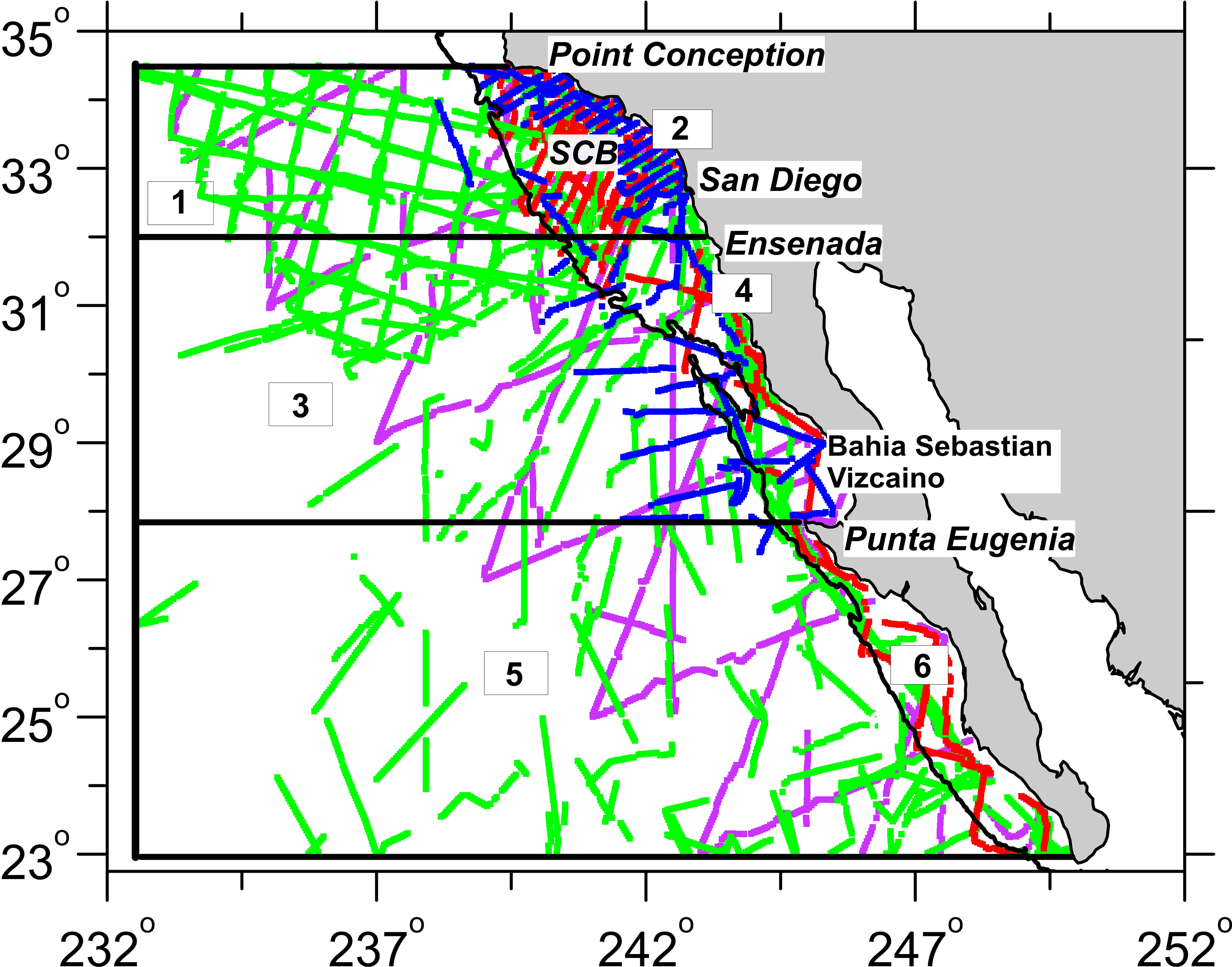
Figure 1 Completed transects for the Southwest Fisheries Science Center systematic ship surveys conducted between 1992 and 2018 in the Southern California Current study area. The colored lines show on-effort transect coverage in Beaufort sea states ≤5: purple lines = 1993 survey, blue lines = 2009 survey, red lines = 2018 survey, green lines = transits in waters west of the Baja California peninsula and surveys that included U.S. waters within the Southern California Bight (SCB). Also shown are the six geographic strata used to evaluate the accuracy of the spatial patterns of predicted density, with the offshore/inshore division set at the 2,000 m isobath: (1) offshore north of the approximate location of the Ensenada Front in August (EF; 32°N), (2) inshore north of the EF, (3) offshore north of Punta Eugenia, (4) inshore north of Punta Eugenia, (5) offshore south of Punta Eugenia, and (6) inshore south of Punta Eugenia.

Six geographic strata were created within the study area to assess the SDMs ability to predict spatial distribution patterns. Latitudinal boundaries were set at Punta Eugenia (28°N), which represents a faunal transition zone for several fish species (Hewitt, 1981), and the Ensenada Front, a persistent feature that separates eutrophic waters to the north from oligotrophic waters to the south (Santamaria-del-Angel et al., 2002). The Ensenada Front shifts latitudinally during the year, but 32°N was selected to divide the strata as it marks the approximate boundary of the front in August, the month with maximum survey coverage. In addition, an offshore-onshore division was made at the 2,000m isobath, which roughly represents the transition from the continental shelf to the continental rise (Figure 1).

2.2 Survey Data

Cetacean sighting data used to build the SDMs were collected in the Southern California Current study area during the summer and fall (June through early December) from 1992–2018 (Table 1) using systematic line-transect methods (Buckland et al., 2001). Surveys conducted in 1993, 1996, 2001, 2005, 2008, and 2014 covered waters from the coast to approximately 556 km offshore (Barlow and Forney, 2007; Barlow, 2016), providing comprehensive sampling of the Southern California Bight (SCB; Figure 1). The 1993, 2009 and 2018 surveys included focused efforts in coastal waters of both southern California and the Baja California peninsula (Mangels & Gerrodette, 1994; Carretta et al., 2011; Henry et al., 2020). The purpose of the remaining surveys was to sample the eastern tropical Pacific, but included systematic effort during transits within the Southern California Current study area, thus providing additional data to use in this analysis.

TABLE 1

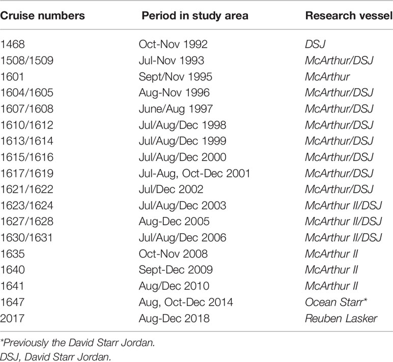
Table 1 Cetacean and ecosystem assessment surveys conducted within the Southern California Current study area during 1992–2018.

Only on-effort data collected in Beaufort sea state conditions ≤5 were used in model development. Sighting rates in sea state 5 are generally lower than in calmer sea states, but extensive past surveys by the SWFSC that included effort for sea states 0-5 have allowed for the estimation of sea-state specific correction factors (Barlow et al., 2011; Barlow, 2015). This is particularly important given that offshore areas tend to have higher sea states and excluding those segments could bias the overall models. As described below in the modeling framework subsection, the sea-state specific correction factors have been included in our models using the methods described in Becker et al. (2016).

The survey protocols were largely the same for all years (see Barlow and Forney, 2007; Henry et al., 2020) and are briefly summarized here. A team of 6 experienced visual observers were present on each survey, rotating among three observer stations every two hours. Observers at port and starboard stations searched for cetaceans between 0 and 90 degrees from the ship’s bow using 25 × 150 mounted binoculars, and a center-stationed third observer searched by eye or with handheld 7 × 50 binoculars. When cetaceans were detected within 3 nmi (5.6 km) of the trackline, the sighting was recorded at the time of the initial observation, along with distance and direction from the vessel, from which perpendicular sighting distance was calculated. Typically, the ship would then be diverted from the transect line (“closing mode”) and observers went “off-effort” to approach the animals and enable more accurate estimation of group size and species identification. All observers recorded confidential estimates of best, high, and low group size, and if the sighting included more than one species, the observers also estimated the proportional makeup of species in the group. Following identification and enumeration, the vessel angled back to the original transect line to avoid getting drawn into high-density regions (Barlow, 1997). To obtain a single group size estimate for each sighting, the best estimate from each observer was averaged (i.e., arithmetic mean), and prorated by species for multi-species groups. In addition to the sighting data, information on detection parameters (e.g., Beaufort sea state, visibility, swell height) was recorded on a laptop computer connected to the ship’s navigation system.

Systematic survey effort was conducted along predetermined tracklines at a target survey speed of 18.5 km/hr. During transits to or from port (e.g., on those surveys headed to or from the eastern tropical Pacific), transits between tracklines, or deviations from pre-determined tracklines for other purposes, the visual observers generally maintained standard data collection protocols. Although such non-systematic effort would introduce a bias when estimating encounter rates for design-based abundance estimates, heterogeneity is less of a problem for SDMs because the uneven distribution of effort can be accounted for within this statistical framework (Hedley and Buckland, 2004) while increasing sample sizes for model development. For this study we developed models for all species with >40 sightings, recognizing that ideally sample sizes would be closer to 100, but that smaller sample sizes can be used to parameterize SDMs for species that inhabit less dynamic environments, such as the offshore regions of the study area (Becker et al., 2010).

2.3 Habitat Covariates

Continuous portions of survey effort were divided into approximate 5-km segments to create samples for modelling using the approach described by Becker et al. (2010). The segment size was specifically selected based on the oceanographic processes and bathymetry of the study area so that habitat is expected to vary little within the segments. Species-specific sighting data were assigned to each segment (total number of sightings and arithmetic average group size), and habitat covariates were derived based on the segment’s geographical midpoint. Consistent with standard distance sampling methods, sighting data were truncated at 5.5 km perpendicular to the trackline to eliminate the most distant groups (Buckland et al., 2001; Miller et al., 2019) and maintain consistency with the species-specific effective-strip-width estimates derived for this study based on methods described in Barlow et al. (2011) and used to estimate cetacean densities.

Outputs from the Hybrid Coordinate Ocean Model (HYCOM; Chassignet et al., 2007) were used as dynamic predictor variables in the habitat models. HYCOM products include a global reanalysis that assimilates multiple sources of data in product development (including satellite and in situ), and outputs from HYCOM have been widely used and widely tested (https://www.hycom.org/). Daily averages for each variable served at the 0.08 degree (approximately 9 km) horizontal resolution of the HYCOM output were used in the models. The suite of potential dynamic predictors included sea surface temperature (SST) and its standard deviation [sd(SST)], calculated for a 3 × 3-pixel box around the modeling segment centroid), mixed layer depth (MLD, defined by a 0.5˚C deviation from the SST), sea surface height (SSH), sd(SSH), salinity (SAL), and sd(SAL). Contemporaneous covariates were used because they are better able to capture the interannual variations in cetacean distribution patterns within the highly dynamic California Current study area (Mannocci et al., 2017). Water depth (m) was also included as a potential predictor, derived from the ETOPO1 1-arc-min global relief model (Amante and Eakins, 2009).

The dynamic predictors were selected because they have proven effective in similar habitat models in the study area (Becker et al., 2010; Pardo et al., 2015; Becker et al., 2016; Becker et al., 2017; Becker et al., 2018; Becker et al., 2020a; Becker et al., 2020b) and they provide useful indicators for oceanographic processes that serve to increase biological production and aggregate prey. For example, SST, MLD, and SAL identify variations in upwelling and water column stratification; upwelled waters are generally colder and have higher salinity concentrations than adjacent surface waters. SSH reflects circulation and density structure since the higher density of upwelled waters in the surface layer generally results in lower sea surface heights (Talley et al., 2011), and sd(SSH) reflects the mesoscale variability of SSH. The sd(SST) variable was included to serve as a proxy for frontal regions since dynamic ocean processes such as upwelling, fronts, and eddies often result in surface SST gradients between colder upwelled water and warmer surface water.

2.4 Habitat Models

Modeling methods followed those described in Becker et al. (2020b), and are repeated here for completeness.

2.4.1 Correction Factors

During the 2018 survey, operational requirements necessitated that some of the effort be conducted in passing mode (i.e., when a cetacean/cetacean group is sighted the ship continues on course and is not diverted to the vicinity of the sighting for species identification or group size enumeration). This led to a large proportion of recorded “unidentified large whale” and “Delphinus spp.” sightings when observers could not confirm which species of large whale or common dolphin subspecies was present, respectively. Omitting these sightings from the modeling dataset would have resulted in an underestimation of animal density for blue, fin, and humpback whales, as well as both long- and short-beaked common dolphins during 2018 compared to prior years. To reduce this potential downward bias, species-specific correction factors were applied to account for unidentified animals, using the methods described in Becker et al. (2017) and summarized below.

For both the large whale and common dolphin groups, the correction factor c was estimated from the 2018 sighting data according to the simplified formula:

$\begin{array}{ll}\text{c}=1+ \frac{{\text{t}}_{unid} }{t_{tgt}+ t_{oth}}& (1)\end{array}$

where t_tgt is the number of individuals identified as the target species, t_oth is the number of individuals identified as other species within the broader species group, and t_unid is the number of unidentified individuals in that species group. Due to the potential effect of Beaufort sea state on detectability (Barlow et al., 2001; Barlow et al., 2011; Barlow, 2015), the correction factors were evaluated to determine if they varied by sea state. If so, separate correction factors were developed by sea state; otherwise a single correction factor was applied. The correction factors were applied to the numbers of animals estimated per segment in the SDMs for the common dolphin and large whale species (see equation 2 below).

The protocol for estimating sperm whale group size on SWFSC surveys has changed over the course of the 1992–2018 survey period, with less effort spent estimating group size during surveys conducted in the 1990’s. Group size estimates for larger sperm whale groups (> 2 animals) are now known to have been underestimated in the earlier surveys, and a correction factor has been estimated to account for this bias (Moore and Barlow, 2014). Prior to modeling, this correction factor (2.3x) was applied to the average group size estimates for observed sperm whale group sizes > 2 for the 1992–1999 surveys.

2.4.2 Modeling Framework

Generalized Additive Models (GAMs; Wood, 2017) were developed in R (v. 3.4.1; R Core Team, 2017) using the package “mgcv” (v. 1.8-31; Wood, 2011). One of two modeling frameworks was used for each species, depending on its group size characteristics.

For most species, GAMs were fitted using the number of individuals of the given species per transect segment (n_j, where j indexes the segments) as the response variable, which was assumed to follow a Tweedie distribution with a log link. Environmental covariates measured at each segment (x_kj, where k indexes the covariates) were included as smooth functions (f_k). Following the methods of Becker et al. (2016), effort was accounted for by using a single offset term that was the product of the area covered (A_j), the probability of detection $(\widehat{p_j})$, and the correction for detectability on the trackline $((\widehat{g{(0)}_j})$. A_jwas calculated as the product of the segment length, the truncation distance, and the number of sides surveyed, which was an issue during 2018 because coastal fog at times limited search effort to one side of the vessel. The probability of detection $(\widehat{p_j})$ was derived from species-specific detection functions based on methods of Barlow et al. (2011). The correction for detectability on the trackline $(\widehat{g{(0)}_j})$ was estimated using the method of Barlow (2015), which assumes that $\widehat{g{(0)}_j}=1$ when average Beaufort sea state on the segment was 0, and estimates g(0)_j for other sea states based on relative densities. The overall “count” models take the following form:

$\begin{array}{ll}E(n_j)=A_j\widehat{p_j}\widehat{g{(0)}_j}exp\left\{{\beta }_0+\sum _{k=1}^K{f}_k(x_{kj})\right\}\text{ where }{n}_j\sim \text{Tweedie}\left(\varphi \text{,q}\right).& (2)\end{array}$

In this equation β₀ is a model intercept and Tweedie parameters ϕ (scale) and q (power) are estimated during model fitting and dictate the mean-variance relationship of the distribution such that Var(X)=ϕE(X)^q.

For the two Delphinus species that have very large and variable group sizes (e.g., 1 to 2,000 animals per sighting), separate encounter rate and group size models were developed. Encounter rate models were built using all transect segments, regardless of whether they included sightings, using the number of sightings per segment as the response variable and a Tweedie distribution to account for overdispersion (Miller et al., 2013). Group size models were built using only those segments that included sightings, using the natural log of group size as the response variable, and a Gaussian response distribution (effectively assuming group size was log-normally distributed). To account for observed geographical differences in the size of delphinid groups (Ferguson et al., 2006; Cañadas and Hammond, 2008; Barlow, 2015) and success in previous models (Becker et al., 2018), a tensor product smooth of latitude and longitude (Wood, 2003) was the only predictor variable included in the Delphinus group size models. The group size models were therefore of the following form:

$\begin{array}{ll}E\left(lo{g}_e{s}_i\right)={\text{β}}_0+{\text{f(x}}_{\text{i}},{\text{y}}_{\mathrm{i}}\text{) where }{s}_i\sim \text{Normal.}& (3)\end{array}$

This model uses only the data where groups of animals were observed (indexed by i), where s_i is the size of the ith group, β₀ is a model intercept and f(x_i, y_i) denotes a tensor product smooth of space, evaluated at the segment location where the ith sighting was observed. The encounter rate model was fitted to all data but using the number of groups in segment j, m_j, as the response:

$\begin{array}{ll}E(m_j)=A_j\widehat{p_j}\widehat{g{\left(0\right)}_j}exp\left\{{\text{β}}_0+\sum _{k=1}^K{f}_k(x_{kj})\right\}\text{where }{m}_j\sim \text{Tweedie}(\varphi ,\text{q}).& (4)\end{array}$

Notation follows (2) above. The product of the number of groups and the group sizes (m_js_i) gives the number of individuals observed on the transect.

To account for unidentified common dolphins and large whales, a species-specific correction factor (derived using equation (1)) based on sea state conditions on segment j was used to correct m_j or n_j for the affected species.

The full suite of potential habitat predictors was offered to both the encounter rate component (4) and count (2) GAMs. Explicit spatial terms (i.e., longitude and latitude) were not included in the suite of potential predictors offered to either of these models due to the heterogeneity of survey effort in the study area during different years. SDMs that explicitly account for geographic effects have exhibited improved explanatory performance, but for most species they exhibit a decreased ability to predict abundance and distribution for novel conditions (Hedley and Buckland, 2004; Tynan et al., 2005; Williams et al., 2006; Cañadas and Hammond, 2008; Forney et al., 2015; Becker et al., 2018).

For all models, restricted maximum likelihood (REML) was used to obtain parameter estimates (Wood, 2011). The shrinkage approach of Marra and Wood (2011) was used to potentially remove terms from each model by modifying the smoothing penalty, allowing the smooth effect to be shrunk to zero (effectively performing model selection during fitting). To avoid overfitting, an iterative backwards selection process was used to remove variables that had p-values > 0.05 (Roberts et al., 2016; Redfern et al., 2017).

2.4.3 Model Predictions

Spatially-explicit density values for the Southern California Current study area were derived from model predictions on daily environmental conditions for August-November at a 0.08° (approximately 9 km x 9 km, hereafter 9 x 9 km for simplicity) grid resolution. In past years, the Navy has used a “multi-year average” of predicted daily cetacean species densities to model potential impacts on cetaceans as required by U.S. regulations such as the MMPA and ESA (U.S. Department of the Navy, 2015, U.S. Department of the Navy, 2017, U.S. Department of the Navy, 2018). In the present study, we limited our multi-year averages to the years 2001, 2005, 2008, 2009, 2014, and 2018, because these years reflect the more recent warmer ocean conditions that had broad systematic survey coverage (i.e., not just transits) within at least part of the study area, and because HYCOM data were available for all or most of the survey days. The year 1996 was excluded because HYCOM data were unavailable for a substantial part (32 days) of the survey period. Model predictions thus take into account the varying oceanographic conditions during the 2001–2018 summer/fall survey period. The daily predictions were also used to create individual yearly averages for 2001–2018. To minimize the potential for extrapolation in environmental space, pixel values within the daily grids that fell outside the range of those used to build the models were excluded from the predictions.

The predicted densities were plotted using a consistent percentile scaling method for all species, with breakpoints representing the upper 1%, 2%, 5%, 10%, 25%, 50%, 75%, 90%, and 100% of the species-specific density values. These percentiles were selected to provide greater detail for the higher density predictions. The same color scale was used for both the multi-year average and yearly density plots to enable interannual comparisons.

The model-based abundance estimates were calculated as the sum of the individual grid cell abundance estimates, which were derived by multiplying the cell area (in km²) by the predicted grid cell density, exclusive of any portions of the cells located outside the Southern California Current study area or on land. Area calculations were completed using the R packages geosphere and gpclib in R (version 2.15.0). The prediction grid was clipped to the boundaries of the approximate 1,609,400-km² study area to ensure that predictions were not extrapolated outside the region used for model development.

2.4.4 Model Uncertainty

In highly dynamic ecosystems such as the California Current, variation in environmental conditions has been shown to be one of the greatest sources of uncertainty when predicting density as a function of habitat variables, and this source has been used to provide spatially-explicit variance measures for past SDM model predictions off the U.S. West Coast (Barlow et al., 2009; Forney et al., 2012; Becker et al., 2016; Becker et al., 2018; Becker et al., 2020a). Recently, Miller et al. (In Prep.) developed techniques for deriving more comprehensive measures of uncertainty in GAM predictions that account for the combined uncertainty from environmental variability, the GAM coefficients, effective strip width (ESW), and g(0). These techniques include generating multiple daily density surfaces (for covariate rasters at each time slice) taking into account model parameter uncertainty (via posterior sampling from the model parameters) and providing a range of possible density estimates from which variance can be calculated. The Miller et al. (In Prep.) methods were applied to estimate spatially-explicit measures of variance that accounted for uncertainty in environmental variability, the GAM parameters, and ESW. Uncertainty from g(0) was not incorporated into the pixel-specific estimates because the Miller et al. (In Prep.) technique does not currently incorporate g(0) variance when the method of Barlow (2015) is used. The group size models for long- and short-beaked common dolphins included a latitude and longitude smooth, which results in unrealistic estimates using the Miller et al. (In Prep.) methods, so a null group size model was assumed when estimating spatially-explicit variance measures for these two subspecies. Therefore, the pixel-based variance estimates are under-estimated to some degree, because they do not include sea-state specific g(0) variance estimates or uncertainty in the group size model for the Delphinus species. However, our analysis includes the dominant sources of uncertainty to a greater extent than previous similar studies (e.g., Becker et al., 2020b).

Variance in group size and g(0) was incorporated into the overall study area variance estimates, in addition to uncertainty due to environmental variability, the GAM parameters, and ESW. Variance in group size was estimated based on the variation in observed group sizes using standard statistical formulae. Uncertainty in g(0) was derived using the variance estimates for this parameter weighted by the proportion of survey effort conducted within each of the Beaufort sea state categories and estimated based on 10,000 bootstrap values. The Barlow (2015) g(0) estimate for Pacific white-sided dolphin was considered an outlier, so the g(0) estimates for Delphinus spp. were used in this study. Delphinus spp. was considered a reasonable surrogate for Pacific white-sided dolphin since they have similar sighting characteristics. Both the group size and weighted g(0) uncertainty were combined into the study area variance estimates using the delta method (Seber, 1982).

2.4.5 Model Evaluation

Model performance was evaluated using established metrics, including the percentage of explained deviance, the area under the receiver operating characteristic curve (AUC; Fawcett, 2006), the true skill statistic (TSS; Allouche et al., 2006), and visual inspection of predicted and observed distributions during the 1992–2018 cetacean surveys (Barlow et al., 2009; Becker et al., 2010; Forney et al., 2012; Becker et al., 2016). AUC measures the ability of the predictions to discriminate between observed presences and absences; values range from 0 to 1, where a score > 0.5 indicates better than random skill. TSS accounts for both false negative and false positive errors and ranges from -1 to +1, where +1 indicates perfect agreement and values of zero or less indicate a performance no better than random. To calculate TSS, the sensitivity-specificity sum maximization approach (Liu et al., 2005) was used to obtain thresholds for species presence. In addition, the model-based abundance estimates for the Southern California Current study area based on the sum of individual modeling segment predictions were compared to standard line-transect estimates derived from the same dataset used for modeling in order to assess potential bias in the habitat-based model predictions. The standard line-transect estimates were derived from the 1992–2018 survey data using equations (2) and (4) above, but without the inclusion of habitat predictors (i.e., observed rather than predicted densities).

To assess the ability of the models to predict spatial distribution patterns, model-predicted abundance estimates for six geographic strata within the study area were compared to those derived from standard design-based line-transect analyses. Although line-transect estimates are not necessarily unbiased, they are considered a standard measure used to estimate cetacean abundance and provide a separate measure for comparison to the model-based estimates. Relative abundance (defined as the encounter rate multiplied by the group size, without correcting for detection probability for simplicity and because this was the same for both calculations) was used to provide a consistent comparison. For the three warm temperate dolphins included in this study (striped and short- and long-beaked common dolphins), total abundances for the two strata north of 32°N were compared to the total abundances for the four southern strata since an inverse relationship would support previously hypothesized shifts in distribution in and out of U.S. waters.

3 Results

3.1 Model Structure and Habitat Associations

Approximately 51,156 km of on-effort survey data collected between 1992 and 2018 within the Southern California Current study area were used to develop habitat-based density models for 10 species with unique habitat associations. More than half the total survey effort (26,782 km) was conducted within Mexican waters off the Baja California peninsula: 6,109 km during the 1993 survey, 2,306 km during the 2009 survey, 2,669 km during the 2018 survey, and 15,698 km during transits through the area. The number of sightings within the 5.5 km truncation distance and available for modeling ranged from 49 to 683 for each species (Table 2).

TABLE 2

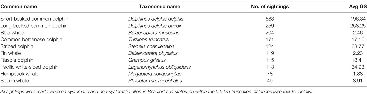
Table 2 Number of sightings and average group size (Avg GS) of cetacean species observed in the Southern California Current study area during the 1992–2018 shipboard surveys for which habitat-based density models were developed.

Correction factors for unidentified large whales were applied separately by Beaufort sea state for the 2018 blue, fin, and humpback whale sightings, because the proportion of unidentified whales increased with increasing sea state. For blue and humpback whales, these correction factors were 1.03, 1.04, 1.05, 1.20, and 1.26 for Beaufort sea states 0-1, 2, 3, 4, and 5, respectively, and 1.04, 1.08, 1.10, 1.30, and 1.46 for fin whales. Correction factors for unidentified common dolphins did not increase with increasing sea states, so a uniform correction factor of 1.71 was applied across all sea states for the 2018 sightings of both long- and short-beaked common dolphins.

The functional forms of the key predictor variables were consistent with those of SDMs built for waters off the U.S. West Coast (Becker et al., 2016; Becker et al., 2018; Becker et al., 2020b; Supplementary Material). Depth was the most common predictor variable included in the encounter rate models of groups (long- and short-beaked common dolphins) or individuals (all other species), and was selected in all but the sperm whale model (Table 3). Differences in depth-defined habitat are clearly evident in the predicted density plots for long-beaked common dolphin, Pacific white-sided dolphin, and humpback whale, three species occurring primarily in coastal shallow-water habitat (Figures 3A, D, J), and striped dolphin, a species found in the deep, offshore waters of the study area (Figure 3E). SST and SSTsd were the most commonly selected dynamic predictor variables, followed closely by SAL. The dynamic covariates generally exhibited unimodal, threshold, or linear relationships consistent with known patterns of distribution with the broader California Current Ecosystem (Supplementary Material). Consistent with other studies that have demonstrated significant spatial variation in group size, particularly for delphinids (Ferguson et al., 2006; Barlow, 2015), the group size model for both subspecies of common dolphin included a bivariate spline of longitude and latitude.

TABLE 3

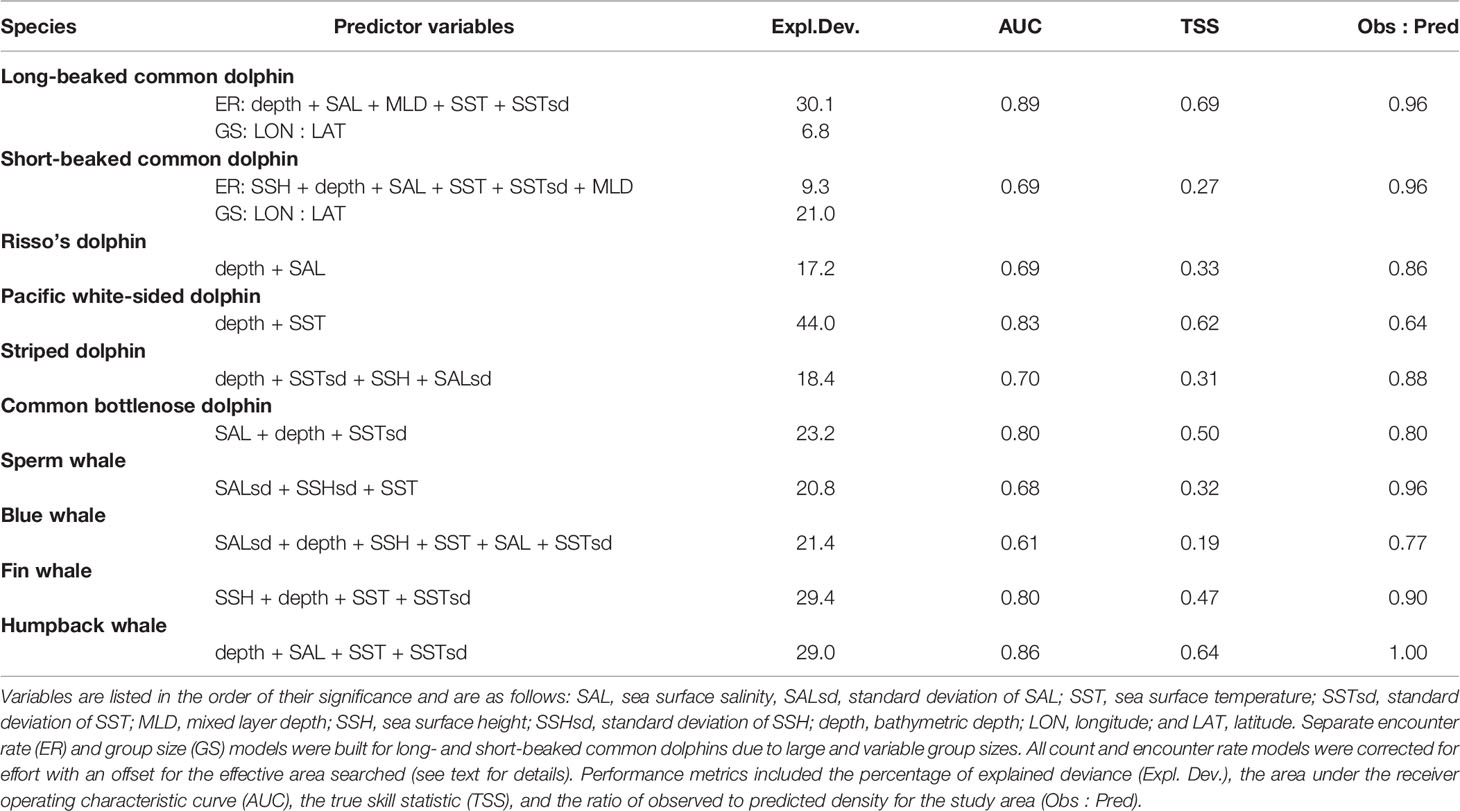
Table 3 Summary of the final models built with the 1992–2018 survey data.

3.2 Model Performance

Deviance explained by the models was variable among the species, ranging from approximately 17% (Risso’s dolphin) to 44% (Pacific white-sided dolphin; Table 3). AUC values for all models were greater than 0.6, indicating that the models exhibited better than random skill at predicting true positives and negatives. The TSS values, which account for both omission and commission errors, ranged from 0.19 (blue whale) to 0.69 (long-beaked common dolphin), also indicating performance was better than random (i.e., all values were >0). The observed: predicted density ratios provide an indication of how well the sum of the segment-based density predictions from the model compare to study area abundance as derived from design-based line-transect methods, and these values were close to 1.00 for most species (humpback whale, long-and short-beaked common dolphins, and sperm whale), and lowest (0.64) for Pacific white-sided dolphin (Table 3).

Comparison of the geographically stratified abundance estimates showed generally good agreement between the magnitude of model predicted and design-based estimates (Table 4). For most species, strata with the greatest and lowest density values were consistent between the two analytical methods, indicating that the models were effective at predicting spatial variability in abundance throughout the study area. There was exceptional agreement between the relative density estimates for short-beaked common dolphin, the species with the greatest number of sightings available for modeling (Tables 2, 4).

TABLE 4

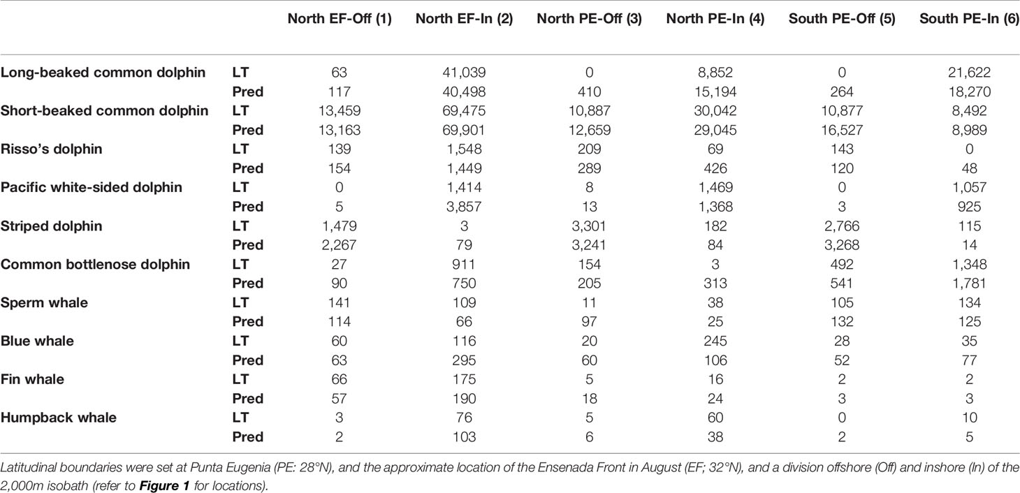
Table 4 Relative abundance (defined as the encounter rate multiplied by the group size, without correcting for detection probability) as predicted from the models (Pred) and derived from standard line-transect analyses (LT) for the six geographic strata defined for the Southern California Current study area.

3.3 Model Predictions

For the three species with previously hypothesized shifts in distribution in and out of U.S. waters (striped dolphins and short- and long-beaked common dolphins), there was variability evident in total year-to-year abundance within the Southern California Current study area, but not a clear inverse relationship between abundance north of 32°N compared to the southern region (Figure 2). However, total abundance of both short-beaked and striped dolphins was lowest in 2014, the year for which absolute abundance of both species increased off U.S. waters and their distributions shifted well north of 42°N latitude (Barlow, 2016; Becker et al., 2018).

FIGURE 2

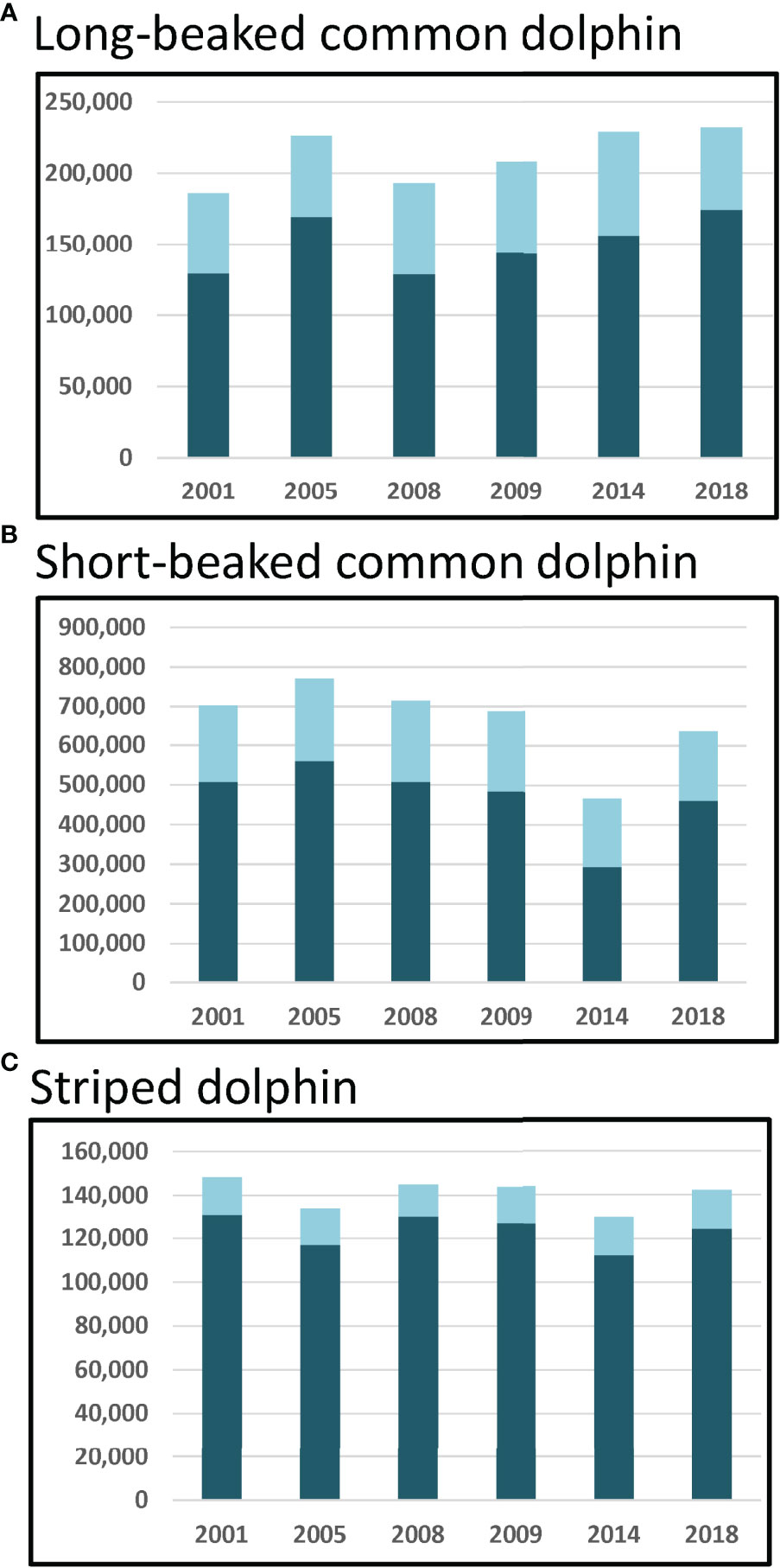
Figure 2 Total yearly abundance for the two strata north of 32°N (light blue) and the four strata south of 32°N (dark blue) as predicted from the 1992–2018 habitat-based density models for (A) long-beaked common dolphin, (B) short-beaked common dolphin, and (C) striped dolphin. Strata are shown in Figure 1.

With the exception of Risso’s dolphin, the 2001–2018 multi-year average density surface maps generally captured observed distribution patterns as illustrated by actual sightings during the surveys (Figure 3). The Risso’s dolphin model predicted greater densities in nearshore waters of the SCB, consistent with the sightings data, but appeared to overestimate offshore densities between the southern SCB and Punta Eugenia and underestimate densities south of Punta Eugenia (Figure 3C). The pixel-specific CVs, which incorporated uncertainty from the model parameters, ESW, and environmental variability of the daily 2001–2018 predictions, showed substantial variation among the species, with the largest individual pixel values in areas with few to no sightings and/or limited survey effort (e.g., Figures 3A, E).

FIGURE 3

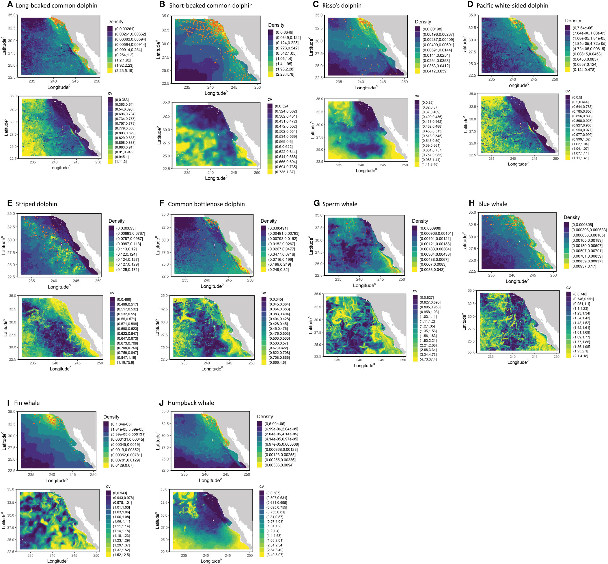
Figure 3 Predicted densities and uncertainty estimates from the 1992–2018 habitat-based density models for (A) long-beaked common dolphin, (B) short-beaked common dolphin, (C) Risso’s dolphin, (D) Pacific white-sided dolphin, (E) striped dolphin, (F) common bottlenose dolphin, (G) sperm whale, (H) blue whale, (I) fin whale, and (J) humpback whale. Panels show the multi-year average density based on predicted daily cetacean species densities covering the survey periods (summer/fall 2001–2018), as well as the coefficients of variation (CV) of density. The range of values represented by each color are shown to the right of the color block; in the average plots they represent the upper 1%, 2%, 5%, 10%, 25% 50%, 75%, 90%, and 100% of the species-specific density values, with the greatest value increased to encompass the greatest value predicted among the years (see text for details). Orange dots in the average plots show actual sighting locations from the SWFSC summer/fall ship surveys for the respective species.

Interannual variability in density and distribution was evident for all species between 2001 and 2018 (Figure 4). For the three warm-temperate species included in the study (striped dolphin and short- and long-beaked common dolphins), interannual variability was exhibited throughout the study area (Figures 4A, B, E). The region within and south of Bahia Sebastián Vizcaíno showed the greatest interannual variability in density for long-beaked common dolphin (Figure 4A), perhaps in part due to changing conditions south of our study area or within the Gulf of California where this species is also abundant. Short-beaked common dolphin also showed interannual variability in this region, in addition to notable variations within the Southern California Bight, particularly in 2014 when substantially lower densities were predicted (Figure 4B). Striped dolphin model predictions show moderate to high densities shifting annually off the shelf within the outer California Current Ecosystem (Figure 4E), although strong patterns are not discernible since the upper five density bins are so similar given the percentile scheme used to present density.

FIGURE 4

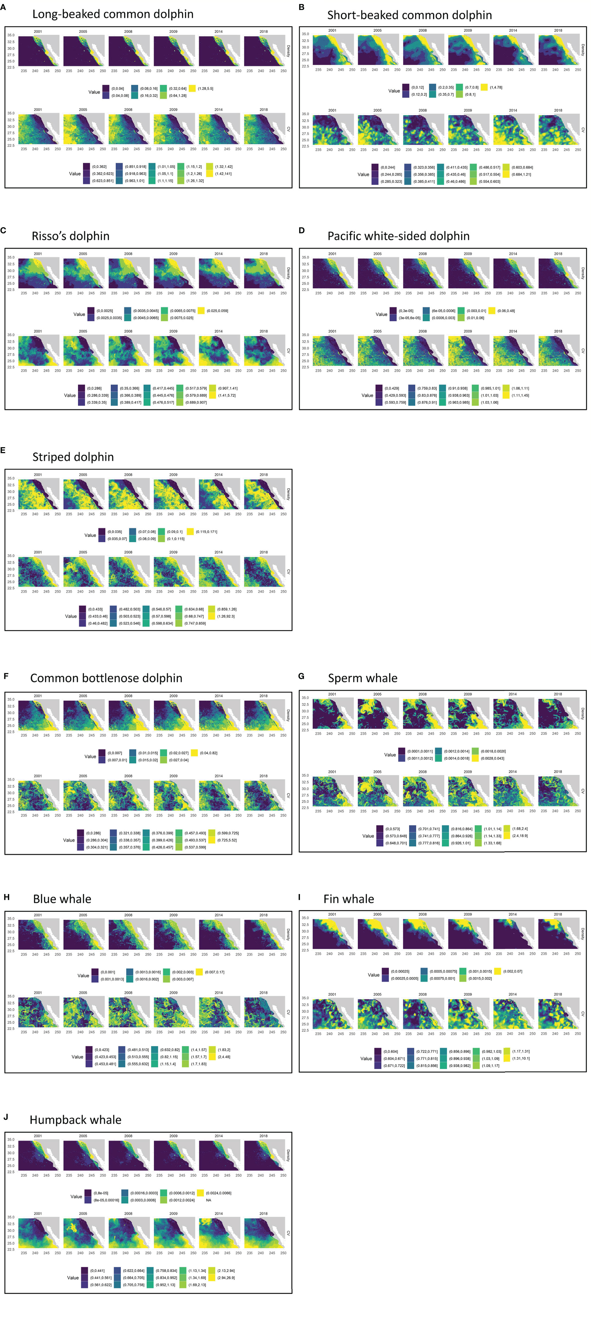
Figure 4 Predicted yearly (2001-2018) mean densities and uncertainty estimates from the 1992–2018 habitat-based density models for (A) long-beaked common dolphin, (B) short-beaked common dolphin, (C) Risso’s dolphin, (D) Pacific white-sided dolphin, (E) striped dolphin, (F) common bottlenose dolphin, (G) sperm whale, (H) blue whale, (I) fin whale, and (J) humpback whale. Panels show the yearly average density based on predicted daily cetacean species densities covering August-November of the respective years, as well as the coefficients of variation of density (CV). The range of values represented by each color are shown to the right of the color block. Density ranges are the same as those used for the 1992–2018 average density estimates shown in Figure 3.

The interannual density predictions for Risso’s dolphin showed variable distribution patterns throughout the study area, but given the poor performance revealed by the multi-average plot for this species, it is not clear how reliable these predictions are, particularly south of Punta Eugenia (Figure 4C). Interannual variability in density in both U.S. and Mexican waters was evident for all three species of mysticetes, whose migration paths encompass the full range of the Southern California Current study area (Figures 4H-J). The yearly average density plots for Pacific white-sided dolphin showed greatest variability along the coast and around Bahia Sebastián Vizcaíno, with the southerly extent of highest density expanding and contracting from year to year (Figure 4D). Substantial interannual variability along the coast was also apparent for common bottlenose dolphin, particularly south of Punta Eugenia (Figure 4F). The yearly density plots for sperm whales show two main areas of high density, one in the northwest portion of the study area and another in the southeast portion of the study area off the southern Baja California peninsula, with the extent of highest predicted density shifting on an interannual basis (Figure 4G).

4 Discussion

The SDMs developed in this study provide the first fine-scale (9 x 9 km grid) estimates of average cetacean species density and abundance in summer/fall for waters west of the Baja California peninsula, México, and will support efforts to assess and mitigate anthropogenic impacts. This analysis also provides spatially-explicit measures of uncertainty that account for the major known sources of SDM variance (environmental variability, ESW, and model parameters). The largest CVs were generally located in the southwestern portion of the study area where survey effort was sparse and there is likely still unresolved uncertainty (Figures 1, 3). Incorporating additional systematic survey data from this region into future SDMs would help to improve predictions for this area, particularly if data were collected during winter/spring, when cetacean distribution patterns could be markedly different (Becker et al., 2017).

Sample sizes were sufficient to develop SDMs for ten taxonomically diverse species: three warm temperate species (long-beaked common, short-beaked common, and striped dolphins), one cold temperate species (Pacific white-sided dolphin), three cosmopolitan species (Risso’s dolphin, common bottlenose dolphin, and sperm whale), and three migratory large whales (blue, fin, and humpback whales). Over the last 20 years, SDMs for these species have been developed for U.S. West Coast waters using much of the survey data used for this study (Forney, 2000; Barlow et al., 2009; Becker et al., 2010; Forney et al., 2012; Becker et al., 2014; Becker et al., 2016; Becker et al., 2018; Becker et al., 2020b). These analyses have enhanced our knowledge of spatial and temporal changes in species distribution off the U.S. West Coast, and more recently demonstrated the ability of SDMs to predict substantial changes in abundance and distribution when waters off the U.S. West Coast were anomalously warm (Becker et al., 2018). The performance of the SDMs developed in this study varied by species, and thus the models’ ability to predict interannual distribution patterns and capture previously documented shifts within the study area are discussed separately for each of the major species groups below.

4.1 Warm Temperate Dolphins

Becker et al. (2018) showed that in 2014, when an unprecedented marine heatwave spread over the area (Bond et al., 2015; Leising et al., 2015; Di Lorenzo and Mantua, 2016), the distributions of both short-beaked common and striped dolphin shifted north of 42°N, atypical of previous observations, and the abundance of both species increased substantially. This finding was consistent with previous studies that hypothesized that the large interannual variation in abundance of the warm temperate delphinids in U.S. West Coast waters is largely due to distribution shifts between U.S. and Mexican waters (Dohl et al., 1986; Heyning and Perrin, 1994; Forney and Barlow, 1998; Barlow, 2016).

Based on the SDMs developed for this study, the distributions of both short-beaked common and striped dolphins shifted north in 2014, and abundance in the Southern California Current study area was the lowest of all years considered (Table 5; Figures 2, 4B, E). The 2014 abundance estimate for short-beaked common dolphin north of 32°N was lower than the other years (172,873 dolphins in 2014 compared to a range of 175,412–211,121), and south of 32°N was notably lower (293,224 dolphins in 2014 compared to a range of 461,285–559,478 dolphins in the other years; Figure 2). Becker et al. (2018) found the 2014 abundance of short-beaked common dolphins within the entire U.S. EEZ study area to be greater than the 1991–2009 average. Taken together, results from this and the Becker et al. (2018) study provide evidence that in 2014, there was a large distribution shift of short-beaked common dolphins northward out of Mexican waters into U.S. West Coast waters extending well north of 32°N during the anomalously warm year.

TABLE 5

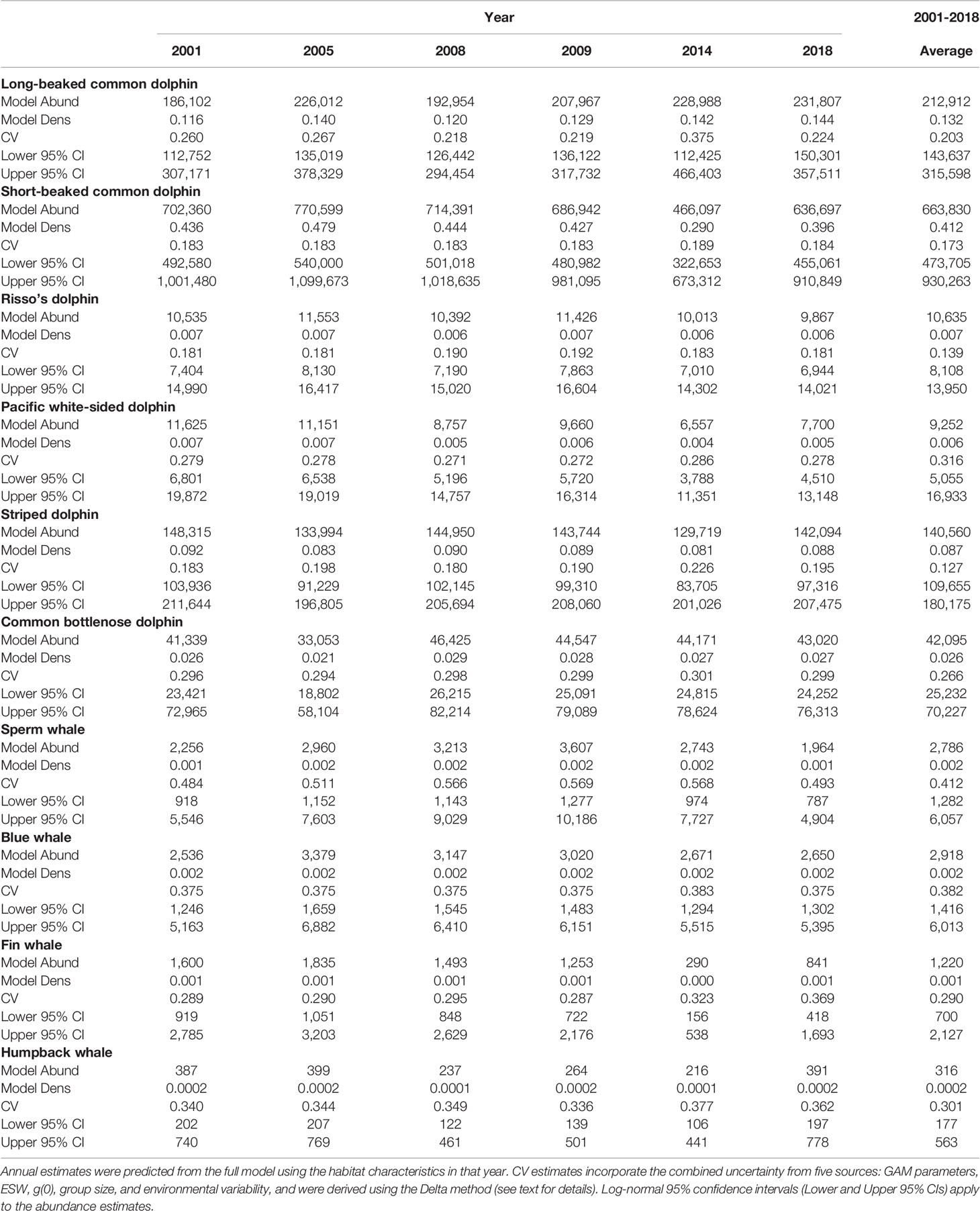
Table 5 Annual and multi-year (2001–2018) model-predicted mean estimates of abundance (Abund), density (Dens; animals km-2), and corresponding coefficient of variation (CV) within the Southern California Current study area

Similar to short-beaked common dolphin but less striking, the regionally-stratified 2014 abundance estimates for striped dolphin also suggest that this species’ distribution shifted north from Mexican waters into U.S. West Coast waters during the warm year. Striped dolphin abundance north of 32°N was estimated in this study to be similar during 2014 and other years, but south of 32°N it was lowest during 2014 (112,344 dolphins compared to a range of 117,067–130,082 dolphins in the other years; Figure 2). Despite similar abundance estimates for the Southern California Current study area among years (Table 5; Figure 2), annual distribution patterns appear to expand and contract in both a northeast-southwest direction (Figure 4E; e.g., compare expansion in 2001 to contraction in 2005). These shifts would likely affect the abundance of striped dolphins in offshore U.S. West Coast waters. Becker et al. (2018) found the 2014 abundance of striped dolphins to be greater than the 1991–2009 average in U.S. West Coast waters, but primarily north of 32°N. The density predictions from this study are consistent with this finding, as there were lower numbers of dolphins in the Southern California Current study area in 2014 (Figure 4E), when greater numbers were observed in offshore waters north of Point Conception (Becker et al., 2018).

Long-beaked common dolphin is another warm-temperate species thought to move north from Mexican waters into U.S. West Coast waters when ocean conditions warm (Heyning and Perrin, 1994; Forney and Barlow, 1998; Barlow, 2016). Occurring primarily in coastal waters, the range of long-beaked common dolphin typically extends from central California south along the Baja California peninsula, and up into the Gulf of California (Gerrodette and Eguchi, 2011). Becker et al. (2020a) found the abundance of long-beaked common dolphins in waters off the U.S. West Coast to be greater in the warm 2014 year than the average 1991–2009 abundance. Greater-than-average density was predicted throughout their typical range, including the coastal area of central California, where influxes of long-beaked common dolphins have previously been documented during warm-water El Niño years (Benson et al., 2002). Results from our study are consistent with this finding, as the model-predicted yearly abundance estimate for the two strata north of 32°N was greatest during 2014 (73,012 dolphins compared to 56,475–64,444 for the other years, Figure 2). Although an inverse relationship between strata north and south of 32°N is not apparent from this study, the lowest model-based abundance estimate for long-beaked common dolphin in the southern strata of the Southern California Current study area was in 2008 (Figure 2). Based on design-based abundance estimates for U.S. West Coast waters between 1996 and 2014, 2008 had the greatest number of long-beaked common dolphins (114,031, CV=0.88), exceeding the point estimate for 2014 (89,998, CV=0.58; Barlow, 2016). Combined, these results suggest that in both 2008 and 2014 there were northern shifts in long-beaked common dolphin distribution from Mexican into U.S. West Coast waters, likely driven by environmental variability. Data collected within the full range of their distribution, including the Gulf of California, may be necessary to capture more subtle long-beaked common dolphin distribution shifts not apparent from the data available for this study.

4.2 Migratory Large Whales

The model-predicted 2014 abundance estimate for fin whales was markedly lower than in other years (Table 5), with the 2014 estimate (290 whales) below the lower 95% confidence intervals of the other years. The interannual density plots for this species also show obvious differences in 2014, with the greatest predicted densities concentrated in the northern portion of the study area, primarily within U.S. West Coast waters (Figure 4I). Fin whales are known to occur year-round off southern California, with a seasonal influx of migratory whales along the entire U.S. West Coast (Dohl et al., 1980; Barlow, 1994; Forney et al., 1995, Forney and Barlow, 1998; Campbell et al., 2015). Both design- and model-based analyses (Barlow, 2016; Becker et al., 2018) estimated an increase in fin whale abundance in waters off the U.S. West Coast in 2014, including both waters off southern California and areas as far north as Oregon. A similar northward shift of fin whales along the U.S. West Coast was previously documented during the warm-water year of 2005 (Peterson et al., 2006). Thus, the decreased abundance of fin whales in waters west of the Baja California peninsula identified in this study during 2014 is consistent with other studies showing a northward shift during warm years.

The 2014 model-predicted abundance estimate for humpback whales in the Southern California Current study area was also the lowest of the years considered in this study (Table 5). Similar to fin whale, both design- and model-based analyses estimated greater than average humpback whale abundance in waters off the U.S. West Coast in 2014, with the largest densities predicted for coastal waters of central California, north of 32°N (Barlow, 2016; Becker et al., 2018). This suggests that during the 2014 warm year, when there were large numbers of humpback whales off the U.S. West Coast, fewer humpback whales were in waters west of the Baja California peninsula. The interannual density plots for this species show high variability in abundance along the Baja peninsula, particularly within Bahia Sebastián Vizcaíno (Figure 4J; e.g., compare 2005 and 2008). Interannual pixel-specific CVs are also quite variable, although areas of greatest uncertainty are generally in the south and offshore, areas with the fewest sightings (Figure 4J).

Model-predicted blue whale densities also show large interannual variability throughout the Southern California Current study area (Figure 4H). Analysis of systematic survey data collected between 1991 and 2014 suggests a northward shift of blue whale distribution in waters off the U.S. West Coast due to warming ocean temperatures (Barlow and Forney, 2007; Calambokidis et al., 2009; Barlow, 2016). Interestingly, blue whale abundance estimates for the Southern California Current study area decreased from 2005 to 2014, but showed a slight increase in 2018 (Table 5). The 2018 density plot for blue whale shows an increase in the greatest densities along the coast of the Baja California peninsula, particularly south of Punta Eugenia, an area characterized by much lower densities from 2008-2014 (Figure 4H).

4.3 Cool Temperate/Cosmopolitan Species

Interannual variability in the density patterns for Pacific white-sided dolphin were also evident, mainly off the Baja peninsula, where clear north-south shifts in distribution are apparent (Figure 4D). A cool temperate species, it has been suggested that Pacific white-sided dolphin distribution shifts both seasonally and interannually off the U.S. West Coast, with animals moving north into waters off Oregon and Washington during warm conditions and moving south into California waters during cool conditions (Green et al., 1992; Forney and Barlow, 1998; Becker et al., 2014; Barlow, 2016). A decline in the presence of Pacific white-sided dolphins in the southwest Gulf of California, considered the southern boundary of this species range, has been attributed to warming ocean temperatures (Salvadeo et al., 2010). The interannual density plots suggest that the greatest north-south shift along the Baja California coast occurred during 2014, when densities south of Punta Eugenia were lower than in other years. Given that 2014 was considered an anomalous warm year, this result is consistent with those of previous studies.

Pacific white-sided dolphins that occur in waters west of the Baja California peninsula are genetically different from those occurring off central California to Washington, with the SCB representing a variable mixing zone for the two forms (Lux et al., 1997). Two types of echolocation have been documented for Pacific white-sided dolphins off Southern California, suggesting acoustic differences between the two forms (Soldevilla et al., 2008; Soldevilla et al., 2010; Henderson et al., 2011). The relative abundance estimates for Pacific white-sided dolphins were quite good for every area except the SCB (Table 4), which is precisely the mixing area for the two forms, suggesting that perhaps there are some habitat differences for these two forms that are confounding the models.

The interannual density predictions for Risso’s dolphin showed fairly consistent distribution patterns in the northern portion of the study area, except for 2018, when densities were much lower everywhere except nearshore along the coast (Figure 4C). Substantial onshore-offshore shifts of moderate density were apparent between about 29–32°N. However, it is difficult to determine how real these distribution patterns are, since the average density plot did not match the sighting data well (Figure 3C). SDMs developed for Risso’s dolphin off the U.S. West Coast have historically exhibited poor performance (Becker et al., 2010; Forney et al., 2012), although a model developed in a recent study was able to predict the observed spatial patterns quite well (Becker et al., 2020b).

Two bottlenose dolphin ecotypes are known to occur within the Southern California Current study area, an offshore form and a coastal form that occurs primarily within 1 km from shore (Carretta et al., 1998; Defran and Weller, 1999). Given the locations of bottlenose dolphin sightings used in this analysis, they are considered to be the offshore form. The interannual density plots for common bottlenose dolphin show very similar distribution patterns north of Punta Eugenia, but greater variation is apparent offshore of the southern Baja California peninsula, in the southernmost portion of the study area (Figure 4F). In this area, the regions of greatest density appear to shift both north-south and inshore-offshore inter-annually, suggesting that shifting distributions may be driven by oceanic changes in this region.

Sperm whales exhibited a large degree of interannual variation in density throughout the study area (Figure 4G), with a swath of low density that changes in location and extent from year to year. The multi-year average density plot for sperm whale shows the low-density swath extending SSW from nearshore southern California waters, effectively separating the areas of greater density (Figure 3G). The multi-year average density map captures the distribution of actual survey sightings well; however, the low-density swath also coincides with the region of lowest survey coverage (Figure 1). Additional data are needed to resolve whether this low-density region has a true ecological basis.

4.4 Summary

When considering all the species combined, the modeling approach worked well, consistent with similar SDMs developed for waters off the U.S. West Coast (Becker et al., 2016; Becker et al., 2018; Becker et al., 2020a; Becker et al., 2020b). Interannual distribution patterns were generally consistent with those documented in past regional studies, but the broader study range addressed in this study provided a “bigger picture” view of the Southern California Current ecosystem. Models developed for the warm temperate dolphins, cool temperate Pacific white-sided dolphin, and large migratory whales exhibited the strongest model performance in terms of concordance between density predictions and survey sightings. Reasonable concordance was also seen for the cosmopolitan bottlenose dolphin and sperm whale models, although the sample size for the latter was limited (49 sightings), thus reducing the degree of confidence in the predicted density patterns. Model performance was the worst for Risso’s dolphin, another cosmopolitan species for which past SDMs have also exhibited poor performance, suggesting that the environmental covariates were not effective proxies for their habitat or prey (Becker et al., 2020a). The quantitative spatial data derived from these SDMs provide management tools useful for assessing and mitigating potential anthropogenic impacts, and reaffirm the importance of assessing and managing cetaceans at biologically relevant spatial scales, particularly in a changing climate.

5 Conclusions

The dynamic cetacean SDMs developed in this study provide multi-year average summer/fall density surfaces for stakeholders to use in their long-term environmental planning efforts. The modeled predictions represent a major improvement over density estimates currently used for management purposes in waters west of the Baja California peninsula, México, because they provide finer-scale density predictions (9 x 9 km grid resolution vs. the current 5° X 5° grid resolution) and improved, spatially-explicit estimates of uncertainty. The model predictions provide insight into our understanding of species distribution patterns by including a broader distribution range of many species, and document previously known interannual movements within the California Current Ecosystem that are centered in the SCB. For the warm temperate species suspected to exhibit distribution shifts between U.S. and Mexican waters (striped, and long- and short-beaked common dolphins), northern distribution shifts were apparent during the anomalously warm conditions in 2014, when densities decreased off the southern Baja California peninsula. More subtle distribution shifts were not apparent, perhaps due to a need for finer scale data or because the ecological context may be more complex than the relationships captured by the SDMs. Interannual variability in density and distribution were apparent for the other species as well, including the migratory whale species, but additional data are needed to resolve some of the patterns identified by the model predictions. Data collected in winter/spring are needed to estimate density in these seasons, when cetacean distribution patterns could be quite different from summer/fall. Efforts aimed at improving the explanatory and predictive performance of the SDMs developed in this study will help to support the conservation of cetacean species that have continuous distributions between U.S., Mexican, and international waters, and may lead to improved cooperative management strategies across jurisdictional boundaries in this region.

Data Availability Statement

The datasets presented in this study can be found in online repositories. The names of the repository/repositories and accession number(s) can be found below: The cetacean data used in this study are publicly available on the Cetacean and Sound Mapping website (https://cetsound.noaa.gov/cda). The hybrid coordinate ocean model (HYCOM) output is publicly available on the HYCOM Catalog website (http://ncss.hycom.org/thredds/catalog.html). Further inquires can be directed to the corresponding author.

Ethics Statement

Ethical review and approval was not required for the animal study because our research used sighting data collected during ship surveys that were conducted under all relevant permits.

Author Contributions

EB, KF, JB, and JM conceived the ideas and interpreted the results with input from DM, LRB, and JUR. EB, KF, and DM contributed to model development. EB and KF processed the cetacean survey data. JB, KF and JM designed, conducted, and contributed the cetacean survey data. EB led the analysis and writing, and all authors participated in writing and revising the manuscript. All authors read and approved the final manuscript.

Funding

This modeling project was funded by the Navy, Commander, U.S. Pacific Fleet (U.S. Navy), the Bureau of Ocean Energy Management (BOEM), and by the National Oceanic and Atmospheric Administration (NOAA), National Marine Fisheries Service (NMFS), Southwest Fisheries Science Center (SWFSC). The 2018 survey was conducted as part of the Pacific Marine Assessment Program for Protected Species (PacMAPPS), a collaborative effort between NOAA Fisheries, the U.S. Navy, and BOEM to collect data necessary to produce updated abundance estimates for cetaceans in the CCE study area. BOEM funding was provided via Interagency Agreement (IAA) M17PG00025, and Navy funding via IAA N0007018MP4C560, under the Mexican permit SEMARNAT/SGPA/DGVS/013212/18. The methods used to derive uncertainty estimates were developed as part of “DenMod: Working Group for the Advancement of Marine Species Density Surface Modeling” funded by OPNAV N45 and the SURTASS LFA Settlement Agreement, and managed by the U.S. Navy’s Living Marine Resources (LMR) program under Contract No. N39430-17-C-1982. Other permits included INEGI: Oficio núm. 400./331/2018, INEGI.GMA 1.03 SAGARPA de Oficio B00.02.04.1530/2018 NMFS Permit No. 19091.

Conflict of Interest

EB is employed by ManTech International Corporation.

The remaining authors declare that the research was conducted in the absence of any commercial or financial relationships that could be construed as a potential conflict of interest.

Publisher’s Note

All claims expressed in this article are solely those of the authors and do not necessarily represent those of their affiliated organizations, or those of the publisher, the editors and the reviewers. Any product that may be evaluated in this article, or claim that may be made by its manufacturer, is not guaranteed or endorsed by the publisher.

Acknowledgments

The survey data used in this analysis were collected by a dedicated team from NOAA’s Southwest Fisheries Science Center (SWFSC) and we thank everyone who contributed to collecting these data. Chief Scientists for the ship surveys included Lisa Ballance, Tim Gerrodette, Susan Chivers, and three of the co-authors (JB, JM, and KF). This report was improved by the helpful reviews of Jim Carretta, Chip Johnson, and Sean Hanser.

Supplementary Material

The Supplementary Material for this article can be found online at: https://www.frontiersin.org/articles/10.3389/fmars.2022.829523/full#supplementary-material

References

Abrahms B., Welch H., Brodie S., Jacox M. G., Becker E. A., Bograd S. J., et al. (2019). Dynamic Ensemble Models to Predict Distributions and Anthropogenic Risk Exposure for Highly Mobile Species. Diversity Distrib. 25 (8), 1182–1193. doi: 10.1111/ddi.12940

CrossRef Full Text | Google Scholar

Allouche O., Tsoar A., Kadmon R. (2006). Assessing the Accuracy of Species Distribution Models: Prevalence, Kappa and the True Skill Statistic (Tss). J. Appl. Ecol. 43 (6), 1223–1232. doi: 10.1111/j.1365-2664.2006.01214.x

CrossRef Full Text | Google Scholar

Amante C., Eakins B. W. (2009). “ETOPO1 1 Arc-Minute Global Relief Model: Procedures, Data Sources and Analysis,” in NOAA Technical Memorandum NESDIS NGDC-24 (Boulder, CO: National Geophysical Data Center).

Google Scholar

Barlow J. (1994). “Recent Information on the Status of Large Whales in California Waters,” in NOAA Technical Memorandum NMFS-SWFSC-203 (La Jolla, CA, USA: National Marine Fisheries Service).

Google Scholar

Barlow J. (1995). The Abundnace of Cetaceans in California Waters: Part I: Ship Surveys in the Summer and Fall of 1991. Fisher. Bull. 93, 1–14.

Google Scholar

Barlow J. (1997). “Preliminary Estimates of Cetacean Abudance Off California, Oregon, and Washington Based on a 1996 Ship Survey and Comparisons of Passing and Closing Modes,” in Administrative Report LJ-97-11, NMFS-SWFSC (La Jolla, CA, USA: National Marine Fisheries Service).

Google Scholar

Barlow J. (2015). Inferring Trackline Detection Probabilities, G(0), for Cetaceans From Apparent Densities in Different Survey Conditions. Mar. Mamm. Sci. 31, 923–943. doi: 10.1111/mms.12205

CrossRef Full Text | Google Scholar

Barlow J. (2016). “Cetacean Abundance in the California Current Estimated From Ship-Based Line-Transect Surveys in 1991-2014,” in NOAA Administrative Report LJ-16-01 (La Jolla, CA, USA: National Marine Fisheries Service).

Google Scholar

Barlow J., Ballance L. T., Forney K. A. (2011). “Effective Strip Widths for Ship-Based Line-Transect Surveys of Cetaceans,” in NOAA Technical Memorandum NMFS-SWFSC-484 (La Jolla, CA, USA: National Marine Fisheries Service).

Google Scholar

Barlow J., Ferguson M. C., Becker E. A., Redfern J. V., Forney K. A., Vilchis I. L., et al. (2009). “Predictive Modeling of Cetacean Densities in the Eastern Pacific Ocean,” in NOAA Technical Memorandum NMFS-SWFSC-444 (La Jolla, CA, USA: National Marine Fisheries Service).

Google Scholar

Barlow J., Forney K. A. (2007). Abundance and Population Density of Cetaceans in the California Current Ecosystem. Fisher. Bull. 105, 509–526.

Google Scholar

Barlow J., Gerrodette T., Forcada J. (2001). Factors Affecting Perpendicular Sighting Distances on Shipboard Line-Transect Surveys for Cetaceans. J. Cetac. Res. Manage. 3, 201–212.

Google Scholar

Becker E. A., Carretta J. V., Forney K. A., Barlow J., Brodie S., Hoopes R., et al. (2020a). Performance Evaluation of Cetacean Species Distribution Models Developed Using Generalized Additive Models and Boosted Regression Trees. Ecol. Evol. 10, 5759–5578. doi: 10.1002/ece3.6316

PubMed Abstract | CrossRef Full Text | Google Scholar

Becker E. A., Forney K. A., Ferguson M. C., Foley D. G., Smith R. C., Barlow J., et al. (2010). Comparing California Current Cetacean-Habitat Models Developed Using In Situ and Remotely Sensed Sea Surface Temperature Data. Mar. Ecol. Prog. Ser. 413, 163–183. doi: 10.3354/meps08696

CrossRef Full Text | Google Scholar

Becker E. A., Forney K. A., Fiedler P. A., Barlow J., Chivers S. J., Edwards C. A., et al. (2016). Moving Towards Dynamic Ocean Management: How Well do Modeled Ocean Products Predict Species Distributions? Remote Sens. 8, 149. doi: 10.3390/rs8020149

CrossRef Full Text | Google Scholar

Becker E. A., Forney K. A., Foley D. G., Smith R. C., Moore T. J., Barlow J. (2014). Predicting Seasonal Density Patterns of California Cetaceans Based on Habitat Models. Endanger. Species. Res. 23, 1–22. doi: 10.3354/esr00548

CrossRef Full Text | Google Scholar

Becker E. A., Forney K. A., Miller D. L., Fiedler P. C., Barlow J., Moore J. E. (2020b). “Habitat-Based Density Estimates for Cetaceans in the California Current Ecosystem Based on 1991–2018 Survey Data,” in U.S. Dept. Of Commerce, NOAA Technical Memorandum NOAA-TM-NMFS-SWFSC-638 (La Jolla, CA, USA: National Marine Fisheries Service), 78.

Google Scholar

Becker E. A., Forney K. A., Redfern J. V., Barlow J., Jacox M. G., Roberts J. J., et al. (2018). Predicting Cetacean Abundance and Distribution in a Changing Climate. Diversity Distrib. 43, 459–418. doi: 10.1111/ddi.12867

CrossRef Full Text | Google Scholar

Becker E. A., Forney K. A., Thayre B. J., Debich A. J., Campbell G. S., Whitaker K., et al. (2017). Habitat-Based Density Models for Three Cetacean Species Off Southern California Illustrate Pronounced Seasonal Differences. Front. Mar. Sci. 4. doi: 10.3389/fmars.2017.00121

CrossRef Full Text | Google Scholar

Benson S. R., Croll D. A., Marinovic B., Chavez F. P., Harvey J. T. (2002). Changes in the Cetacean Assemblage of a Coastal Upwelling Ecosystem During El Niño 1997-98 and the La Niña 1999. Prog. Oceanog. 54, 279–291. doi: 10.1016/S0079-6611(02)00054-X

CrossRef Full Text | Google Scholar

Bond N. A., Cronin M. F., Freeland H., Mantua N. (2015). Causes and Impacts of the 2014 Warm Anomaly in the NE Pacific. Geophys. Res. Lett. 42, 3414–3420. doi: 10.1002/2015GL063306

CrossRef Full Text | Google Scholar

Boyd C., Barlow J., Becker E. A., Forney K. A., Gerrodette T., Moore J. E., et al. (2018). Estimation of Population Size and Trends for Highly Mobile Species With Dynamic Spatial Distributions. Diversity Distrib. 24, 1–12. doi: 10.1111/ddi.12663

CrossRef Full Text | Google Scholar

Briggs J. C. (1974). Marine Zoography (New York, NY: McGraw-Hill).

Google Scholar

Buckland S. T., Anderson D. R., Burnham K. P., Laake J. L., Borchers D. L., Thomas L. (2001). Introduction to Distance Sampling: Estimating Abundance of Biological Populations (Oxford, U.K: Oxford University Press).

Google Scholar

Calambokidis J., Barlow J., Ford J. K. B., Chandler T. E., Douglas A. B. (2009). Insights Into the Population Structure of Blue Whales in the Eastern North Pacific From Recent Sightings and Photographic Identification. Mar. Mamm. Sci. 25, 816–832. doi: 10.1111/j.1748-7692.2009.00298.x

CrossRef Full Text | Google Scholar

Campbell G. S., Thomas L., Whitaker K., Douglas A. B., Calamboikdis J., Hildebrand J. A. (2015). Inter-Annual and Seasonal Trends in Cetacean Distribution, Density and Abundance Off Southern California. Deep. Sea. Res. Part II. 112, 143–157. doi: 10.1016/j.dsr2.2014.10.008

CrossRef Full Text | Google Scholar

Cañadas A., Hammond P. S. (2008). Abundance and Habitat Preferences of the Short-Beaked Common Dolphin Delphinus Delphis in the Southwestern Mediterranean: Implications for Conservation. Endanger. Species. Res. 4, 309–331. doi: 10.3354/esr00073

CrossRef Full Text | Google Scholar

Carretta J. V., Chivers S. J., Perryman W. L. (2011). Abundance of the Long-Beaked Common Dolphin (Delphinus Capensis) in California and Western Baja California Waters Estimated From a 2009 Ship-Based Line-Transect Survey. Bull. South. Califor. Acad. Sci. 110, 152–164. doi: 10.3160/0038-3872-110.3.152

CrossRef Full Text | Google Scholar

Carretta J. V., Forney K. A., Laake J. L. (1998). Abundance of Southern California Coastal Bottlenose Dolphins Estimated From Tandem Aerial Surveys. Mar. Mamm. Sci. 14 (4), 655–675. doi: 10.1111/j.1748-7692.1998.tb00755.x

CrossRef Full Text | Google Scholar

Chassignet E., Hulbert H., Smedstad O., Halliwell G., Hogan P., Wallcraft A., et al. (2007). The Hycom (Hybrid Coordinate Ocean Model) Data Assimilative System. J. Mar. System. 65, 60–83. doi: 10.1016/j.jmarsys.2005.09.016

CrossRef Full Text | Google Scholar

Checkley D. M. Jr, Barth J. A. (2009). Patterns and Processes in the California Current System. Prog. Oceanog. 83, 49–64. doi: 10.1016/j.pocean.2009.07.028

CrossRef Full Text | Google Scholar

Defran R. H., Weller D. W. (1999). Occurrence, Distribution, Site Fidelity, and School Size of Bottlenose Dolphins (Tursiops Truncatus) Off San Diego, California. Mar. Mamm. Sci. 15 (2), 366–380. doi: 10.1111/j.1748-7692.1999.tb00807.x

CrossRef Full Text | Google Scholar

Desportes G., Hansen R. G., Pike D. (2019). Sightings Surveys in the North Atlantic: 30 Years of Counting Whales Vol. 11 (Tromsø, Norway: NAMMCO Scientific Publications). doi: 10.7557/3.11

CrossRef Full Text | Google Scholar

Di Lorenzo E., Mantua N. (2016). Multi-Year Persistence of the 2014/15 North Pacific Marine Heat Wave. Nat. Climate Change 6, 1042–1047. doi: 10.1038/NCLIMATE3082

CrossRef Full Text | Google Scholar

Dohl T. P., Bonnell M. L., Ford R. G. (1986). Distribution and Abundance on Common Dolphin, Delphinus Delphis, in the Southern California Bight: A Quantitative Assessment Based Upon Aerial Transect Data. Fisher. Bull. 84, 333–343.

Google Scholar

Dohl T. P., Norris K. S., Guess R. C., Bryant J. D., Honig M. W. (1980). Summary of Marine Mammal and Seabird Surveys of the Southern California Bight Area 1975-78, Vol. III: Investigators’ Reports, Part II: Cetacea of the Southern California Bight (NTIS Catalog No. PB81-248189: Final Report to the Bureau of Land Management).

Google Scholar

Doyle R. F. (1985). Biogeographical Studies of Rocky Shore Near Point Conception, California. PhD dissertation (Santa Barbara, CA: University of California).

Google Scholar

Durazo R. (2015). Seasonality of the Transitional Region of the California Current System Off Baja California. J. Geophys. Res.: Ocean. 120, 1173–1196. doi: 10.1002/2014JC010405

CrossRef Full Text | Google Scholar

Fawcett T. (2006). An Introduction to ROC Analysis. Pattern Recog. Letter. 27 (8), 861–874. doi: 10.1016/j.patrec.2005.10.010

CrossRef Full Text | Google Scholar

Ferguson M. C., Barlow J. (2003). “Addendum: Spatial Distribution and Density of Cetaceans in the Eastern Tropical Pacific Ocean Based on Summer/Fall Research Vessel Surveys in 1986–96,” in U.S. Department of Commerce NOAA Administrative Report LJ-01-04 (La Jolla, CA: Southwest Fisheries Science Center).

Google Scholar

Ferguson M. C., Barlow J., Fiedler P. C., Reilly S. B., Gerrodette T. (2006). Spatial Models of Delphinid (Family Delphinidae) Encounter Rate and Group Size in the Eastern Tropical Pacific Ocean. Ecol. Modell. 193, 645–662. doi: 10.1016/j.ecolmodel.2005.10.034

CrossRef Full Text | Google Scholar

Forney K. A. (2000). Environmental Models of Cetacean Abundance: Reducing Uncertainty in Population Trends. Conserv. Biol. 14, 1271–1286. doi: 10.1046/j.1523-1739.2000.99412.x

CrossRef Full Text | Google Scholar

Forney K. A., Barlow J. (1998). Seasonal Patterns in the Abundance and Distribution of California Cetacean-1992. Mar. Mamm. Sci. 14, 460–489. doi: 10.1111/j.1748-7692.1998.tb00737.x

CrossRef Full Text | Google Scholar

Forney K. A., Barlow J., Carretta J. V. (1995). The Abundance of Cetaceans in California Waters. Part II: Aerial Surveys in Winter and Spring of 1991 and 1992. Fisher. Bull. 93, 15–26.

Google Scholar

Forney K. A., Becker E. A., Foley D. G., Barlow J., Oleson E. M. (2015). Habitat-Based Models of Cetacean Density and Distribution in the Central North Pacific. Endanger. Species. Res. 27, 1–20. doi: 10.3354/esr00632

CrossRef Full Text | Google Scholar

Forney K. A., Ferguson M. C., Becker E. A., Fiedler P. C., Redfern J. V., Barlow J., et al. (2012). Habitat-Based Spatial Models of Cetacean Density in the Eastern Pacific Ocean. Endanger. Species. Res. 16, 113–133. doi: 10.3354/esr00393

CrossRef Full Text | Google Scholar

Gerrodette T., Eguchi T. (2011). Precautionary Design of a Marine Protected Area Based on a Habitat Model. Endanger. Species. Res. 15, 159–166. doi: 10.3354/esr00369

CrossRef Full Text | Google Scholar

Green G. A., Brueggeman J. J., Grotefendt R. A., Bowlby C. E., Bonnell M. L., Balcomb K. C. III (1992). “Oregon and Washington: Marine Mammal and Seabird Survey. Chapter I: Cetacean Distribution and Abundance Off Oregon and Washington 1989-90,” (Los Angeles, California: OCS Study 91-0093, prepared for Pacific OCS Region, Minerals Management Service, U.S. Department of the Interior), xii + I00.

Google Scholar

Hamilton T. A., Redfern J. V., Barlow J., Balance L. T., Holt R. S., Forney K. A., et al. (2009). “Atlas of Cetacean Sightings for Southwest Fisheries Science Center Cetacean and Ecsystme Surveys: 1986-2005,” in NOAA Technical Memorandum NMFS-SWFSC-440 (La Jolla, CA, USA: National Marine Fisheries Service).

Google Scholar

Hammond P. S., Berggren P., Benke H., Borchers D. L., Collet A., Heide-Jørgensen M. P., et al. (2002). Abundance of Harbour Porpoises and Other Cetaceans in the North Sea and Adjacent Waters. J. Appl. Ecol. 39, 361–376. doi: 10.1046/j.1365-2664.2002.00713.x

CrossRef Full Text | Google Scholar

Hammond P. S., Lacey C., Gilles A., Viquerat S., Börjesson P., Herr H., et al. (2021). Estimates of Cetacean Abundance in European Atlantic Waters in Summer 2016 From the SCANS-III Aerial and Shipboard Surveys. Wagening. Mar. Res.

Google Scholar

Hammond P. S., Macleod K., Berggren P., Borchers D. L., Burt M. L., Cañadas A., et al. (2013). Cetacean Abundance and Distribution in European Atlantic Shelf Waters to Inform Conservation and Management. Biol. Conserv. 164, 107–122. doi: 10.1016/j.biocon.2013.04.010

CrossRef Full Text | Google Scholar

Hazen E. L., Palacios D. M., Forney K. A., Howell E. A., Becker E. A., Hoover A. L., et al. (2017). WhaleWatch: A Dynamic Management Tool for Predicting Blue Whale Density in the California Current. J. Appl. Ecol., 54 (5), 1–14. doi: 10.1111/1365-2664.12820

CrossRef Full Text | Google Scholar

Hedley S. L., Buckland S. T. (2004). Spatial Models for Line Transect Sampling. J. Agricul. Biolog. Environ. Stat. 9 (2), 181–199. doi: 10.1198/1085711043578

CrossRef Full Text | Google Scholar

Henderson E. E., Hildebrand J. A., Smith M. H. (2011). Classification of Behavior Using Vocalizations of Pacific White-Sided Dolphins (Lagenorhynchus Obliquidens). J. Acoustic. Soc. America 130, 557–567. doi: 10.1121/1.3592213

CrossRef Full Text | Google Scholar

Henry A. E., Moore J. E., Barlow J., Calambokidis J., Balance L. T. (2020). “Report on the California Current Ecosystem Survey (CCES): Cetacean and Seabird Data Collection Efforts, June 26 – December 4, 2018,” in NOAA Technical Memorandum NMFS-SWFSC-636 (La Jolla, CA, USA: National Marine Fisheries Service).

Google Scholar

Hewitt R. (1981). Eddies and Speciation in the California Current. CalCOFI. Rep. 22,9698.

Google Scholar

Heyning J. E., Perrin W. F. (1994). Evidence for Two Species of Common Dolphin (Genus Delphinus) From the Eastern North Pacific. Contrib. Sci. Museum. Natural Hist. Los. Angeles. 442, 1–35. doi: 10.5962/p.226804

CrossRef Full Text | Google Scholar

Hickey B. M. (1979). The California Current System-Hypotheses and Facts. Prog. Oceanog. 8191-279, 1979. doi: 10.1016/0079-6611(79)90002-8

CrossRef Full Text | Google Scholar

Leising A. W., Schroeder I. D., Bograd S. J., Abell J., Durazo R., Gaxiola-Castro G., et al. (2015). State of the California Current 2014–15: Impacts of the Warm-Water “Blob.” CalCOFI. Rep. 56, 31–68.

Google Scholar

Liu C., Berry P. M., Dawson T. P., Pearson R. G. (2005). Selecting Thresholds of Occurrence in the Prediction of Species Distributions. Ecography. 28 (3), 385–393. doi: 10.1111/j.0906-7590.2005.03957.x

CrossRef Full Text | Google Scholar

Lux C. A., Costa A. S., Dizon A. E. (1997). Mitochondrial DNA Population Structure of the Pacific White-Sided Dolphin. Rep. Int. Whaling. Comm. 47, 645–652.

Google Scholar

Lynn R., Simpson J. J. (1987). The California Current System: The Seasonal Variability of Its Physical Characteristics. J. Geophys. Res. 92, 12947–12966. doi: 10.1029/JC092iC12p12947

CrossRef Full Text | Google Scholar

Mangels K. F., Gerrodette T. (1994). “Report of Cetacean Sightings During a Marine Mammal Survey in the Eastern Pacific Ocean and Gulf of California Aboard the NOAA Ships McARTHUR and DAVID STARR JORDAN July 28–November 6, 1993,” in NOAA Technical Memorandum NMFS-SWFSC-211 (La Jolla, CA, USA: National Marine Fisheries Service).

Google Scholar

Mannocci L., Boustany A. M., Roberts J. J., Palacios D. M., Dunn D. C., Halpin P. N., et al. (2017). Temporal Resolutions in Species Distribution Models of Highly Mobile Marine Animals: Recommendations for Ecologists and Managers. Diversity Distrib. 23 (10), 1098–1109. doi: 10.1111/ddi.12609

CrossRef Full Text | Google Scholar

Marra G., Wood S. (2011). Practical Variable Selection for Generalized Additive Models. Comput. Stat. Data Anal. 55, 2372–2387. doi: 10.1016/j.csda.2011.02.004

CrossRef Full Text | Google Scholar

Matsuoka K., Crance J. L., Taylor J. K. D., Yoshimura I., James A., AN Y.-R. (2021). North Pacific Right Whale (Eubalaena Japonica) Sightings in the Gulf of Alaska and the Bering Sea During IWC-Pacific Ocean Whale and Ecosystem Research (IWC-POWER) Surveys. Mar. Mamm. Sci. 2021, 1–13. doi: 10.1111/mms.12889

CrossRef Full Text | Google Scholar

Miller D. L., Becker E. A., Forney K. A., Roberts J. R., Cañadas A., Schick R. In Preparation. Estimating Uncertainty in Density Surface Models.

Google Scholar

Miller D. L., Burt M. L., Rexstad E. A., Thomas L., Gimenez O. (2013). Spatial Models for Distance Sampling Data: Recent Developments and Future Directions. Methods Ecol. Evol. 4, 1001–1010. doi: 10.1111/2041-210X.12105

CrossRef Full Text | Google Scholar

Miller D. L., Rexstad E., Thomas L., Marshall L., Laake J. L. (2019). Distance Sampling in R. J. Stat. Softw. 89 (1), 1–28. doi: 10.18637/jss.v089.i01

CrossRef Full Text | Google Scholar

Moore J. E., Barlow J. (2014). Improved Abundance and Trend Estimates for Sperm Whales in the Eastern North Pacific From Bayesian Hierarchical Modeling. Endanger. Species. Res. 25 (2), 141–150. doi: 10.3354/esr00633

CrossRef Full Text | Google Scholar

Newman W. A. (1979). “California Transition Zone: Significance of Short-Range Endemics,” in Historical Biogeography, Plate Tectonics, and the Changing Environment. Eds. Gray J., Boucot A. J. (Corvallis, OR: Oregon State University Press), 399–416.

Google Scholar

Pardo M. A., Gerrodette T., Beier E., Gendron D., Forney K. A., Chivers S. J., et al. (2015). Inferring Cetacean Population Densities From the Absolute Dynamic Topography of the Ocean in a Hierarchical Bayesian Framework. PloS One 10 (3), e0120727. doi: 10.1371/journal.pone.0120727

PubMed Abstract | CrossRef Full Text | Google Scholar

Peterson W. T., Emmett R., Goericke R., Venrick E., Mantyla A., Bograd S. J., et al. (2006). The State of the California Current 2005-2006: Warm in the North, Cool in the South. Califor. Coop. Fisher. Investig. Rep. 47, 30–74.

Google Scholar

Redfern J. V., Hatch L. T., Caldow C., DeAngelis M. L., Gedamke J., Hastings S., et al. (2017). Assessing the Risk of Chronic Shipping Noise to Baleen Whales Off Southern California, USA. Endanger. Species. Res. 32, 153–167. doi: 10.3354/esr00797

CrossRef Full Text | Google Scholar

Roberts J. J., Best B. D., Mannocci L., Fujioka E., Halpin P. N., Palka D. L., et al. (2016). Habitat-Based Cetacean Density Models for the U.S. Atlantic and Gulf of Mexico. Sci. Rep. 6, 22615. doi: 10.1038/srep22615

PubMed Abstract | CrossRef Full Text | Google Scholar

R Core Team. (2017). R: A language and environment for statistical computing. R Foundation for Statistical Computing, Vienna, Austria. Available at: http://www.R-project.org/.

Google Scholar

Salvadeo C. J., Lluch-Belda D., Gómez-Gallardo A., Urbán-Ramírez J., MacLeod C. D. (2010). Climate Change and a Poleward Shift in the Distirbution of the Pacific White-Sided Dolphin in the Northeastern Pacific. Endanger. Species. Res. 11, 13–19. doi: 10.3354/esr00252

CrossRef Full Text | Google Scholar

Santamaria-del-Angel E., Gonzalez-Silvera A., Millan-Nuñez R., Müller-Karger F. (2002). The Color Signature of the Ensenada Front and Its Seasonal and Interannual Variability. CalCOFI. Rep. 43, 155–161.

Google Scholar

Seber G. A. F. (1982). The Estimation of Animal Abundance and Related Parameters (New York, USA: Macmillan).

Google Scholar

Sekiguchi K., Fukotome K., Morse L., Shinyashiki Y., Oedekoven C. (2010). “2009–2010 International Whaling Commission – Southern Ocean Whale and Ecosystem Research (IWC SOWER) Cruise,” in Paper SC/62/IA1 Presented to the IWC Scientific Committee, June 2010 (Unpublished), 56. Available at: https://iwc.int.

Google Scholar

Soldevilla M. S., Henderson E. E., Campbell G. S., Wiggins S. M., Hildebrand J. A., Roch M. A. (2008). “Classification of Risso’s and Pacific White-Sided Dolphins Using Spectral Properties of Echolocation Clicks,”. J. Acoustic. Soc. America 124, 609–624. doi: 10.1121/1.2932059

CrossRef Full Text | Google Scholar

Soldevilla M. S., Wiggins S. M., Hildebrand J. A. (2010). “Spatiotemporal Comparison of Pacific White-Sided Dolphin Echolocation Click Types,”. Aquat. Biol. 9, 49–62. doi: 10.3354/ab00224

CrossRef Full Text | Google Scholar

Talley L. D., Pickard G. L., Emery W. J., Swift J. H. (2011). Descriptive Physical Oceanography: An Introduction, 6th Edn (Boston, MA: Elsevier).

Google Scholar

Tynan C. T., Ainley D. G., Barth J. A., Cowles T. J., Pierce S. D., Spear L. B. (2005). Cetacean Distributions Relative to Ocean Processes in the Northern California Current System. Deep-Sea. Res. Part II-Top. Stud. Oceanog. 52, 145–167. doi: 10.1016/j.dsr2.2004.09.024

CrossRef Full Text | Google Scholar

U.S. Department of the Navy (2013). Hawaii-Southern California Training and Testing, Final Environmental Impact Statement/Overseas Environmental Impact Statement (EIS/OEIS) (Pearl Harbor, HI: Naval Facilities Engineering Command Pacific).

Google Scholar

U.S. Department of the Navy (2015). U.S. Navy Marine Species Density Database for the Pacific Ocean (Pearl Harbor, HI: NAVFAC Pacific Technical Report. Naval Facilities Engineering Command Pacific), 492.

Google Scholar

U.S. Department of the Navy (2017). U.S. Navy Marine Species Density Database Phase III for the Hawaii-Southern California Training and Testing Study Area. (Pearl Harbor, HI: NAVFAC Pacific Technical Report. Naval Facilities Engineering Command Pacific), 272 pp.

Google Scholar

U.S. Department of the Navy (2018). Hawaii-Southern California Training and Testing Final Environmental Impact Statement/Overseas Environmental Impact Statement (Pearl Harbor, HI: Naval Facilities Engineering Command, Pacific).

Google Scholar

Valentine J. W. (1973). Evolutionary Paleoecology of the Marine Biosphere (Englewood Cliffs, NJ: Prentice-Hall).

Google Scholar

Williams R., Lusseau D., Hammond P. S. (2006). Estimating Relative Energetic Costs of Human Disturbance to Killer Whales (Orcinus Orca). Biol. Conserv. 133, 301–311. doi: 10.1016/j.biocon.2006.06.010

CrossRef Full Text | Google Scholar

Wood S. N. (2003). Thin Plate Regression Splines. J. R. Stat. Soc.: Ser. B. (Stat. Method.) 65, 95–114. doi: 10.1111/1467-9868.00374

CrossRef Full Text | Google Scholar

Wood S. N. (2011). Fast Stable Restricted Maximum Likelihood and Marginal Likelihood Estimation of Semiparametric Generalized Linear Models. J. R. Stat. Soc.: Ser. B. (Stat. Method.) 73, 3–36. doi: 10.1111/j.1467-9868.2010.00749.x

CrossRef Full Text | Google Scholar

Wood S. N. (2017). Generalized Additive Models: An Introduction With R, Second Edition. Texts in Statistical Science (Boca Raton FL, USA: CRC Press), 476.

Google Scholar