Spatiotemporal Modeling of Nursery Habitat Using Bayesian Inference: Environmental Drivers of Juvenile Blue Crab Abundance

Introduction

A key element of ecosystem-based fishery management (EBFM) is the incorporation of habitat (e.g., EFH, “Essential Fish Habitat”) into management, conservation and restoration decisions (MSA, 2007). However, quantitative assessments of the production value of habitats have only recently been attempted (Seitz et al., 2014; Vasconcelos et al., 2014; Wong and Dowd, 2016; Brown et al., 2019; Camp et al., 2020); see Lipcius et al. (2019) for a review. In particular, nursery habitats can enhance growth and survival of juvenile fish and crustaceans in diverse marine and estuarine ecosystems (Beck et al., 2001; Heck et al., 2003; Minello et al., 2003; NMFS, 2010; Nagelkerken et al., 2015; Litvin et al., 2018; Peters et al., 2018) through the provision of food resources and refugia. Hence, linking nursery habitat quantity and quality to population dynamics and EBFM of exploited species has been emphasized (Rijnsdorp et al., 1992; Walsh et al., 2004; Seitz et al., 2014; Vasconcelos et al., 2014; Wong and Dowd, 2016; Brown et al., 2019; Lipcius et al., 2019; Camp et al., 2020).

Unfortunately, quantification of habitat value has been uncommon due to the considerable logistical difficulties associated with field experiments (Beck et al., 2001). Until recently, comparison of potential nurseries relied primarily on examination of specific habitat types (e.g., seagrass, oyster reef, marsh) as single units disconnected from adjacent habitats (Nagelkerken et al., 2015). However, estuaries are complex habitat mosaics that include physical, biotic, and chemical components interacting at multiple spatial and temporal scales (Olson et al., 2019), and as such, these connections must be considered. Operational definitions of nurseries must be expanded to consider multiple structured and unstructured habitat types, as well as environmental characteristics within a region (Nagelkerken et al., 2015). Furthermore, inference on nursery habitat value is complicated in that habitat preferences of many marine and estuarine species change with ontogeny, such that early-life stages frequently inhabit different habitats than older juveniles or adults (Jones et al., 2010; Nakamura et al., 2012; Epifanio, 2019). Quantitative assessments of nursery function and fisheries production must therefore move beyond comparisons between specific habitat types (Nagelkerken et al., 2015; Sheaves et al., 2015; Litvin et al., 2018) and be considered within the context of ontogeny (Lipcius et al., 2007), especially for organisms with complex life cycles (Epifanio, 2007, 2019; Lipcius et al., 2007).

While ecological studies often quantify nursery function at fine temporal and spatial scales, few are conducted at the scales relevant to the population (Turner and Daily 2008 but see Boudreau et al. 2017; French et al. 2018). Small-scale studies on the importance of structured habitats as nurseries may not scale up to the population level. For example, high local juvenile density or survival in small-scale studies (Beck et al., 2001) may not translate to high secondary production in a population if per-unit-area productivity of a potential nursery habitat is negated by the small area of a habitat in the seascape (Dahlgren et al., 2006; Nagelkerken et al., 2015). For robust evaluation of nursery habitats at sub-population or population scales, small-scale field studies should be complemented with analyses of large-scale field data, especially when informing decision-making within the context of EBFM (Shackell et al., 2021).

The blue crab Callinectes sapidus, which supports valuable fisheries along the Western Atlantic and Gulf of Mexico coasts (NOAA, 2019), is a model organism for quantifying value of structured habitats under spatially and temporally varying environmental characteristics. Like many exploited marine species, the blue crab utilizes a range of nursery habitats and exhibits ontogenetic shifts in habitat utilization (Orth and van Montfrans, 1987; Hines, 2007; Lipcius et al., 2007; Seitz et al., 2014; Epifanio, 2019). Postlarvae settle in structured habitats, such as seagrass (Pile et al., 1996; Pardieck et al., 1999; Hovel and Lipcius, 2001), where they metamorphose to the first juvenile instar (Metcalf and Lipcius, 1992) and either remain or exhibit density-dependent secondary dispersal to alternative structured habitats (Etherington and Eggleston, 2000; Etherington et al., 2003; Johnston and Lipcius, 2012; Bromilow and Lipcius, 2017a). After reaching 20-25 mm carapace width (CW), they emigrate to unstructured soft-bottom habitats (Lipcius et al., 2005; Seitz et al., 2005), but also continue to use structured habitats for foraging, molting, and mating (Moksnes et al., 1997, 2011; Hines, 2007; Lipcius et al., 2007; Longmire et al., 2021). For the blue crab, Hines (2007) and Lipcius et al. (2007) reviewed the extensive evidence for the value of specific nursery habitats, such as seagrass, using the definition of nursery habitat as areas with elevated per-unit-area density, survival and growth.

Two aspects of the blue crab's life history are particularly useful in quantifying value of nursery habitats. First, size-specific habitat use and dispersal patterns of the blue crab through ontogeny are well understood (Stockhausen and Lipcius, 2003; Hines, 2007; Lipcius et al., 2007). Second, male and immature female blue crabs larger than 20 mm carapace width (CW) exhibit high site fidelity and low emigration rates during summer and fall at spatial scales less than a few kilometers (Davis et al., 2004; Wrona, 2004; Hines et al., 2008; Johnson and Eggleston, 2010). Hence, abundance of juvenile blue crabs larger than 20 mm CW can be used to identify areas of high productivity, and facilitate quantitative comparisons of the relative contribution of multiple nursery habitats in the seascape to the population.

Here, we exploited the differential habitat utilization of pre- and post-dispersal juvenile blue crabs to infer relative nursery value of various habitats associated with specific environmental characteristics. We constructed statistical spatio-temporal models to examine geographic heterogeneity in post-dispersal juvenile blue crab abundance and to infer variation in nursery habitat value within and across estuaries in lower Chesapeake Bay, Virginia. Specifically, we assessed the effects of environmental variables on abundance of juvenile blue crabs while accounting for connectivity both across the seascape and over time. Using local abundance of post-dispersal sized (20–40 mm CW) juvenile blue crabs as an indicator for local production, our objectives were to (1) evaluate relationships between nursery habitat distribution and local productivity at regional scales (≥ 100 km²), and (2) identify geographic areas with consistently high abundance and productivity.

Methods

Study Area

The three large tributaries analyzed in this study the James, York, and Rappahannock Rivers discharge into the lower portion of western Chesapeake Bay and serve as nursery, foraging and spawning habitats for many marine and estuarine species (Figure 1). The tributaries are partially mixed, coastal plain subestuaries with depths generally between 5 to 10 m along the axes, but with deeper portions (>20 m) near the mouths (Smock et al., 2005). Each tributary contains a range of seagrass and salt marsh configurations. Seagrasses, primarily eelgrass Zostera marina and widgeon grass Ruppia maritima, vary from large, continuous meadows to areas with few small patches of variable shoot densities (Hovel and Lipcius, 2002). Salt marshes, dominated by smooth cordgrass Spartina alterniflora, span extensive sections of the shorelines of each tributary, although areal coverage of marsh patches varies spatially among and within individual tributaries.

FIGURE 1

Figure 1. Map of Rappahannock, James, and York rivers with tributary sections (areal units) superimposed. See the Sampling and Data Processing Section for the definition of areal units within tributaries.

Predictors of Abundance and Productivity

Seven environmental variables (herein, predictors) were initially considered as potential determinants of local productivity for juvenile blue crabs, and are described below. Additional details on variable definition and associated regression coefficients are in the Sampling and Data Processing Section, Table 1, and Appendix 1.

TABLE 1

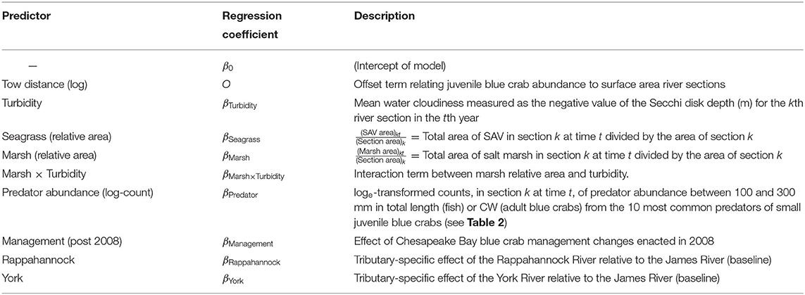
Table 1. Descriptions of predictors used in all initial models.

Seagrass

Historically, emphasis was placed on seagrass meadows as the preferred nursery for small (i.e., <30 mm CW) juvenile blue crabs (Orth and van Montfrans, 1987; Perkins-Visser et al., 1996; Hovel and Lipcius, 2002; Ralph et al., 2013) due to the high densities of juvenile crabs and settlement of postlarvae (Olmi III et al., 1990; Welch et al., 1997; van Montfrans et al., 2003) in seagrass meadows over alternative structured and unstructured substrates (Orth and van Montfrans, 1987; Lipcius et al., 2005). Effects of seagrass area are likely influenced by the spatial extent of the river section. Thus, we defined a relative seagrass area metric by dividing the area of seagrass cover within each river section in each year by the area of that section to yield a relative seagrass area metric (i.e., percent area covered, PAC). Hereafter, we refer to the spatiotemporal unit representing a given river section in each year as a section-year.

Marsh

Salt marshes may serve as nursery habitat for juvenile blue crabs, particularly in locations where seagrass is absent or declining (Jivoff and Able, 2003; Bishop et al., 2010; Johnson and Eggleston, 2010). In the Gulf of Mexico, juvenile blue crab abundance is high in both seagrass and salt marsh habitats (Thomas et al., 1990; Rozas and Minello, 1998; Heck et al., 2001). In tethering experiments, survival is often comparable between the two habitats, both of which exhibit higher survival relative to unstructured habitat (e.g., Minello et al., 2003). Similar to seagrass, we defined a relative marsh area metric for each section-year.

Turbidity

Strong turbidity gradients exist in each tributary (Nichols and Thompson, 1973; Kuo et al., 1978; Lin and Kuo, 2003; Filippino et al., 2017). Dissolved and particulate suspended solids are imported from surrounding watersheds to tributaries via terrestrial runoff. In contrast, seawater from estuarine mouths is relatively clear. Divergence in turbidity is apparent when comparing marine (i.e., polyhaline) to mesohaline and oligohaline, highly turbid upriver areas, where water clarity is frequently driven by allochthonous inputs and sediments from the surrounding watershed. The estuarine turbidity maximum (ETM), a region of elevated suspended solid concentrations and reduced light availability, occurs near the limit of salt intrusion in each tributary, where turbidity peaks (Sanford et al., 2001).

Turbidity may provide juvenile blue crabs with protection from visual predators (Cyrus and Blaber, 1987; Marley et al., 2020) and from cannibalism by larger congeners (O'Brien et al., 1976) through a reduction in light intensity. Upriver unstructured habitat is turbid, whereas similar habitat downriver has lower turbidity, such that upriver unstructured habitat can also serve as an effective nursery (Lipcius et al., 2005; Seitz et al., 2005). Hence, mean turbidity per section-year was included as a continuous covariate.

Marsh-Turbidity Interaction

Whereas seagrass meadows do not occur in high-turbidity areas due to light requirements, extensive salt marshes are present in both high- and low-turbidity regions of the tributaries. As such, turbidity may modify the effectiveness of structured salt marsh habitat as nursery for juvenile crabs by decreasing predatory foraging efficiency through both low visibility (turbidity) and structural impediments (marsh grass) (Ajemian et al., 2015). For this reason, the interaction between marsh area and turbidity was included in the analysis. We recognize that there may be confounding variables with turbidity, such as location along the upriver-downriver gradient and resources such as prey availability. Hence, our interpretations will be limited to a association between crab abundance and turbidity.

Predation

Although physical refuges can reduce predator foraging success, predator density may also determine survival (Mintz et al., 1994). For example, high abundances of juvenile blue crabs in low salinity regions have been linked to low predator abundance in those regions (Posey et al., 2005). Predators for each section-year were determined from the literature and abundances of the 10 most important predators of small juvenile blue crabs, including larger conspecifics (Table 2), were obtained from the Virginia Institute of Marine Science Juvenile Fish and Blue Crab Trawl Survey (hereafter VIMS Trawl Survey) (Tuckey and Fabrizio, 2020). Predator densities were estimated for individuals between 100 and 300 mm in total fish length (or CW for blue crabs), with the lower bound defining the smallest size able to capture and consume small juvenile blue crabs (Scharf et al., 2000), and the upper bound representing animals which would be expected to consume smaller juvenile blue crabs.

TABLE 2

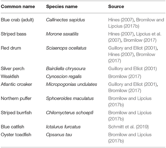
Table 2. List of predator species considered in predation abundance variable.

Tributary

The three tributaries in our study vary in geography, morphology, and hydrology. Average discharge is relatively high in the James River (194 m³ s⁻¹) and lower in the Rappahannock and York Rivers (47 m³ s⁻¹ and 31 m³ s⁻¹, respectively) (Cronin, 1971). Additionally, the three tributaries are positioned along a latitudinal gradient in Chesapeake Bay, with the Rappahannock River being northernmost, the James River southernmost and closest to the Bay mouth, and the York River intermediate. Finally, these tributaries vary substantially in surface area (Cronin, 1971). The James River is the largest at 513.0 km², the York River is the smallest at 162.5 km², and the Rappahannock River is intermediate at 307.5 km² (Smock et al., 2005). Variation in these physical characteristics may affect blue crab abundance and thus, tributary was considered as a predictor in the model.

Management

Early in the 1990s the blue crab spawning stock in Chesapeake Bay declined by 80% (Lipcius and Stockhausen, 2002), and average annual female abundance dropped 50% from 172 million crabs in 1989–1993 to 86 million crabs in 1994–2007 (MDNR, 2019). As a consequence, larval abundance and postlarval recruitment were lower by approximately 1 order of magnitude (Lipcius and Stockhausen, 2002). The sharp decline resulted in a range of management and recovery actions implemented from 2001 through 2008, including establishment of an extensive spawning sanctuary that encompassed about 75% of the spawning grounds in Chesapeake Bay (Lipcius et al., 2001, 2003; Lambert et al., 2006). Most notably, severe fishery reductions were implemented in 2008 by the three management agencies, which included the Virginia Marine Resources Commission, Potomac River Fisheries Commission, and Maryland Department of Natural Resources (MDNR), leading to a 34% reduction in female landings across Maryland and Virginia (MDNR, 2019) and triggering population recovery in subsequent years. Since 2008, annual female abundance rebounded to pre-1994 levels, and stabilized at an average of 161 million crabs during 2008–2019 (MDNR, 2019). We included management status (before and after 2008, with 2009 being the first recruitment period after management change) as a categorical predictor to capture potential effects on juvenile blue crab abundance due to increases in female blue crab abundance in response to regulatory changes that were implemented in 2008. However, we also realize that the effects of management may be interactive with those of other factors (e.g., management may increase abundance in marsh habitats but not in unvegetated areas), and thus we interpret the results for the additive effect of management with caution; also see Appendix 1.

Sampling and Data Processing

Juvenile blue crab and predator abundance data were obtained from the fisheries-independent VIMS Trawl Survey (Tuckey and Fabrizio, 2020). Beginning in March 1996 and continuing to the present, stratified-random and fixed-site sampling has been conducted monthly in the James, York, and Rappahannock Rivers using consistent gear, research vessel, and methodology. Secchi disk measurements, a proxy for turbidity, are collected immediately following each trawl tow. This sampling design provided a monthly time series of juvenile blue crab and predator catch data as well as water quality data (temperature, turbidity) in each tributary. The maximum size of predators (300 mm fish total length or crab carapace width) represent the sizes that are reliably captured by the VIMS Trawl Survey (Tuckey and Fabrizio, 2020).

GIS data on submersed aquatic vegetation (SAV) and salt marsh distributions were used as explanatory habitat variables. SAV polygons digitized from annual aerial photographs were obtained from the VIMS SAV program, while polygons of salt marsh distributions were obtained from the Shoreline and Tidal Marsh Inventory dataset from the VIMS Center for Coastal Resource Management.

The spatiotemporally varying samples from the VIMS Trawl Survey were aggregated to annually indexed areal units for the period 1996 to 2017. We limited the months considered for each year to April–December to avoid bias in crab distributions associated with winter dormancy (Hines, 2007). First, each tributary was divided along its axis into sections approximately five km in length resulting in K = K₁+K₂+K₃ = 37 total areal units, or sections (K₁ = 14 for James, K₂ = 13 for Rappahannock, and K₃ = 10 for York), which excluded one polygon at the mouth of the James representing the first five km because no samples were collected in this region by the trawl survey (Figure 1). Areal unit definitions are discussed in Appendix 2. For each kth areal unit within each tth year (i.e., (k, t)th section-year), blue crab catch and tow distance (m) information were summed to derive values of total abundance and total tow distance. Secchi disk depth and log_e-transformed predator abundance values were averaged within each (k, t). Finally, marsh and seagrass area within each section-year divided by the total area of each section were used as a relative habitat area metric for each structurally complex habitat. The aggregated trawl data resulted in 814 section-year observations. All but one of the 814 section-years contained trawl tows, and the exception was from 2017. This aggregation resulted in values of relevant response and predictor variables for each river section k in each year t.

Model Development and Specification

The spatiotemporal structure of the data in this study required complex modeling because sampling sites did not represent independent replicates. The study region covered three tributaries, each comprised of a set of k = 1, ..., K_g non-overlapping areal units (sections), g = 1, 2, 3, and data were recorded for each section for t = 1, ..., T consecutive time periods (T = 21 years over 1996–2016, due to the 2017 data being withheld for out-of-sample cross validation; see Model Implementation and Validation below). A multilevel (hierarchical) spatiotemporal Bayesian model framework for discrete responses (count data) was used to evaluate the effects of predictors while simultaneously accounting for spatiotemporal dependence. We used temporal extensions of conditional autoregressive (CAR) models (Waller et al., 1997) to examine spatiotemporal patterns in the abundance of juvenile blue crabs among potential nursery areas. To determine the necessary model complexity to capture spatial and temporal patterns in juvenile blue crab abundance, we constructed five model variants with various spatiotemporal dependence structures. Specifically, we compared models that (i) ignored spatial and temporal autocorrelation, (ii) considered exclusively spatial autocorrelation, (iii) considered separable (i.e., non-interacting) spatial and temporal autocorrelation (split into (3a) and (3b)), and (iv) considered fully non-separable (i.e., interacting) spatiotemporal autocorrelation.

Model 1

The simplest model considered in this study was a Poisson generalized linear mixed-effects model with a random effect for all river sections k = 1, ..., K:

$\begin{array}{l}{Y}_{kt}|{\mu }_{kt}~\text{Pois}({\mu }_{kt})\\ \ln ({\mu }_{kt})=\underset{p}{\overset{i=0}{{{\displaystyle \sum }}^{\text{}}}}{x}_{kti}{\beta }_i+O_{kt}+{\theta }_k\\ {\theta }_k|{\sigma }_{\theta }^2~N(0,{\sigma }_{\theta }^2)\\ {\beta }_i~N(0,100)\\ {\sigma }_{\theta }^2~\text{inverse-Gamma}(1,1)& (1)\end{array}$

The response data, juvenile crab counts, are denoted by Y_kt, for the kth section in year t. Tow distances, known offsets that have been log-transformed, are denoted by O_kt. An offset variable is one that is treated like a regression covariate whose slope parameter is fixed at 1. Offset variables are most often used to scale the modeling of the mean structure when the response variable is expected to be proportional to the offset term. A vector of predictors (see Table 1), x_kt = (1, x_kt1, ..., x_ktp) is denoted for each (k, t), and includes x_kt0 = 1 which corresponds to the intercept term. Model 1 included an independent and identically distributed (i.i.d.) random effect, θ_k. This parameter was normally distributed and accounted for section-specific variation only and did not consider spatial autocorrelation among neighboring sections or temporal autocorrelation within a given section through time. All fixed-effect regression coefficients were given a normal prior distribution with mean 0 and variance 100. The random-effect variance ${\sigma }_{\theta }^2$ was given an inverse-Gamma(1, 1) hyperprior, which is reasonably diffuse to reflect the lack of information about the parameter.

Model 2

This model considered the effects of spatial autocorrelation among neighboring river sections through the substitution of i.i.d. θ_k with conditionally autoregressive (CAR) Φ_k (Ver Hoef et al., 2018):

$\begin{array}{ll}\begin{array}{l}{Y}_{kt}|{\mu }_{kt}~Pois({\mu }_{kt})\hfill \\ \ln ({\mu }_{kt})={\displaystyle \sum }_{i=0}^p{x}_{kti}{\beta }_i+O_{kt}+{\Phi }_k\hfill \\ \Phi |\Sigma ~MVN(0,\Sigma )\hfill \\ \Sigma ={\sigma }_{\Phi }^2{(D-\lambda W)}^{-1}\hfill \\ {\beta }_i~N(0,100)\hfill \\ \lambda ~U(0,1)\hfill \\ {\sigma }_{\Phi }^2~inverse-Gamma(1,1)\hfill \end{array}& (2)\end{array}$

where the joint probability distribution of Φ = (Φ₁, ..., Φ_K) is specified as a multivariate normal distribution with a mean vector of 0s and variance-covariance matrix Σ. The Σ matrix describes spatial correlation based on the neighborhood structure specified by a K×K adjacency matrix, W, and an autocorrelation parameter λ, which controls the degree of spatial autocorrelation among neighboring sections across the entire region of study. We employed a binary weighting scheme for W where $w_{k,k^{\prime }}=0$ for all (k, k′) unless areal units k≠k′ share a common border. The influence of neighboring sections on a given section was standardized by subtracting λW from D, a diagonal matrix where D_{k, k} is the number of neighbors for section k. This specification effectively scaled spatial dependence by the number of neighbors for each section while avoiding model unidentifiability of the intrinsic CAR (ICAR) structure (e.g., Chiu et al., 2013). The parameter λ was constrained between 0 and 1 (hence, non-negative) through a uniform prior. This spatial dependence structure was assumed to be homoscedastic through the variance parameter ${\sigma }_{\Phi }^2$, again with an inverse-Gamma(1, 1) hyperprior. The regression coefficients were given the same prior distributions as before.

Model 3

Models 3a and 3b considered separable spatial and temporal dependence (Waller et al., 1997) by expanding on Model 2 through the addition of an autoregressive temporal autocorrelation structure of order 1, i.e., AR(1), at two spatial resolutions. The model equations below for 3a and 3b hold for all k and t. Model 3a included an autocorrelated normally distributed error term η_t, with η = (η₁, ..., η_T) and a global temporal autocorrelation parameter, ρ, and variance ${\sigma }_{\eta }^2$, where ρ is given a uniform prior distribution between 0 and 1, (again, non-negative) and the remaining model parameters are given the same prior distributions as before.

$\begin{array}{ll}\begin{array}{l}{Y}_{kt}|{\mu }_{kt}~Pois({\mu }_{kt})\hfill \\ \ln ({\mu }_{kt})={\displaystyle \sum }_{i=0}^p{x}_{kti}{\beta }_i+O_{kt}+{\Phi }_k+{\eta }_t\hfill \\ \Phi |\Sigma ~MVN(0,\Sigma )\hfill \\ \Sigma ={\sigma }_{\Phi }^2{(D-\lambda W)}^{-1}\hfill \\ {\eta }_t|\rho ,{\eta }_{t-1},{\sigma }_{\eta }^2~N(\rho {\eta }_{t-1},{\sigma }_{\eta }^2)for all t=2,3,\mathrm{...},T\hfill \\ {\beta }_i~N(0,100)\hfill \\ \lambda ,\rho ~U(0,1)\hfill \\ {\sigma }_{\Phi }^2,{\sigma }_{\eta }^2~inverse-Gamma(1,1)\hfill \end{array}& (\mathrm{3a})\end{array}$

In contrast, Model 3b stipulated tributary-specific temporal autocorrelation for g = 1, 2, 3:

$\begin{array}{ll}\begin{array}{l}{Y}_{kt}|{\mu }_{ktg}~Pois({\mu }_{ktg})\hfill \\ \ln ({\mu }_{ktg})={\displaystyle \sum }_{i=0}^p{x}_{kti}{\beta }_i+O_{kt}+{\Phi }_k+{\eta }_t\hfill \\ \Phi |\Sigma ~MVN(0,\Sigma )\hfill \\ \Sigma ={\sigma }_{\Phi }^2{(D-\lambda W)}^{-1}\hfill \\ {\eta }_{gt}|{\rho }_g,{\eta }_{g,t-1},{\sigma }_{\eta }^2~N({\rho }_g{\eta }_{g,t-1},{\sigma }_{\eta }^2)for all t=2,3,\mathrm{...},T\hfill \\ logit({\rho }_g)=logit(P)+r_g\hfill \\ r_3=-r_1-r_2\hfill \\ {\beta }_i~N(0,100)\hfill \\ \lambda ,\rho ~U(0,1)\hfill \\ {\sigma }_{\Phi }^2,{\sigma }_{\eta }^2~inverse-Gamma(1,1)\hfill \\ r_1,r_2~N(0,0.25)\hfill \end{array}& (\mathrm{3b})\end{array}$

Here, η_gt is the normally distributed AR(1) error term for year t and tributary g, with a local temporal autocorrelation parameter ρ_g and global variance ${\sigma }_{\eta }^2$. the complete set is denoted by η = (η₁, η₂, η₃), where η_g = (η_g1, η_g2, ..., η_gT). Here, each ρ_g on the logit scale is modeled as the logit of a global temporal autocorrelation parameter P plus a tributary-specific offset r_g, subject to the sum-to-zero constraint $\sum _{i=1}^3{r}_g=0$. Two of the r_gs are given normal priors of N(0, 0.25) which reflect a compromise between the lack of pre-existing knowledge about these parameters and a desire to constrain the distributions from unrealistic extremes (Gelman et al., 2013, and Supplementary Figure 1). The inverse-logit transformation, ${\mathrm{\text{logit}}}^{-1}(u)=\frac{e^u}{1+e^u}$ for any real number u (here, u = logit(ρ_g)), constrains ρ_g between 0 and 1. Similarly, P is given a uniform prior between 0 and 1. The remaining model parameters were given the same prior distributions as before.

Model 4

For the final model, we considered a non-separable spatiotemporal random effect. The spatiotemporal structure includes a multivariate first-order autoregressive process with a first-order spatial CAR structure. The data level and linear predictor of the resulting hierarchical model are:

$\begin{array}{cccc}{Y}_{kt}|{\mu }_{kt}& ~\text{Pois}({\mu }_{kt})& \text{and}& \ln ({\mu }_{kt})=\underset{i=0}{\overset{P}{{{\displaystyle \sum }}^{\text{}}}}{x}_{kti}{\beta }_i+O_{kt}+{\Phi }_{kt}.\end{array}$

Here, the Φ_kt term is the random effect associated with section k in year t, with the complete set denoted by Φ = (Φ₁, ..., Φ_T), where each Φ_t = (Φ_1t, ..., Φ_Kt) is the tth map of spatial random effects.

$\begin{array}{ll}\begin{array}{l}\Phi |\Sigma ~MVN(0,\Sigma )\hfill \\ \Sigma ={\sigma }_{\Phi }^2{(D-\lambda W)}^{-1}\hfill \\ {\Phi }_t|\rho ,{\Phi }_{t-1},\Sigma ~MVN(\rho {\Phi }_{t-1},\Sigma ),whent>1\hfill \\ \Sigma ={\sigma }_{\Phi }^2{(D-\lambda W)}^{-1}\hfill \\ {\beta }_i~N(0,100)\hfill \\ {\sigma }_{\Phi }^2,{\sigma }_{\eta }^2~inverse-Gamma(1,1)\hfill \\ \lambda ,\rho ~U(0,1).\hfill \end{array}& (4)\end{array}$

The spatiotemporal autocorrelation structure is stipulated by replacing η_t in Model 3a with the entire Φ_t map, an approach employed by Rushworth et al. (2014), and represents the spatiotemporal pattern in the mean response with a single set of spatially and temporally autocorrelated random effects. The Φ_t map follows a multivariate autoregressive process of order one. Thus, in year t = 1, the Φ₁ map assumes a strictly CAR structure. However, when t>1, temporal autocorrelation is induced by explicitly allowing Φ_t to have conditional mean equal to ρΦ_t−1.

The regression coefficients, autocorrelation parameters, and variance parameters were given the same prior distributions as in previous models.

Model Implementation and Validation

For each model, Bayesian inference required numerical approximation of the joint posterior distribution of all model parameters including the vectors of random effects θ, Φ, and η. To this end, we implemented the above models using the Stan programming language for Bayesian inference to generate Markov chain Monte Carlo (MCMC) samples from the posterior (Gelman et al., 2015). For each model, we ran four parallel Markov chains, each with 15,000 iterations for the warm-up/adaptive phase (and subsequently discarded as burn-in), and another 15,000 iterations as posterior samples (i.e., 60,000 draws in total for posterior inference). Convergence of the chains was determined both by visual inspection of trace plots (e.g., Supplementary Figure 2) and through inspection of the split $\widehat{R}$ statistic. All sampled parameters had an $\widehat{R}$ value less than 1.01, indicating chain convergence (Gelman et al., 2015). Covariates and interactions whose regression coefficients had Bayesian confidence intervals (CIs) that excluded 0 at a confidence level of 80% were considered scientifically relevant to juvenile blue crab abundance (see Appendix 3). All CIs referenced here are highest posterior density intervals (HPDIs) (McElreath, 2018).

Model validation and relative predictive performance were assessed using out-of-sample cross validation (CV), whereby a subset of the full data was used to train models, and the trained models were then used to predict the withheld data. Given the spatiotemporal dependence structures within our model, common CV procedures, such as leave-one-out (LOO), are difficult to interpret if the goal is to assess predictive performance, because withheld observations depend on other observations from different time periods and different spatial units in addition to the dependence on the model parameters (Bürkner et al., 2021). For example, withholding random observations in time-series models will still allow information from the future to influence predictions of the past. Instead, we employed the leave-future-out (LFO) CV approach to evaluate predictive performance through withholding future samples (Bürkner et al., 2020). Thus, prior to CV analysis, the data from the final year of the study, 2017, were excluded from the models. Then, the above Models 1–4 were fitted to the reduced dataset for both model inference (whose results appear under Results) as well as CV. For CV, 80% Bayesian prediction intervals were computed from the posterior predictive distributions of the excluded values, as a forecasting exercise. The final step of CV analysis was to compare the excluded blue crab count values to the forecast prediction intervals. Note that due to missing data in one of the sections in 2017 (see Data Summary below), CV was only possible for n = 36 sections.

Prioritized Areas for Conservation

Using posterior distributions derived from Model 4 (justified under Results), we aggregated over time and made spatial-only predictions of juvenile blue crab abundance to identify areas of high abundance. For continuous predictors, data were aggregated for each section over 2009–2017 to obtain inter-annual grand means, i.e., ${\overline{x}}_{k+i}=\sum _{t=1}^T{x}_{kti}/T$ for continuous predictor variable x_kti, where T = 9 for all sections except T = 8 for the section with no trawl data in 2017. The same aggregation was applied respectively to the log-transformed tow distance offset term O_kt and each dth posterior draw for the spatiotemporal random-effect term ${\Phi }_{kt}^{(d)}$ to define ${\overline{O}}_{k+}$ and ${\overline{\Phi }}_{k+}^{(d)}$. Thus, for abundance, ${\overline{\mu }}_{k+}^{(d)}$ denotes a temporally aggregated posterior draw of the expected abundance from replacing μ_kt of Model 4 with ${\overline{\mu }}_{k+}^{(d)}$ that was computed using ${\overline{x}}_{k+i},{\overline{O}}_{k+}$, and ${\overline{\Phi }}_{k+}^{(d)}$; the set $\left\{{\overline{\mu }}_{k+}^{(1)},{\overline{\mu }}_{k+}^{(2)},...{\overline{\mu }}_{k+}^{(60000)}\right\}$ for each k forms a pseudo-posterior distribution of the temporally aggregated expected abundance ${\overline{\mu }}_{k+}$ for spatial section k. (A true posterior distribution would require fitting a spatial-only version of Model 4 that directly models temporally averaged counts ${\overline{y}}_{k+}$.) We limited spatial-only comparisons to 2009–2017 due to the change in management following 2008, which was a categorical predictor and could not be reasonably averaged over time. In addition to inspecting the n = 37 values of pseudo-posterior median for ${\overline{\mu }}_{k+}$ (k = 1, ..., n), we computed tributary-specific standardized values (centered and scaled to have unit variance) of the pseudo-posterior medians of ${\overline{\mu }}_{k+}$ to determine regions of locally high and low abundance relative to each tributary. Resulting sections with predictions corresponding to higher average relative juvenile blue crab abundance were interpreted as more productive within tributary, whereas sections with predictions corresponding to lower average relative juvenile blue crab abundance were interpreted as less productive within tributary.

Results

Model Selection and Validation

Cross validation indicated that the non-separable spatiotemporal model, Model 4, best described patterns in juvenile blue crab abundance. The 80% posterior prediction intervals from Model 4 contained 81.1% of withheld 2017 data, while Models 1 (random effect only), 2 (spatial-only CAR model), 3a (spatial CAR model with separable, global AR(1) term), and 3b (spatial CAR model with separable, tributary-specific AR(1) term) captured 21.6, 18.9, 43.2, and 70.3% of withheld data, respectively (Figure 2). A full description of model validation and predictive performance is provided in Appendix 3. Hereafter, inferences are made from Model 4 only.

FIGURE 2

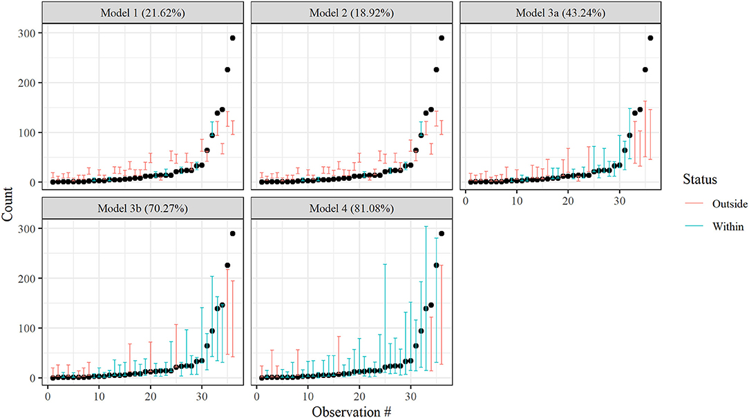
Figure 2. Leave-future-out cross validation results for Models 1–4. Bars denote nominal 80% Bayesian prediction intervals derived from posterior predictive distributions, while dots depict observed crab counts for 2017. Red bars indicate an observed value is outside the prediction interval, while blue bars indicate an observed value is within the prediction interval. Actual coverage percentages of prediction intervals (= % of blue) appear in the panel headings.

Data Summary

In total, 75,103 juvenile blue crabs between 20–40 mm CW were captured between 1996 and 2017 from April to December in the York, James, and Rappahannock Rivers. The highest abundances of juvenile blue crabs occurred in upriver locations of each tributary (Figures 3a, 4a). Relative seagrass area was highest in the York River and lowest in the James River (Table 3). Relative marsh area and turbidity were highest in the York River and lowest in the Rappahannock River (Table 3). Within each tributary, turbidity generally increased with distance upriver.

FIGURE 3

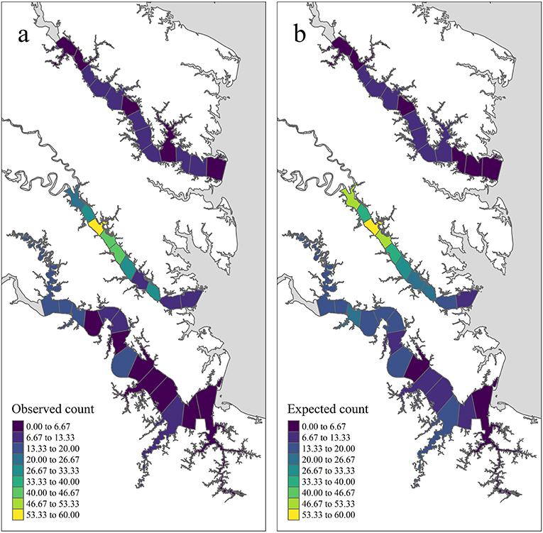
Figure 3. Temporally aggregated observed and expected juvenile blue crab abundance in each tributary section based on inter-annual grand means of model quantities from years 2009–2017 and management after 2008 (see the Methods: Prioritized Areas for Conservation Section for definitions) (a) shows the mean observed juvenile blue crab abundance (${\overline{y}}_{k+}$), while (b) shows the pseudo-posterior median of the expected abundance on the count scale (${\overline{\mu }}_{k+}$).

FIGURE 4

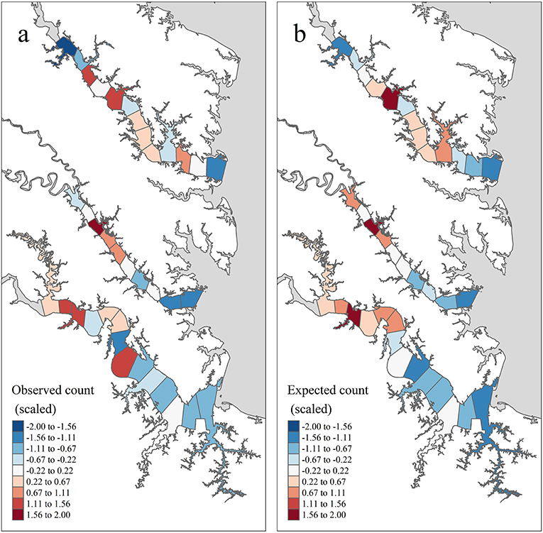
Figure 4. Temporally aggregated observed and expected juvenile blue crab abundance in each tributary section based on inter-annual grand means of model quantities from years 2009–2017 and management after 2008 (see the Methods: Prioritized Areas for Conservation Section for definitions), standardized within tributary. (a) shows the tributary-specific standardized value of ${\overline{y}}_{k+}$ (mean observed juvenile blue crab abundance), while (b) shows the tributary-specific standardized value of ${\overline{\mu }}_{k+}$ (pseudo-posterior median of the expected abundance on the count scale).

TABLE 3

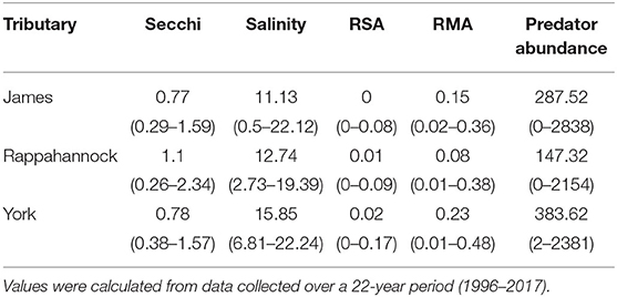
Table 3. Mean (minimum–maximum) section-year values for Secchi disk depth, salinity, relative seagrass area (RSA), relative marsh area (RMA), and predator abundance for each tributary.

Drivers of Juvenile Blue Crab Abundance

Based on posterior distributions of Model 4 parameters, tributary, turbidity, relative marsh area, and relative marsh area × turbidity were relevant drivers of juvenile blue crab abundance. All tributaries differed in average juvenile blue crab abundances, with posterior probabilities P(β_York>β_James|data)>0.99, P(β_York>β_Rappahannock|data)>0.99, and P(β_James>β_Rappahannock|data) = 0.99. Turbidity, marsh, and their interaction positively influenced juvenile blue crab abundance — posterior medians (and 80% Bayesian CIs) were: β_Turbidity = 0.48 (0.20–0.77), β_Marsh = 2.55 (1.07–4.01), and β_{Marsh x Turbidity} = 3.42 (1.34–5.49). Regression coefficients β_Seagrass, β_Predator, and β_Management had respective 80% CIs that included 0. Supporting posterior summaries and graphics are in Table 4 and Supplementary Figure 3.

TABLE 4

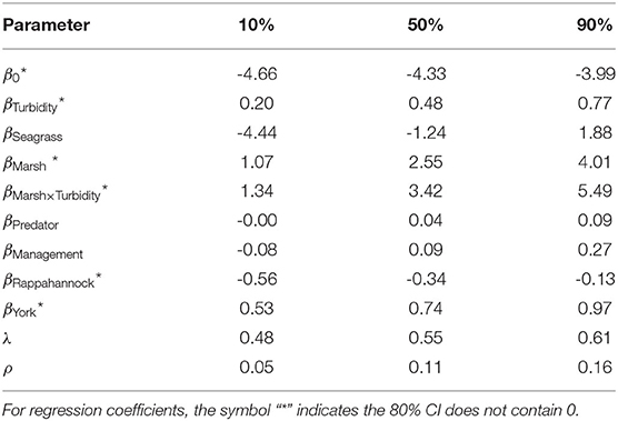
Table 4. Posterior summary statistics (median and 80% Bayesian CI's) of regression coefficients β as well as autocorrelation parameters λ (spatial) and ρ (temporal) from Model 4.

Conditional effects plots (Figures 5,6) were used to visualize the relationship between juvenile blue crab abundance and predictors relative marsh area and turbidity. For conditional effects plots, we considered the function μ_cond(x_Turbidity, x_Marsh) = x_Turbidityβ_Turbidity+x_Marshβ_Marsh+x_Marshx_Turbidityβ_{Marsh × Turbidity}+β_Management+ln(1000), which re-expresses the juvenile blue crab expected abundance μ_kt as a function of x_Turbidity and x_Marsh as the only varying predictors, while all other continuous predictor variables were held at 0 and the tow offset term was held at 1,000 m, while categorical variables were held at the James River (tributary) and post 2008 period. The relationship between each varying predictor and μ_cond was plotted (along with confidence bands) with the other varying predictor held at fixed percentiles (1, 20, 40, 60, 80, and 99%) to visualize interaction effects. Relative marsh area influenced juvenile blue crab abundance negatively at low turbidities (i.e., ≤ −0.81 = median) and positively at high turbidities (i.e., ≥−0.81 = median) (Figure 5). In contrast, turbidity influenced crab abundance positively at both low and high relative marsh area values, with the strength of the relationship between turbidity and abundance growing progressively stronger at high relative marsh area values (Figure 6).

FIGURE 5

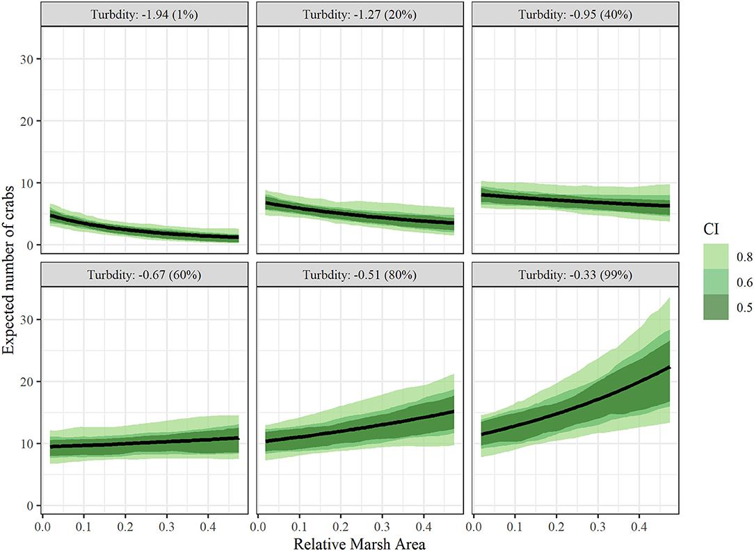
Figure 5. Conditional effects plots depicting relationship between juvenile blue crab abundance per 1000 m towed (μ_cond) vs relative marsh area (RMA) at turbidity values corresponding to 1, 20, 40, 60, 80, and 99% percentiles to visualize interaction effects between relative marsh area and turbidity on crab abundance. All other continuous variables were held at 0 and categorical variables at the James River (tributary) and post 2008 (management). Colored bands indicate Bayesian confidence bands of μ_cond. (See the Drivers of Juvenile Blue Crab Abundance Section for definitions).

FIGURE 6

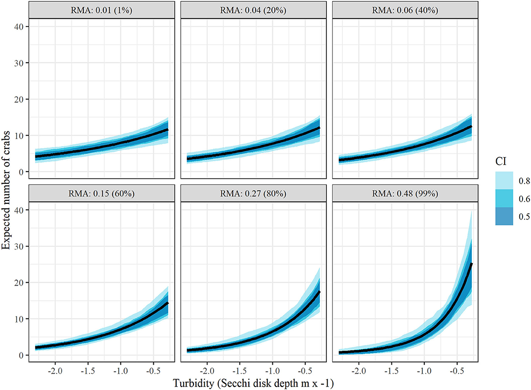
Figure 6. Conditional effects plots depicting relationship between juvenile blue crab abundance per 1000 m towed (μ_cond) vs turbidity at relative marsh area (RMA) values corresponding to 1, 20, 40, 60, 80, and 99% percentiles to visualize interaction effects between relative marsh area and turbidity on crab abundance. All other continuous variables were held at 0 and categorical variables at the James River (tributary) and post 2008 (management). Colored bands indicate Bayesian confidence bands of μ_cond. (See the Drivers of Juvenile Blue Crab Abundance Section for definitions).

Spatiotemporal Dependence

The posterior distribution of λ indicated that substantial spatial dependence existed within the data (Supplementary Figure 4). Posterior distributions of λ and ρ yielded medians (80% Bayesian CIs) of 0.61 (0.55–0.68) and 0.14 (0.08–0.19), respectively. Although the magnitude of ρ was small, this non-separable spatiotemporal model, when compared to simpler models, gave leave-future-out 80% Bayesian prediction intervals that had the highest coverage of the withheld 2017 data, and the coverage was close to its nominal 80% (Figure 2). Moreover, among the competing models the spatiotemporal structure was strong enough that posteriors of the fixed-effect coefficients changed markedly when spatially and spatiotemporally structured random effects were included (Supplementary Figure 5).

Prioritized Areas for Conservation

According to pseudo-posterior medians of ${\overline{\mu }}_{k+}$ (based on temporally aggregated predictors, model offset, and spatiotemporal random-effects), upriver sections of tributaries consistently harbored highest crab abundances (Figures 3b, 4b). In particular, upriver sections in the York River were very high, with a pseudo-posterior median of 30–60 crabs per 1,000 m towed. Upriver sections in the James River had a pseudo-posterior median of 13–26 crabs per 1,000 m towed, whereas those in the Rappahannock River were much lower at 0–13 crabs per 1,000 m towed. Pseudo-posterior medians for ${\overline{\mu }}_{k+}$ were generally consistent with observed juvenile blue crab abundances ${\overline{y}}_{k+}$ in each section from 2009–2017 (Figures 3, 4).

Discussion

Abundance of juvenile blue crabs varied spatially both within and among the three tributaries, James, York and Rappahannock Rivers. Within all tributaries, abundance of juvenile blue crabs consistently peaked in upriver sections. Given the limited mobility of juvenile blue crabs <60 mm CW, we interpret high 20–40 mm CW abundance in upriver areas as reflective of highly productive nursery habitats, as previously hypothesized for the York River (Lipcius et al., 2005; Seitz et al., 2005). Moreover, juvenile blue crab abundance was associated with specific environmental characteristics, especially with high turbidity and extensive marsh area near the turbidity maximum of each tributary. These findings offer an initial quantification of multiple environmental components of highly productive nursery locations within the seascape paradigm for juvenile blue crabs in lower Chesapeake Bay.

Environmental Determinants of Juvenile Blue Crab Abundance

Availability of marsh habitat and high turbidity were the most important predictors of juvenile blue crab abundance, which was strongly and positively related to turbidity, and increased with the availability of salt marsh habitat relative to geographic area. However, the substantial interaction between marsh habitat and turbidity required that inferences on the relationship between marsh habitat or turbidity and juvenile blue crab abundance be made within the context of the other factor.

In areas characterized by low turbidity (i.e., mean Secchi depth >1 m), the effect of marsh habitat ranged from negligible to negative. Conversely, in locations of high turbidity (i.e., mean Secchi depth <1 m), juvenile blue crab abundance was positively associated with availability of marsh habitat. About half of the section-years considered in our study were characterized by high turbidity where marsh availability was positively related to crab abundance. Turbidity and crab abundance were always related positively, and this relationship grew stronger (steeper slope) as marsh area increased in a river section.

While relative area of adjacent marsh habitat was positively related to juvenile blue crab abundance, other potential nursery habitats were weakly associated with crab abundance. At the tributary spatial scale, the areal extent of marsh habitat relative to the area of river sections was much greater than that of seagrass meadows, particularly in the York and James Rivers. Moreover, section-years harboring seagrass meadows (such as in downriver York and midriver-downriver Rappahannock sections) were not associated with high juvenile blue crab abundance. This was particularly surprising for seagrass, which has long been considered the preferred nursery habitat for small juvenile blue crabs (Orth and van Montfrans, 1987; Lipcius et al., 2007). The lack of association between juvenile blue crab abundance and seagrass habitats may reflect differences between nursery habitat contributions per unit area (proposed by Beck et al., 2001) versus effective nursery habitat and total contribution to the adult segment of the population (proposed by Dahlgren et al., 2006). The potentially high production of juvenile blue crabs per unit area expected in river sections with seagrass meadows may have been obfuscated by the abundance of juvenile blue crabs observed throughout the broad areal extent of salt marsh habitat. The magnitude of a seagrass effect may also have been biased by the seascape surrounding seagrass beds. Trawling next to seagrass beds may be biased because some fraction of juvenile crabs <40 mm CW remain within the seagrass beds (Orth and van Montfrans, 1987; Lipcius et al., 2005; Seitz et al., 2005; Ralph et al., 2013), and adjacent salt marshes (Thomas et al., 1990; Rozas and Minello, 1998; Minello et al., 2003, 2012), where they are not susceptible to trawl gear. In addition, juveniles emigrating from downriver seagrass beds may move not just to the trawl area downriver, but also to unstructured habitats outside the tributaries, which was not considered in our study. Given that we don't know the fractions of 30–40 mm CW juveniles that remain in seagrass beds or salt marshes, and that some juveniles may be emigrating away from trawl sites adjacent to seagrass and salt marsh habitats, we focus our conclusions to emphasize the nursery value of salt marshes as an alternative critical nursery habitat.

Predator abundance was not related to juvenile blue crab abundance. The apparent lack of an effect of predator abundance on juvenile blue crab abundance may reflect high refuge capacity of crab nurseries or increased availability of alternative prey in locations harboring high blue crab abundance (Lipcius et al., 2005). Moreover, finish predators are highly mobile and not likely to remain in a specific section. These findings suggest that abundance of juvenile blue crabs at the regional scale is largely driven by bottom-up controls rather than top-down controls, which is consistent with studies of blue crab abundance in highly turbid, upriver localities harboring expansive marsh habitat (Seitz et al., 2003, 2005; Posey et al., 2005). Alternatively, the strong positive relationship between juvenile blue crab abundance and turbidity may reflect the effect of turbidity on predator efficiency, as highly turbid water can reduce capture rates of both visually and non-visually oriented aquatic predators (Ortega et al., 2020). Hence, reductions in predator efficiency associated with increasing turbidity may moderate effects of predator abundance. Further investigation is warranted to understand concomitant effects of predator abundance and turbidity with respect to juvenile blue crab spatial distributions.

Finally, juvenile blue crab abundance differed substantially among the three tributaries. These spatial patterns in abundance likely reflected tributary-specific characteristics that we did not consider in our models (e.g., differences in flow, bathymetry, total area, geographic position relative to the mouth of the Chesapeake Bay, or land-use patterns). Ultimately, spatial variation in juvenile blue crab abundance among tributaries indicates that tributaries in the Chesapeake Bay are not equal as nursery areas for the blue crab population, and that further studies should quantify tributary-specific production to the population.

Effect of Management

Changes in management of the blue crab population in the Chesapeake Bay after 2009 were positively associated with juvenile blue crab abundance, but not strongly, in contrast to the findings of other studies (MDNR, 2019; Lipcius, 2020). One explanation for this result is the potential effect of cannibalism by larger juveniles and adults on small juveniles, which might negate positive effects of increased recruitment from a larger spawning stock (Lipcius and Stockhausen, 2002). More likely, the effect of management may depend upon specific habitats and seasons, especially those where Age-0 juveniles are abundant, such as during the late-summer through early-fall recruitment period and in habitats with expansive marshes. Other sections where juveniles are not as abundant, such as unvegetated habitat, may not support high levels of recruitment, which would confound a singular interpretation of management. Targeted analyses of the effects of management in specific habitats and seasons are ongoing to resolve this issue.

Prioritized Areas for Conservation

An objective of this study was to assist management to prioritize and direct restoration and conservation efforts of the blue crab within Chesapeake Bay as well as other blue crab stocks along its geographic range. Although previous focus of blue crab nursery studies was on seagrass meadows (Ralph, 2014), salt marshes and certain unstructured, high turbidity habitats appear valuable at the tributary and regional scales due to their extensive areal cover. Our best fitting model indicated that expansive salt marshes in highly turbid upriver locations are highly productive nurseries for this ecologically and economically exploited species. As a result, a major recommendation of this article is the inclusion of salt marsh habitats as conservation targets.

Relevance

The EFH provisions of the Magnuson-Stevens Act directs fishery management councils to utilize the best available science to describe and identify EFH for federally managed species and protect them to the extent practicable (MSA, 2007). The highest level of EFH information is level 4: production rates by habitat type; yet level 4 EFH information is largely unavailable for most commercially harvested species, particularly at spatial and temporal scales needed for effective fisheries management. This lack of level 4 EFH information is currently limiting the inclusion of habitat effects in stock assessments and in ecosystem-based fisheries management plans (Grüss et al., 2017). Furthermore, area-based estimates of nursery habitat value may inform decision-making related to protected area management and habitat restoration, by allowing the per unit area contribution of protected or restored habitat to be quantified (zu Ermgassen et al., 2021).

Understanding the relative contribution of structured habitats and other environmental factors on the productivity of a given area is important, as many conditions resulting in such productivity are diminishing. Some structured nursery habitats are declining, especially eelgrass Z. marina beds due to direct and indirect anthropogenic influences such as land-use change and long-term warming of Chesapeake Bay (Orth et al., 2010; Moore et al., 2014; Patrick et al., 2018). Similarly, salt marshes have been reduced by coastal development and shoreline hardening (Silliman et al., 2009).

Scientists and managers have generally assumed that when structured habitats are degraded, the services they provide such as nursery habitat for valuable marine species are lost (Peterson and Lipcius, 2003). Therefore, state and federal agencies have long invested in coastal habitat conservation and restoration to recover lost production. However, these investments have often preceded the availability of, and thus would be enhanced by the development of, rigorous analytical tools capable of quantifying the ecosystem services expected from conservation actions and habitat restoration efforts. While standalone small-scale studies have been and remain important tools to initially assess nursery value of structured habitats and other environmental factors, targeted comprehensive applications of survey data collected over broad spatial and temporal scales are a vital complement to generalize inference of nursery function, highlight highly productive regions, and inform regional management strategies.

Future Research

We assessed relative secondary production associated with spatially explicit regions, which was then related to local environmental variation. This strategy is broadly useful for assessing potential nursery capacity of specific regions, as it captures juveniles emigrating from nursery habitats to unstructured adult habitats (Beck et al., 2001). However, this method may miss other potentially important aspects of the ecology of nursery habitats operating at smaller temporal scales, such as when habitats may promote rapid growth and enhanced recruitment. As small-scale studies are uniquely suited for capturing these processes, further work is required to more precisely ascertain the contributions of these habitats and environmental variables at both large and small spatial scales.

Data Availability Statement

The data analyzed in this study is subject to the following licenses/restrictions: Data analyzed here from the Virginia Institute of Marine Science Juvenile Fish and Blue Crab Trawl Survey is available upon request pending approval by MF. Requests to access these datasets should be directed to mfabrizio@vims.edu.

Author Contributions

AH, GC, MF, and RL designed research and wrote the paper. AH and GC developed models, designed model validation, analyzed implementation, and validation results. AH processed data and conducted model implementation and validation. MF and RL advised on experimental design and model refinement.

Funding

This work was supported by AH was funded by a Willard A. Van Engel Fellowship of the Virginia Institute of Marine Science, William & Mary.

Conflict of Interest

The authors declare that the research was conducted in the absence of any commercial or financial relationships that could be construed as a potential conflict of interest.

Publisher's Note

All claims expressed in this article are solely those of the authors and do not necessarily represent those of their affiliated organizations, or those of the publisher, the editors and the reviewers. Any product that may be evaluated in this article, or claim that may be made by its manufacturer, is not guaranteed or endorsed by the publisher.

Acknowledgments

The authors thank the Associate Editor and two reviewers for their valuable suggestions. We also acknowledge William & Mary Research Computing for providing computational resources and technical support that have contributed to the results reported within this article. URL: https://www.wm.edu/it/rc. AH also thanks D Eggleston and C Patrick for their ideas as members of AH's Ph.D. Committee. This project would not have been possible without the help of J Buchanan, A Comer, W Lowery, K Nickerson, D Royster, and the many other individuals who collected blue crabs between 1996 and 2017 from the VIMS Juvenile Fish Trawl Survey; in particular, we thank W Lowery and T Tuckey for providing access to survey records.

Supplementary Material

The Supplementary Material for this article can be found online at: https://www.frontiersin.org/articles/10.3389/fmars.2022.834990/full#supplementary-material

References

Ajemian, M., Sohel, S., and Mattila, J. (2015). Effects of turbidity and habitat complexity on antipredator behavior of three-spined sticklebacks (gasterosteus aculeatus). Environ. Biol. Fishes 98, 45–55. doi: 10.1007/s10641-014-0235-x

CrossRef Full Text | Google Scholar

Beck, M. W., Heck, K. L., Able, K. W., Childers, D. L., Eggleston, D. B., Gillanders, B. M., et al. (2001). The identification, conservation, and management of estuarine and marine nurseries for fish and invertebrates: a better understanding of the habitats that serve as nurseries for marine species and the factors that create site-specific variability in nursery quality will improve conservation and management of these areas. Bioscience 51, 633–641. doi: 10.1641/0006-3568(2001)051[0633:TICAMO]2.0.CO;2

CrossRef Full Text | Google Scholar

Bishop, T. D., Miller, H. L., Walker, R. L., Hurley, D. H., Menken, T., and Tilburg, C. E. (2010). Blue crab (Callinectes sapidus Rathbun, 1896) settlement at three Georgia (USA) estuarine sites. Estuaries Coasts 33, 688–698. doi: 10.1007/s12237-020-00867-1

PubMed Abstract | CrossRef Full Text | Google Scholar

Boudreau, S. A., Shackell, N. L., Carson, S., and den Heyer, C. E. (2017). Connectivity, persistence, and loss of high abundance areas of a recovering marine fish population in the northwest atlantic ocean. Ecol. Evol. 7, 9739–9749. doi: 10.1002/ece3.3495

PubMed Abstract | CrossRef Full Text | Google Scholar

Bromilow, A. M. (2017). Juvenile Blue Crab Survival in Nursery Habitats: Predator Identification and Predation Impacts in Chesapeake Bay (Ph.D. thesis). Virginia Institute of Marine Science, William & Mary, Gloucester Point, VA.

Google Scholar

Bromilow, A. M., and Lipcius, R. N. (2017a). Mechanisms governing ontogenetic habitat shifts: role of trade-offs, predation, and cannibalism for the blue crab. Marine Ecol. Progr. Series 584, 145–159. doi: 10.3354/meps12405

CrossRef Full Text | Google Scholar

Bromilow, A. M., and Lipcius, R. N. (2017b). Mechanisms governing ontogenetic habitat shifts: role of trade-offs, predation, and cannibalism for the blue crab. Marine Ecol. Progr. Series 584, 145–159.

Google Scholar

Brown, C. J., Broadley, A., Adame, M. F., Branch, T. A., Turschwell, M. P., and Connolly, R. M. (2019). The assessment of fishery status depends on fish habitats. Fish Fisheries 20, 1–14. doi: 10.1111/faf.12318

CrossRef Full Text | Google Scholar

Bürkner, P.-C., Gabry, J., and Vehtari, A. (2020). Approximate leave-future-out cross-validation for Bayesian time series models. J. Stat. Comput. Simulat. 90, 2499–2523. doi: 10.1080/00949655.2020.1783262

PubMed Abstract | CrossRef Full Text | Google Scholar

Bürkner, P.-C., Gabry, J., and Vehtari, A. (2021). Efficient leave-one-out cross-validation for Bayesian non-factorized normal and Student-t models. Comput. Stat. 36, 1243–1261. doi: 10.1007/s00180-020-01045-4

CrossRef Full Text | Google Scholar

Camp, E. V., Lorenzen, K., and Taylor, M. D. (2020). Impacts of habitat repair on a spatially complex fishery. Estuarine Coastal Shelf Sci. 244, 106102. doi: 10.1016/j.ecss.2019.02.007

CrossRef Full Text | Google Scholar

Chiu, G., Lehmann, E., and Bowden, J. (2013). A spatial modelling approach for the blending and error characterization of remotely sensed soil moisture products. J. Environ. Stat. 4, 1–17. Available online at: http://www.jenvstat.org/v04/i09

Cronin, W. B. (1971). Volumetric, Areal, and Tidal Statistics of the Chesapeake Bay Estuary and Its Tributaries. Special Report 20, Chesapeake Bay Institute, The Johns Hopkins University, Baltimore, MD.

Google Scholar

Cyrus, D., and Blaber, S. (1987). The influence of turbidity on juvenile marine fish in the estuaries of Natal, South Africa. Continental Shelf Res. 7, 1411–1416. doi: 10.1016/0278-4343(87)90046-x

CrossRef Full Text | Google Scholar

Dahlgren, C. P., Kellison, G. T., Adams, A. J., Gillanders, B. M., Kendall, M. S., Layman, C. A., et al. (2006). Marine nurseries and effective juvenile habitats: concepts and applications. Marine Ecol. Progr. Series 312, 291–295. doi: 10.3354/meps312291

CrossRef Full Text | Google Scholar

Davis, J. L., Young-Williams, A. C., Hines, A. H., and Zmora, O. (2004). Comparing two types of internal tags in juvenile blue crabs. Fisheries Res. 67, 265–274. doi: 10.1016/j.fishres.2003.11.005

CrossRef Full Text | Google Scholar

Epifanio, C. (2007). “Biology of larvae,” in The Blue Crab, Callinectes Sapidus (College Park, MD: Maryland Sea Grant), 513–533.

Google Scholar

Epifanio, C. E. (2019). Early life history of the blue crab Callinectes sapidus: a review. J. Shellfish Res. 38, 1–22. doi: 10.2983/035.038.0101

CrossRef Full Text | Google Scholar

Etherington, L. L., and Eggleston, D. B. (2000). Large-scale blue crab recruitment: linking postlarval transport, post-settlement planktonic dispersal, and multiple nursery habitats. Marine Ecol. Progr. Series 204, 179–198. doi: 10.3354/meps204179

CrossRef Full Text | Google Scholar

Etherington, L. L., Eggleston, D. B., and Stockhausen, W. T. (2003). Partitioning loss rates of early juvenile blue crabs from seagrass habitats into mortality and emigration. Bull. Marine Sci. 72, 371–391. Available online at: https://www.ingentaconnect.com/content/umrsmas/bullmar/2003/00000072/00000002/art00010#expand/collapse

Google Scholar

Filippino, K. C., Egerton, T. A., Hunley, W. S., and Mulholland, M. R. (2017). The influence of storms on water quality and phytoplankton dynamics in the tidal James River. Estuaries and Coasts 40, 80–94. doi: 10.1007/s12237-016-0145-6

CrossRef Full Text | Google Scholar

French, K. J., Shackell, N. L., and den Heyer, C. E. (2018). Strong relationship between commercial catch of adult atlantic halibut (hippoglossus hippoglossus) and availabilitY of suitable habitat for juveniles in the northwest atlantic ocean. Fishery Bull. 116, 111–131. doi: 10.7755/FB.116.2.1

CrossRef Full Text | Google Scholar

Gelman, A., Carlin, J., Stern, H., Dunson, D., Vehtari, A., and Rubin, B. (2013). Bayesian Data Analysis. 3rd edition. Chapman & Hall/CRC.

Google Scholar

Gelman, A., Lee, D., and Guo, J. (2015). Stan: a probabilistic programming language for Bayesian inference and optimization. J. Educ. Behav. Stat. 40, 530–543. doi: 10.3102/1076998615606113. Available online at: https://www.routledge.com/Bayesian-Data-Analysis/Gelman-Carlin-Stern-Dunson-Vehtari-Rubin/p/book/9781439840955

CrossRef Full Text | Google Scholar

Grüss, A., Rose, K. A., Simons, J., Ainsworth, C. H., Babcock, E. A., Chagaris, D. D., et al. (2017). Recommendations on the use of ecosystem modeling for informing ecosystem-based fisheries management and restoration outcomes in the Gulf of Mexico. Marine Coastal Fisheries 9, 281–295. doi: 10.1080/19425120.2017.1330786

CrossRef Full Text | Google Scholar

Guillory, V., and Elliot, M. (2001). “A review of blue crab predators,” in Proceedings of the Blue Crab Mortality Symposium, Vol. 90. Ocean Springs, MS, 69–83.

Google Scholar

Heck, K. Jr, Coen, L., and Morgan, S. (2001). Pre- and post-settlement factors as determinants of juvenile blue crab Callinectes sapidus abundance: results from the north-central Gulf of Mexico. Marine Ecol. Progr. Series 222, 163–176. doi: 10.2307/2937137

CrossRef Full Text | Google Scholar

Heck, K. Jr, Hays, G., and Orth, R. J. (2003). Critical evaluation of the nursery role hypothesis for seagrass meadows. Marine Ecol. Progr. Series 253, 123–136. doi: 10.3354/MEPS253123

CrossRef Full Text | Google Scholar

Hines, A. H. (2007). “Ecology of juvenile and adult blue crabs,” in The Blue Crab Callinectes Sapidus (College Park, MD: Maryland Sea Grant College), 565–654.

Google Scholar

Hines, A. H., Johnson, E. G., Young, A. C., Aguilar, R., Kramer, M. A., Goodison, M., et al. (2008). Release strategies for estuarine species with complex migratory life cycles: stock enhancement of Chesapeake blue crabs (Callinectes sapidus). Rev. Fisheries Sci. 16, 175–185. doi: 10.1080/10641260701678090

CrossRef Full Text | Google Scholar

Hovel, K. A., and Lipcius, R. N. (2001). Habitat fragmentation in a seagrass landscape: patch size and complexity control blue crab survival. Ecology 82, 1814–1829. doi: 10.1890/0012-9658(2001)082[1814:HFIASL]2.0.CO;2

CrossRef Full Text | Google Scholar

Hovel, K. A., and Lipcius, R. N. (2002). Effects of seagrass habitat fragmentation on juvenile blue crab survival and abundance. J. Exp. Marine Biol. Ecol. 271, 75–98. doi: 10.1016/S0022-0981(02)00043-6

CrossRef Full Text | Google Scholar

Jivoff, P. R., and Able, K. W. (2003). Evaluating salt marsh restoration in delaware bay: the response of blue crabs, Callinectes sapidus, at former salt hay farms. Estuaries 26, 709–719. doi: 10.1007/BF02711982

CrossRef Full Text | Google Scholar

Johnson, E. G., and Eggleston, D. B. (2010). Population density, survival and movement of blue crabs in estuarine salt marsh nurseries. Marine Ecol. Progr. Series 407, 135–147. doi: 10.3354/meps08574

CrossRef Full Text | Google Scholar

Johnston, C. A., and Lipcius, R. N. (2012). Exotic macroalga Gracilaria vermiculophylla provides superior nursery habitat for native blue crab in Chesapeake Bay. Marine Ecol. Progr. Series 467, 137–146. doi: 10.3354/meps09935

CrossRef Full Text | Google Scholar

Jones, D. L., Walter, J. F., Brooks, E. N., and Serafy, J. E. (2010). Connectivity through ontogeny: fish population linkages among mangrove and coral reef habitats. Marine Ecol. Progr. Series 401, 245–258. doi: 10.3354/meps08404

CrossRef Full Text | Google Scholar

Kuo, A., Nichols, M. M., and Lewis, J. (1978). Modeling Sediment Movement in the Turbidity Maximum of an Estuary. Virginia Water Resources Research Center, Blacksburg, VA.

Google Scholar

Lambert, D. M., Lipcius, R. N., and Hoenig, J. M. (2006). Assessing effectiveness of the blue crab spawning stock sanctuary in Chesapeake Bay using tag-return methodology. Marine Ecol. Progr. Series 321, 215–225. doi: 10.3354/meps321215

CrossRef Full Text | Google Scholar

Lin, J., and Kuo, A. Y. (2003). A model study of turbidity maxima in the York River Estuary, Virginia. Estuaries 26, 1269–1280. doi: 10.1007/BF02803629

CrossRef Full Text | Google Scholar

Lipcius, R. (2020). Chesapeake Bay Blue Crab Advisory Report, Annual Report to the Virginia Marine Resources Commission, Virginia Institute of Marine Science, Gloucester Point, VA.

Google Scholar

Lipcius, R. N., Eggleston, D. B., Fodrie, F. J., Van Der Meer, J., Rose, K. A., Vasconcelos, R. P., et al. (2019). Modeling quantitative value of habitats for marine and estuarine populations. Front. Marine Sci. 6, 280. doi: 10.3389/fmars.2019.00280

CrossRef Full Text | Google Scholar

Lipcius, R. N., Eggleston, D. B., Heck, K. L. Jr, Seitz, R. D., and van Montrans, J. (2007). “Post-settlement abundance, survival, and growth of postlarvae and young juvenile blue crabs in nursery habitats,” in The Blue Crab Callinectes Sapidus (College Park, MD: Maryland Sea Grant College), 535–564.

Google Scholar

Lipcius, R. N., Seitz, R. D., Goldsborough, W. J., Montane, M. M., and Stockhausen, W. T. (2001). A deepwater dispersal corridor for adult female blue crabs in Chesapeake Bay., vol. 8, ed G. H. Kruse, (Fairbanks, Alaska: University of Alaska Sea Grant College Program), 643–666.

Google Scholar

Lipcius, R. N., Seitz, R. D., Seebo, M. S., and Colón-Carrión, D. (2005). Density, abundance and survival of the blue crab in seagrass and unstructured salt marsh nurseries of Chesapeake Bay. J. Exp. Marine Biol. Ecol. 319, 69–80. doi: 10.1016/J.JEMBE.2004.12.034

CrossRef Full Text | Google Scholar

Lipcius, R. N., and Stockhausen, W. T. (2002). Concurrent decline of the spawning stock, recruitment, larval abundance, and size of the blue crab Callinectes sapidus in Chesapeake Bay. Marine Ecol. Progr. Series 226, 45–61. doi: 10.3354/meps226045

CrossRef Full Text | Google Scholar

Lipcius, R. N., Stockhausen, W. T., Seitz, R. D., and Geer, P. J. (2003). Spatial dynamics and value of a marine protected area and corridor for the blue crab spawning stock in Chesapeake Bay. Bull. Marine Sci. 72, 453–469. Available online at: https://www.ingentaconnect.com/content/umrsmas/bullmar/2003/00000072/00000002/art00015

Google Scholar

Litvin, S. Y., Weinstein, M. P., Sheaves, M., and Nagelkerken, I. (2018). What makes nearshore habitats nurseries for nekton? An emerging view of the nursery role hypothesis. Estuaries Coasts 41, 1539–1550. doi: 10.1007/s12237-018-0383-x

CrossRef Full Text | Google Scholar

Longmire, K. S., Seitz, R. D., Smith, A., and Lipcius, R. N. (2021). Saved by the shell: Oyster reefs can shield juvenile blue crabs Callinectes sapidus. Marine Ecol. Progr. Series 672, 163–173. doi: 10.3354/meps13781

CrossRef Full Text | Google Scholar

Marley, G. S., Deacon, A. E., Phillip, D. A., and Lawrence, A. J. (2020). Mangrove or mudflat: prioritizing fish habitat for conservation in a turbid tropical estuary. Estuarine Coastal Shelf Sci. 240, 106788. doi: 10.1016/j.ecss.2020.106788

CrossRef Full Text | Google Scholar

McElreath, R. (2018). Statistical rethinking: a Bayesian Course With Examples in R and Stan. New York: Chapman and Hall/CRC. Available online at: https://www.taylorfrancis.com/books/mono/10.1201/9780429029608/statistical-rethinking-richard-mcelreath

Google Scholar

MDNR (2019). Stock Assessment Update of Blue Crab in Chesapeake Bay. Technical Report, Maryland Department of Natural Resources, Annapolis, MD.

Google Scholar

Metcalf, K. S., and Lipcius, R. N. (1992). Relationship of habitat and spatial scale with physiological state and settlement of blue crab postlarvae in Chesapeake Bay. Marine Ecol. Progr. Series 82, 143. doi: 10.3354/meps082143

CrossRef Full Text | Google Scholar

Minello, T. J., Able, K. W., Weinstein, M. P., and Hays, C. G. (2003). Salt marshes as nurseries for nekton: testing hypotheses on density, growth and survival through meta-analysis. Marine Ecol. Progr. Series 246, 39–59. doi: 10.3354/meps246039

CrossRef Full Text | Google Scholar

Minello, T. J., Rozas, L. P., and Baker, R. (2012). Geographic variability in salt marsh flooding patterns may affect nursery value for fishery species. Estuaries Coasts 35, 501–514. doi: 10.1007/s12237-011-9463-x

CrossRef Full Text | Google Scholar

Mintz, J. D., Lipcius, R. N., Eggleston, D. B., and Seebo, M. S. (1994). Survival of juvenile Caribbean spiny lobster: effects of shelter size, geographic location and conspecific abundance. Marine Ecol. Progr. Series, 255–266. doi: 10.3354/MEPS112255

CrossRef Full Text | Google Scholar

Moksnes, P., Lipcius, R., Pihl, L., and Van Montfrans, J. (1997). Cannibal prey dynamics in young juveniles and postlarvae of the blue crab. J. Exp. Marine Biol. Ecol. 215, 157–187.

Google Scholar

Moore, K. A., Shields, E. C., and Parrish, D. B. (2014). Impacts of varying estuarine temperature and light conditions on Zostera marina (eelgrass) and its interactions with Ruppia maritima (widgeongrass). Estuaries Coasts 37. 20–30. doi: 10.1007/s12237-013-9667-3

CrossRef Full Text | Google Scholar

MSA (2007). Magnuson Stevens Fishery Conservation and Management Act. Technical Report, National Oceanic and Atmospheric Administration, Department of Commerce.

Google Scholar

Nagelkerken, I., Sheaves, M., Baker, R., and Connolly, R. M. (2015). The seascape nursery: a novel spatial approach to identify and manage nurseries for coastal marine fauna. Fish Fisheries 16, 362–371. doi: 10.1111/faf.12057

CrossRef Full Text | Google Scholar

Nakamura, Y., Hirota, K., Shibuno, T., and Watanabe, Y. (2012). Variability in nursery function of tropical seagrass beds during fish ontogeny: timing of ontogenetic habitat shift. Marine Biol. 159, 1305–1315. doi: 10.1007/s00227-012-1911-z

CrossRef Full Text | Google Scholar

Nichols, M. M., and Thompson, G. (1973). Development of the turbidity maximum in a coastal plain estuary, Final Report. Virginia Institute of Marine Science, William & Mary. doi: 10.21220/m2-xz1kte69

CrossRef Full Text | Google Scholar

NMFS (2010). Marine Fisheries Habitat Assessment Improvement Plan: Report of the National Marine Fisheries Service Habitat Assessment Improvement Plan Team. Technical Report, National Oceanic and Atmospheric Administration.

Google Scholar

NOAA (2019). Personal communication from the National Marine Fisheries Service. Fisheries Statistics Division.

Google Scholar

O'Brien, W. J., Slade, N. A., and Vinyard, G. L. (1976). Apparent size as the determinant of prey selection by bluegill sunfish (Lepomis macrochirus). Ecology 57, 1304–1310.

Google Scholar

Olmi III, E. J., van Montfrans, J., Lipcius, R. N., Orth, R. J., and Sadler, P. W. (1990). Variation in planktonic availability and settlement of blue crab megalopae in the York River, Virginia. Bull. Marine Sci. 46, 230–243.

Google Scholar

Olson, A. M., Hessing-Lewis, M., Haggarty, D., and Juanes, F. (2019). Nearshore seascape connectivity enhances seagrass meadow nursery function. Ecol. Appl. 29, e01897. doi: 10.1002/eap.1897

PubMed Abstract | CrossRef Full Text | Google Scholar

Ortega, J. C., Figueiredo, B. R., da Graca, W. J., Agostinho, A. A., and Bini, L. M. (2020). Negative effect of turbidity on prey capture for both visual and non-visual aquatic predators. J. Anim. Ecol. 89, 2427–2439. doi: 10.1111/1365-2656.13329

PubMed Abstract | CrossRef Full Text | Google Scholar

Orth, R. J., and van Montfrans, J. (1987). Utilization of a seagrass meadow and tidal marsh creek by blue crabs Callinectes sapidus. Seasonal and annual variations in abundance with emphasis on post-settlement juveniles. Marine Ecol. Progr. Series 41, 283.

Google Scholar

Orth, R. J., Williams, M. R., Marion, S. R., Wilcox, D. J., Carruthers, T. J., Moore, K. A., et al. (2010). Long-term trends in submersed aquatic vegetation (SAV) in Chesapeake Bay, USA, related to water quality. Estuaries Coasts 33, 1144–1163. doi: 10.1007/s12237-010-9311-4

CrossRef Full Text | Google Scholar

Pardieck, R. A., Orth, R. J., Diaz, R. J., and Lipcius, R. N. (1999). Ontogenetic changes in habitat use by postlarvae and young juveniles of the blue crab. Marine Ecol. Progr. Series 186, 227–238.

Google Scholar

Patrick, C. J., Weller, D. E., Orth, R. J., Wilcox, D. J., and Hannam, M. P. (2018). Land use and salinity drive changes in SAV abundance and community composition. Estuaries Coasts 41, 85–100. doi: 10.1007/s12237-017-0250-1

CrossRef Full Text | Google Scholar

Perkins-Visser, E., Wolcott, T. G., and Wolcott, D. L. (1996). Nursery role of seagrass beds: enhanced growth of juvenile blue crabs (Callinectes sapidus Rathbun). J. Exp. Marine Biol. Ecol. 198, 155–173.

Google Scholar

Peters, R., Marshak, A. R., Brady, M. M., Brown, S. K., Osgood, K., Greene, C., et al. (2018). Habitat science is a fundamental element in an ecosystem-based fisheries management framework: An update to the Marine Fisheries Habitat Assessment Improvement Plan. New York, NY: National Marine Fisheries Service. Available online at: https://repository.library.noaa.gov/view/noaa/19555

Google Scholar

Peterson, C. H., and Lipcius, R. N. (2003). Conceptual progress towards predicting quantitative ecosystem benefits of ecological restorations. Marine Ecol. Progr. Series 264, 297–307. doi: 10.3354/meps264297

CrossRef Full Text | Google Scholar

Pile, A. J., Lipcius, R. N., van Montfrans, J., and Orth, R. J. (1996). Density-dependent settler-recruit-juvenile relationships in blue crabs. Ecol. Monographs 66, 277–300.

Google Scholar

Posey, M. H., Alphin, T. D., Harwell, H., and Allen, B. (2005). Importance of low salinity areas for juvenile blue crabs, Callinectes sapidus Rathbun, in river-dominated estuaries of southeastern United States. J. Exp. Marine Biol. Ecol. 319, 81–100. doi: 10.1016/J.JEMBE.2004.04.021

CrossRef Full Text | Google Scholar

Ralph, G. (2014). Quantification of Nursery Habitats for Blue Crabs in Chesapeake Bay (Ph.D. thesis), Virginia Institute of Marine Science, William & Mary, Gloucester Point, VA.

Google Scholar

Ralph, G. M., Seitz, R. D., Orth, R. J., Knick, K. E., and Lipcius, R. N. (2013). Broad-scale association between seagrass cover and juvenile blue crab density in Chesapeake Bay. Marine Ecol. Progr. Series 488, 51–63. doi: 10.3354/meps10417

CrossRef Full Text | Google Scholar

Rijnsdorp, A., Van Beek, F., Flatman, S., Millner, R., Riley, J., Giret, M., et al. (1992). Recruitment of sole stocks, Solea solea (L.), in the Northeast Atlantic. Netherlands J. Sea Res. 29, 173–192.

Google Scholar

Rozas, L. P., and Minello, T. J. (1998). Nekton use of salt marsh, seagrass, and nonvegetated habitats in a south Texas (USA) estuary. Bull. Marine Sci. 63, 481–501.

Google Scholar

Rushworth, A., Lee, D., and Mitchell, R. (2014). A spatio-temporal model for estimating the long-term effects of air pollution on respiratory hospital admissions in Greater London. Spatial Spatio Temporal Epidemiol. 10, 29–38. doi: 10.1016/j.sste.2014.05.001

PubMed Abstract | CrossRef Full Text | Google Scholar

Sanford, L. P., Suttles, S. E., and Halka, J. P. (2001). Reconsidering the physics of the Chesapeake Bay estuarine turbidity maximum. Estuaries 24, 655–669. doi: 10.2307/1352874

CrossRef Full Text | Google Scholar

Scharf, F. S., Juanes, F., and Rountree, R. A. (2000). Predator size-prey size relationships of marine fish predators: interspecific variation and effects of ontogeny and body size on trophic-niche breadth. Marine Ecol. Progr. Series 208, 229–248. doi: 10.3354/MEPS208229

CrossRef Full Text | Google Scholar

Schmitt, J. D., Peoples, B. K., Bunch, A. J., Castello, L., and Orth, D. J. (2019). Modeling the predation dynamics of invasive blue catfish (Ictalurus furcatus) in Chesapeake Bay. Fish. Bull. 177, 277–290. doi: 10.775/FB.117.4.1

CrossRef Full Text | Google Scholar

Seitz, R. D., Knick, K. E., and Westphal, M. (2011). Diet selectivity of juvenile blue crabs (Callinectes sapidus) in Chesapeake Bay. Integr. Comparat. Biol. 51, 598–607. doi: 10.2307/23016321

PubMed Abstract | CrossRef Full Text | Google Scholar

Seitz, R. D., Lipcius, R. N., and Seebo, M. S. (2005). Food availability and growth of the blue crab in seagrass and unvegetated nurseries of Chesapeake Bay. J. Exp. Marine Biol. Ecol. 319, 57–68. doi: 10.1016/j.jembe.2004.10.013

CrossRef Full Text | Google Scholar

Seitz, R. D., Lipcius, R. N., Stockhausen, W. T., Delano, K. A., Seebo, M. S., and Gerdes, P. D. (2003). Potential bottom-up control of blue crab distribution at various spatial scales. Bull. Marine Sci. 72, 471–490. doi: 10.3354/meps257179

CrossRef Full Text | Google Scholar

Seitz, R. D., Wennhage, H., Bergström, U., Lipcius, R. N., and Ysebaert, T. (2014). Ecological value of coastal habitats for commercially and ecologically important species. ICES J. Marine Sci. 71, 648–665. doi: 10.1093/icesjms/fst152

CrossRef Full Text | Google Scholar

Shackell, N. L., Fisher, J. A., den Heyer, C. E., Hennen, D. R., Seitz, A. C., Bris, A. L., et al. (2021). Spatial ecology of atlantic halibut across the northwest atlantic: A recovering species in an era of climate change. Rev. Fish. Sci. Aquacult. 1–25. doi: 10.1080/23308249.2021.1948502. [Epub ahead of print].

CrossRef Full Text | Google Scholar

Sheaves, M., Baker, R., Nagelkerken, I., and Connolly, R. M. (2015). True value of estuarine and coastal nurseries for fish: incorporating complexity and dynamics. Estuaries Coasts 38, 401–414. doi: 10.1007/s12237-014-9846-x

CrossRef Full Text | Google Scholar

Silliman, B. R., Grosholz, E. D., and Bertness, M. D. (2009). Human Impacts on Salt Marshes: A Global Perspective. Berkley and Los Angeles: Univ of California Press.

Google Scholar

Smock, L. A., Wright, A. B., and Benke, A. C. (2005). Atlantic coast rivers of the southeastern United States. Rivers North America 72, 122. Available online at: https://books.google.com/books?id=faOU1wkiYFIC&lr=&source=gbs_navlinks_s

Google Scholar

Stockhausen, W. T., and Lipcius, R. N. (2003). Simulated effects of seagrass loss and restoration on settlement and recruitment of blue crab postlarvae and juveniles in the York River, Chesapeake Bay. Bull. Marine Sci. 72, 409–422. Available online at: https://www.ingentaconnect.com/content/umrsmas/bullmar/2003/00000072/00000002/art00012

Google Scholar

Thomas, J., Zimmerman, R., and Minello, T. (1990). Abundance patterns of juvenile blue crabs (Callinectes sapidus) in nursery habitats of two Texas bays. Bull. Marine Sci. 46, 115–125.

Google Scholar

Tuckey, T., and Fabrizio, M. (2020). Estimating Relative Juvenile Abundance of Ecologically Important Finfish in the Virginia Portion of Chesapeake Bay. Project. Annual Report to the Virginia Marine Resources Commission, Virginia Institute of Marine Science, Gloucester Point, VA.

Google Scholar

Turner, R., and Daily, G. (2008). The ecosystem services framework and natural capital conservation. Environ. Resour. Econ. 39, 25–35. doi: 10.1007/s10640-007-9176-6

CrossRef Full Text | Google Scholar

van Montfrans, J., Ryer, C. H., and Orth, R. J. (2003). Substrate selection by blue crab Callinectes sapidus megalopae and first juvenile instars. Marine Ecol. Progr. Series 260, 209–217. doi: 10.3354/meps260209

CrossRef Full Text | Google Scholar

Vasconcelos, R. P., Eggleston, D. B., Le Pape, O., and Tulp, I. (2014). Patterns and processes of habitat-specific demographic variability in exploited marine species. ICES J. Marine Sci. 71, 638–647. doi: 10.1093/icesjms/fst136

CrossRef Full Text | Google Scholar

Ver Hoef, J. M., Peterson, E. E., Hooten, M. B., Hanks, E. M., and Fortin, M.-J. (2018). Spatial autoregressive models for statistical inference from ecological data. Ecol. Monographs 88, 36–59. doi: 10.1002/ecm.1283

PubMed Abstract | CrossRef Full Text | Google Scholar

Waller, L. A., Carlin, B. P., Xia, H., and Gelfand, A. E. (1997). Hierarchical spatio-temporal mapping of disease rates. J. Am. Stat. Assoc. 92, 607–617.

Google Scholar

Walsh, S. J., Simpson, M., and Morgan, M. J. (2004). Continental shelf nurseries and recruitment variability in American plaice and Yellowtail flounder on the Grand Bank: insights into stock resiliency. J. Sea Res. 51, 271–286. doi: 10.1016/j.seares.2003.10.003

CrossRef Full Text | Google Scholar

Welch, J. M., Rittschof, D., Bullock, T. M., and Forward, R. B. Jr. (1997). Effects of chemical cues on settlement behavior of blue crab Callinectes sapidus postlarvae. Marine Ecol. Progr. Series 154, 143–153.

Google Scholar

Wong, M. C., and Dowd, M. (2016). A model framework to determine the production potential of fish derived from coastal habitats for use in habitat restoration. Estuaries Coasts 39, 1785–1800. doi: 10.1007/s12237-016-0121-1

CrossRef Full Text | Google Scholar

Wrona, A. B. (2004). Determining movement patterns and habitat use of blue crabs (Callinectes sapidus Rathbun) in a Georgia saltmarsh estuary with the use of ultrasonic telemetry and a geographic information system (GIS) (Ph.D. thesis), UGA, Athens, GA.

Google Scholar

zu Ermgassen, P. S., DeAngelis, B., Gair, J. R., zu Ermgassen, S., Baker, R., Daniels, A., et al. (2021). Estimating and applying fish and invertebrate density and production enhancement from seagrass, salt marsh edge, and oyster reef nursery habitats in the Gulf of Mexico. Estuaries Coasts 44, 1–16. doi: 10.1007/s12237-021-00935-0

CrossRef Full Text | Google Scholar