Variability and Intensity of the Sea Surface Temperature Front Associated With the Kuroshio Extension

Introduction

Oceanic fronts delineate the boundaries between different water masses that are characterized by distinctive parameters, such as temperature, salinity, and chlorophyll (Yoder et al., 1994). A front is a narrow band where the water mass properties change rapidly; thus, the horizontal gradient in water parameters is largely applied for front identification (Castelao and Wang, 2014). In particular, with the development of remote sensing, satellite measurements of ocean color have been used to identify oceanic fronts (Wang et al., 2015). Due to the global coverage and high spatiotemporal resolution of satellite observations for sea surface temperature (SST), SST fronts are widely adopted to investigate frontal features and underlying frontogenesis (Wang et al., 2021a). Fronts are important for understanding regional dynamics and the associated impact on productivity (Ribalet et al., 2010). For instance, phytoplankton biomasses tend to be elevated near fronts where positive vertical flux supplies more nutrients (Clayton et al., 2014; Nagai and Clayton, 2017), leading to a productive zone (Hashioka and Yamanaka, 2007) and feeding grounds for fishes (Kitagawa et al., 2004). Under the scenario of climate change, an improved understanding of fronts is important to forecast and predict marine production and fisheries in the future (Woodson and Litvin, 2015).

The first global survey for SST fronts was conducted by Legeckis in 1978 using visual identification (Legeckis, 1978). Automatic detection algorithms were developed to identify fronts using the horizontal gradient in SST, and fronts were defined as those with high gradient values (Canny, 1986; Simpson, 1990). Recently, the gradient-based method has been successfully applied in many regions, e.g., the Eastern Boundary Currents (Wang et al., 2015) and South China Sea (Wang et al., 2020). An alternative algorithm was developed based on the histogram of SST, and the front is defined as the location where the fewest pixels with intermediate SST values separate the majority of pixels with higher and lower SSTs (Cayula and Cornillon, 1996). The histogram method was used to identify fronts in large global marine ecosystems (Belkin et al, 2009). A comparison between the methods indicates that more false fronts were identified with the gradient method and more fronts were missing when using the histogram method (Ullman and Cornillon, 2000). Both algorithms have been further improved, for example, by further examining sea surface height to incorporate mesoscale dynamics (Miller, 2009), and their applications are important for understanding oceanic dynamics.

Previous studies have revealed that SST fronts are ubiquitous in global oceans, although their frequencies and intensities vary greatly (Kartushinsky and Sidorenko, 2013). The frequency of fronts is usually defined as the frontal probability during a predefined period (Wang et al., 2015), while the intensity of fronts is usually obtained as the magnitude of the SST gradient associated with an identified front (Sugimoto et al., 2014). The frontal probability is useful to depict spatial distributions and temporal variabilities in fronts (Lorenzzetti et al., 2009). Fronts are more prevalent in coastal regions than in open oceans (Belkin, 2021). The presence of fronts is mainly determined by ocean dynamics, and fronts in coastal regions are related to orography-induced instability (Gan and Allen, 2002) and coastal upwelling and mixing (Wang et al., 2020), among other mechanisms. For instance, changes in coastlines or the presence of islands can induce instability, and fronts are persistently generated between coastal and offshore waters (Wang et al., 2021a). In comparison, high frontal probability only occurs in the open ocean when associated with strong boundary currents (Ullman and Cornillon, 2000) and substantial mesoscale eddies (Ji et al., 2018). For example, there is a high frontal probability in the western boundary current systems, e.g., the Kuroshio Current, the Brazil Current and the Gulf Stream, where the fronts delineate the boundary between the warm current and surrounding water (Parfitt et al., 2016; Chen et al., 2019). Additionally, oscillation of the boundary current induces meanders and mesoscale eddies that can generate fronts (Yuan and Castelao, 2017). Fronts are generally dominated by seasonal variability due to the underlying frontogenesis (Belkin et al, 2009). In the Brazil Current, upwelling-favorable winds mainly occur during local summer and drive offshore Ekman transport, which brings subsurface water to the surface (Chen et al., 2019). When this subsurface cold water crops out at the surface, an SST front is generated between coastal water and offshore warm water. In other seasons, when the wind changes direction, fronts are much less pronounced (Wang et al., 2021a). Similar seasonal fronts are also identified in some typical monsoon-dominated systems, e.g., the western boundary of the South China Sea (Wang et al., 2020), where the summer monsoon induces coastal upwelling and fronts. The seasonal cycle, as the dominating signal for most of time, is generally used to delineate the major variance in frontal patterns (Ullman and Cornillon, 2000).

The spatial-temporal variability in fronts is usually depicted by two methods, e.g., seasonal averaging of the frontal probability and empirical orthogonal function (EOF) decomposition (Cayula and Cornillon, 1996; Wang et al., 2020). The former method can show the evolution of fronts in space and time (Wang et al., 2021b). For example, the seasonal fronts, calculated with seasonal (monthly) climatology, in the South China Sea are characterized by high frontal probabilities off the coast of Vietnam in summer and off the coast of China in winter (Wang et al., 2020). To further resolve the interannual variability or trend in fronts, the EOF method decomposes complex signals into multiple modes, and the first few modes can describe the majority of the variance in frontal features (Wang et al., 2015). Because of the noisy nature of fronts, the explained variance in the EOF is usually small in comparison with SST and other factors (Yu et al., 2019). The first two EOF modes explained less than 20% of frontal variability in the Eastern Boundary Current Systems (Wang et al., 2015) and South China Sea (Wang et al., 2020), but they are still important for assessing frontal features, as the explained local variance can be larger than 50%. The EOF captures the region with prominent frontal variation in space and the associated temporal evolution, e.g., seasonal and interannual variability (Chen et al., 2019). For example, the EOF can describe the seasonal variability in fronts in the South China Sea, where fronts are distributed along the coast due to monsoon-induced upwelling or coastal currents (Yu et al., 2020). After removing the seasonal climatology, the remaining interannual variability shows that the fronts are modulated by basin-scale signals, e.g., the El Niño-Southern Oscillation (ENSO) (Wang et al., 2021a).

The intensity of the front is another factor used to describe frontal features. The Antarctic polar front varies little in position as it is forced by orography, and the frontal probability is persistently high over a year (Graham and De Boer, 2013). However, the corresponding intensity of fronts changes greatly between different seasons due to regional changes in SST and wind (Freeman et al., 2016). Indeed, the intensity of the front is determined by the underlying dynamics that drive the front (Kostianoy et al., 2004), and its variations are important for understanding frontogenesis. In regions where fronts are associated with eddies and the meanders of currents, the movement of eddies and currents induces large variance in the front position; thus, the intensity of fronts is generally weak (Wang et al., 2021b). In areas where fronts are generated by wind-induced coastal upwelling, the intensity of the front is related to the wind stress that increases with the magnitude of wind (Wang et al., 2015). Furthermore, the intensity of the front can modify the wind stress in return and subsequently determine the wind-front interactions (Chen et al., 2019). Specifically, the wind stress is reduced over the cooler side of the front, e.g., the upwelling region; consequently, there will be less coastal upwelling, and the front is hard to preserve (Yu et al., 2020). Thus, in addition to the spatiotemporal variability in fronts, it is also important to further explore frontal intensity to gain a comprehensive understanding of the major features and underlying mechanisms.

The northwestern Pacific Ocean is characterized by prominent dynamical energy due to the Kuroshio Current and Oyashio Current (Miyazawa et al., 2009). As the poleward-flowing Kuroshio and equatorward-flowing Oyashio currents converge, their confluence zone, namely, the Kuroshio-Oyashio Interfrontal Zone (KOIZ), is highly dynamic and associated with high instability and eddies (Yasuda, 2003). The two currents have distinctive properties; in particular, the Kuroshio Current is much warmer and saltier than the Oyashio Current (Watanabe, 2009; Vivier et al., 2020). Correspondingly, there are prominent frontal features, such as the previously reported large SST gradients (Wang et al., 2021b). The KOIZ and the associated frontal zone extends eastward from 140°E to 180°E (Qu et al., 2001). In this study, the KOIZ and its extension zone are referred as the Kuroshio Extension following Qiu and Chen (2010). The Kuroshio Current and Oyashio Current transport comparable nutrients to the KOIZ via their respective nutrient streams (Guo et al., 2012; Long et al., 2019), fueling the biological activities in the Kuroshio Extension (Clayton et al., 2021). Interannual variability of dynamical status in the Kuroshio Extension has mostly been studied during the past few decades (Seo et al., 2014). The system can be distinguished as stable and unstable dynamical modes, and it is more energetic during the unstable mode (Qiu et al., 2014). These dynamic modes are modulated by the Pacific Decadal Oscillation (PDO) and North Pacific Gyre Oscillation (NPGO) (Qiu and Chen, 2010). In particular, during the positive phase of the PDO, negative SST anomalies in the eastern Pacific Ocean are transported westward via baroclinic Rossby waves (Seo et al., 2014). The depressed ocean surface interacts with the Shatsky Ridge and generates instability, resulting in an unstable mode and leading to a larger SST gradient (Wang et al., 2021b). The long-term trend in the front shows a poleward shift of the front due to the expansion of the trade winds, which causes more warm water to move northward by Ekman transport under the impact of the Atlantic Multidecadal Oscillation (AMO) (Wu et al., 2020). Thus, the unstable mode of the Kuroshio Extension is favorable for generating regional fronts (Wang et al., 2021b), which gradually move northward in association with the meridional movement of the trade winds (Wu et al., 2019). Since the occurrence of the Kuroshio Large Meander in 2017, the instability has been promptly elevated in the Kuroshio Extension (Sugimoto et al., 2021) and can potentially impact the regional fronts.

The variability in fronts in the Kuroshio Extension is simultaneously impacted by multiple dynamic processes, e.g., the migration of the Kuroshio and Oyashio currents, mesoscale eddies and interannual variability (Shan et al., 2020). However, a comprehensive description of frontal intensity and its variability is still lacking. In this study, 17 years of satellite data are applied to identify the daily distribution of the SST fronts, and the associated frontal intensity is applied to investigate their spatiotemporal variability and underlying dynamics. The study improves the understanding of fronts in strong western boundary currents and has important implications for assessing the impact of climate change on regional dynamics.

Data and Methods

Satellite observations of SST spanning 17 years from September 2002 to August 2019 at daily intervals are used in this study to identify fronts. SST was measured by the Moderate Resolution Imaging Spectroradiometer (MODIS) onboard National Aeronautics and Space Administration’s (NASA) satellite Aqua. Level-3 data are applied in the current study, and their spatial resolution is equal to 1/24°, which is approximately 4.5 km. The data within 5 km of the coast and clouds are discarded to avoid cloud and land contamination. Additionally, the SST is further replaced with a 3-day average at daily intervals to reduce the impact of clouds. Because the water masses maintain their location in space over short periods, e.g., a few days, the averaging method reduces cloud coverage without being impacted by frontal migration (Yu et al., 2020). Three-day averaged SST are applied throughout the entire study. The SST gradient, e.g., magnitude and direction, is further calculated from the SST at daily intervals for each pixel following Wang et al. (2015). In the direction crossing the front, only one pixel is used to depict the front location, while the front can stretch for a few to hundreds of pixels along the front. Though fronts are generally narrow in width, e.g., much less than 5km, the identified fronts are always defined as 5 km in width following the spatial resolution of the satellite observations. The study region is selected as 130°E to 174°E and 28°N to 45°N, focusing on the Kuroshio Current to the south of Japan, Oyashio Current to the northeast of Japan and the Kuroshio Extension.

The daily distribution of fronts is derived from the gradient of SST using an improved edge-detection method (Wang et al., 2020). Briefly, the algorithm seeks the local maximum of SST gradient magnitude, and the pixels with a gradient magnitude larger than threshold T₁ are flagged as potential frontal pixels. The same front is found by searching the surrounding three pixels perpendicular to the direction of the SST gradient, and the one with the largest gradient magnitude is identified as the frontal pixel. The entire front is identified until the magnitude of the gradient decreases to below a lower threshold, T₂. The employed thresholds, T₁ and T₂, are 2.8°C per 100 km and 1.4°C per 100 km, respectively. The selection of thresholds depends on the spatial resolution and smoothness of the dataset, and these values were adopted from Wang et al. (2015) because the comparable SST gradients. The applied method can effectively capture the daily distribution of the SST front.

Because of the impact of cloud coverage, monthly averages are calculated for satellite datasets. The Kuroshio Extension region is not persistently impacted by clouds; thus, the monthly average can effectively fill the gaps and obtain continuous time series. As the average is obtained only over the period when the data are free of clouds, the averaging method effectively reduces the impact of cloud coverage without introducing bias due to varying sampling size. The monthly composite of frontal patterns, e.g., SST gradient, frontal probability and frontal intensity, is applied in this study to describe the major frontal features in the Kuroshio Extension. Specifically, the frontal intensity is obtained as the magnitude of the SST gradient over the location where the front is identified to quantify the frontal feature. The monthly frontal intensity (MFI) is applied by averaging the daily frontal intensity for each month using the cloud-free period. The corresponding monthly frontal probability is calculated as the number of times the pixel is identified as a front divided by the number of times the pixel is cloud free during the corresponding month (Wang et al., 2015). The monthly climatology of MFI is calculated by averaging the corresponding monthly values over 17 years, while the anomaly is obtained by removing the monthly climatology (Wang et al., 2020).

The frontal patterns are further analyzed to determine their spatial and temporal variability and their dependence on basin-scale interannual indices. The EOF method is applied to capture the major variability using the monthly time series of frontal intensity. Due to the noisy nature of the fronts, the original dataset was first linearly interpolated into a coarse grid with a spatial resolution equal to 1/8°. The overall average of MFI is removed at each pixel before conducting EOF analysis. The seasonal cycle and its significance are assessed using the time series of MFI. The seasonal cycle is obtained with the least square regression by fitting a sinusoidal function with a period of 12 months. The seasonal cycle is included in the seasonal variability, which also delineates signals with other seasonal changes, such as semi-seasonal cycle. The obtained seasonal cycle is further tested to determine whether the regression is significant at the 95% confidence level. The anomaly time series is used to calculate the dependence between frontal intensity and interannual indices. In particular, the anomaly time series is obtained by removing the overall average for the corresponding month. The Pearson correlation coefficient is calculated between the anomaly field and different indices, e.g., NPGO, PDO, ENSO, among others.

Results

Demonstration of Front Identification and Associated Features

A demonstration is shown in Figure 1 for the procedure of front identification. Because of cloud coverage, there are still remaining gaps in satellite observations after the 3-day average that may interfere with the demonstration of frontal identification. Thus, the front is identified using the 11-day averaged data to reflect a continuous pattern. The SST, SST gradient and identified SST front in the Kuroshio Extension region are shown from September 4, 2002, to October 18, 2002, at 11-day intervals as an example. The identified front (Figure 1 third column) is in good agreement with the SST gradient (Figure 1 second column) and delineates the boundary between water masses with different SSTs (Figure 1 first column).

FIGURE 1

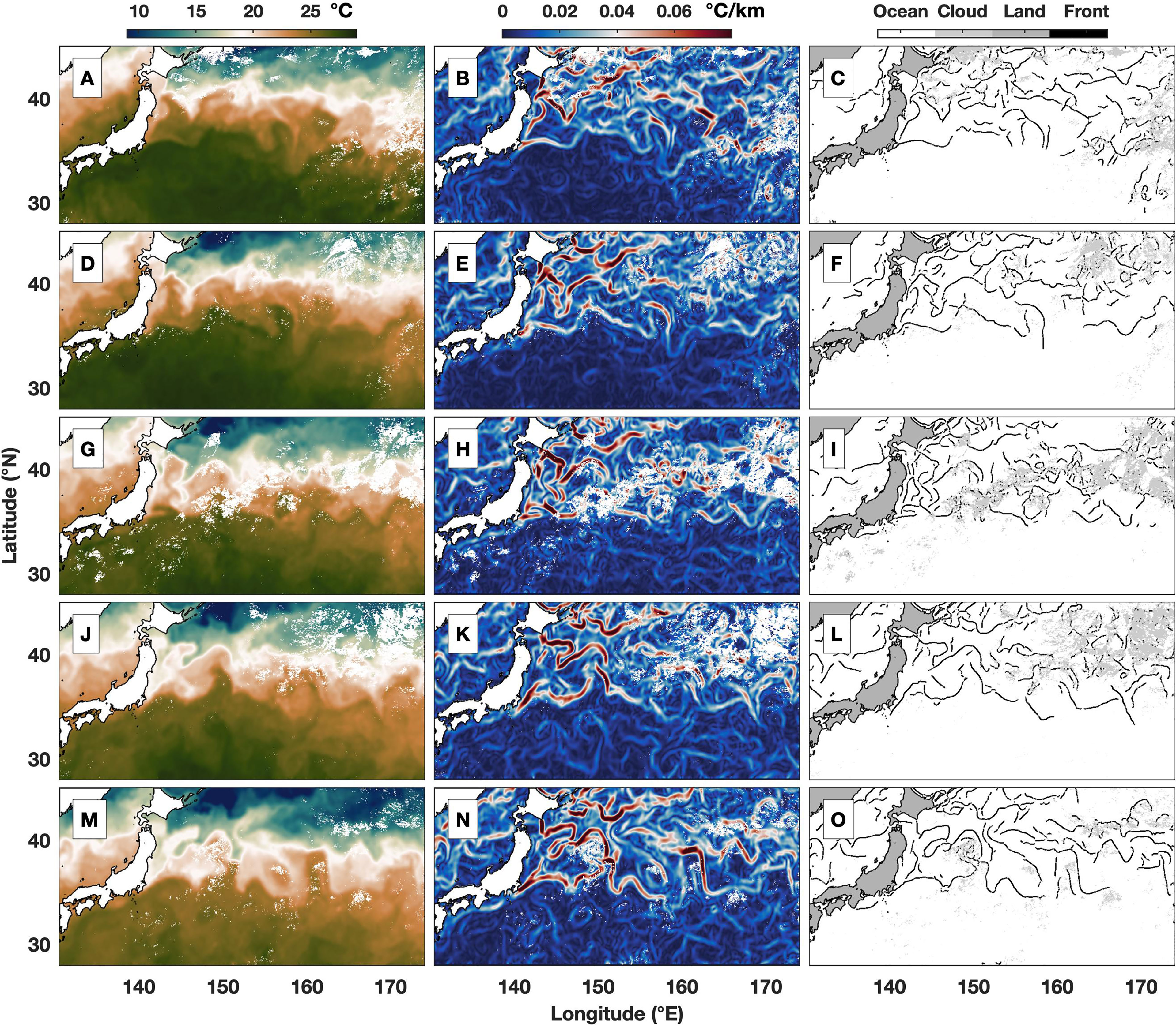
Figure 1 Example of sea surface temperature (SST) front detection using 11-day averaged (A, D, G, J, M) SST (°C), (B, E, H, K, N) SST gradient magnitude (°C/km), and (C, F, I, L, O) identified SST front. The middle time of average is (A–C) September 4, (D–F) September 15, (G–I) September 26, (J–L) October 7, and (M–O) October 18, 2002.

The monthly frontal features, including the averaged SST gradient magnitude (Figure 2A), frontal probability (Figure 2B) and frontal intensity (Figure 2C), in August 2008 are shown. The MFI shows high frontal intensity to the east of Japan in the zonal band at approximately 39°N (Figure 2C). The corresponding monthly frontal probability (Figure 2B) also shows high values in the same region. In comparison to a direct average of the gradient magnitude, the MFI is less noisy and is able to delineate high values in the SST gradient magnitude (Figure 2A). Because the frontal intensity is defined as zero if no fronts are identified during a certain month, the regions without fronts have a value close to zero (Figure 2C). In contrast, there is a persistent SST gradient value regardless of whether fronts are present (Figure 2A). Thus, the frontal intensity can effectively eliminate the influence of the background SST gradient by highlighting the front-associated features.

FIGURE 2

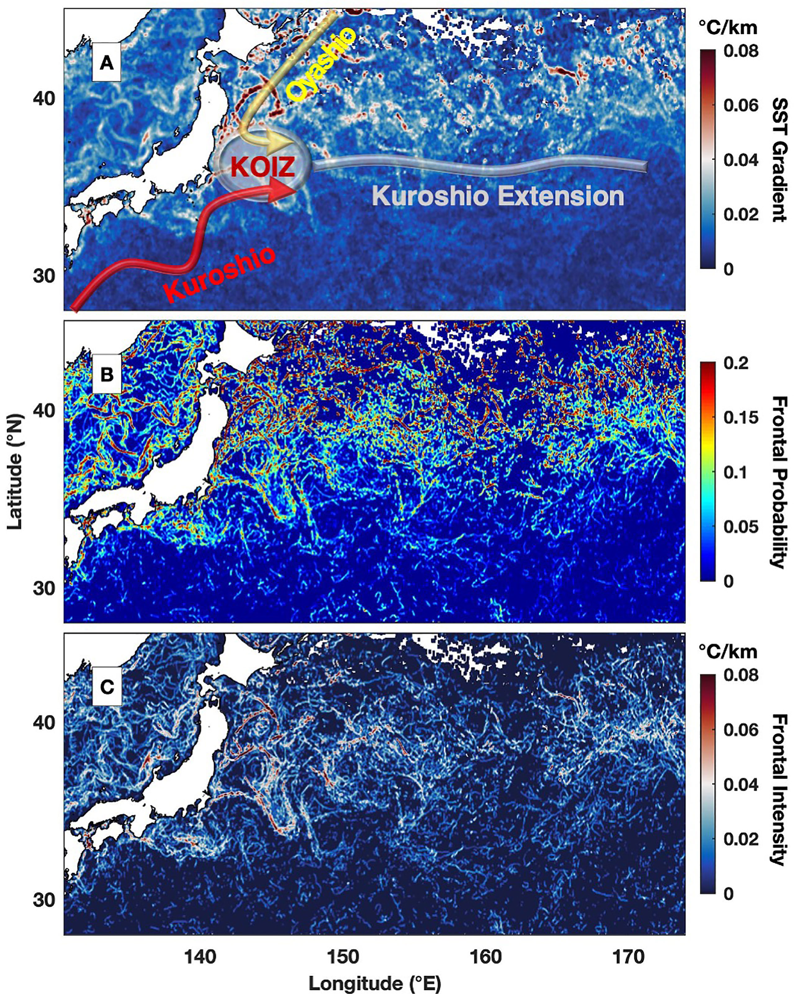
Figure 2 An example of monthly averaged (A) SST gradient (°C/km), (B) frontal probability and (C) frontal intensity (°C/km) in August 2008 for the Kuroshio Extension region. The blank area over the ocean indicates that the region is persistently obstructed by clouds during the month. The Kuroshio Current, Oyashio Current, Kuroshio-Oyashio Interfrontal Zone (KOIZ) and Kuroshio Extension are schematically shown in panel (A).

Average Frontal Features in the Kuroshio Extension

The frontal features in the Kuroshio Extension region are associated with prominent spatial and temporal variability. The spatial patterns of the overall SST gradient (Figure 3A), frontal probability (Figure 3B) and frontal intensity (Figure 3C) are highly similar. They are characterized by high values near the coast of Japan, particularly at approximately 40°N, and extend eastward, although the value generally decreases with offshore distance. As one of the strongest western boundary currents, the highest frontal probability and frontal intensity in the Kuroshio Extension are more than 9% and 0.03°C/km, respectively. These values are higher than those of eastern boundary currents (Wang et al., 2015) and some coastal upwelling regions (Wang et al., 2020), which are usually identified as the regions with prominent fronts (Belkin et al, 2009).

FIGURE 3

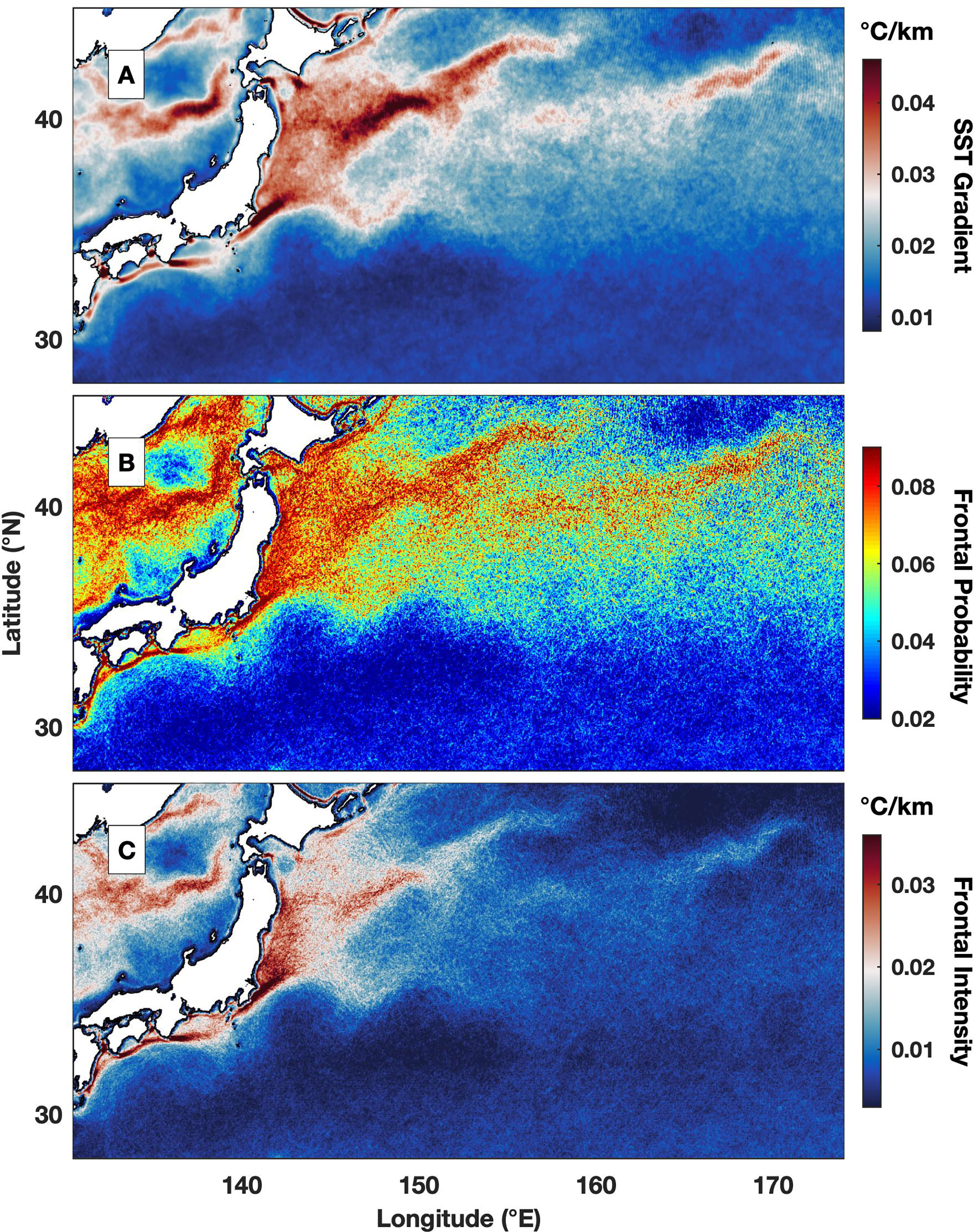
Figure 3 Seventeen-year averaged (A) SST gradient (°C/km), (B) frontal probability and (C) frontal intensity (°C/km) from September 2002 to August 2019.

There are also differences among the SST gradients, frontal probabilities and frontal intensities that were revealed in their overall distribution. For example, a large SST gradient, e.g., 0.04°C/km, exists in the entire Kuroshio Extension, while a high frontal probability, e.g., 8%, occupies an even larger area. In contrast, a high frontal intensity, e.g., 0.03°C/km, is concentrated in a small area characterized by a large SST gradient and high frontal probability. A large band of frontal intensity clearly delineates the KOIZ, where a high-value band can be found extending from the eastern coast of Japan, i.e., 35°N and 140°E, toward the northeast (Figure 3C). Thus, the frontal intensity can be used as a precise proxy that is little impacted by background SST gradients and fronts to describe frontal features and is further applied in the following analysis.

Seasonal Variability in Frontal Intensity

The seasonal averages of frontal intensity (where winter, spring, summer and fall are defined as December to February, March to May, June to August and September to November, respectively) show prominent differences (Figure 4). In winter, the region with a high frontal intensity is centralized in a small coastal area located directly to the east of Japan at approximately 35°N (Figure 4A). The corresponding value of frontal intensity is greater than 0.05°C/km, which is the highest of the year across the entire study region. In contrast, the fronts in the open ocean are much less pronounced, and the intensity values are generally close to zero. The frontal intensity in the Kuroshio Extension region is greatly enhanced in spring; in particular, frontal intensities greater than 0.03°C/km occupy the entire coastal area between 35°N and 41°N and extend approximately 400 km offshore (Figure 4B). The weakest frontal intensity occurs in summer, when the frontal intensity value is universally less than 0.02°C/km (Figure 4C), although weak fronts are distributed throughout the entire region. The frontal intensity greatly increases in the northern section, e.g., to the north of 35°N, during fall, and the corresponding value is approximately 0.03°C/km near the coastal region (Figure 4D). Simultaneously, the fronts are reduced in the southern region. There is also prominent seasonal variability in frontal intensity in the area to the west of Japan in the East Sea/Sea of Japan (Park et al., 2007); however, the underlying frontogenesis is related to eddies and the marginal sea circulation system, which is very different from the Kuroshio Extension, and the region is excluded from the current study.

FIGURE 4

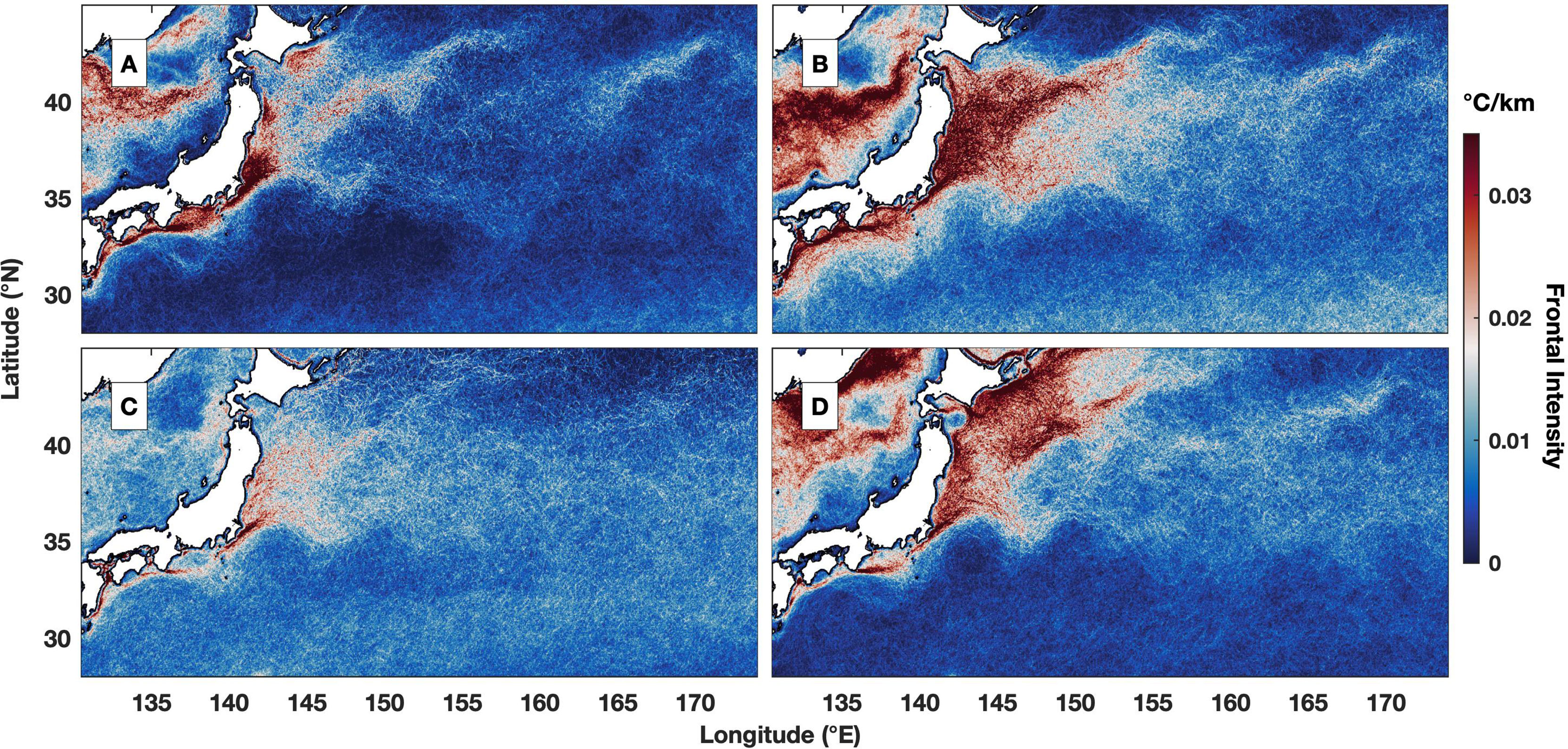
Figure 4 Seasonal averaged frontal intensity (°C/km) for (A) winter (December to February), (B) spring (March to May), (C) summer (June to August) and (D) fall (September to November).

The variability in MFI in the Kuroshio Extension is further investigated via EOFs. The first three modes explain approximately 15% of the total variance in the frontal intensity, e.g., 7.0%, 5.1% and 3.2% for EOF1, EOF2 and EOF3, respectively. The value is lower than many former studies that focused on frontal probability, where the first one or two modes usually explain 15% of the total variance (Wang et al., 2015). This finding is due to the complex dynamics in the Kuroshio Extension region, and the MFI has larger variation than frontal probability; thus, multiple modes are required to describe the variability in the MFI. The first EOF shows high intensity in the entire southern section of the study region, especially along the Kuroshio Current and Kuroshio Extension to the east of Japan (Figure 5A). The corresponding monthly average of the temporal EOF of MFI is dominated by a prominent seasonal variability, peaking in spring, e.g., March to May, and troughing in winter, e.g., December to February (Figure 5B). The enhancement in the MFI is highly consistent with the high seasonal average in spring (Figure 4B). The monthly average time series (Figures 5B, D, F) starts in December for easier comparison with Figure 4. Monthly average is near zero for the period from June to October, indicating the frontal intensity during this period is persistently close to the corresponding overall average. The second EOF mostly focuses on the northern section around the Oyashio Current (Figure 5C). The associated seasonal variability shows high frontal intensity in fall, e.g., September to November, and low intensity in summer, e.g., May to July (Figure 5D). The third mode of EOF delineates the frontal variability off the entire coast of Japan (Figure 5E). The corresponding time series shows elevated frontal intensity in winter and early spring, e.g., December to April, whereas depressed values occur in summer and early fall, e.g., June to October (Figure 5F). During winter, the temperature in the Kuroshio Current is much higher than that in the surroundings, thus generating stronger fronts (Seo et al., 2014). In contrast, almost the whole region features high temperatures during summer, and the horizontal gradient in SST is small, showing fewer fronts.

FIGURE 5

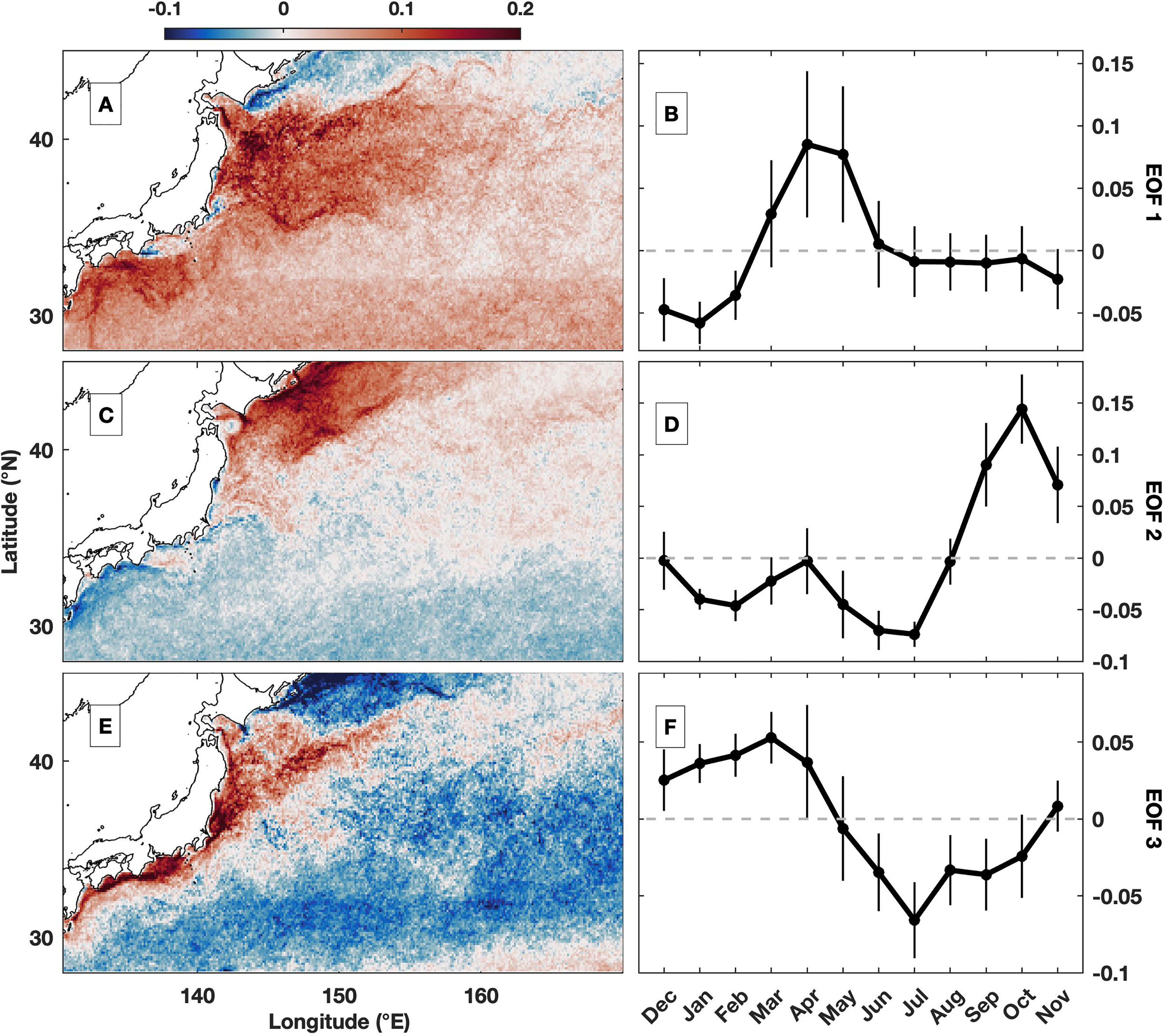
Figure 5 (A, C, E) Spatial magnitude and (B, D, F) temporal amplitude of monthly averaged frontal intensity (°C/km) using the empirical orthogonal function (EOF). The vertical bars in (B, D, F) indicate the standard deviation for corresponding months. The (A, B) first mode, (C, D) second mode and (E, F) third mode of EOFs. The monthly averaged time series in (B, D, F) is set to start in December for easier comparison with Figure 4.

The seasonality of frontal intensity varies among different regions, e.g., a fall peak in the northern section but a spring peak in the southern section (Figure 4), indicating that the underlying dynamics for frontogenesis are different or the seasonality varies. In Figure 6A, the regions with large variability in MFI, e.g., the coastal regions near Japan, Kuroshio Extension and branch of the Oyashio Current, are generally found in regions with high averages of frontal intensity (Figure 3C). A detailed comparison shows that there is actually large variability along the Kuroshio Current located south of Japan (31°N, 138°E). The area is highly consistent with the path of the Kuroshio Current (Qiu and Chen, 2010). The large variability indicates that multiple dynamics drive the variability in the front, which was formerly revealed by the EOFs in the Kuroshio Extension. However, the small amount of explained variance and large standard deviation in each month (Figures 5B, D, F) indicate that the temporal evolution also includes complex variability, such as noise in the MFI and interannual and intraseasonal variability. Thus, the MFI variance and the importance of the seasonal cycle at each location should be assessed first. The seasonal cycle is found to be important for the southern and northern regions, and their phases show maxima over the year in spring and fall, respectively, while the phase of annual maximum mainly occurs between May and July in the coastal region. Indeed, the identified seasonal cycles are consistent with the spatiotemporal features captured by EOFs (Figure 5). In comparison, the seasonal cycle in the majority of the region, especially around the Kuroshio Extension, e.g., between 32°N and 42°N, is not significant. This region is roughly the same region where a high magnitude of EOF1 was identified (Figure 5A), although the time series is mostly dominated by seasonal variation (Figure 5B). Thus, this finding can help to explain the low variance explained by the EOFs, as there are also signals characterized by other frequencies, e.g., interannual and intraseasonal variabilities.

FIGURE 6

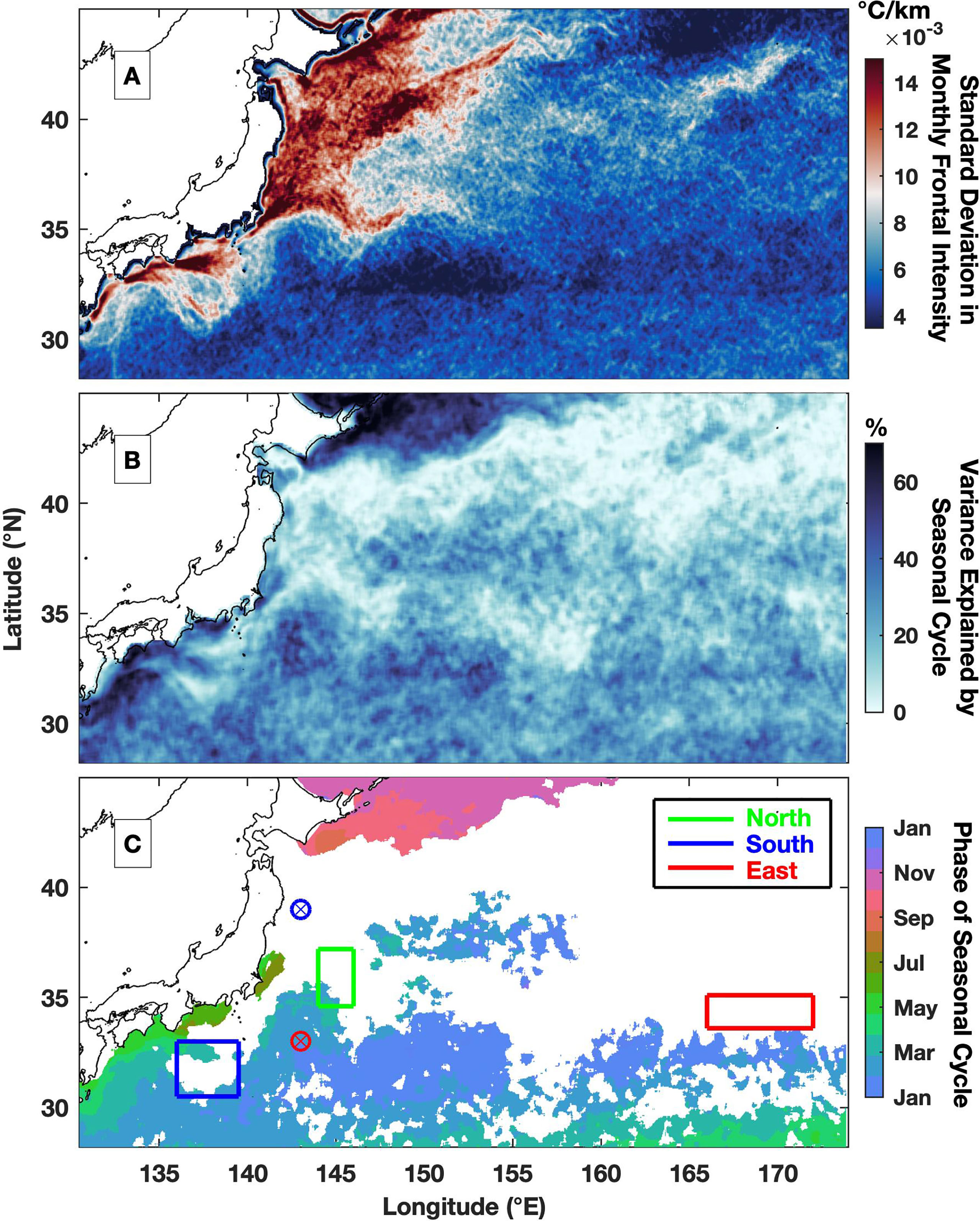
Figure 6 (A) Standard deviation of the monthly time series of MFI (°C/km). (B) Percentage of the variance explained by seasonal cycle. (C) Phase of the annual seasonal cycle of MFI; only the region with significant regression is shown. In panel (C), two locations denoted by blue and red circles are investigated in Figure 7, as the blue (red) location is dominated by a significant (nonsignificant) seasonal cycle. Three designated regions with nonsignificant seasonal cycles, i.e., north, south and east, are further applied to investigate interannual variability in Figure 9.

The percentage of variance explained by the seasonal cycle shows a significant dominance of the variability in MFI in the northern region (Figure 6B), and the corresponding phase of maximum in MFI happens in fall (Figure 6C). The southern region is also characterized by significant seasonal cycle, though the explained variance is only around 30%. The phase of maximum happens in winter in the eastern region and gradually change to later time of a year towards the west. Seasonal cycle contributes less than 20% of variance for majority of the Kuroshio Extension where the regression is not significant. Note the low value of explained seasonal cycle doesn’t imply the seasonal variability is not important, but the seasonal changes are not fitting well with the sinusoidal function. For example, the EOF1 captures the MFI is remaining a similar value around zeros for almost half year (Figure 5B), which cannot be reproduced with seasonal cycle. To further illustrate the significance of the seasonal cycle in MFI variation, two locations denoted in Figure 6C are selected as examples, and the corresponding seasonal cycles are obtained by fitting a sinusoidal function (Figure 7). In the northern region (denoted by the blue dot), the correlation between the seasonal cycle regression and the original time series is only 0.35 (Figure 7A), and the seasonal cycle is not significant at the 95% confidence level. The monthly average MFI actually captures two peaks, i.e., in April and October (Figure 7B). Simultaneously, there is large variance for each month, which is revealed by the high standard deviation. In comparison, the seasonal cycle is prominent in the southern region (denoted by the red dot), and its correlation with the original time series reaches 0.79 (Figure 7C), which is significant at the 95% confidence level. Additionally, the seasonal variability is clearly revealed by monthly averages, although the variation in each month is still high (Figure 7D) due to interannual variability; for example, lower magnitudes of the MFI are identified from 2010 to 2011, and higher magnitudes are identified in 2013 and from 2017 to 2019.

FIGURE 7

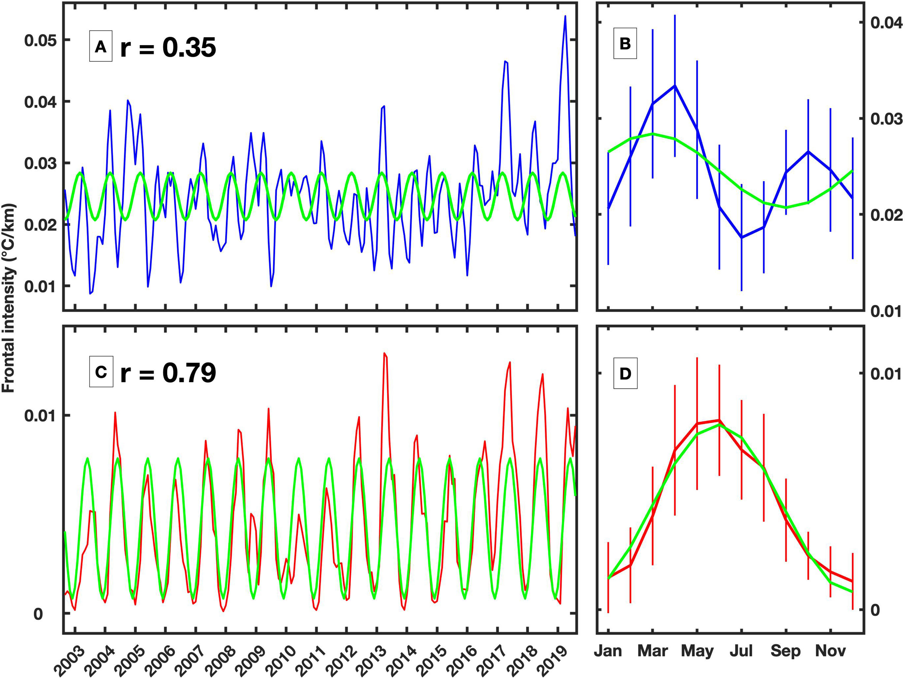
Figure 7 (A) Monthly time series of MFI in the blue region shown in Figure 6C. The green line shows the obtained seasonal cycle of the time series. The correlation coefficient between the monthly time series and seasonal cycles is shown in the figure. (B) Climatological monthly average and associated standard deviation. Panels (C, D) are similar to panels (A, B), respectively, but for the red region shown in Figure 6C.

Interannual Variability in Frontal Intensity

To investigate the migration and interannual variability in frontal intensity, the zonally averaged MFI is calculated between 166°E and 171°E (Figure 8A). The Hovmöller diagram shows that the fronts are first generated in the southern region and gradually develop in the northern region. This feature is better revealed in the field of monthly climatological averages (Figure 8B), in which fronts are generated in the southern region, e.g., 29°N, during spring and rapidly extend northward to 35°N until summer. The frontal intensity between 35°N and 41°N is simultaneously elevated in summer, while the frontal intensity in the northern section, e.g., at approximately 42°N, is generally high. The frontal intensity monotonically decreases from south, e.g., 0.015°C/km, to north, e.g., 0.008°C/km. Although the meridional migration of fronts is prominent, the value is much lower than that in coastal regions (Figure 3C). There is also clear interannual variability in the anomaly field, which is quantified by spatially averaging the MFI after removing the monthly climatological average (Figure 8C). The frontal intensity is low between mid-2006 and mid-2009 and between mid-2012 and 2015, while high values are found since. It is interesting to note that the negative anomalies are generally associated with the period when the Kuroshio Extension is characterized by an unstable mode (Qiu et al., 2014). This feature is quite different in the upstream of Kuroshio Extension where the variability in MFI is much larger during unstable mode (Figure 7C) associated with higher frontal probability (Wang et al., 2021b), but the underlying dynamic requires future investigation. The elevated frontal intensity after 2016 can be related to the occurrence of the Kuroshio Large Meander (Sugimoto et al., 2021), associated with the Kuroshio Extension switches to the unstable mode (Qiu et al., 2020), which introduces high instability (Nagano et al., 2019). Thus, fronts are characterized by complex dynamics, including seasonal and interannual variabilities. Similar enhancements in MFI after 2016 are also identified upstream of the Kuroshio Extension (Figure 7).

FIGURE 8

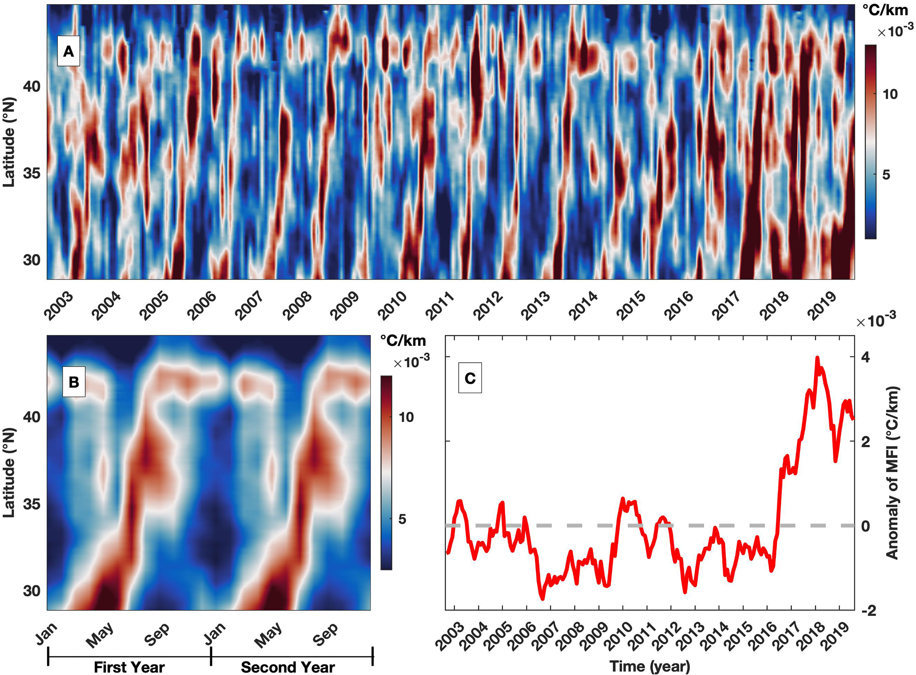
Figure 8 (A) Hovmöller diagram of MFI in the meridional direction for the region between 166°E and 171°E; (B) corresponding monthly climatology but repeated twice; (C) the time series of anomaly in MFI, which is obtained with the difference between the time series and corresponding climatology by averaging over the region.

The interannual variability in front is largely impacted by basin-scale signals, e.g., PDO and NPGO, especially in regions where the seasonal cycle is not significant (Figures 7A, B). Three regions with nonsignificant seasonal cycles are selected to investigate their interannual variability in frontal intensity (Figure 6C). The MFI in the northern region has a correlation of 0.59 with the NPGO, which leads the interannual variability in the MFI by 13 months. The positive phase of the NPGO enhances the frontal intensity along the Kuroshio Extension after roughly one year, and the negative NPGO depresses the frontal intensity (Figure 9A). The timing between the NPGO and MFI represents the time required for the signal to propagate from the eastern Pacific to the Kuroshio Extension (Lin et al., 2014). The MFIs in the southern and eastern regions are negatively correlated with the PDO, and the corresponding correlation coefficients are -0.55 (Figure 9B) and -0.65 (Figure 9C), respectively. All the acquired correlations are significant at the 95% confidence level. Notably, there is a difference in the time when the highest coefficients occur. The largest coefficient between frontal intensity and PDO occurs simultaneously in the south, but frontal intensity leads the PDO by 6 months in the east. The timing indicates a westward propagation of frontal intensities that initiates in the east around the Kuroshio Extension and propagates west toward the Kuroshio Current. A similar westward propagation signal was identified in previous studies that found that the interannual variability in the SST gradient is modulated by the PDO signal, and its different phases induce changes in the stability of the Kuroshio Extension (Wang et al., 2021b). Other interannual signals are also investigated, such as ENSO and AMO, but no significant dependence is found between these signals and the frontal intensity.

FIGURE 9

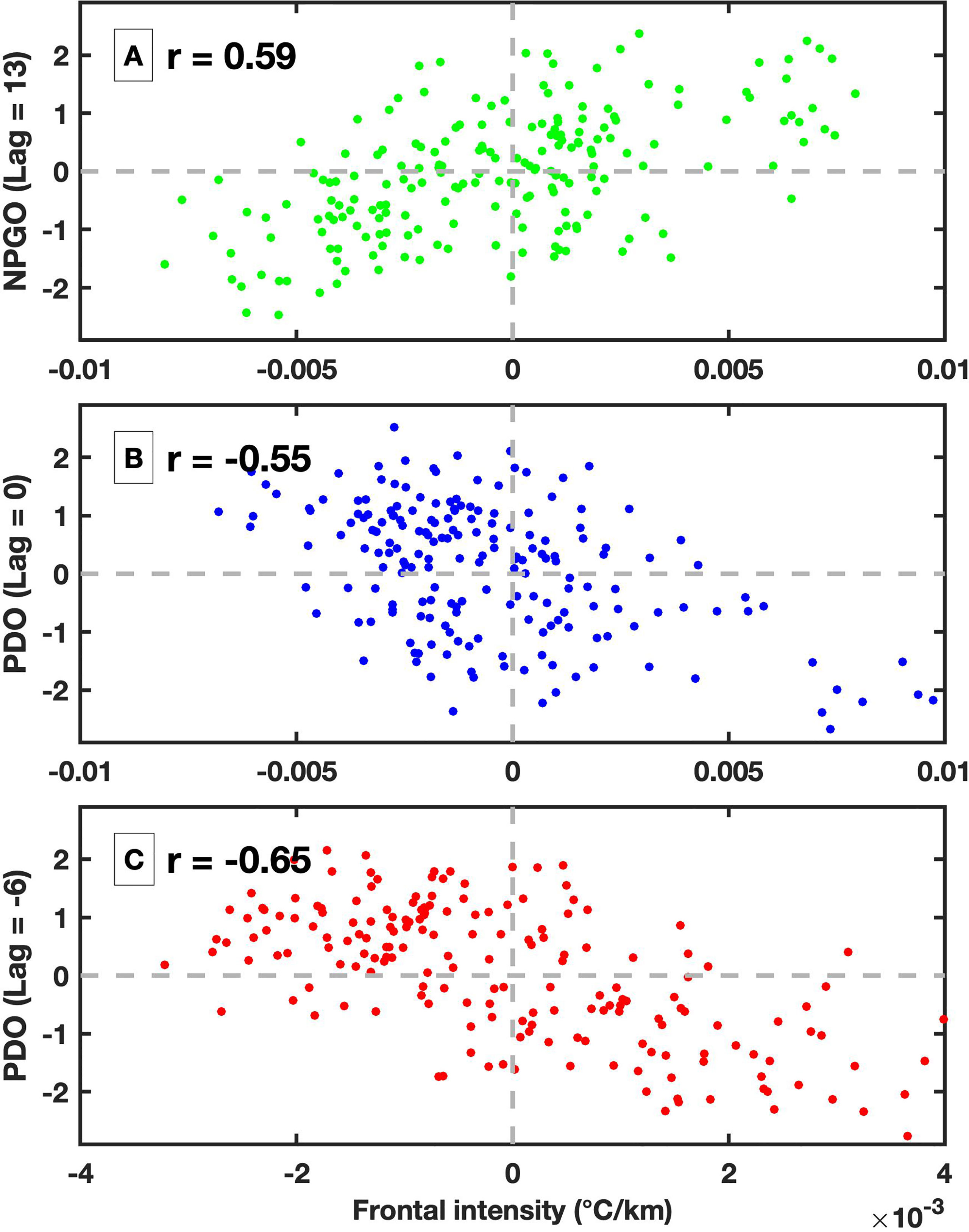
Figure 9 Scatterplot between (A) MFI in the northern region and NPGO index where the NPGO is leading by 13 months; (B) MFI in the southern region and PDO index without lagging; (C) MFI in the eastern region and PDO index where the MFI is leading by 6 months. The applied lag is selected to obtain the largest correlation between two time series. All the correlations are significant at the 95% confidence level. The regions are denoted in Figure 6C.

Discussion

Seventeen years of satellite observations of SST are applied to detect oceanic fronts and the associated features, i.e., frontal intensity, in the region of the Kuroshio Extension. During the front detection procedure, the SST gradient is first calculated, and the front is identified based on the direction and value of the SST gradient (Wang et al., 2020). The applied method can successfully capture the location of fronts (Figure 1), which are mainly distributed along the Kuroshio Extension and the region to the north. Due to the contrasting features of the Kuroshio Current and Oyashio Current, their confluence is characterized by strong dynamics (Miyazawa et al., 2009). Indeed, prominent frontal intensities are identified in the region of the KOIZ (Vivier et al., 2020). The large frontal intensities in the northern region (Figure 3) are related to the strong mesoscale eddies (Ji et al., 2018) and oscillation in the path of the Oyashio Current (Wu et al., 2019). In particular, the two identified bands, e.g., 40°N, 150°E and 40°N, 168°E, distributed toward the northeast are in good agreement with the persistent anticyclonic eddy and the flow of the subarctic current, which flows toward the northeast between 40°N and 43°N (Ohshima et al., 2005).

In comparison, frontal intensities are much less prominent in the southern section, with sparse and weaker fronts occurring during spring and summer (Figure 4). The region is a part of the North Pacific subtropical gyre (McClain et al., 2004), where the surface water is uniformly high in temperature (Kobashi and Kubokawa, 2012). Frontal intensities are elevated in the region located further south at the subtropical front between 20°N and 25°N (Yuan and Talley, 1996), but this feature is not included in the current study. During spring and summer, the North Pacific subtropical gyre shifts northward in association with the presence of fronts in the southern section of the study region. The meridional migration of fronts is also observed in Figures 8A, B, spanning from spring to summer.

Previous studies have focused on frontal distribution and probability (Yuan and Talley, 1996); however, some fronts are distributed persistently at certain positions, and the location provides limited information for describing the frontal features (Freeman et al., 2016). A similar phenomenon is identified when the confluence of the Kuroshio Current and Oyashio Current introduces a persistent front in the Kuroshio Extension region. Thus, frontal intensity offers new insight for understanding frontal features and for investigating underlying frontogenesis. For example, the background SST gradient exists universally in the ocean and can be interpreted as many weak fronts (Figure 2A). In comparison, the frontal intensity is defined only when the location is identified as a front; thus, the background SST gradient is greatly reduced, and the frontal features are more prominent (Figure 2C).

The first three EOF modes all reveal prominent seasonal variability in the MFI (Figure 5). The region with the highest frontal intensity shifts meridionally during different seasons (Figure 4) due to the trade wind’s expansion and migration of the confluence zone (Wu et al., 2020). Although most former studies describe frontal variability using seasonal cycles (Chen et al., 2019), the current study shows that there are also other forms of variance, such as intraseasonal (Figure 7) and interannual variabilities (Figure 8). The seasonal cycle is not a significant pattern for the MFI in the Kuroshio Extension (Figure 6C). A detailed investigation found that the variability is much more complex and that the seasonal cycle does not explain the total variability. Because of the influence of interannual signals on modulating frontal variability (Wang et al., 2020), the MFI in the region with a nonsignificant seasonal cycle (Figure 6C) is characterized by complex variability (Figure 7A).

Due to the complex dynamics in the Kuroshio Extension region, it is difficult to delineate the frontal intensity with simplified signals. Moreover, fronts are actually three-dimensional features (Wu et al., 2019), and the subsurface information is also important to describe the comprehensive features of fronts. With the development of automatic oceanic observation platforms, e.g., unmanned surface vehicles, Argo floats, and gliders (Chai et al., 2020), the vertical section on both sides of the front can be measured to better describe the differences in oceanic features across the front and associated dynamics (Shao et al., 2019).

The convergence associated with fronts aggregates and elevates nutrient levels, which can subsequently induce ecosystem responses (Woodson and Litvin, 2015). Clear dependence was previously identified between fronts and marine phytoplankton in response to both seasonal and interannual variabilities (Kouketsu et al., 2016). The Kuroshio Extension has been an important fishing ground due to its high productivity (Watanabe, 2009). Thus, an improved knowledge of oceanic fronts is helpful to understand the variability in marine primary production and the carbon cycle.

Conclusion

Satellite-derived frontal features are investigated in the Kuroshio Extension region. Seasonal cycles are generally a critical component for all geophysical features, i.e., SST, SST gradients and fronts; thus, they are widely applied to describe signals. However, our study indicates that it is important to evaluate whether the seasonal cycle is significant beforehand (Figure 6), as the variability in signals can be much more complex (Figure 7). A simplified seasonal cycle can be misleading when the signal is influenced at different scales, i.e., intraseasonal and interannual variability. The MFI is a good parameter to delineate the spatial and temporal variability in fronts that can reduce the background noise in the SST gradient field.

A major focus is to describe the seasonal and interannual variability in frontal intensity in the Kuroshio Extension and investigate the underlying dynamics that drive the corresponding variability. The seasonal variability in the MFI is mostly impacted by the confluence of the Kuroshio and Oyashio currents (Kida et al., 2015) and associated mesoscale dynamics, such as eddies (Itoh and Yasuda, 2010; Chelton et al., 2011). The interannual variability is impacted by basin-scale signals, such as the PDO and NPGO (Wang et al., 2021b). Due to the importance of the Kuroshio Extension in driving the carbon cycle and fisheries (Kitagawa et al., 2004; Yatsu et al., 2013; Sutton et al., 2017), an improved understanding of frontal intensity is crucial for predicting the changes in ocean dynamics and ecosystems under the scenario of future climate change.

Data Availability Statement

The original contributions presented in the study are included in the article. Further inquiries can be directed to the corresponding author.

Author Contributions

Data curation, JX. Writing, YW and JX. Review of the manuscript, ZF, YL, and XG. Visualization, YL. Funding, YW. All authors have read and agreed to the published version of the manuscript.

Funding

The study is funded by the National Natural Science Foundation of China (42176013, 41730536 and 41890805).

Conflict of Interest

The authors declare that the research was conducted in the absence of any commercial or financial relationships that could be construed as a potential conflict of interest.

Publisher’s Note

All claims expressed in this article are solely those of the authors and do not necessarily represent those of their affiliated organizations, or those of the publisher, the editors and the reviewers. Any product that may be evaluated in this article, or claim that may be made by its manufacturer, is not guaranteed or endorsed by the publisher.

Acknowledgments

We are very thankful to the National Aeronautics and Space Administration (NASA) for producing and distributing the sea surface temperature dataset (NASA, 2014).

References

Belkin I. M. (2021). Remote Sensing of Ocean Fronts in Marine Ecology and Fisheries. Remote Sens. 13, 883. doi: 10.3390/rs13050883

CrossRef Full Text | Google Scholar

Belkin I. M., Cornillon P. C., Sherman K. (2009). Fronts in Large Marine Ecosystems. Prog. Oceanogr. 81, 223–236. doi: 10.1016/j.pocean.2009.04.015

CrossRef Full Text | Google Scholar

Canny J. A. (1986). Computational Approach to Edge Detection. IEEE Trans. Pattern Anal. Mach. Intell. 8, 679–698. doi: 10.1109/TPAMI.1986.4767851

PubMed Abstract | CrossRef Full Text | Google Scholar

Castelao R. M., Wang Y. (2014). Wind-Driven Variability in Sea Surface Temperature Front Distribution in the California Current System. J. Geophys. Res. Oceans 119, 1861–1875. doi: 10.1002/2013JC009531

CrossRef Full Text | Google Scholar

Cayula J., Cornillon P. (1996). Cloud Detection From a Sequence of SST Images. Remote Sens. Environ. 55, 80–88. doi: 10.1016/0034-4257(95)00199-9

CrossRef Full Text | Google Scholar

Chai F., Kenneth J., Claustre H., Xing X., Wang Y., Boss E., et al. (2020). Monitoring Ocean Biogeochemistry With Autonomous Platforms. Nat. Rev. Earth Environ. 1 (6), 315–326. doi: 10.1038/s43017-020-0053-y

CrossRef Full Text | Google Scholar

Chelton D. B., Gaube P., Schlax M. G., Early J. J., Samelson R. M. (2011). The Influence of Nonlinear Mesoscale Eddies on Near-Surface Oceanic Chlorophyll. Science 334 (6054), 328–332. doi: 10.1126/science.1208897

PubMed Abstract | CrossRef Full Text | Google Scholar

Chen H. H., Qi Y., Wang Y., Chai F. (2019). Seasonal Variability of SST Fronts and Winds on the Southeastern Continental Shelf of Brazil. Ocean Dyn. 69 (11), 1387–1399. doi: 10.1007/s10236-019-01310-1

CrossRef Full Text | Google Scholar

Clayton S., Nagai T., Follows M. J. (2014). Fine Scale Phytoplankton Community Structure Across the Kuroshio Front. J. Plankton Res. 36 (4), 1017–1030. doi: 10.1093/plankt/fbu020

CrossRef Full Text | Google Scholar

Clayton S., Palevsky H. I., Thompson L., Quay P. D. (2021). Synoptic Mesoscale to Basin Scale Variability in Biological Productivity and Chlorophyll in the Kuroshio Extension Region. J. Geophys. Res. Oceans 126, e2021JC017782. doi: 10.1029/2021JC017782

CrossRef Full Text | Google Scholar

Freeman N. M., Lovenduski N. S., Gent P. R. (2016). Temporal Variability in the Antarctic Polar Front, (2002–2014). J. Geophys. Res. Oceans 121, 7263–7276. doi: 10.1002/2016JC012145

CrossRef Full Text | Google Scholar

Gan J., Allen J. S. (2002). A Modeling Study of Shelf Circulation Off Northern California in the Region of the Coastal Ocean Dynamics Experiment: Response to Relaxation of Upwelling Winds. J. Geophys. Res. Oceans 107, 3123. doi: 10.1029/2000JC000768

CrossRef Full Text | Google Scholar

Graham R. M., De Boer A. M. (2013). The Dynamical Subtropical Front. J. Geophys. Res. Oceans 118, 5676– 5685. doi: 10.1002/jgrc.20408

CrossRef Full Text | Google Scholar

Guo X., Zhu X.-H., Wu Q.-S., Huang D. (2012). The Kuroshio Nutrient Stream and its Temporal Variation in the East China Sea. J. Geophys. Res. 117, C01026. doi: 10.1029/2011JC007292

CrossRef Full Text | Google Scholar

Hashioka T., Yamanaka Y. (2007). Seasonal and Regional Variations of Phytoplankton Groups by Top-Down and Bottom-Up Controls Obtained by a 3D Ecosystem Model. Ecol. Modell. 202 (1–2), 68–80. doi: 10.1016/j.ecolmodel.2006.05.038

CrossRef Full Text | Google Scholar

Itoh S., Yasuda I. (2010). Characteristics of Mesoscale Eddies in the Kuroshio-Oyashio Extension Region Detected From the Distribution of the Sea Surface Height Anomaly. J. Phys. Oceanogr. 40 (5), 1018–1034. doi: 10.1175/2009JPO4265.1

CrossRef Full Text | Google Scholar

Ji J., Dong C., Zhang B., Liu Y., Zou B., King G. P., et al. (2018). Oceanic Eddy Characteristics and Generation Mechanisms in the Kuroshio Extension Region. J. Geophys. Res. Oceans 123, 8548–8567. doi: 10.1029/2018JC014196

CrossRef Full Text | Google Scholar

Kartushinsky A. V., Sidorenko A. Y. (2013). Analysis of the Variability of Temperature Gradient in the Ocean Frontal Zones Based on Satellite Data. Adv. Space Res. 52 (8), 1467–1475. doi: 10.1016/j.asr.2013.07.023

CrossRef Full Text | Google Scholar

Kida S., Mitsudera H., Aoki S., Guo X., Ito S. I., Kobashi F., et al. (2015). Oceanic Fronts and Jets Around Japan: A Review. J. Oceanogr. 71, 469–497. doi: 10.1007/978-4-431-56053-1_1

CrossRef Full Text | Google Scholar

Kitagawa T., Kimura S., Nakata H., Yamada H. (2004). Diving Behavior of Immature, Feeding Pacific Bluefin Tuna (Thunnus Thynnus Orientalis) in Relation to Season and Area: The East China Sea and the Kuroshio-Oyashio Transition Region. Fish. Oceanogr. 13 (3), 161–180. doi: 10.1111/j.1365-2419.2004.00282.x

CrossRef Full Text | Google Scholar

Kobashi F., Kubokawa A. (2012). Review on North Pacific Subtropical Countercurrents and Subtropical Fronts: Role of Mode Waters in Ocean Circulation and Climate. J. Oceanogr. 68 (1), 21–43. doi: 10.1007/s10872-011-0083-7

CrossRef Full Text | Google Scholar

Kostianoy A. G., Ginzburg A. I., Frankignoulle M., Delille B. (2004). Fronts in the Southern Indian Ocean as Inferred From Satellite Sea Surface Temperature Data. J. Mar. Syst. 45 (1–2), 55–73. doi: 10.1016/j.jmarsys.2003.09.004

CrossRef Full Text | Google Scholar

Kouketsu S., Kaneko H., Okunishi T., Sasaoka K., Itoh S., Inoue R., et al. (2016). Mesoscale Eddy Effects on Temporal Variability of Surface Chlorophyll a in the Kuroshio Extension. J. Oceanogr. 72 (3), 439–451. doi: 10.1007/s10872-015-0286-4

CrossRef Full Text | Google Scholar

Legeckis R. (1978). A Survey of Worldwide Sea Surface Temperature Fronts Detected by Environmental Satellites. J. Geophys. Res. Oceans 83 (C9), 4501–4522. doi: 10.1029/JC083iC09p04501

CrossRef Full Text | Google Scholar

Lin P., Chai F., Xue H., Xiu P. (2014). Modulation of Decadal Oscillation on Surface Chlorophyll in the Kuroshio Extension. J. Geophys. Res. Oceans 119, 187–199. doi: 10.1002/2013JC009359

CrossRef Full Text | Google Scholar

Long Y., Zhu X.-H., Guo X. (2019). The Oyashio Nutrient Stream and its Nutrient Transport to the Mixed Water Region. Geophys. Res. Lett. 46, 1513–1520. doi: 10.1029/2018GL081497

CrossRef Full Text | Google Scholar

Lorenzzetti J. A., Stech J. L., Mello Filho W. L., Assireu A. T. (2009). Satellite Observation of Brazil Current Inshore Thermal Front in the SW South Atlantic: Space/time Variability and Sea Surface Temperatures. Conti. Shelf Res. 29 (17), 2061–2068. doi: 10.1016/j.csr.2009.07.011

CrossRef Full Text | Google Scholar

McClain C. R., Signorini S. R., Christian J. R. (2004). Subtropical Gyre Variability Observed by Ocean-Color Satellites. Deep Sea Res. Part II Top. Stud. Oceanogr. 51 (1–3), 281–301. doi: 10.1016/j.dsr2.2003.08.002

CrossRef Full Text | Google Scholar

Miller P. I. (2009). Composite Front Maps for Improved Visibility of Dynamic Sea-Surface Features on Cloudy SeaWiFS and AVHRR Data. J. Mar. Syst. 78, 327–336. doi: 10.1016/j.jmarsys.2008.11.019

CrossRef Full Text | Google Scholar

Miyazawa Y., Zhang R., Guo X., Tamura H., Ambe D., Lee J. S., et al. (2009). Water Mass Variability in the Western North Pacific Detected in a 15-Year Eddy Resolving Ocean Reanalysis. J. Oceanogr. 65 (6), 737–756. doi: 10.1007/s10872-009-0063-3

CrossRef Full Text | Google Scholar

Nagai T., Clayton S. (2017). Nutrient Interleaving Below the Mixed Layer of the Kuroshio Extension Front. Ocean Dyn. 67 (8), 1027–1046. doi: 10.1007/s10236-017-1070-3

CrossRef Full Text | Google Scholar

Nagano A., Yamashita Y., Hasegawa T., Ariyoshi K., Matsumoto H., Shinohara M. (2019). Characteristics of an Atypical Large−Meander Path of the Kuroshio Current South of Japan Formed in September 2017. Mar. Geophys. Res. 40, 525–539. doi: 10.1007/s11001-018-9372-5

CrossRef Full Text | Google Scholar

NASA (2014). Goddard Space Flight Center, Ocean Ecology Laboratory, Ocean Biology Processing Group. Moderate-Resolution Imaging Spectroradiometer (MODIS) Aqua 11µm Day/Night Sea Surface Temperature Data (Greenbelt, MD, USA: NASA OB.DAAC).

Google Scholar

Ohshima K. I., Wakatsuchi M., Saitoh S. I. (2005). Velocity Field of the Oyashio Region Observed With Satellite-Tracked Surface Drifters During 1999–2000. J. Oceanogr. 61 (5), 845–855. doi: 10.1007/s10872-006-0004-3

CrossRef Full Text | Google Scholar

Parfitt R., Czaja A., Minobe S., Kuwano-Yoshida A. (2016). The Atmospheric Frontal Response to SST Perturbations in the Gulf Stream Region. Geophys. Res. Lett. 43, 2299–2306. doi: 10.1002/2016GL067723

CrossRef Full Text | Google Scholar

Park K. A., Ullman D. S., Kim K., Chung J. Y., Kim K. R. (2007). Spatial and Temporal Variability of Satellite-Observed Subpolar Front in the East/Japan Sea. Deep Sea Res. Part I: Oceanogr. Res. Pap. 54 (4), 453–470. doi: 10.1016/j.dsr.2006.12.010

CrossRef Full Text | Google Scholar

Qiu B., Chen S. (2010). Eddy-Mean Flow Interaction in the Decadally Modulating Kuroshio Extension System. Deep Sea Res. Part II Top. Stud. Oceanogr. 57 (13–14), 1098–1110. doi: 10.1016/j.dsr2.2008.11.036

CrossRef Full Text | Google Scholar

Qiu B., Chen S., Schneider N., Oka E., Sugimoto S. (2020). On the Reset of the Wind-Forced Decadal Kuroshio Extension Variability in Late 2017. J. Clim. 33, 10813–10828. doi: 10.1175/JCLI-D-20-0237.1

CrossRef Full Text | Google Scholar

Qiu B., Chen S., Schneider N., Taguchi B. (2014). A Coupled Decadal Prediction of the Dynamic State of the Kuroshio Extension System. J. Clim. 27 (4), 1751–1764. doi: 10.1175/JCLI-D-13-00318.1

CrossRef Full Text | Google Scholar

Qu T., Mitsudera H., Qiu B. (2001). A Climatological View of the Kuroshio/Oyashio System East of Japan. J. Phys. Oceanogr. 31, 2575–2589. doi: 10.1175/1520-0485(2001)031<2575:ACVOTK>2.0.CO;2

CrossRef Full Text | Google Scholar

Ribalet F., Marchetti A., Hubbard K., Brown K., Durkin C., Morales R., et al. (2010). Unveiling a Phytoplankton Hotspot at a Narrow Boundary Between Coastal and Offshore Waters. Proc. Natl. Acad. Sci. U.S.A. 107, 16571–16576. doi: 10.1073/pnas.1005638107

PubMed Abstract | CrossRef Full Text | Google Scholar

Seo Y., Sugimoto S., Hanawa K. (2014). Long-Term Variations of the Kuroshio Extension Path in Winter: Meridional Movement and Path State Change. J. Clim. 27, 5929–5940. doi: 10.1175/JCLI-D-13-00641.1

CrossRef Full Text | Google Scholar

Shan X., Jing Z., Gan B., Wu L., Chang P., Ma X., et al. (2020). Surface Heat Flux Induced by Mesoscale Eddies Cools the Kuroshio-Oyashio Extension Region. Geophys. Res. Lett. 47 (1), e2019GL086050. doi: 10.1029/2019GL086050

CrossRef Full Text | Google Scholar

Shao M., Ortiz-Suslow D. G., Haus B. K., Lund B., Williams N. J., Özgökmen T. M., et al. (2019). The Variability of Winds and Fluxes Observed Near Submesoscale Fronts. J. Geophys. Res. Oceans 124 (11), 7756–7780. doi: 10.1029/2019JC015236

CrossRef Full Text | Google Scholar

Simpson J. J. (1990). On the Accurate Detection and Enhancement of Oceanic Features Observed in Satellite Data. Remote Sens. Environ. 33 (1), 17–33. doi: 10.1016/0034-4257(90)90052-N

CrossRef Full Text | Google Scholar

Sugimoto S., Kobayashi N., Hanawa K. (2014). Quasi-Decadal Variation in Intensity of the Western Part of the Winter Subarctic SST Front in the Western North Pacific: The Influence of Kuroshio Extension Path State. J. Phys. Oceanogr. 44, 2753–2762. doi: 10.1175/JPO-D-13-0265.1

CrossRef Full Text | Google Scholar

Sugimoto S., Qiu B., Schneider N. (2021). Local Atmospheric Response to the Kuroshio Large Meander Path in Summer and Its Remote Influence on the Climate of Japan. J. Clim. 34 (9), 3571–3589. doi: 10.1175/JCLI-D-20-0387.1

CrossRef Full Text | Google Scholar

Sutton A. J., Wanninkhof R., Sabine C. L., Feely R. A., Cronin M. F., Weller R. A. (2017). Variability and Trends in Surface Seawater Pco2 and CO2 Flux in the Pacific Ocean. Geophys. Res. Lett. 44 (11), 5627–5636. doi: 10.1002/2017GL073814

CrossRef Full Text | Google Scholar

Ullman D. S., Cornillon P. C. (2000). Evaluation of Front Detection Methods for Satellite-Derived SST Data Using in Situ Observations. J. Atmos. Ocean. Technol. 17 (12), 1667–1675. doi: 10.1175/1520-0426(2000)017<1667:EOFDMF>2.0.CO;2

CrossRef Full Text | Google Scholar

Vivier F., Kelly K., Thompson L. (2020). Heat Budget in the Kuroshio Extension Region: 1993–99. J. Phys. Oceanogr. 32, 3436–3454. doi: 10.1175/1520-0485(2002)032<3436:HBITKE>2.0.CO;2

CrossRef Full Text | Google Scholar

Wang Y., Castelao R. M., Yuan Y. (2015). Seasonal Variability of Alongshore Winds and Sea Surface Temperature Fronts in Eastern Boundary Current Systems. J. Geophys. Res. Oceans 120, 2385–2400. doi: 10.1002/2014JC010379

CrossRef Full Text | Google Scholar

Wang Y., Liu J., Liu H., Lin P., Yuan Y., Chai F. (2021a). Seasonal and Interannual Variability in the Sea Surface Temperature Front in the Eastern Pacific Ocean. J. Geophys. Res. Oceans 126, e2020JC016356. doi: 10.1029/2020JC016356

CrossRef Full Text | Google Scholar

Wang Y., Tang R., Yu Y., Ji F. (2021b). Variability in the Sea Surface Temperature Gradient and Its Impacts on Chlorophyll-A Concentration in the Kuroshio Extension. Remote Sens. 13 (5), 888. doi: 10.3390/rs13050888

CrossRef Full Text | Google Scholar

Wang Y., Yu Y., Zhang Y., Chai F. (2020). Distribution and Variability of Sea Surface Temperature Fronts in the South China Sea. Estuar. Coast. Shelf Sci. 240, 106793. doi: 10.1016/j.ecss.2020.106793

CrossRef Full Text | Google Scholar

Watanabe Y. (2009). Recruitment Variability of Small Pelagic Fish Populations in the Kuroshio-Oyashio Transition Region of the Western North Pacific. J. North Atl. Fish. Sci. 41, 197–204. doi: 10.2960/J.v41.m635

CrossRef Full Text | Google Scholar

Woodson C., Litvin S. (2015). Ocean Fronts Drive Marine Fishery Production and Biogeochemical Cycling. Proc. Natl. Acad. Sci. U.S.A. 112 (6), 1710–1715. doi: 10.1073/pnas.1417143112

PubMed Abstract | CrossRef Full Text | Google Scholar

Wu B., Lin X., Qiu B. (2019). On the Seasonal Variability of the Oyashio Extension Fronts. Clim. Dyn. 53 (11), 7011–7025. doi: 10.1007/s00382-019-04972-1

CrossRef Full Text | Google Scholar

Wu B., Lin X., Yu L. (2020). North Pacific Subtropical Mode Water is Controlled by the Atlantic Multidecadal Variability. Nat. Clim. Change 10 (3), 238–243. doi: 10.1038/s41558-020-0692-5

CrossRef Full Text | Google Scholar

Yasuda I. (2003). Hydrographic Structure and Variability in the Kuroshio-Oyashio Transition Area. J. Oceanogr. 59 (4), 389–402. doi: 10.1023/A:1025580313836

CrossRef Full Text | Google Scholar

Yatsu A., Chiba S., Yamanaka Y., Ito S., Shimizu Y., Kaeriyama M., et al. (2013). Climate Forcing and the Kuroshio/Oyashio Ecosystem. ICES. J. Mar. Sci. 70, 922–933. doi: 10.1093/icesjms/fst084

CrossRef Full Text | Google Scholar

Yoder J. A., Ackleson S. G., Barber R. T., Flament P., Balch W. M. (1994). A Line in the Sea. Nature 371, 689–692. doi: 10.1038/371689a0

CrossRef Full Text | Google Scholar

Yuan Y., Castelao R. M. (2017). Eddy-Induced Sea Surface Temperature Gradients in Eastern Boundary Current Systems. J. Geophys. Res. Oceans 122 (6), 4791–4801. doi: 10.1002/2017jc012735

CrossRef Full Text | Google Scholar

Yuan X., Talley L. D. (1996). The Subarctic Frontal Zone in the North Pacific: Characteristics of Frontal Structure From Climatological Data and Synoptic Surveys. J. Geophys. Res. Oceans 101 (C7), 16491–16508. doi: 10.1029/96JC01249

CrossRef Full Text | Google Scholar

Yu Y., Wang Y., Cao L., Chai F. (2020). The Ocean-Atmosphere Interaction Over a Summer Upwelling System in the South China Sea. J. Mar. Syst. 208, 103360. doi: 10.1016/j.jmarsys.2020.103360

CrossRef Full Text | Google Scholar

Yu Y., Xing X., Liu H., Yuan Y., Wang Y., Chai F. (2019). The Variability of Chlorophyll-a and its Relationship With Dynamic Factors in the Basin of the South China Sea. J. Mar. Syst. 200, 103230. doi: 10.1016/j.jmarsys.2019.103230

CrossRef Full Text | Google Scholar