CGAN Based Improved ASI Retrieval Algorithm for Antarctic Sea Ice Concentration

1 Introduction

The polar region is an important indicator of global climate. With the increasing severity of global warming, sea ice is an important climate factor in the polar region, and the monitoring and the studies of sea ice have attracted more and more attention. Sea ice concentration is the most intuitive parameter to study the sea ice change. Sea ice concentration plays an important role in the monitoring and prediction of sea ice change, and it is of great significance to study global climate change. Passive microwave data is not limited by day and night, which is less affected by clouds and fog, and it has good temporal and spatial continuity. Passive microwave data have been used extensively for polar sea ice monitoring. Sea ice concentration can provide reliable basic data and scientific basis to study the polar region and global climate.

Sea ice concentration plays an important role in climate-change study and ship navigation in the polar regions. Many algorithms for retrieving sea ice concentration had been proposed in recent decades. Bootstrap algorithm mainly used the characteristics of the polarization difference between sea water and sea ice, which also uesd the high-frequency data and the low-frequency data of passive microwave radiometer to retrieve sea ice concentration (Comiso, 1986; Comiso, 1995). Based on Special Sensor Microwave/Imager (SSM/I) brightness temperature data, Cavalieri et al. proposed NASA Team (NT) algorithm, which can retrieve first-year ice concentration and multi-year ice concentration (Cavalieri et al., 1991). Cavalieri et al. proposed a method for determining sea ice parameters using dual-polarized multispectral brightness temperature data gathered by the Nimbus 7 Scanning Multichannel Microwave Radiometer (SMMR) (Cavalieri et al., 1984). Liu et al. proposed a fully constrained least squares algorithm based on NT algorithm to retrieve Antarctic sea ice concentration (Liu et al., 2015). On the basis of NT algorithm, Markus et al. added brightness temperature data at 89-GHz vertical polarization and proposed NT 2 algorithm (Markus and Cavalieri, 2000). Based on the SSM/I 85.5-GHz brightness temperature data, Lomax et al. proposed Lomax algorithm to retrieve sea ice concentration (Lomax et al., 1995). Hao improved the NT algorithm by introducing AMSR-E 6.9-GHz brightness temperature data and improved the accuracy of multi-year ice concentration (Hao and Su, 2015). Kern et al. proposed the SEA LION (SL) algorithm to retrieve sea ice concentration based on 37-GHz polarization difference (Kern, 2001; Kern and Heygster, 2001). The ASI algorithm was derived from the project “Arctic Radiation and Turbulence Interaction Study (ARTIST)” in 1998. Based on the concept of “polarization correction temperature”, Svendsen et al. proposed a model for retrieving total sea ice concentration from a spaceborne dual-polarized passive microwave instrument near 90 GHz (Svendsen et al., 1987; Spencer et al., 1989). Kaleschke et al. improved the algorithm proposed by Svendsen et al., and used SSM/I 85-GHz brightness temperature data to conduct mesoscale numerical simulation of the atmospheric boundary layer at the edge of Arctic sea ice (Svendsen et al., 1987; Kaleschke et al., 2001). One advantage of the ASI algorithm is that, compared with other algorithms using 85-GHz brightness temperature data, it does not require additional input data (Kern, 2004). The ASI algorithm can directly retrieve sea ice concentration based on the 89-GHz brightness temperature data, and it has a similar result with sea ice concentration algorithms using other data channels (Kern et al., 2003). Spreen et al. applied the ASI algorithm to the AMSR-E 89-GHz brightness temperature data and obtained the inversion formula of sea ice concentration (Spreen et al., 2008). Wang proposed a multi-year ice concentration algorithm based on the different characteristics of the first-year ice, multi-year ice and sea water at 89-GHz brightness temperature data (Wang, 2009). Based on the 89-GHz brightness temperature data and the ASI algorithm, Su et al. carried out a series of experiments on interpolation algorithm and weather filter (Su et al., 2013). Zhang et al. proposed an algorithm to retrieve sea ice concentration using multichannel and dual-polarized data according to the radiation characteristics of sea ice and sea water (Zhang, 2012). Wu et al. proposed an enhanced ASI algorithm which used the 19-GHz polarization difference to modify the 91-GHz polarization difference (Wu et al., 2019).

The spatial resolution and inversion algorithm of satellite data are very important to accurately provide sea ice concentration. Although the ASI algorithm has advantages, compared with the low-frequency brightness temperature data, the 89-GHz brightness temperature data are more affected by cloud and water vapor. When the liquid water content in the cloud is high or there is a cyclone passing by, it will lead to a large error of sea ice concentration in the edge regions of sea water and sea ice. Therefore, the ASI algorithm needs weather filter processing (Spreen et al., 2008). Although some errors can be eliminated by weather filter, the errors of the sea ice concentration in some regions cannot be removed. The generative model of CGAN increases the utilization of image feature information through skip connection, which improves the removal of the influence of cloud and water vapor. The discriminative model can retain the image feature information and realize the non-linear mapping from the image to the image. The loss function can reduce the pixel-level loss, which can remove the influence of cloud and water vapor. Therefore, CGAN was used to realize image correction in this paper. Firstly, in order to obtain more accurate sea ice concentration, the 89-GHz brightness temperature data greatly affected by the external environment such as cloud and water vapor is screened based on the relatively stable relationship between the 89-GHz brightness temperature data not disturbed or less affected by the external environment such as cloud and water vapor and the 36-GHz brightness temperature data. Secondly, this paper used the data correction method based on CGAN to correct the 89-GHz brightness temperature data greatly affected by the external environment such as cloud and water vapor. Finally, based on the correction data obtained in the second step, this paper used the ASI algorithm to retrieve Antarctic sea ice concentration. This method effectively corrected sea ice concentration of the pixels affected by the external environment and greatly reduced the error caused by cloud and water vapor. The Landsat 8 OLI-L1T data were used to verify sea ice concentration retrieved by the improved ASI algorithm based on CGAN.

2 Datasets

The Advanced Microwave Scanning Radiometer for EOS (AMSR-E), carried on the NASA satellite Aqua, is a 12-channel, 6-frequency microwave radiometer that measures brightness temperatures at 6.925 GHz, 10.65 GHz, 18.7 GHz, 23.8 GHz, 36.5 GHz, and 89.0 GHz with vertical polarization and horizontal polarization. Spatial resolution of the individual measurements varies from 5.4 km at 89.0 GHz to 74 × 43 km at 6.9 GHz, and it is the lower-frequency channels that provided the SST measurement capability. The Advanced Microwave Scanning Radiometer-2 (AMSR2) is a multi-frequency total-power microwave radiometer with dual-polarization channels onboard the Global Change Observation Mission (GCOM) 1st-Water (GCOMW1) (Imaoka et al., 2010). The basic characteristics are almost identical to those of a predecessor sensor, AMSR-E. AMSR2 continues AMSR-E observations with several improvements. The AMSR-E/AMSR-2 data can provide a variety of parameters of land, ocean and atmosphere. Such as precipitation rate, sea surface temperature, sea ice concentration, soil humidity, wind speed and water vapor in the atmosphere. The AMSR-E/AMSR-2 89-GHz brightness temperature data and 36-GHz brightness temperature data are used in this paper. (https://seaice.uni-bremen.de/).

The Landsat 8 is the eighth satellite in the Landsat series. It was originally called Landsat Data Continuity Mission (LDCM). The Landsat 8 carries the Operational Land Imager (OLI) and the Thermal Infrared Sensor (TIRS). The OLI includes 9 bands with a spatial resolution of 30 meters, including a 15-meter panchromatic band (Knight and Kvaran, 2014). In this paper, the Landsat 8 OLI-L1T data released by United States Geological Survey(USGS) was selected as the verification data (https://earthexplorer.usgs.gov/). In this paper, the 89-GHz brightness temperature data and the 36-GHz brightness temperature data from October 2019 to March 2020 were selected as the input of CGAN. The high-resolution optical data of Landsat 8 satellite were selected to verify sea ice concentration obtained in this paper.

3 Methodology

3.1 ASI Algorithm

The ASI algorithm used the polarization difference between the 89-GHz vertical brightness temperature and the 89-GHz horizontal brightness temperature to retrieve sea ice concentration and used the low-frequency brightness temperature data as the weather filters to remove the errors of sea ice concentration in the regions of the low sea ice concentration and the sea water (Svendsen et al., 1987; Spreen et al., 2008). The AMSR-E/AMSR-2 89-GHz brightness temperature data is significantly affected by cloud and water vapor in the atmosphere. In particular, the cyclones in the sea water regions will weaken the polarization difference of sea water, make this part of sea water close to the polarization difference of sea ice, and it may lead to this part of sea water being mistaken for sea ice. Therefore, it is very necessary to use the weather filter to remove the errors of sea ice concentration due to the external environment such as cloud and water vapor.

Up to now, all weather filters basically use low-frequency data. In 1986, Comiso used the Gradient Ratio (GR) at 36.5 GHz and 18.7 GHz to reduce the influence of cloud and water vapor. Because GR (37/19) of the sea water is greater than 0, while GR (37/19) of the sea ice is close to 0 or less than 0 (Comiso, 1986). In 1995, Comiso improved the weather filter by adding GR (23/19) in addition to the original GR (37/19), because the GR at 23 GHz and 19 GHz is more sensitive to the water vapor of the atmosphere (Comiso, 1995).

3.2 An Improved ASI Algorithm

At present, the weather filter used in the ASI algorithm only removes the misjudged sea ice in the open ocean, and it does not change sea ice concentration affected by cloud and water vapor. Therefore, in order to obtain more accurate sea ice concentration with the high spatial resolution, the process is as follows. Firstly, we screened the 89-GHz brightness temperature data greatly affected by the external environment, such as cloud and water vapor. Then we proposed the data correction method based on CGAN to correct the 89-GHz brightness temperature data greatly affected by the external environment such as cloud and water vapor, so as to replace the weather filter used in the ASI algorithm.

3.2.1 Data Screening

The external environment such as cloud and water vapor basically has no impact on the 36-GHz brightness temperature data, but has a great impact on the 89-GHz brightness temperature data. Under sunny weather, the Polarization Ratio(PR) of the 89-GHz brightness temperature data and the 36-GHz brightness temperature data is stable (Iwamoto et al., 2013). But when there is external interference such as cloud and water vapor, the PR of the 89-GHz brightness temperature data and the 36-GHz brightness temperature data will be reduced, and the degree of reduction is related to the impact of the external environment such as cloud and water vapor. The PR value is obtained as shown in equation (1). Therefore, under sunny weather, take the PR of the 36-GHz brightness temperature data as the abscissa and the PR of the 89-GHz brightness temperature data as the ordinate, and draw the PR scatter plot, as shown in Figure 1. In the PR scatter plot, the abscissa is equally divided into several intervals, and the average value and standard deviation of the ordinate in each interval are calculated. Then, the best fitting curve based on the least square method is drawn by subtracting the value of twice the standard deviation from the average value in each interval, which is similar to the quadratic equation.

FIGURE 1

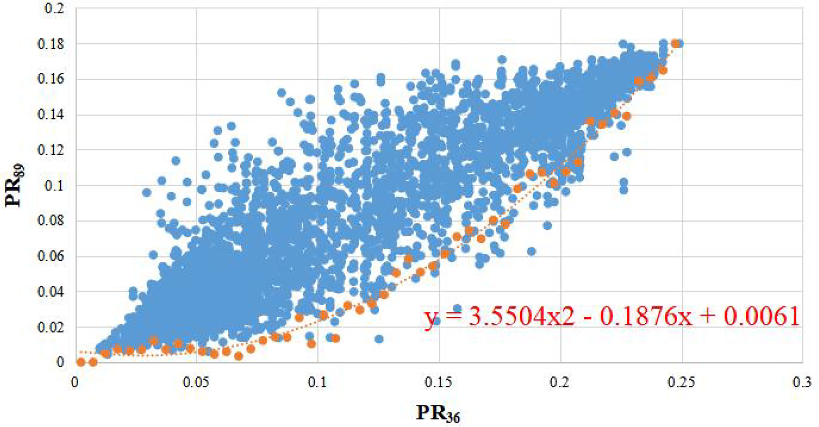
Figure 1 Scatter plot of PR.

$\begin{array}{ll}PR=\frac{T{B}_v-T{B}_H}{T{B}_v+T{B}_H}& (1)\end{array}$

Where TB_v and TB_H are the vertical polarization brightness temperature data and the horizontal polarization brightness temperature data respectively.

$\begin{array}{ll}P{R}_{89}=a*{\left(P{R}_{36}\right)}^2-b*a_{0}P{R}_{36}+c& (2)\end{array}$

Where PR₈₉ is the PR of the 89-GHz brightness temperature data and PR₃₆ is the PR of the 36-GHz brightness temperature data. And a, b, c are constants.

3.2.2 Data Correction

CGAN can better fit complex nonlinear noise data and introduce additional condition information to guide data generation, so that CGAN has better denoising effect. The generative model and the discriminative model of CGAN can get the relationship between the data affected by the external environment and the data not affected by the external environment through confrontation training. If the generative model outputs an image with poor correction results, the network parameters are continuously updated through the feedback mechanism of the discriminative model, to guide the generative model to correct the data affected by the external environment. The core idea of CGAN model is to achieve Nash equilibrium through the game (The game function of CGAN model is shown in equation (3).) between the generative model and the discriminative model. The purpose of the generative model is to generate data that is not affected by the external environment, to improve the generation ability and reduce the discrimination ability of the discriminative model. The discriminative model judges the difference of input data through the loss function, updates the parameters of CGAN model through the feedback mechanism, and finally obtains the optimal CGAN model.

$\begin{array}{ll}\begin{array}{l}{}_{\text{\hspace{0.17em}\hspace{0.17em}\hspace{0.17em}}G}^{min}{}_{\text{\hspace{0.17em}\hspace{0.17em}\hspace{0.17em}\hspace{0.17em}}D}^{max}V(G,D)=E_{x~pdata(x)}[log(D(x|y))]\\ +E_{Z~p_{z(z)}}[log(1-(D(G(z|y))))]\end{array}& (3)\end{array}$

Where x is the data affected by the external environment, y is the additional information, z is the input random noise, G (z | y) is the data that not affected by the external environment and that output by the generation network of CGAN, D (G(z | y)) is the probability that the discriminative network judges whether the input data is false. Since the goal of the generative model of CGAN is to make the generated data close to the data that not affected by the external environment as much as possible, the loss function is set to 1 - (D(G(z | y))) to ensure that the probability of judging the output false image of the discriminative network as small as possible. The goal of the discriminative model is to improve the ability to judge the difference of input data. Therefore, the larger D (x | y) is, the better it is. At the same time, the smaller the noise impacts, the better it is. The loss function is set to D (x | y) + 1 – (D(G(z | y)). Use $m{i}_G^n{m}^a{}_D^{x}V(D,G)$ to represent the process of the game.

The convolutional neural network (CNN) based on the U-Net model can integrate the characteristics of different network layers by the skip connection and improve the denoising performance, and it has strong adaptability and can effectively retain the structural information of the image. Thus, the CNN based on the U-Net model was used as the generative model in this paper, and it includes input layer, convolution layer, pooling layer, activation layer, and output layer. We set the size of the pool layer to 2 × 2, and set the size of the convolution filter to 3 × 3, and selected Rectified Linear Unit (ReLU) as the activation function.

The function of discriminative model is to distinguish two sets of relationships, that is, the relationship between the 89-GHz brightness temperature data with large interference and the 36-GHz brightness temperature data obtained by the generative model, and the relationship between the undisturbed 89-GHz brightness temperature data and the 36-GHz brightness temperature data with the high reliability. The discriminative model adopted the CNN network. Firstly, the image was input into the discriminative model, and then the batch normalization (BN) operation was performed on the input image. Secondly, the feature is extracted through convolution. Thirdly, the ReLU activation function is used for the non-linear mapping, and the final loss is calculated by cross entropy. Finally, the corrected 89-GHz brightness temperature data was obtained. So CGAN was applied to data correction as follows.

(1) Before the training, adjust the data set, such as rotation, translation, to increase the number of data set. After that, the training set and the test set are normalized.

(2) Input the training set into the generative model, and then perform continuous BN + convolution + ReLU + pooling to complete the down sampling operation.

(3) Continuous operations such as deconvolution, ReLU and dropout are performed on the feature map obtained by down sampling to complete up sampling.

(4) The output characteristic diagram of the down sampling is connected with the output characteristic diagram of the up sampling (In the same network layer, each neural network node of the current neural network layer uses the dense jump connections for the feature fusion. In different network layers, from top-layer neural network to bottom-layer neural network, the output feature maps of the down sampling and the up sampling of the next neural network layers are fused.). Then the relationship between the 89-GHz brightness temperature data and the 36-GHz brightness temperature data with the high reliability is obtained.

(5) The test set data (undisturbed 89-GHz brightness temperature data and 36-GHz brightness temperature data) and the relationship between the 89-GHz brightness temperature data obtained in the previous step and the 36-GHz brightness temperature data with the high reliability are input into the discriminative model.

(6) Carry out BN + convolution + ReLU + pooling to complete the down-sampling operation.

(7) The cross entropy is used to judge the results obtained by the discriminative model. If the loss function reaches the minimum value, the corrected 89-GHz brightness temperature data is output. Otherwise, return to step (2), and repeat the above steps until the loss function reaches the minimum value. The flowchart of the affected 89-GHz brightness temperature data correction based on CGAN model is shown in Figure 2.

FIGURE 2

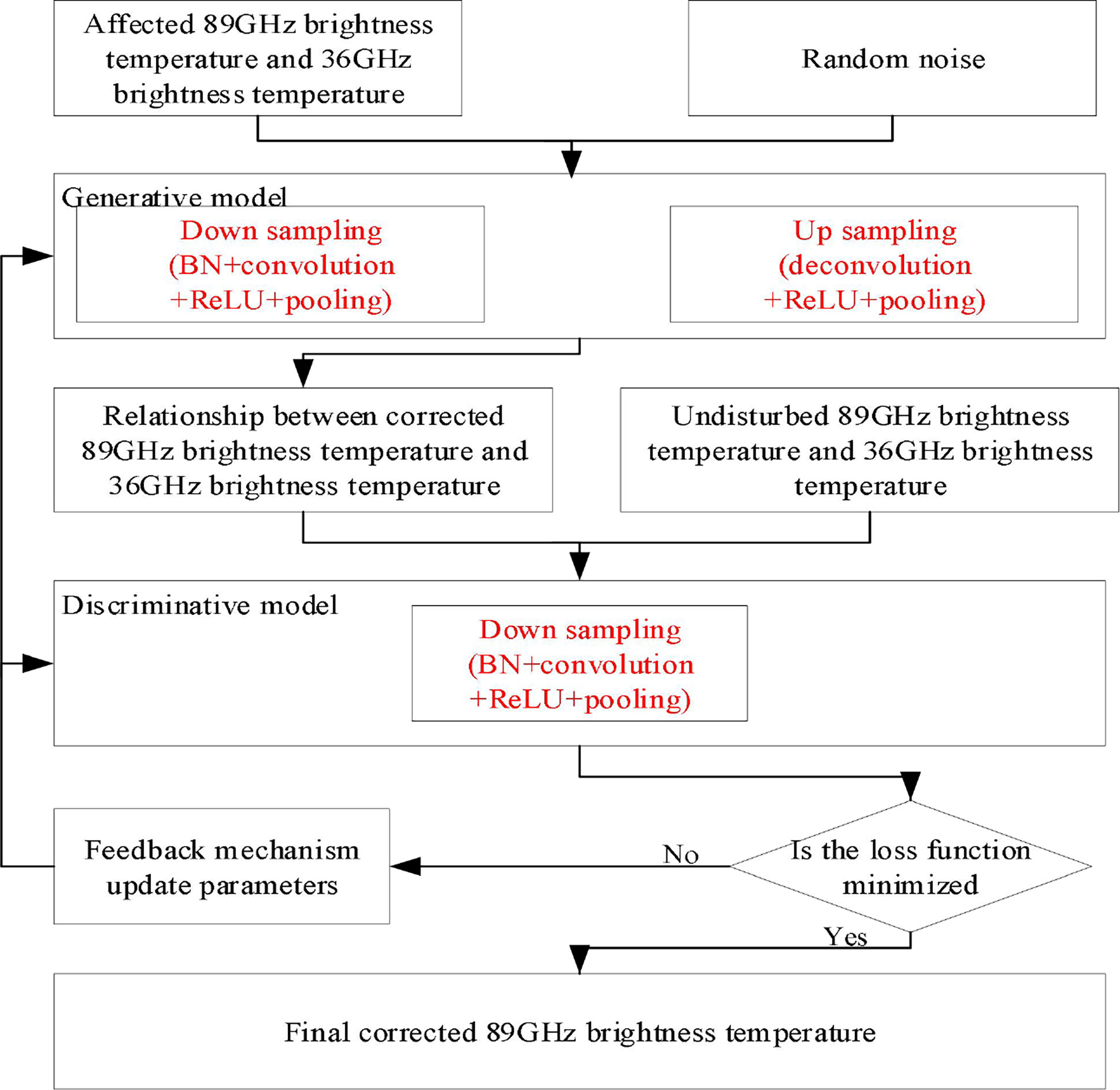
Figure 2 Flowchart of the affected 89-GHz brightness temperature data correction based on CGAN model.

4 Results and Verification

Based on the AMSR-2 89-GHz brightness temperature data, we used the ASI algorithm and the improved ASI algorithm based on CGAN to retrieve Antarctic sea ice concentration on February 1, 2021 as shown in Figure 3, and then further verified sea ice concentration by the Landsat 8 OLI-L1T data.

FIGURE 3

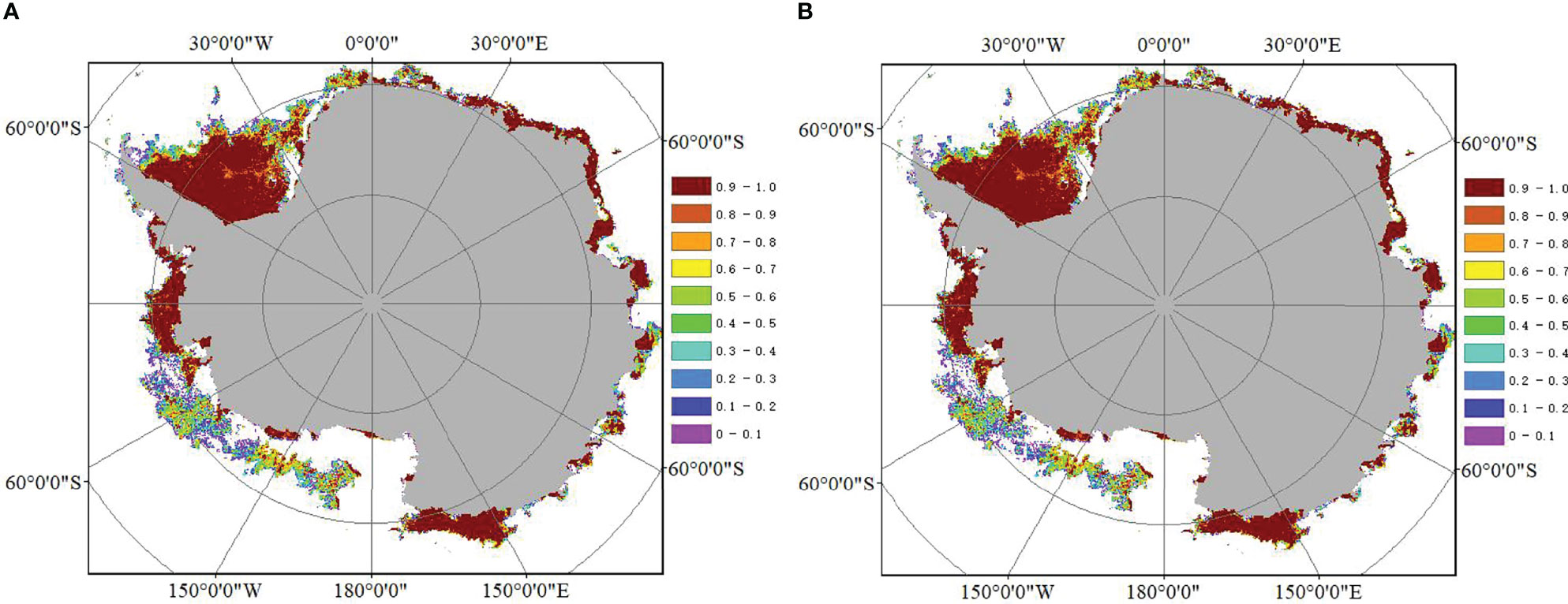
Figure 3 (A) Sea ice concentration was retrieved by the ASI algorithm; (B) Sea ice concentration was retrieved by the improved ASI algorithm based on CGAN.(Projection: polar stereographic projection) Figure 3 showed sea ice concentration retrieved by the ASI algorithm and the improved ASI algorithm based on CGAN, respectively. By comparing the results in Figure 3, it can be seen that sea ice concentration are relatively similar. Then the extents of the multi-year ice, first-year ice and total sea ice from the U.S. National Ice Center (USNIC) data, the improved ASI algorithm based on CGAN and the ASI algorithm were comared on February 1, 2021 as shown in Figure 4. It can see from Figure 4 that the sea ice extent of the improved ASI algorithm based on CGAN is between USNIC and the original ASI algorithm.

FIGURE 4

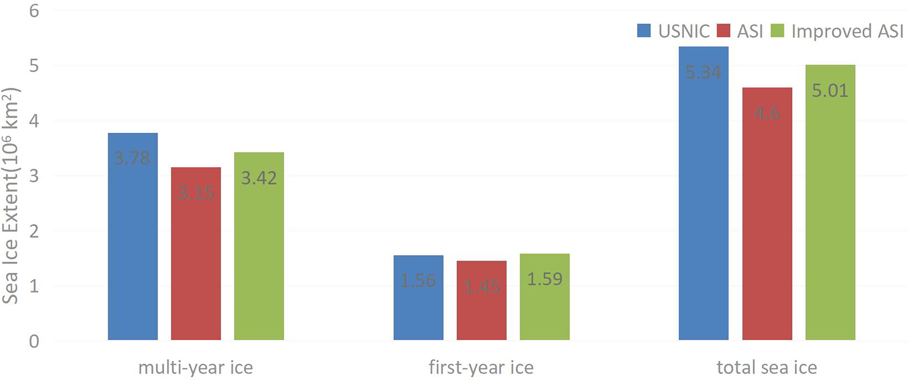
Figure 4 Comparison of Antarctic sea ice extent.

According to the Landsat 8 OLI-L1T data (resolution: 30m), we selected Landsat images for the different regions from October 2019 to March 2020 for the further verification. Based on the Landsat 8 OLI-L1T data, we used NDSI (normalized difference snow index) calculated by the near-infrared band and the short-wave near-infrared band to identify the sea ice distribution. Because this method can identifiy sea ice and sea water according to the reflectivity difference between sea ice and sea water (Perovich, 1996; Riggs et al., 1999; Hall et al., 2001; Riggs and Hall, 2015; Liu et al., 2016).

In order to further verify that the sea ice concentration retrieved by the improved ASI algorithm based on CGAN has higher accuracy than the ASI algorithm, the Landsat 8 OLI-L1T data is used to verify the results retrieved by the improved ASI algorithm based on CGAN and the ASI algorithm from. The Landsat 8 OLI-L1T data were all used under a clear sky, and the errors caused by cloud and water vapor in the processing process can be eliminated. Sea ice distribution obtained by the ASI algorithm, the improved ASI algorithm based on CGAN and the Landsat 8 OLI-L1T data shown in Figure 5A–C (February 1, 2020), Figure 5D–F (October 16, 2019), Figure 5G–I (November 10, 2019), and Figure 5J–L (March 6, 2020).

FIGURE 5

Figure 5 (A) Sea ice distribution was obtained by the ASI algorithm on February 1, 2020 (B) Sea ice distribution was obtained by the improved ASI algorithm based on CGAN on February 1, 2020 (C) Sea ice distribution was obtained by the Landsat8 OLI-L1T data through the NDSI method on February 1, 2020. (D) Sea ice distribution was obtained by the ASI algorithm on October 16, 2019 (E) Sea ice distribution was obtained by the improved ASI algorithm based on CGAN on October 16, 2019 (F) Sea ice distribution was obtained by the Landsat8 OLI-L1T data through the NDSI method on October 16, 2019. (G) Sea ice distribution was obtained by the ASI algorithm on November 10, 2019 (H) Sea ice distribution was obtained by the improved ASI algorithm based on CGAN on November 10, 2019 (I) Sea ice distribution was obtained by the Landsat8 OLI-L1T data through the NDSI method on November 10, 2019. (J) Sea ice distribution was obtained by the ASI algorithm on March 6, 2020 (K) Sea ice distribution was obtained by the improved ASI algorithm based on CGAN on March 6, 2020 (L) Sea ice distribution was obtained by the Landsat8 OLI-L1T data through the NDSI method on March 6, 2020 (Projection: polar stereographic projection; The white area is sea ice, and the black area is sea water).

In Figure 5A–C, the accuracy of the sea ice distribution obtained by the improved ASI algorithm based on CGAN is about 91%, and the accuracy of the sea ice distribution obtained by the ASI algorithm is about 83%. In Figure 5D–F, the accuracy of the sea ice distribution obtained by the improved ASI algorithm based on CGAN is 83%, and the accuracy of the sea ice distribution obtained by the ASI algorithm is about 33%. In Figure 5G–I, the accuracy of the sea ice distribution obtained by the improved ASI algorithm based on CGAN is about 83%, and the accuracy of the sea ice distribution obtained by ASI algorithm is about 50%. In Figure 5J–L, the accuracy of the sea ice distribution obtained by the improved ASI algorithm based on CGAN is about 78%, and the accuracy of the sea ice distribution obtained by ASI algorithm is about 89%. The selected areas in Figure 5 are basically located in the edge areas of Figure 3 with the low sea ice concentration or the interface between sea water and sea ice. That is to say, the accuracy of the improved ASI algorithm based on CGAN is higher than that of the ASI algorithm in the arers with the low sea ice concentration. Therefore, through the comparison of the above results, we can draw a conclusion that the improved ASI algorithm based on CGAN has higher accuracy.

5 Discussion

Sea ice concentration was retrieved by the CGAN based improved ASI retrieval algorithm based on the Landsat 8 OLI-L1T data and the AMSR-E 89-GHz brightness temperature data in this paper. Compared with the sea ice distribution obtained by the ASI algorithm, the sea ice distribution obtained by the improved ASI algorithm based on CGAN was closer to the sea ice distribution obtained from the Landsat 8 OLI-L1T data, so the improved ASI algorithm based on CGAN significantly improved the accuracy of sea ice concentration. The improved ASI algorithm based on CGAN made use of the reliable 36-GHz brightness temperature data, which greatly reduced the errors caused by the atmosphere, and the proposed method effectively corrected sea ice concentration of the pixels affected by the external environment.

At present, many scholars had studied the ASI algorithm for retrieving the sea ice concentration from the 89-GHz brightness temperature data. Although the ASI algorithm has advantages due to its higher spatial resolution, compared with the low-frequency brightness temperature data, the 89-GHz brightness temperature data are more affected by cloud and water vapor, which will lead to some errors in the edge regions of sea water and sea ice. Although some errors can be eliminated by the weather filter, the most of the errors in some regions cannot be removed. Based on the previous studies and the above reasons, we proposed the improved ASI algorithm based on CGAN. That is, we used CGAN to replace the weather filter in the ASI algorithm. The generative model of CGAN increases the utilization of the image feature information through the skip connection operation, which improves the removal of the influence of cloud and water vapor. The discriminative model can retain the image feature information and realize the non-linear mapping from the image to the image. The loss function can reduce the pixel-level loss, which can remove the influence of cloud and water vapor. The improved ASI algorithm based on CGAN can corrected the 89-GHz brightness temperature data affected by the external environment in the process of training. And the improved ASI algorithm based on CGAN greatly reduced the errors caused by the atmosphere and significantly improved the accuracy of sea ice concentration.

However, the improved ASI algorithm based on CGAN has some limitations. Firstly, in the data screening stage, the relatively stable relationship between the 89-GHz brightness temperature data which is not disturbed or less affected by the external environment and the 36-GHz brightness temperature data is limited by the sample points. Secondly, there are the time difference between the Landsat 8 OLI-L1T data and the AMSR-E/AMSR-2 data, resulting in a certain error in the inversion of sea ice concentration. Finally, using the Landsat 8 OLI-L1T data has obvious advantages in verifying local small regions, but the Landsat 8 OLI-L1T data is not very suitable for large-scale and long-time series sea ice detection. Therefore, we will strive for breakthroughs in the following two aspects in future studies. Firstly, collect more representative sample points in order to get a more accurate screening model. Secondly, find more appropriate verification data (such as on-site data) to verify the results of sea ice concentration retrieved by the improved ASI algorithm based on CGAN.

6 Conclusions

In this study, the data correction method based on CGAN was used to correct the 89-GHz brightness temperature data affected by the external environment by the relatively stable relationship between the 89-GHz brightness temperature data which is not disturbed or less affected by the external environment and the 36-GHz brightness temperature data. This method effectively corrected sea ice concentration of the pixels affected by the external environment, which greatly reduced the errors caused by the atmosphere. The sea ice concentration was verified by the Landsat 8 OLI-L1T data. Firstly, the study determined the relatively stable relationship between the 36-GHz brightness temperature data and the 89-GHz brightness temperature data that were not disturbed or less affected by external environment, and we screened out the 89-GHz brightness temperature data with the large interference. Then, the data correction method based on CGAN corrected the 89-GHz brightness temperature data which was greatly affected by the external environment such as cloud and water vapor. Finally, the ASI algorithm was used to retrieve Antarctic sea ice concentration. Sea ice concentration obtained by the improved ASI algorithm based on CGAN was compared with sea ice concentration obtained by the ASI algorithm. The results showed that sea ice concentration retrieved by the improved ASI algorithm based on CGAN was close to that obtained by the ASI algorithm. We used sea ice concentration obtained from the Landsat 8 OLI-L1T data using the NDSI method to further verify the sea ice concentration retrieved by the improved ASI algorithm based on CGAN. The improved ASI algorithm based on CGAN significantly changed the sea ice concentration of the pixels affected by the external environment, so as to reduce the impact of cloud and water vapor on high-frequency data. Compared with sea ice concentration obtained by the ASI algorithm, sea ice concentration retrieved by the improved ASI algorithm based on CGAN had higher accuracy. The sea ice distribution obtained by CGAN does not need to design features in advance. For different data products, CGAN has the strong robustness and the migration ability.

Data Availability Statement

The original contributions presented in the study are included in the article/supplementary material. Further inquiries can be directed to the corresponding author.

Author Contributions

Data curation, XW and YZ. Project administration, XW, DS, and YW. Resources, XW, YW, and SY. Software, SY. Supervision, XW and DS. Validation, XW and YZ. Writing—original draft, XW and YZ. All authors have read and agreed to the published version of the manuscript.

Funding

This research was supported by the Key Projects of Science and Technology Research of Henan Province (Grant No. 202102310334), the Key Scientific Research Project in Colleges and Universities of Henan Province of China (Grant No. 22A420004), the Cultivation Programme for Young Backbone Teachers in Henan University of Technology (Grant No. 21420070).

Conflict of Interest

The authors declare that the research was conducted in the absence of any commercial or financial relationships that could be construed as a potential conflict of interest.

Publisher’s Note

All claims expressed in this article are solely those of the authors and do not necessarily represent those of their affiliated organizations, or those of the publisher, the editors and the reviewers. Any product that may be evaluated in this article, or claim that may be made by its manufacturer, is not guaranteed or endorsed by the publisher.

Acknowledgments

We would like to acknowledge the work and efforts of the author who contributed to the manuscript.

References

Cavalieri D. J., Crawford J. P., Drinkwater M. R., Eppler D. T., Farmer L. D., Jentz R. R., et al. (1991). Aircraft Active and Passive Microwave Validation of Sea Ice Concentration From the Defense Meteorological Satellite Program Special Sensor Microwave Imager. J. Geophysic. Res. 96 (C12), 21998–22008. doi: 10.1029/91JC02335

CrossRef Full Text | Google Scholar

Cavalieri D. J., Gloersen P., Campbell W. J. (1984). Determination of Sea Ice Parameters With the NIMBUS 7 SMMR. J. Geophysical. Res. Atmospheres. 89 (D4), 5355–5369. doi: 10.1029/JD089iD04p05355

CrossRef Full Text | Google Scholar

Comiso J. C. (1986). Characteristics of Arctic Winter Sea Ice From Satellite Multispectral Microwave Observations. J. Geophysical. Res. 91 (C1), 975–994. doi: 10.1029/JC091iC01p00975

CrossRef Full Text | Google Scholar

Comiso J. C. (1995). “SSM/I Sea Ice Concentrations Using the Bootstrap Algorithm,” in NASA Reference Publication 1380 (Washington, D. C: National Aeronautics and Space Administration), ISBN: ISBN: 0-87590-263-4.

Google Scholar

Hall D. K., Riggs G. A., Salomonson V. V. (2001) Algorithm Theoretical Basis Document (ATBD) for the MODIS Snow and Sea Icemapping Algorithms[EB/OL]. Available at: https://eospso.gsfc.nasa.gov/sites/default/files/atbd/atbd_mod10.pdf.

Google Scholar

Hao G., Su J. (2015). A Study of Multiyear Ice Concentration Retrieval Algorithms Using AMSR-E Data. Acta Oceanologica. Simian. 9, 102–109. doi: 10.1007/s13131-015-0656-1

CrossRef Full Text | Google Scholar

Imaoka K., Kachi M., Fujii H., Murakami H., Hori M., Ono A., et al. (2010). Global Change Observation Mission (GCOM) for Monitoring Carbon, Water Cycles, and Climate Change. Proc. IEEE 98 (5), 717–734. doi: 10.1109/JPROC.2009.2036869

CrossRef Full Text | Google Scholar

Iwamoto K., Ohshima K. I., Tamura T., Nihashi S. (2013). Estimation of Thin Ice Thickness From AMSR-E/AMSR-2 Data in the Chukchi Sea. Int. J. Remote Sens. 34 (2), 468–489. doi: 10.1080/01431161.2012.712229

CrossRef Full Text | Google Scholar

Kaleschke L., Heygster G., Lüpkes C., Vihma T., Bochert A., Hartmann J., et al. (2001). SSM/I Sea Ice Remote Sensing for Mesoscale Ocean-Atmosphere Interaction Analysis. Can. J. Remote Sens. 27 (5), 526–537. doi: 10.1080/07038992.2001.10854892

CrossRef Full Text | Google Scholar

Kern S. (2001). A New Algorithm to Retrieve the Sea Ice Concentration Using Weather-Corrected 85 GHz SSM/I Measurements (Bremen: Dept.Physics Elect.Eng.Univ.Bremen), 1–5.

Google Scholar

Kern S. (2004). A New Method for Medium-Resolution Sea Ice Analysis Using Weather-Influence Corrected Special Sensor Microwave/Imager 85 GHz Data. Int. J. Remote Sens. 25 (21), 4555–4582. doi: 10.1080/01431160410001698898

CrossRef Full Text | Google Scholar

Kern S., Heygster G. (2001). Sea-Ice Concentration Retrieval in the Antarctic Based on the SSM/I 85.5 GHz Polarization. Ann. Glaciology. 33 (1), 109–114. doi: 10.3189/172756401781818905

CrossRef Full Text | Google Scholar

Kern S., Kaleschke L., Clausi D. A. (2003). A Comparison of Two 85-GHz SSM/I Ice Concentration Algorithms With AVHRR and ERS-2 SAR Imagery. IEEE Trans. Geosci. Remote Sens. 41 (10), 2294–2306. doi: 10.1109/TGRS.2003.817181

CrossRef Full Text | Google Scholar

Knight E. J., Kvaran G. (2014). Landsat-8 Operational Land Imager Design, Characterization and Performance. Remote Sens. 6 (11), 10286–10305. doi: 10.3390/rs61110286

CrossRef Full Text | Google Scholar

Liu Y. H., Key J., Mahoney R. (2016). Sea and Freshwater Ice Concentration From VIIRS on Suomi NPP and the Future JPSS Satellites. Remote Sens. 8 (6), 523. doi: 10.3390/rs8060523

CrossRef Full Text | Google Scholar

Liu T., Liu Y., Huang X., Wang Z. (2015). Fully Constrained Least Squares for Antarctic Sea Ice Concentration Estimation Utilizing Passive Microwave Data. Geoence. Remote Sens. Letters. IEEE 12 (11), 2291–2295. doi: 10.1109/LGRS.2015.2471849

CrossRef Full Text | Google Scholar

Lomax A. S., lubin D., Whriner R. H. (1995). The Potential for Interpreting Total and Multiyear Ice Concentrations in SSM/I 85. 5ghz Imagery. RenoteSensing. Environ. 54 (1), 13–26. doi: 10.1016/0034-4257(95)00082-c

Google Scholar

Markus T., Cavalieri D. J. (2000). An Enhancement of the NASA Team Sea Ice Algorithm. IEE. Trans. Ceoscience. Renote. Sens. 38 (3), 1387–1398. doi: 10.1109/36.843033

CrossRef Full Text | Google Scholar

Perovich D. K. (1996). The Optical Properties of Sea Ice, CRREL Monogr. No. 96-1. U.S. Army Cold Regions Research and Engi-Neering Laboratory. 25.

Google Scholar

Riggs G. A., Hall D. K. (2015) MODIS Sea Ice Products User Guide to Collection 6[EB/OL]. Available at: https://landweb.modaps.eos-dis.nasa.gov/QA_WWW/forPage/user_guide/MODISC6SeaIce-productsUserguide.pdf.

Google Scholar

Riggs G. A., Hall D. K., Ackerman S. A. (1999). Sea Ice Extent and Classification Mapping With the Moderate Resolution Imaging Spectro-Radiometer Airborne Simulator. Remote Sens. Environ. 68 (2), 152–163. doi: 10.1016/S0034-4257(98)00107-2

CrossRef Full Text | Google Scholar

Spencer R. W., Goodman H. M., Hood R. E. (1989). Precipitation Retrieval Over Land and Ocean With SSM/I: Identification and Characteristics of the Scattering Signal. J. Atmospheric. Oceanic. Technol. 6, 254–273. doi: 10.1175/1520-0426(1989)006<0254:PROLAO>2.0.CO;2

CrossRef Full Text | Google Scholar

Spreen G., Kaleschke L., Heygster G. (2008). Sea Ice Remote Sensing Using AMSR-E 89-GHz Channels. J. Geophysical. Res. Atmospheres. 113 (113), C02S03. doi: 10.1029/2005JC003384

CrossRef Full Text | Google Scholar

Su J., Hao G. H., Ye X. X., Wang W. B. (2013). The Experiment and Validation of Sea Ice Concentration AMSR-E Retrieval Algorithm in Polar Region. J. Remote Sens. 17 (3), 495–513. doi: CNKI:SUN:YGXB.0.2013-03-005

Google Scholar

Svendsen E., Mauler C., Grenfell T. C. (1987). A Model for Retrieving Total Sea Ice Concentration From a Spaceborne Dual-Polarization Passive Microwave Instrument Operating Near 90ghz. Int. J. Remote Sens. 8 (10), 1479–1487. doi: 10.1080/01431168708954790

CrossRef Full Text | Google Scholar

Wang, H. (2009). Multiyear Ice Retrieval Using Passive Microwave Remote Sensing Radiometer AMSR-E 89ghz Data (in Chinese) (Qingdao: Ocean University of China).

Google Scholar

Wu Z., Wang X., Wang X. (2019). An Improved ARTSIST Sea Ice Algorithm Based on 19 GHz Modified 91 GHz. Acta Oceanologica. Sin. 38 (10), 93–99. doi: 10.1007/s13131-019-1482-7

CrossRef Full Text | Google Scholar

Zhang, S. (2012). Sea Ice Concentration Algorithm and Study on the Physical Process About Sea Ice and Melt-Pond Change in Central Arctic (in Chinese) (Qingdao: Ocean University of China).

Google Scholar