The Ups and Downs of Using Active Acoustic Technologies to Study Fish at Tidal Energy Sites

1 Introduction

The tidal energy sector is a nascent industry, and the potential environmental effects of marine hydrokinetic (MHK) devices on fish continues to be an area of concern for regulators and stakeholders of the marine environment (Copping et al., 2021). Predicting fish interactions with MHK devices, and therefore potential device effects, requires information on fish presence, abundance, and distribution at a resolution and scale that is rarely required elsewhere. Spatial resolution must be on the order of meters for data to be related to an individual MHK device, and collected throughout the water column and/or across tidal channels that can be kilometers wide. Similarly, fine temporal resolution (seconds to minutes) may be required to capture shifts in fish distribution that affect MHK device encounter rates but years of observations may be needed to characterize seasonal patterns and longer-term population shifts. Active acoustic instruments are excellent tools for collecting this high-resolution information across large spaces and periods of time. This technology includes single beam, split beam, and multibeam echosounders utilizing single or multiple frequencies in narrow- or broad-band modes (Demer et al., 2015). Active acoustics is a vital component of fisheries stock assessments worldwide, given these instruments’ unequaled capacity to rapidly and non-invasively sample large volumes of water (Horne, 2000; Simmonds and MacLennan, 2005). Echosounders have been employed in studies of fish at tidal energy sites around the world, as well (e.g. Viehman et al., 2015; Fraser et al., 2017; Viehman et al., 2018; Gonzalez et al., 2019; Williamson et al., 2019; Scherelis et al., 2020; Whitton et al., 2020).

Tidal channels are characterized by fast currents and complex hydrodynamics that pose unique challenges to active acoustics technology, which can hamper the translation of raw data to information that can be used by scientists, developers, and regulators of the tidal energy industry. The primary challenge is the high prevalence of air bubbles entrained into the water column, which scatter the sound transmitted by echosounders. Air entrainment is a common occurrence in the open ocean, with the primary source of entrainment being breaking waves (Woolf, 2001; Baschek et al., 2006). Air plumes in the open ocean commonly extend to depths of 10-15 m, but the extreme hydrodynamic conditions in areas with strong tidal currents can draw bubbles to depths well over 100 m (Baschek et al., 2006). Though bubbles entrained in the water column tend to be very small (e.g. < 1 mm diameter; Woolf, 2001; Baschek et al., 2006), they are strong scatterers of sound. The sound scattered by clouds of bubbles observed at tidal energy sites is similar to, or stronger than, that scattered by fish (for example, in the 120 kHz data assessed here, volume backscatter of the entrained air layer averaged -46 dB re 1 m²m^-3), and the two scatterer types cannot be separated in active acoustics data if they inhabit the same volume of water. Measurements containing backscatter from entrained air must therefore be removed from acoustic datasets prior to analyzing backscatter from fish.

Studies at tidal energy sites have utilized different methods to remove backscatter from entrained air. The majority of methods exploit the distinct temporal and/or morphological characteristics of the bubble plumes to differentiate them from fish backscatter, including occurrence and duration in time and surface connectivity (Fraser et al., 2017; Scherelis et al., 2020). Features with the designated characteristics are then removed from the dataset, either manually or with some mix of automated and manual steps. Removal has included omitting just the contaminated data points (Fraser et al., 2017; Whitton et al., 2020), or a fixed depth range plus the entire water column when air extends further (Viehman et al., 2018). Other studies have kept only the lowermost portion of the water column as the depths of primary interest, ignoring the upper layers (Viehman et al., 2015; Gonzalez et al., 2019). Regardless of the method, the result is omitting a large amount of water that could contain fish but is unable to be effectively sampled by active acoustics instruments.

Omitting the entrained air layer is likely to affect acoustically derived estimates of fish abundance and vertical distribution, and therefore our ability to estimate encounters with MHK devices. Moreover, it is possible that different fish species’ or life stages’ contributions to acoustic measurements will be unequally affected by removing different portions of the water column, given depth preferences that are often species- or life-stage-specific. For example, in the northwest Atlantic, Atlantic salmon post-smolts and adults (Salmo salar) tend to be found within the upper 10 m of the water column (Dutil and Coutu, 1988; Sheehan et al., 2012). Other species utilize the entire water column more generally (e.g. Atlantic herring, Clupea harengus, Huse et al., 2012; Viehman et al., 2018; Atlantic mackerel, Scombur scombrus, Castonguay and Gilbert 1995), while others are typically associated with the bottom (e.g. Atlantic cod, Gadus morhua, Hobson et al., 2007). American eel (Anguila rostrata) have exhibited distinct vertical migrations to take advantage of favorable tidal currents, a behavior known as selective tidal stream transport (STST; Parker and McCleave, 1997). At present, it is unclear whether depth preferences observed in lower-energy environments will persist within highly energetic tidal channels, and there is some evidence that they may differ (Stokesbury et al., 2016; Lilly et al., 2021).

Though data contamination by entrained air is an issue at all tidal energy sites, we have yet to examine the resulting data loss in detail (e.g. its magnitude and spatiotemporal distribution), or how this loss could affect our acoustically derived estimates of fish abundance and vertical distribution. This information would be particularly helpful in the planning stages of a study or environmental monitoring plan, when steps can be taken to address any expected limitations of the active acoustic dataset. These steps may include, for example, the simultaneous use of complementary technologies and sampling techniques.

In this paper, we examined the entrained air layer in active acoustic data collected at the FORCE tidal energy test site. We developed a method for identifying and removing the data points contaminated by entrained air, quantified entrained air depth and resulting data loss, and demonstrated the effects of this data loss on estimates of fish abundance and vertical distribution obtained from simulated vertical distributions of fish. The active acoustic data assessed in this paper are from a fixed-location split beam, narrowband, scientific-grade echosounder, which is the type most used for assessing the abundance and vertical distribution of fishes over long periods of time or space. Our goal was to provide researchers, developers, and regulators of the tidal energy industry with the information they need to utilize active acoustics technology to its fullest potential, and to mitigate the limitations imposed on it by this exceptionally challenging environment.

2 Materials And Methods

2.1 Data Collection

Data were collected at the Fundy Ocean Research Center for Energy (FORCE) tidal energy test site, in the Bay of Fundy, Nova Scotia, Canada (Figure 1). Instruments were installed on the Fundy Advanced Sensor Technology subsea platform, FAST-3 (Figure 2). This stationary platform was deployed on the seafloor at 45°21’47.34” N, 64°25’38.88” W, and was in place for 53 days from 30 March to 23 May 2018. At this location, water column depth averaged 33 m at low tide and 43 m at high tide.

FIGURE 1

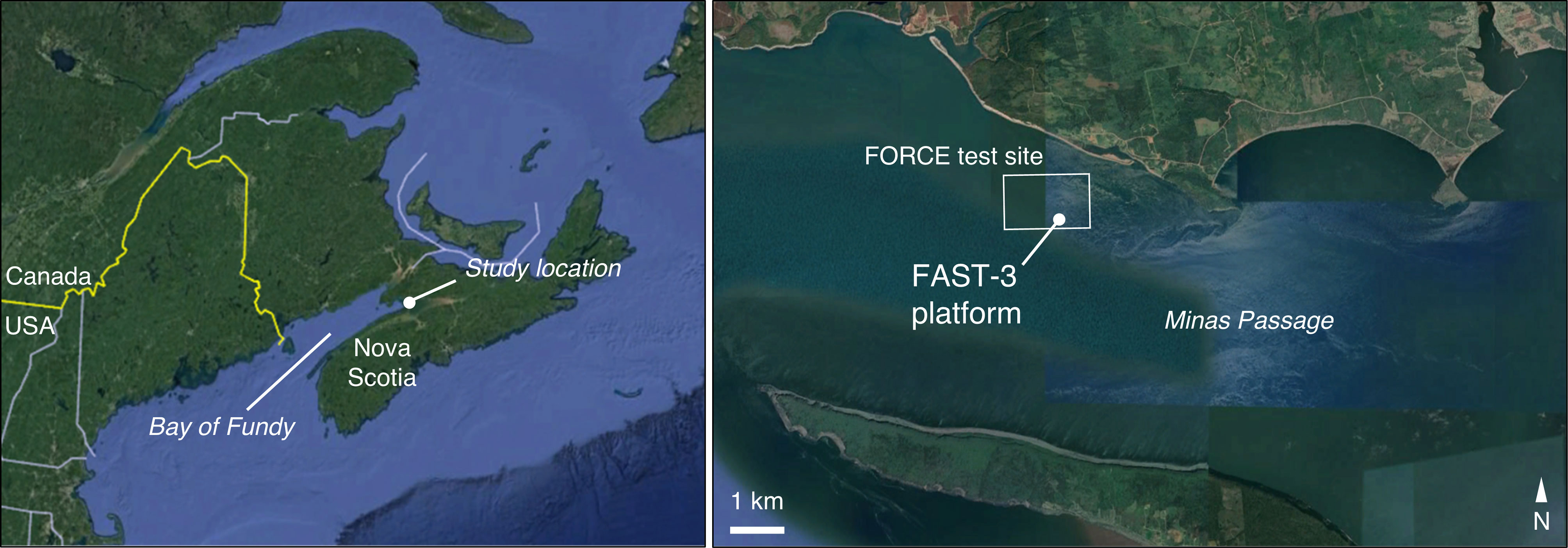
Figure 1 Study location in the Minas Passage of the Bay of Fundy, Canada. The location of Minas Passage is indicated by the filled circle in the left-hand panel, and the study site is shown on the right.

FIGURE 2

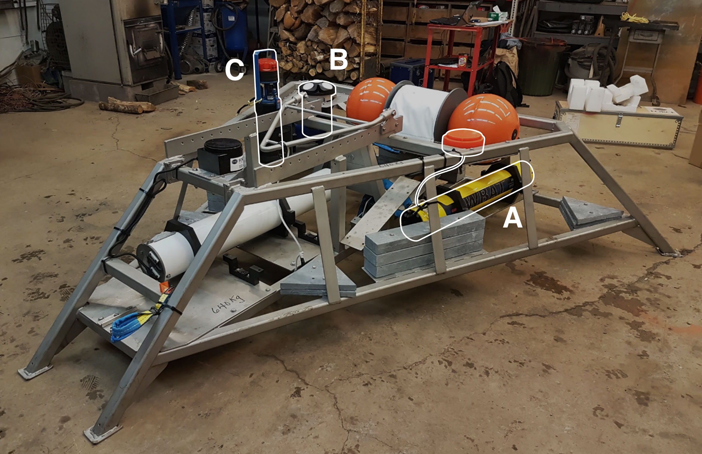
Figure 2 FAST-3 platform deployed at the FORCE Tidal energy test site from 30 Mar to 23 May 2018. Equipment included (A) Simrad WBAT EK80 echosounder, (B) Nortek Signature 500 ADCP, (C) Aanderaa SeaGuard RCM.

Active acoustic data were collected by a Simrad EK80 WBAT echosounder with a 120 kHz split beam transducer (7° half-power beam angle), located 0.7 m above the seafloor and facing upward. Data were collected in 5-min recording periods every half hour, with a ping rate of 1 Hz, pulse duration of 0.128 ms, transmit power of 125 W, and maximum recording range of 60 m. Collection settings were chosen based on pilot data collected near this site in February 2017.

Measurements of current velocity throughout the water column were collected by a Nortek Signature 500 acoustic doppler current profiler (ADCP). The ADCP’s face was located at 0.7 m above the seafloor. Data were collected in 5-min bursts every 15 min, alternating with echosounder measurements to avoid acoustic interference between the two instruments. The sample rate during each burst was 2 Hz, the blanking distance was 1 m, and the cell size was 1 m.

Water temperature and salinity at the platform were measured by an Aanderaa SeaGuard RCM every half hour.

2.2 Data Processing

2.2.1 Active Acoustic Data

Active acoustic data processing was carried out using Echoview^® software (12.1, Myriax, Hobart, Australia). We developed a data processing routine in Echoview that detected the surface and entrained air layer, minimizing the need for manual correction as much as possible. The template developed for this process is provided in supplementary materials with a detailed explanation of all steps.

Briefly, the surface was detected with a line, and the boundary of the surface dead zone was delineated below this (0.16 m below on average; Ona and Mitson, 1996). A line was also defined at 2x the acoustic nearfield distance from the transducer face (Simmonds and MacLennan, 2005), and acted as the lower analysis limit in all following steps. Entrained air was defined morphometrically as clusters of backscatter which extended downward from the surface, similar to Fraser et al. (2017). Detection of these clusters required a series of separate processing steps, including smoothing the raw volume backscatter (S_V) data, applying a minimum data threshold, and using Echoview’s schools detection algorithm to detect contiguous clusters of backscatter that surpassed this threshold. Clusters which were connected to the surface were isolated and expanded in depth and time, and a line was drawn below the resulting backscatter to establish the lower extent of the entrained air layer. The maximum depth of this layer was limited by the acoustic nearfield, 2.4 m above the seafloor.

All processing steps and settings were chosen by iteratively reviewing the performance of the processing routine on a subset of data files that represented a wide range of entrained air contamination, until the level of necessary manual corrections to the surface and entrained air lines was deemed acceptably low. All data files were then batch-processed in Echoview using the finalized routine. The resulting Echoview files were reviewed manually to make any necessary corrections to the surface and entrained air lines.

Once all necessary corrections were made, the surface and entrained air line depths were exported, and we calculated the average water column depth and entrained air depth for each 5-min data recording period. For each recording period, we also calculated the number of samples (individual datapoints) omitted due to the entrained air layer. We converted this number to a percent of analyzable samples, which was more comparable over time as water level changed. We defined analyzable samples as all samples between the nearfield and surface dead zone because samples outside of these boundaries would always be excluded from acoustic analysis.

Echosounder data were calibrated using calibration sphere measurements obtained at a calm location off-site, before and after the deployment. As environmental conditions changed significantly over the course of the deployment (temperature and salinity shifts caused the speed of sound to increase from 1452 m·s^-1 to 1477 m·s^-1), acoustic data were split into sections to which different calibration parameters were applied. Details of data calibration are supplied in supplementary materials.

2.2.2 ADCP Data

ADCP measurements were first corrected for platform tilt and compass declination using Ocean Contour (version 2.1.5, Ocean Illumination Ltd., Canada). We obtained average horizontal speed and direction for each 1-m cell of every ADCP burst. The first measurement cell was centered 2 m from the transducer face. Measurements from the uppermost 10% of the water column could not be used due to interference from side lobes, so we removed these upper cells prior to calculating water column average speed and direction. We then interpolated these speed and direction values in time to obtain water column averages at the midpoint of each echosounder recording period. All future references to current speed or direction measurements refer to these interpolated water column averages.

Slack tide was defined as current speed < 0.5 m·s^-1, which captured the period of time when current direction was shifting between ebb and flood. In this dataset, slack tide defined in this way (by current speed and direction) occurred approximately 15-30 min after the time of lowest or highest water. Spring and neap tides were identified in the current velocity time series as maxima and minima in peak flow speed.

2.2.3 SeaGuard RCM Data

Conductivity and temperature readings from the SeaGuard RCM were used in the calculation of sound speed, for calibrating echosounder data (see supplementary material).

2.3 Data Analysis

There was no way to predict how many fish were omitted from the acoustic dataset by removing the entrained air layer. We therefore demonstrated how entrained air contamination affects estimates of fish abundance and distribution by constructing five hypothetical fish distribution scenarios that we then subjected to different levels of contamination and data removal. Analysis was carried out in R software version 4.1.2 (R Core Team, 2021).

The five vertical distribution scenarios each spanned one tidal cycle, which was split into 24 equally spaced time segments (tide bins; approximately 30 min each). All recording periods from the acoustic dataset were partitioned into these tide bins, and for each tide bin we calculated mean water column depth and the 5^th, 50^th (median), and 95^th percentiles of entrained air depth. The mean water column depth from each tide bin defined the hypothetical water column in each fish distribution scenario. The water column was then split into 1 m depth bins to be populated with some number of fish. For simplicity, total fish abundance was held constant over time (1000 fish per tide bin, 24000 fish total). The fish distribution scenarios we generated were:

1. Fish utilizing the entire water column: for each tide bin, 1000 fish were distributed randomly into all water column bins, from the seafloor to the surface.

2. Surface-oriented fish: for each tide bin, 1000 fish were distributed into the upper 10 bins of the water column. To simulate a gradual increase in fish abundance towards the surface (as observed previously; e.g. Viehman et al., 2018), fish were assigned to depth bins following a beta distribution which peaked in the 2-3 m depth bins.

3. Bottom-oriented fish: for each tide bin, 1000 fish were assigned to the lowermost 10 m of the water column, using the same method as for Scenario 2 but with fish abundance increasing towards the sea floor and peaking in the lowermost bin.

4. Selective tidal stream transport (STST): fish were bottom-oriented during the flood tide (as in Scenario 3) and surface-oriented during ebb tide (as in Scenario 2), transitioning through the mid-water-column during slack tides. This scenario represented STST for a species migrating outward toward the open ocean, utilizing the current during ebb tide.

5. Mixed fish assemblage: Scenarios 1-4 were combined to represent a mix of species exhibiting different depth preferences and vertical movements. 50% of fish were randomly distributed, 20% were surface-oriented, 20% were bottom-oriented, and 10% exhibited STST. The proportions of fish exhibiting each vertical distribution were chosen arbitrarily for illustration purposes, as these proportions are not yet known for fishes utilizing Minas Passage.

To simulate the effects of entrained air contamination on acoustically-derived estimates of fish abundance, we removed counts from any depth bins within the entrained air layer. The 5^th, 50^th, and 95^th percentile air layer depths represented “best”, “middle”, and “worst” contamination conditions, respectively. We also omitted fish below the nearfield range, as that portion of active acoustic data would not be useable either. We calculated “observed” fish abundances as the water column sums for each tide bin in these reduced datasets (making the assumption that all fish would be equally detectable by the echosounder). We then compared observed abundances to the known water column sums (“actual” fish abundance), which was 1000 fish per tide bin.

For scenario 5, we also compared actual and observed fish vertical distribution for each stage of the tide: low (tide bins 1 and 24), high (tide bin 13), flood (tide bins 2 to 12), and ebb (tide bins 14 to 23). The vertical distribution for each tidal stage was constructed by breaking the water column into depth bins which spanned 5% of the total water column height (to account for changing water level), then summing the numbers of fish contained within each percentage bin.

3 Results

The entrained air detection method worked well, with only a small number of files requiring manual adjustments to the automatically detected surface and entrained air lines (approximately 6% and 3%, respectively). Most entrained air was easily identifiable as backscatter extending downward from the surface, whereas most backscatter likely to be from fish did not overlap with the surface (Figure 3).

FIGURE 3

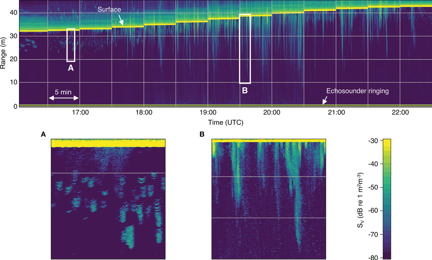
Figure 3 Volume backscatter (S_V) echogram from a typical flood tide (on 22 May 2018). Low tide is on the left and high tide is on the right. Vertical gridlines separate the 5-min echosounder recording periods, which began every half hour (times shown in UTC). Horizontal gridlines indicate 10-m range bins (measured upwards from the transducer face). All following echograms use the same grid and color scale shown here. (A) Backscatter from small aggregations of fish visible near the surface near low tide. (B) Bubble plumes extending far into the water column during the peak flow.

Despite the entrained air layer detection algorithm generally working well (Figure 4A), there were still instances where it was difficult to differentiate backscatter from bubbles or fish based on appearance alone. Some backscatter could have been either aggregated fish or partial, detached bubble plumes (Figure 4C). This ambiguous backscatter needed to be classified manually based on the appearance of the surrounding water column and neighboring recording periods. There were also many periods where fish were evident within bubble plumes but inseparable from plume backscatter, and therefore omitted (Figure 4B).

FIGURE 4

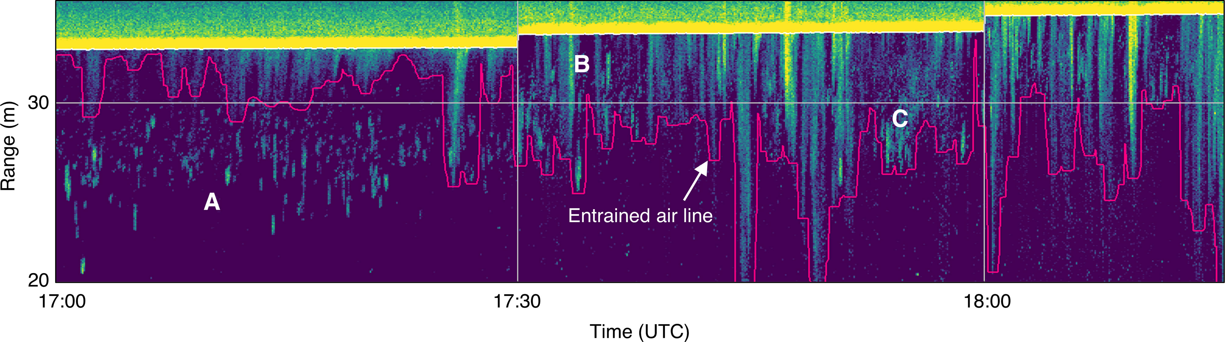
Figure 4 Subset of echogram shown in (Figure 3), showing backscatter from fish and entrained air (delineated by pink line). (A) Small fish aggregations clearly visible in upper water column, separate from entrained air layer. (B) Aggregations appear to shift upward into entrained air layer, where they can still be seen. (C) Unclear whether backscatter is from fish aggregations or detached/dispersed bubble plumes.

Backscatter from entrained air was not always confined to dense plumes of bubbles. At peak current speeds, when the plumes were most obvious, it was clear that the remaining water column was also subject to additional backscatter that often surpassed the same minimum threshold applied to the plumes (Figure 5). This more dispersed backscatter was likely also related to bubbles, given its strong association with deep bubble plumes, and it was therefore considered to be part of the entrained air layer. This situation is the cause of all recording periods that were missing 100% of their analyzable samples.

FIGURE 5

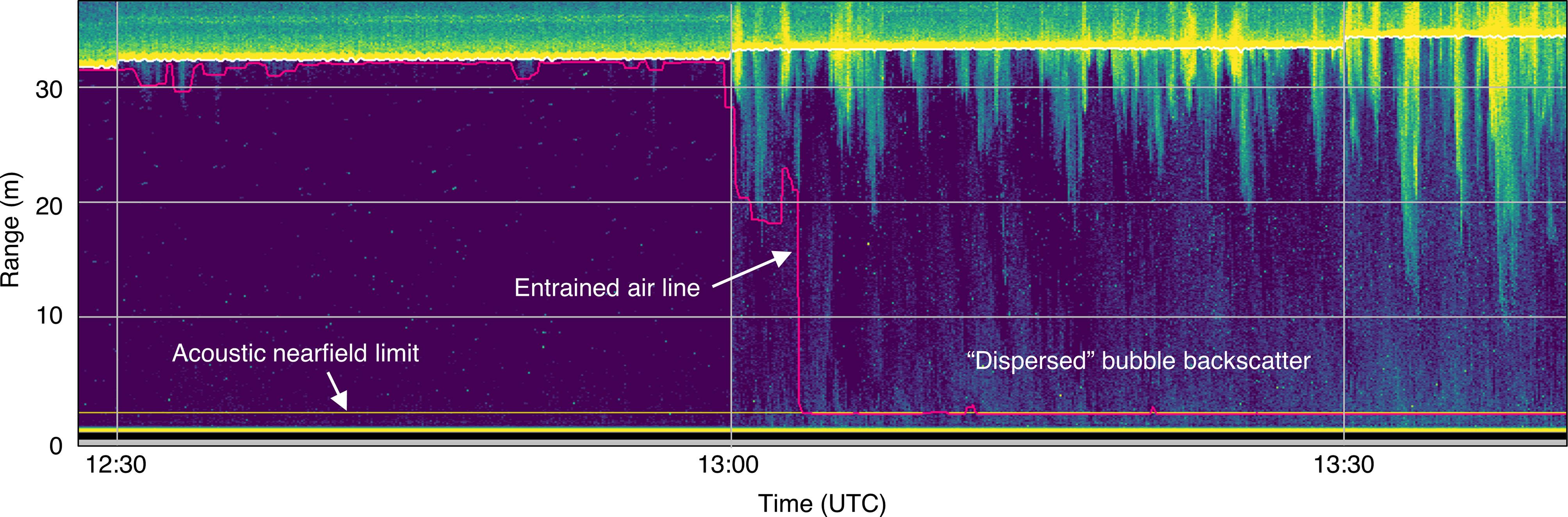
Figure 5 Example of backscatter from bubbles entrained throughout the water column. The detected entrained air line (pink) extends to the acoustic nearfield (horizontal yellow line), resulting in omission of most or all of the water column.

The final dataset consisted of 2583 5-min recording periods. Across all recording periods, 29% of all analyzable samples were removed due to contamination from entrained air. Entrained air depth varied greatly over time, from the surface to the nearfield-exclusion line (Figure 6B). Consequently, the percentage of analyzable samples that would be omitted from any given recording period also varied from near 0% up to 100% (Figure 6C). Overall, 4% of recording periods were missing all of their analyzable samples, 16% were missing at least half of their samples, and 41% were missing at least a quarter. Almost all recording periods missing 100% of their samples occurred during peak flow near spring tides, when current speeds were highest (Figures 6A, C, orange bars). During neap tides, data loss in a given recording period did not often exceed 50% (Figure 6C, purple bars).

FIGURE 6

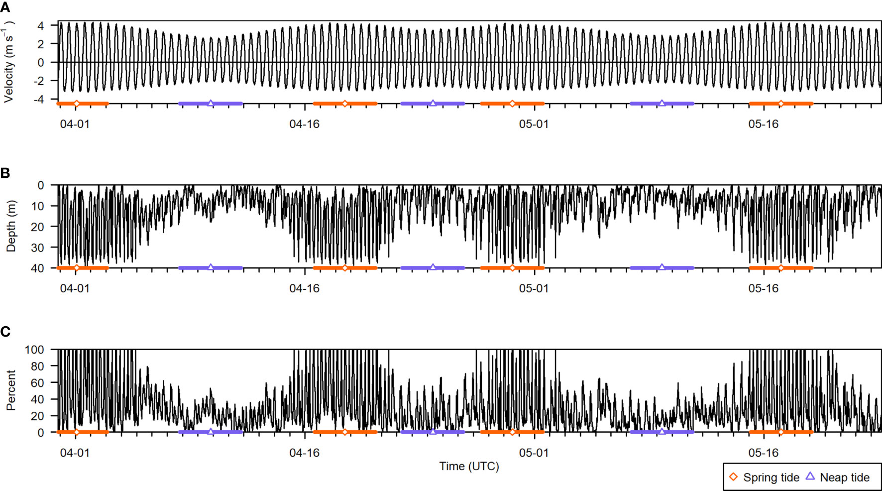
Figure 6 Summary of all active acoustic recording periods from the deployment, spanning 30 March to 23 May 2018. (A) Current velocity (negative is ebb direction, positive is flood), (B) entrained air depth, and (C) percent of analyzable samples that were contaminated by entrained air in each recording period. The times of spring and neap tides are indicated by the orange diamond and purple triangle symbols, respectively, and the colored bars span 2 days on either side. Note that the entrained air layer depth stops at the acoustic nearfield, located 2.4 m above the seafloor.

Due to entrained air extending downward from the surface, the lower water column was sampled more consistently than the upper water column. Across all recording periods, the uppermost 5% of the water column was only sampled 15% of the time, whereas the 5% above the nearfield was sampled 93% of the time (Figure 7A). The uppermost water column was almost exclusively sampled at current speeds less than 2 m·s^-1, and current speeds over 3 m·s^-1 were only well sampled in the lower half of the water column (i.e. in proportions similar to total recording periods, Figure 7A, upper panel). The fastest current speeds, greater than 4 m·s^-1, were very rarely sampled without contamination from entrained air, and only in the lower 45% of the water column.

FIGURE 7

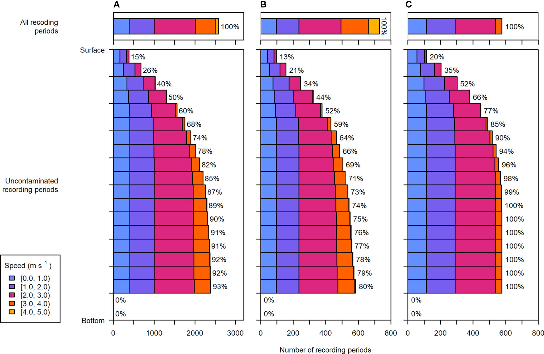
Figure 7 Distribution of depths and current speeds sampled during (A) the entire dataset, (B) recording periods within 2 days of spring tides, and (C) recording periods within 2 days of neap tides. Upper panels: the current speeds recorded during all periods of the respective data subset, representing speeds that would be sampled throughout the water column if there were no contamination from entrained air. Lower panels: the depth and current speed distribution of uncontaminated recording periods. Each depth bin spans 5% of the water column (the lowermost two depth bins were not sampled in any recording periods due to the height of the nearfield exclusion above the sea floor). To the right of each bar is the percentage of total recording periods within the respective data subset (e.g., entire dataset, spring tide, or neap tide).

There was a noticeable difference between depths and current speeds sampled during spring and neap tides (Figures 7B, C). Most current speeds greater than 3 m·s^-1 occurred during spring tides (Figure 7B, upper panel), but were not well sampled anywhere in the water column (Figure 7B, lower panel). During spring tide, contamination by entrained air at these faster speeds resulted in omitting at least 20% of recording periods throughout the water column, and more closer to the surface.

Conversely, during neap tides, the current speeds sampled in the lowermost 75% of the water column largely reflected the current speeds measured across all neap tide periods. Moreover, bins in the lower 70% of the water column were contaminated less than 10% of the time. Though surface depth bins were still under-sampled relative to lower bins, data collected during neap tides spanned the most representative range of current speeds for the largest portion of the water column.

The unequal representation of current speeds across depths was due to the correlation of entrained air depth with current speed (Figure 8A). Higher current speeds resulted in greater air contamination and data loss. The highest current speeds recorded during either flood or ebb tide (occurring near spring tides) were often correlated with 100% contaminated samples (Figure 8B), though peak speeds were lower during ebb than flood (Figure 9C). The recording periods missing all or nearly all samples were mainly due to the “dispersed” bubble backscatter shown in Figure 5.

FIGURE 8

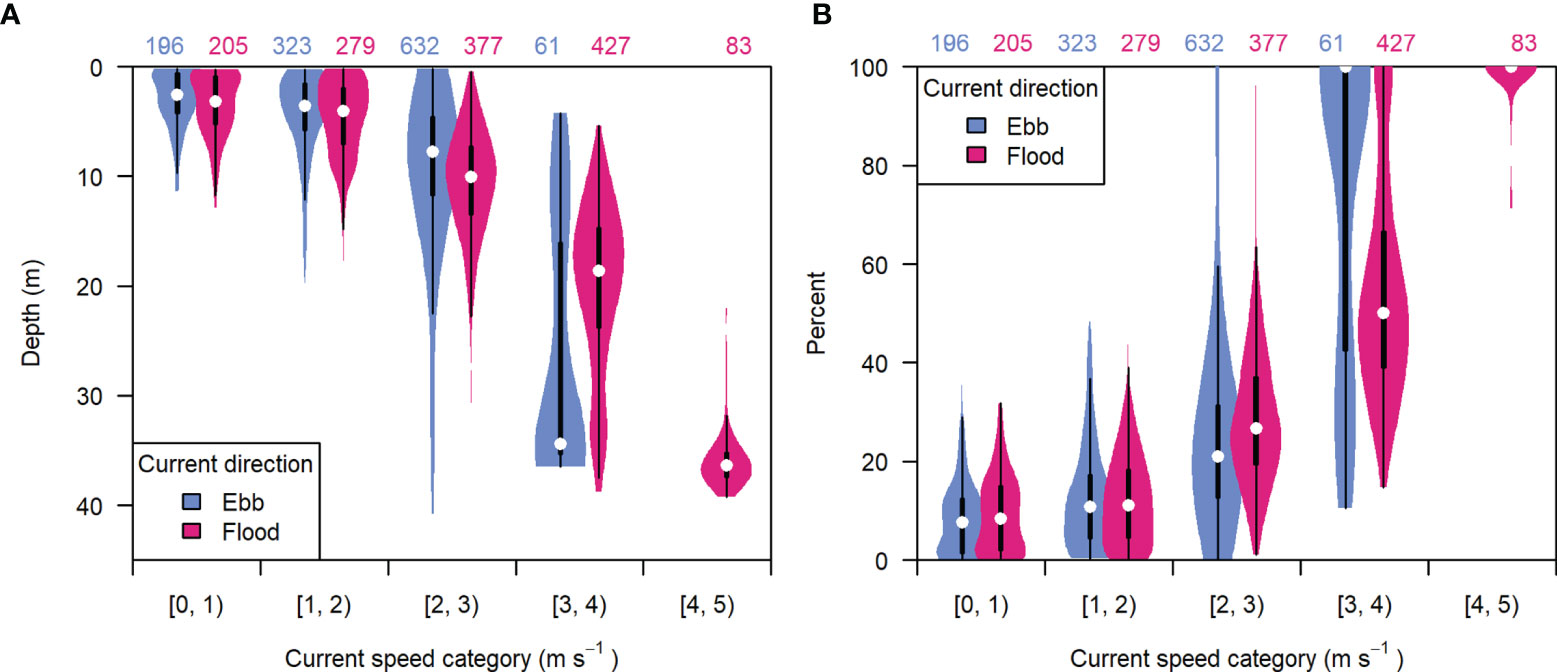
Figure 8 The distribution of (A) entrained air depth and (B) percent of analyzable samples missing from each recording period, grouped by current speed category and tidal current direction (ebb or flood). Light blue indicates ebb tide, dark pink indicates flood tide. White points are the median value, boxes span the interquartile range (IQR), whiskers extend to 1.5*IQR, and violins span the minimum and maximum values in each group. Numbers at the top indicate the number of recording periods in each group.

The correlation of entrained air depth with current speed meant the uncontaminated portion of the water column grew and shrank in an approximately 6-hour cycle, aligned with the tidal currents. This was very clear when data were summarized by tide bin (Figure 9).

FIGURE 9

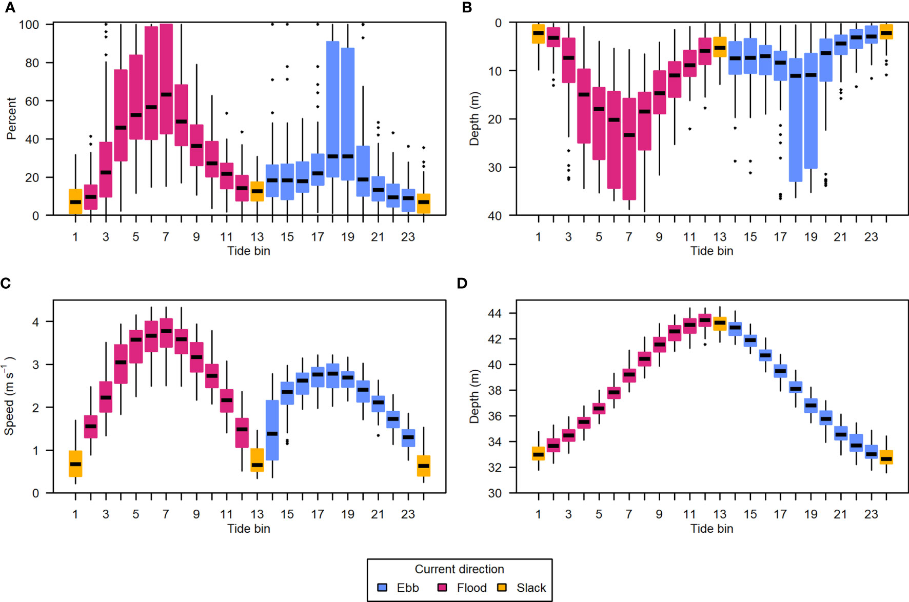
Figure 9 Data from all recording periods summarized by position in the tidal cycle. (A) Percent of analyzable samples missing due to entrained air contamination, (B) depth of entrained air layer relative to the surface, (C) water column mean current speed, and (D) water column total depth. The tidal cycle was divided into 24 equal bins, each spanning approximately half an hour. Light blue indicates ebb tide, dark pink indicates flood tide, and yellow indicates the tide bins containing slack tides. Horizontal black lines are the median of each group, boxes span the interquartile range (IQR), whiskers extend to 1.5*IQR, and points are outlying values.

The 5 hypothetical fish distribution scenarios are shown in Figures 10A–E, along with samples removed according to the 5^th, 50^th, and 95^th percentile entrained air depth for each tide bin (hatchlines), and acoustic nearfield (crosshatched area along the bottom). Different levels of entrained air contamination had clear effects on fish abundances obtained from each of the 5 distribution scenarios (Figure 11). The magnitude of the impact on “observed” fish abundance over the course of the tidal cycle varied according to the underlying vertical distribution of fish. Generally, error in abundance estimates was greatest whenever fish were most concentrated in the upper water column (Figures 11B, D). For scenarios with fish in the upper- and mid-water-column, omission of data in the entrained air layer generated a distinct tidal pattern in observed fish abundance, as fewer fish were detected at higher current speeds (Figures 11A, B, D, E). This was true for all three entrained air levels applied to the simulated scenarios. Observed abundance of fish inhabiting the lowermost water column was primarily affected by the exclusion of data in the acoustic nearfield (a constant negative bias; Figure 11C, solid red line); however, lower-water-column observed abundances were also affected by the more extreme level of entrained air contamination (Figure 11C, dashed red line).

FIGURE 10

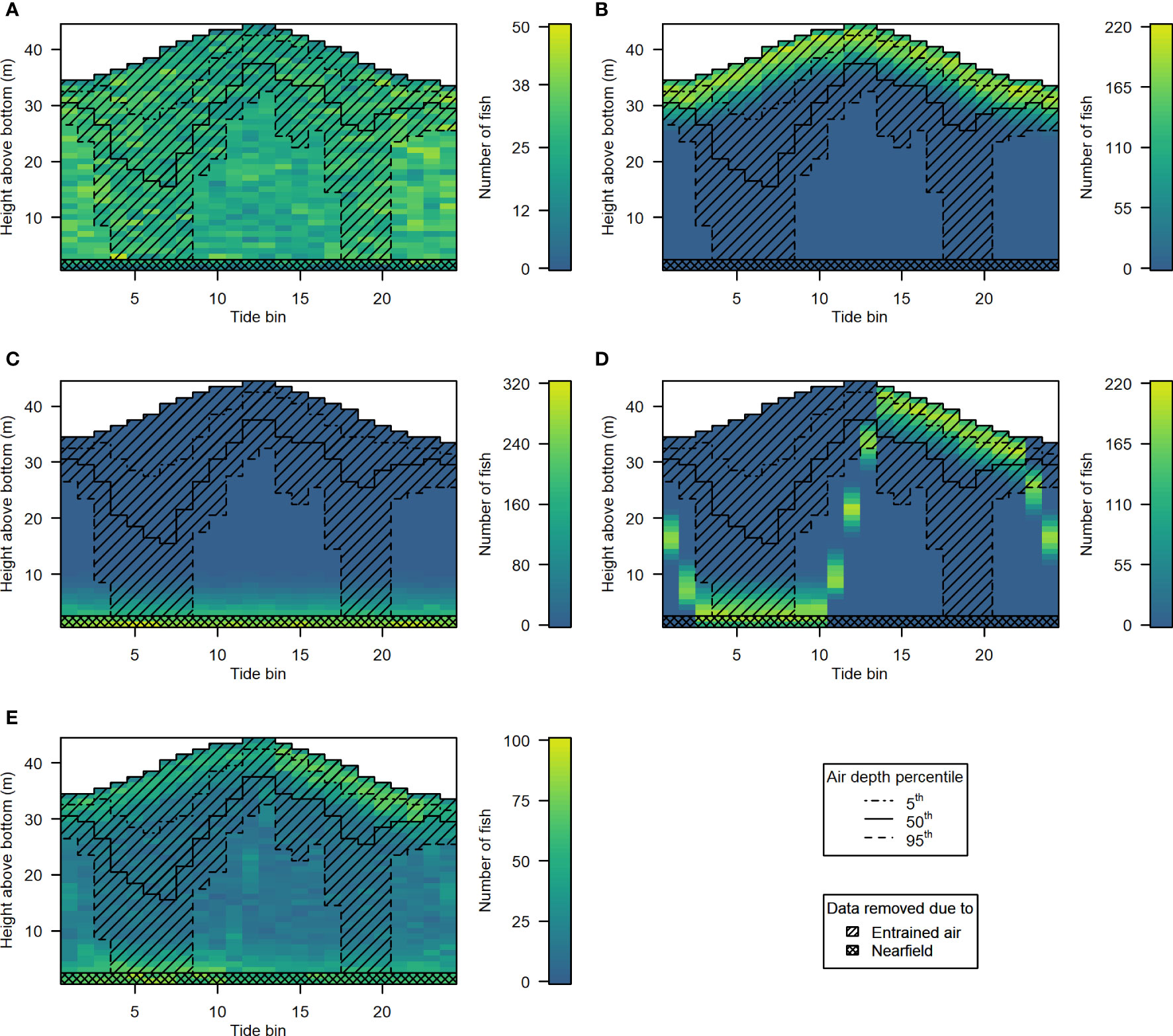
Figure 10 Hypothetical fish distributions generated for scenarios 1 to 5 [(A-E), respectively]. Color indicates the number of fish in each depth bin. Datapoints excluded by the 5^th (dot-dash line), 50^th (solid line), and 95^th (dashed line) percentile depth of the entrained air layer are indicated by the hatched area. The crosshatched rectangle covering the lowermost 2 m of the water column indicates the data that would be omitted due to the height of the acoustic nearfield above the sea floor.

FIGURE 11

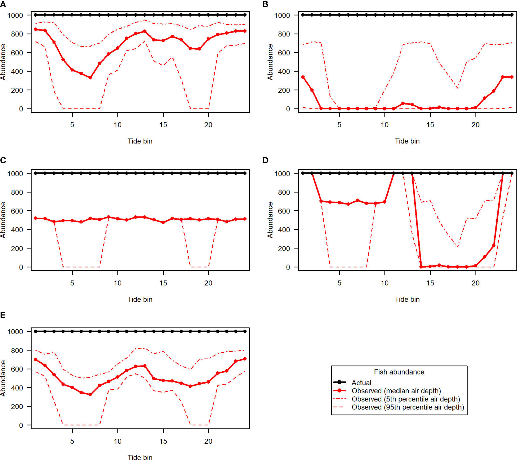
Figure 11 Fish abundance over the course of the tidal cycle for simulated fish distribution scenarios 1 to 5 [(A–E), respectively]. Actual abundance (black) is shown in contrast to abundance that would be observed under different levels of entrained air contamination (red lines).

The observed vertical distribution of fish was also heavily affected by the differing levels of entrained air contamination, as demonstrated with scenario 5 (Figure 12). Estimates of fish abundance in the uppermost portion of the water column were most affected, particularly during the running tides (ebb and flood) when entrained air extended the farthest. Even the best case situation, using the 5^th percentile of entrained air depths, resulted in excluding the majority of fish in the upper 10% (3.2-4.5 m depth) of the water column in all tidal stages, and the upper 20% (6.3-8.9 m depth) during flood tide. Due to the height of the acoustic nearfield above the sea floor, fish in the lowermost layers of the water column were also noticeably under-sampled.

FIGURE 12

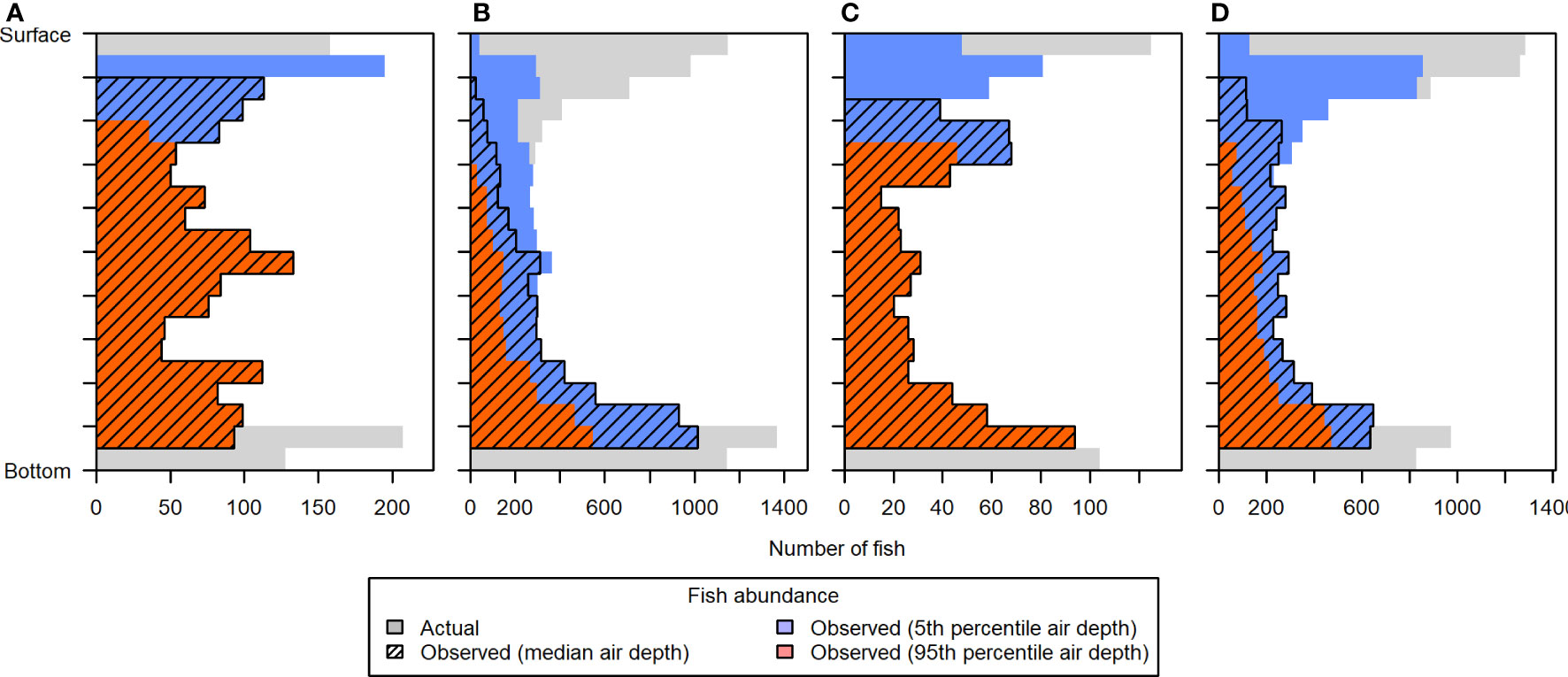
Figure 12 Vertical distribution of fish in simulated distribution Scenario 5, during (A) low, (B) flood, (C) high, and (D) ebb tide. The “actual” vertical distribution (light gray) is overlaid by the vertical distributions that would be observed under different levels of contamination by entrained air: 5^th percentile air depth (blue), 50^th percentile air depth (hatched), and 95^th percentile air depth (dark orange). Each depth bin spans 5% of the total water column depth, to facilitate comparison across tidal changes in water level. Fish counts in the lowermost two depth bins were primarily reduced due to the height of the acoustic nearfield above the sea floor.

4 Discussion

Active acoustics technologies provide more detail and breadth of information on fish throughout the water column than any other sampling method currently available. However, entrained air poses a significant problem for active acoustics data collected at tidal energy sites, and this must be considered when developing a study or environmental monitoring plan. The magnitude of entrained air contamination varies by site, and will be heavily dependent on local conditions (e.g. hydrodynamics, bathymetry, and weather; Baschek et al., 2006; Jech et al., 2021). The FORCE tidal energy test site has some of the fastest tidal currents on the planet (> 5 m·s^-1, Karsten et al., 2013), and its complex bathymetry and resulting dynamic current regime makes it one of the more challenging locations to use active acoustics instruments. Though the FORCE site is heavily affected by entrained air, the considerations discussed below will likely apply to echosounder users at other tidal energy test sites, as well.

Backscatter from entrained air contaminated 30% of all samples in our active acoustic dataset, and most of these were in the upper water column. However, contamination by entrained air varied greatly over time. The entrained air layer regularly spanned the entire water column during spring tides, though it rarely surpassed the middle water column during neap tides. So, while there were multiple days in a row with high levels of entrained air contamination, there were also periods of time with “best case” contamination levels, which would yield lower error rates in acoustically derived estimates of fish abundance. Peak current speeds were lower during neap tides than spring tides, but were well represented in the data throughout much of the water column. Active acoustics data collected near neap tides are therefore likely to consistently yield more complete information on fish abundance and vertical distribution than data collected closer to spring tides.

That being said, we found that the distribution of entrained air backscatter over the shorter time scales (e.g. during a tidal cycle) could magnify the error introduced to estimates of fish abundance and vertical distribution. In our simulations, the tidally fluctuating extent of the entrained air layer generated false tidal patterns in observed fish abundance, depending on the underlying vertical distribution of fish. The largest errors occurred when fish were mainly present in the uppermost layers of the water column, as this generated the strongest tidal pattern in estimated abundance (Figures 11B, D). Fish in the mid-water-column were increasingly omitted as current speed increased (Figures 11A, E). Abundance estimates of fish in the lowermost layers were mainly affected by the omission of data due to the height of the instrument above the sea floor and the extent of the acoustic nearfield, which introduced a constant negative bias (Figure 11C). Given the many species- and life-stage-specific depth preferences of fish, the prevalence of entrained air will therefore influence the extent to which different species are likely to be sampled by active acoustic instruments (for now ignoring other species-specific factors that affect detectability, such as their acoustic scattering properties; Horne, 2000).

The spatiotemporal fish distributions that we simulated were generalized examples of some commonly exhibited depth preferences among fish, and these may apply to many of the species likely to be in Minas Passage. For example, Scenario 1 may represent pelagic fish species that use most of the water column over the course of a day, including Atlantic herring, Atlantic mackerel, and striped bass (Castonguay and Gilbert 1995, Redden et al., 2014; Keyser et al., 2016; Viehman et al., 2018). Atlantic salmon, typically found in the uppermost 10 m in the northwest Atlantic, may be well-represented by Scenario 2 (Dutil and Coutu, 1988; Sheehan et al., 2012). The Minas Basin is inhabited by a large number of demersal species, such as Atlantic cod, Atlantic sturgeon (Acipenser oxyrhynchus), winter flounder (Pseudopleuronectes americanus), white hake (Urophycis tenuis), and dogfish (Squalus acanthius), among many others (Parker et al., 2007). Such species are likely to be on the seafloor or in the lowermost meters of the water column (e.g. Hobson et al., 2007), and therefore represented best by Scenario 3. Silver- and yellow- phase American eels have exhibited STST (Scenario 4) when migrating or moving around their home range, though with more frequent vertical movements during a tide and not always traversing the whole water column (Parker and McCleave, 1997). Other species have also exhibited STST, such as Atlantic cod (though with smaller vertical movements above the seafloor; Arnold et al., 1994; Hobson et al., 2009), and possibly Atlantic mackerel (Castonguay and Gilbert 1995). The cyclic changes represented by Scenario 4 could also be extended to diel differences in vertical distribution, which would bring fish into and out of the under-sampled layers of the water column on a 24-hour cycle (rather than 12-hour). Many species and life stages of fish exhibit some level of diel vertical migration; e.g. Atlantic herring (Huse et al., 2012; Viehman et al., 2018) and alosids (American shad, Alosa sapidissima; Alewife, A. pseduoharengus; and river/Blueback herring, A. aestivalis; Stone and Jessop, 1992). Scenario 5 may represent a mixed species assemblage, which is more realistic for this location; however, the proportions of fish exhibiting each type of distribution were chosen somewhat arbitrarily, as there is little information to base these on.

It is unknown whether species-specific depth preferences will persist in high-speed tidal channels. Apart from STST, most knowledge of different species’ depth distributions and vertical movements comes from measurements obtained in less energetic environments. Some information exists for tidal channels. Atlantic sturgeon, for example, are normally a demersal species, but acoustically-tagged sub-adults were found to transit Minas Passage pelagically (Stokesbury et al., 2016), slightly deeper during ebb tide than flood tide (Lilly et al., 2021). This could increase their detectability by active acoustics instruments (deployed as presented here), as individuals would be more likely to be in the middle-water-column rather than in the omitted layers near the sea floor. Eight acoustically tagged silver-stage American eels have been detected in the FORCE test site, and though they were mainly detected during ebb tide, they did not appear to exhibit the vertical motions associated with STST which this species has displayed elsewhere, instead utilizing most of the water column (Redden et al., 2014). Striped bass have been detected at the FORCE test site from summer through winter, carrying out diel vertical migrations from 20-40 m depth during the day to the upper 30 m at night, except at temperatures below 1˚C (Redden et al., 2014; Keyser et al., 2016). If Atlantic sturgeon, American eel, and striped bass all move pelagically at the FORCE site, then their availability to sampling by active acoustics may be best represented here by Scenario 1 (e.g., greater error in estimated abundance at peak flow). A better understanding of how different species utilize the water column in high-flow areas is necessary to assess their likelihood of sampling by active acoustic instruments.

Tidal and diel shifts in fish depth appear to be common across tidal energy sites, and these shifts could additionally influence the effects of entrained air on acoustically derived estimates of fish abundance and distribution. In Minas Passage, active acoustic measurements of fish (expected to be mainly overwintering Atlantic herring) found them to be more evenly spread out in the water column at night than during the day (Viehman et al., 2018), which was also observed throughout the year for a mixed fish assemblage in Cobscook Bay, USA (Viehman et al., 2015). In a tidal channel in Tasmania, Australia, fish were more closely associated with the surface at higher current speeds (Scherelis et al., 2020). In the Holyhead Deep, UK, European sprat (Sprattus sprattus) carried out diel vertical migrations linked to the depth of light penetration (Whitton et al., 2020), and in Admiralty Inlet, USA, the vertical location of fish and zooplankton changed on a 24-hour cycle (Gonzalez et al., 2019). Periodic vertical movements such as these could bring fish into and out of the entrained air layer at regular intervals. The possible interaction of this periodic movement with tidal patterns in entrained air depth could mask or generate patterns in observed fish abundance over time (as seen for Scenarios 4 and 5; Figures 11D, E). These considerations also apply to fish shifting their depth usage in response to deployed MHK devices; for example, avoiding a device by moving higher or lower in the water column, and therefore potentially into or out of the entrained air layer. There has been some evidence that marine animals (including fish and marine mammals) may change their swimming behavior in response to device presence (Williamson et al., 2021).

While the upper water column and higher current speeds (> 3 m·s^-1) were under-sampled in this dataset, the lower 70% of the water column was generally well-sampled for current speeds up to 3 m·s^-1 (Figure 7A). This is a large amount of data that can yield information on fish use of particular depth bins and how their depth may be influenced by a range of current speeds, all of which can inform our understanding of their likelihood of encountering an operating MHK device. However, information gained from a subset of the full range of depths and current speeds experienced at a site should not be assumed representative of the remaining, under-sampled depths and speeds. This is due to the above links between species, current speed, and depth usage, but also to other potential effects of current speed on fish behavior. For example, at a tidal energy site in the Pentland Firth, UK, fish school abundance and physical size was found to change as current speed surpassed 1 m·s^-1, potentially indicating an effect of physical forcing from tidal currents on schooling behavior (Fraser et al., 2018; Williamson et al., 2019). In these environments dominated by extreme physical forcing by tidal currents, it remains important to determine the extent to which information gathered at greater depths and lower speeds can be extrapolated (if at all). This could be examined at tidal energy sites that may have lower levels of entrained air contamination, or in future data collected with additional, complimentary sensors.

Additional sensing technologies will be essential for filling the gaps in active acoustics datasets that are left by entrained air, and for providing the necessary context for interpreting results. Acoustic telemetry has already provided valuable insight into when different species are likely to be present and where they are likely to be in the water column, and therefore how likely they are to be sampled with active acoustics in a deployment such as ours. Acoustically tagged individuals can be tracked over large distances, providing much-needed spatial context for the narrow volume sampled by an echosounder. Acoustic telemetry can help answer essential questions for building probability of encounter models, such as the proportion of a given fish population likely to come into the vicinity of a tidal turbine, and whether fish are actively swimming or drifting passively with the current. This adds to the information active acoustics provides for such models, which is fine-scale information on fish presence in the depths spanned by a given device, and how this changes over short and long time scales (for many more fish than can be tagged).

As with active acoustics, the efficiency of some acoustic telemetry systems can be reduced by current speed (Redden et al., 2014; Keyser et al., 2016; Tsitrin, 2019), resulting in fewer observations of fish location and depth during the time periods of greatest interest. This drop in detection probability could be related to the number of pulses that must be received from a given tag to allow a detection (Redden et al., 2014), the chance of a fish moving quickly past a receiver between acoustic tag transmissions (Keyser et al., 2016), as well as severe tilting of tethered receiver moorings in faster currents (Sanderson et al., 2017). These issues could be mitigated with appropriate choice of acoustic tags, mooring design, and receiver deployment (Sanderson et al., 2017; Sanderson et al., 2021). Recent experiments have shown drifting receivers could improve long-term tracking of individuals transiting Minas Passage, which wouldn’t necessarily be possible with fixed receiver arrays (Sanderson et al., 2021). A combination of active acoustics and acoustic telemetry, using both stationary and drifting receivers, could yield a much more complete picture of fish use of a tidal energy site and their chance of encountering MHK devices.

Fish activity within the entrained air layer itself may be quantifiable using optical techniques. While bubble plumes are largely “opaque” to active acoustic instruments, cameras may be less affected unless bubble density is very high. Video has been used for studying fish interactions with tidal energy turbines (Hammar et al., 2013; Broadhurst et al., 2014; Matzner et al., 2017), and in many other underwater applications requiring fish detection (e.g. Davidsen et al., 2005; Ellis and Bell, 2008). Optical systems cannot be used at night without additional lighting, which can affect fish behavior (Marchesan et al., 2005), and turbid or debris-laden water reduces fish detectability substantially (Ellis and Bell, 2008; Matzner et al., 2017). However, during daylight and with a few meters of visibility, there is an opportunity for video to be utilized for fish detection within the entrained air layer (Pattison et al., 2020). If optical data could be collected concurrently with an active acoustic system, ensuring sampled volumes overlap (or nearly do), results could help us understand how fish presence in the entrained air layer compares to abundance lower in the water column, and to what extent acoustically derived information from greater depths might be extrapolated upward.

Additional sensing technologies can help address another gap in active acoustics data analysis, which is the species and sizes of detected fish. This information would be helpful to those assessing the risk posed by tidal energy turbines, particularly when threatened or endangered species may be present. Information on fish species and length is also required to convert acoustic backscatter values to quantities of fish (Horne, 2000), unless fish are spread out enough to be detected and counted individually (e.g. Shen et al., 2016). Active acoustics data cannot usually provide identification of the detected scatterers to the species level without additional supporting information, which is typically obtained with trawls (Horne, 2000). The highly energetic and dynamic conditions at tidal energy sites often make them very difficult to sample safely or efficiently with trawls (Vieser et al., 2018), particularly at the spatial and temporal resolution required for classifying backscatter from a mixed assemblage within a rapidly changing environment. To date, most active acoustic studies at tidal energy sites have lacked physical sampling and stopped short of converting fish backscatter to estimates of abundance or biomass (Viehman et al., 2015; Fraser et al., 2018; Viehman et al., 2018; Staines et al., 2019; Williamson et al., 2019; Scherelis et al., 2020), with only one able to carry out concurrent trawling of a distinct layer of schools (Whitton et al., 2020).

Stereo optical camera or video systems may be useful alternatives to physically sampling fish at tidal energy sites. In recent years, species and length estimates from stereo camera systems have been found suitable for converting active acoustics backscatter to biological quantities, including in “untrawlable environments” (Rasmuson et al., 2021). Stereo optical systems are additionally non-lethal to sampled fish, less cumbersome than midwater trawls, and offer greater spatial resolution than trawls can provide (Boldt et al., 2018). Integrated optical-acoustic systems have been explored for MRE site monitoring, though so far only alongside high-frequency multibeam echosounders (Cotter and Polagye, 2020). Some challenges will need to be overcome for optical sensors to inform analysis of active acoustic data collected throughout the water column. As previously mentioned, optical systems require adequate lighting and water clarity for fish detection and identification. They also sample a much smaller volume than active acoustic instruments, which can complicate comparison to the larger volume sampled acoustically and can result in low sample sizes (Boldt et al., 2018). In addition to optical systems, acoustic tag detections could provide insight on the species in the area of an echosounder; however, only the species that were tagged would be detected, and any effects of high flow on detection probability would need to be addressed.

Using multiple acoustic frequencies could also broaden the information that can be gained from an active acoustic dataset. Data from multiple frequencies could aid in identifying different groups of scatterers (e.g. air bubbles, fish with and without swim bladders, zooplankton, etc.) based upon their frequency response (Horne, 2000; Korneliussen, 2018). The frequency response alone may not always be sufficient to identify fish to the species level without supporting information on which species are likely to be present. However, it is possible that the frequency response could be used to improve identification and removal of backscatter from entrained air bubbles. The entrained air detection method we used here relied mainly on morphological characteristics of the backscatter, which, for entrained air, mainly took the form of plumes extending downward from the surface. This is similar to methods used at other tidal energy locations (Viehman et al., 2015; Fraser et al., 2018; Whitton et al., 2020). Manual scrutiny of the data showed that backscatter from entrained air did not always take this form (e.g., when the entire water column appeared to be contaminated by additional backscatter; Figure 7), and there were many near-surface backscatter features that were not easily classified as fish or bubbles based on morphological criteria alone (Figure 5). Adding a frequency response filter to the morphological one applied here could improve backscatter classification, and further ensure that remaining backscatter is likely to be from fish.

Multiple acoustic frequencies could also aid in characterizing the entrained bubbles themselves, which would be useful for assessing whether they are likely to affect the performance of surface-mounted echosounders transmitting sound through the air layer to quantify fish below (Dalen and Løvik, 1981; Vagle and Farmer, 1991; Jech et al., 2021). To our knowledge, frequency response has not yet been used for identifying or characterizing entrained bubbles at tidal energy sites. However, this approach would be worth exploring in new or existing multifrequency datasets, as it can inform data collection moving forward.

5 Conclusion

Active acoustic technologies are well-suited for collecting information on fish abundance and distribution throughout the water column, with the resolution and breadth required for predicting the likelihood of fish occurring at the same depths as MHK devices. This information can add to our understanding of potential encounter rates, and therefore risk devices pose to fish. However, the prevalence of entrained air at tidal energy sites often masks large portions of the upper water column from echosounders, particularly at high current speeds. In the dataset examined, the lower 70% of the water column was well-represented for current speeds under 3 m·s^-1, but the upper water column and faster current speeds were under-sampled in comparison. These under-sampled depths and periods of time constitute gaps in the active acoustic dataset that limit our ability to accurately measure fish abundance and vertical distribution, and therefore their potential overlap with MHK devices. Additional technologies, such as acoustic telemetry and optical systems, could be used concurrently with active acoustics to help fill these gaps and maximize the information that can be extracted from active acoustics data. While other tidal energy sites may experience less data contamination from entrained air, patterns in data loss are likely to be similar. The possible influence of these patterns on acoustically derived measurements of fish abundance and vertical distribution must be considered when planning a study or environmental monitoring plan at a tidal energy site, and when interpreting results from active acoustic datasets.

Data Availability Statement

The raw data supporting the conclusions of this article will be made available by the authors, without undue reservation.

Author Contributions

HV, TB, and JD carried out preparation and planning of equipment deployment, including testing equipment settings and calibrating instruments. TB and JD deployed and retrieved the instruments. HV and JD processed the data. HV and DH contributed to the design of this study. HV completed the analysis, wrote the manuscript, and produced the tables and figures. All authors contributed to manuscript revision. All authors contributed to the article and approved the submitted version.

Funding

Data collection was funded by the Offshore Energy Research Association (project number 300-208).

Conflict of Interest

Author HV was employed by Echoview Software Pty Ltd.

The remaining authors declare that the research was conducted in the absence of any commercial or financial relationships that could be construed as a potential conflict of interest.

Publisher’s Note

All claims expressed in this article are solely those of the authors and do not necessarily represent those of their affiliated organizations, or those of the publisher, the editors and the reviewers. Any product that may be evaluated in this article, or claim that may be made by its manufacturer, is not guaranteed or endorsed by the publisher.

Acknowledgments

We would like to thank Huntley’s Diving and Marine Services (Mike Huntley and the crew of the Nova Endeavor) for making the safe deployment and retrieval of the FAST-3 platform possible. We also thank the members of the FORCE team, Dr. Louise P. McGarry, Dr. Joel Culina, and Lilli Enders, for assistance with understanding and interpreting the data.

Supplementary Material

The Supplementary Material for this article can be found online at: https://www.frontiersin.org/articles/10.3389/fmars.2022.851400/full#supplementary-material

References

Arnold G. P., Greer Walker M., Emerson L. S., Holford B. H. (1994). Movements of Cod (Gadus Morhua L.) in Relation to the Tidal Streams in the Southern North Sea. ICES J. Mar. Sci. 51, 207–232. doi: 10.1006/jmsc.1994.1021

CrossRef Full Text | Google Scholar

Baschek B., Farmer D. M., Garrett C. (2006). Tidal Fronts and Their Role in Air-Sea Gas Exchange. J. Mar. Res. 64, 483–515. doi: 10.1357/002224006778715766

CrossRef Full Text | Google Scholar

Boldt J. L., Williams K., Rooper C. N., Towler R. H., Gauthier S. (2018). Development of Stereo Camera Methodologies to Improve Pelagic Fish Biomass Estimates and Inform Ecosystem Management in Marine Waters. Fish. Res. 198, 66–77. doi: 10.1016/j.fishres.2017.10.013

CrossRef Full Text | Google Scholar

Broadhurst M., Barr S., Orme D. (2014). In-Situ Ecological Interactions With a Deployed Tidal Energy Device, an Observational Pilot Study. Ocean Coast. Manage. 99, 31–38. doi: 10.1016/j.ocecoaman.2014.06.008

CrossRef Full Text | Google Scholar

Castonguay M., Gilbert D. (1995). Effects of Tidal Streams on Migrating Atlantic Mackerel, Scomber Scombrus L. ICES J. Mar. Sci. 52, 941–954. doi: 10.1006/jmsc.1995.0090

CrossRef Full Text | Google Scholar

Copping A. E., Hemery L. G., Viehman H., Seitz A. C., Staines G. J., Hasselman D. J. (2021). Are Fish in Danger? A Review of Environmental Effects of Marine Renewable Energy on Fishes. Biol. Cons 262, 1–13. doi: 10.1016/j.biocon.2021.109297

CrossRef Full Text | Google Scholar

Cotter E., Polagye B. (2020). Automatic Classification of Biological Targets in a Tidal Channel Using Multibeam Sonar. J. Atmos. Ocean. Technol. 37, 1437–1455. doi: 10.1175/JTECH-D-19-0222.1

CrossRef Full Text | Google Scholar

Dalen J., Løvik A. (1981). The Influence of Wind-Induced Bubbles on Echo Integration Surveys. J. Acoust. Soc. Am. 69, 1653–1659. doi: 10.1121/1.385943

CrossRef Full Text | Google Scholar

Davidsen J., Svenning M.-A., Orell P., Yoccoz N., Dempson J. B., Niemelä E., et al. (2005). Spatial and Temporal Migration of Wild Atlantic Salmon Smolts Determined From a Video Camera Array in the Sub-Arctic River Tana. Fish. Res. 74, 210–222. doi: 10.1016/j.fishres.2005.02.005

CrossRef Full Text | Google Scholar

Demer D. A., Berger L., Bernasconi M., Bethke E., Boswell K., Chu D., et al. (2015). Calibration of Acoustic Instruments. ICES Cooperative Res. Rep. No, 326. doi: 10.17895/ices.pub.5494

CrossRef Full Text | Google Scholar

Dutil J. D., Coutu J. M. (1988). Early Marine Life of Atlantic Salmon, Salmo Salar, Postsmolts in the Northern Gulf of St. Lawrence. Fish. Bull. 86, 197–212.

Google Scholar

Ellis W. L., Bell S. S. (2008). Tidal Influence on a Fringing Mangrove Intertidal Fish Community as Observed by in Situ Video Recording: Implications for Studies of Tidally Migrating Nekton. Mar. Ecol. Prog. Ser. 370, 207–219. doi: 10.3354/meps07567

CrossRef Full Text | Google Scholar

Fraser S., Nikora V., Williamson B. J., Scott B. E. (2017). Automatic Active Acoustic Target Detection in Turbulent Aquatic Environments. Limnol. Oceanogr-Meth. 15, 184–199. doi: 10.1002/lom3.10155

CrossRef Full Text | Google Scholar

Fraser S., Williamson B., Nikora V., Scott B. (2018). Fish Distributions in a Tidal Channel Indicate the Behavioural Impact of a Marine Renewable Energy Installation. Energy Rep. 4, 65–69. doi: 10.1016/j.egyr.2018.01.008

CrossRef Full Text | Google Scholar

Gonzalez S., Horne J. K., Ward E. J. (2019). Temporal Variability in Pelagic Biomass Distributions at Wave and Tidal Sites and Implications for Standardization of Biological Monitoring. Int. J. Mar. Energy 2, 15–28. doi: 10.36688/imej.2.15-28

CrossRef Full Text | Google Scholar

Hammar L., Andersson S., Eggertsen L., Haglund J., Gullström M., Ehnberg J., et al. (2013). Hydrokinetic Turbine Effects on Fish Swimming Behaviour. PloS One 8, e84141. doi: 10.1371/journal.pone.0084141

PubMed Abstract | CrossRef Full Text | Google Scholar

Hobson V. J., Righton D., Metcalfe J. D., Hays G. C. (2007). Vertical Movements of North Sea Cod. Mar. Ecol. Prog. Ser. 347, 101–110. doi: 10.3354/meps07047

CrossRef Full Text | Google Scholar

Hobson V. J., Righton D., Metcalfe J. D., Hays G. C. (2009). Link Between Vertical and Horizontal Movement Patterns of Cod in the North Sea. Aquat. Biol. 5, 133–142. doi: 10.3354/ab00144

CrossRef Full Text | Google Scholar

Horne J. K. (2000). Acoustic Approaches to Remote Species Identification: A Review. Fish Oceanogr 9, 356–371. doi: 10.1046/j.1365-2419.2000.00143.x

CrossRef Full Text | Google Scholar

Huse G., Utne K. R., Fernö A. (2012). Vertical Distribution of Herring and Blue Whiting in the Norwegian Sea. Mar. Biol. Res. 8, 488–501. doi: 10.1080/17451000.2011.639779. 5-6.

CrossRef Full Text | Google Scholar

Jech J. M., Schaber M., Cox M., Escobar-Flores P., Gastauer S., Haris K., et al. (2021). Collecting Quality Echosounder Data in Inclement Weather. ICES Cooperative Res. Rep., 352. doi: 10.17895/ices.pub.7539

CrossRef Full Text | Google Scholar

Karsten R., Swan A., Culina J. (2013). Assessment of Arrays of in-Stream Tidal Turbines in the Bay of Fundy. Phil. Trans. R. Soc A. 371, 1985. doi: 10.1098/rsta.2012.0189

CrossRef Full Text | Google Scholar

Keyser F. M., Broome J. E., Bradford R. G., Sanderson B., Redden A. M. (2016). Winter Presence and Temperature-Related Diel Vertical Migration of Striped Bass (Morone Saxatilis) in an Extreme High-Flow Passage in the Inner Bay of Fundy. Can. J. Fish. Aquat. Sci. 73, 1777–1786. doi: 10.1139/cjfas-2016-0002. 12.

CrossRef Full Text | Google Scholar

Korneliussen R. J. (2018). Acoustic Target Classification. ICES Cooperative Res. Rep. No, 344. doi: 10.17895/ices.pub.4567

CrossRef Full Text | Google Scholar

Lilly J., Dadswell M. J., McLean M. F., Avery T. S., Comolli P. D., Stokesbury M. J. W. (2021). Atlantic Sturgeon Presence in a Designated Marine Hydrokinetic Test Site Prior to Turbine Deployment: A Baseline Study. J. Appl. Ichthyol. 37, 826–834. doi: 10.1111/jai.14274. 6.

CrossRef Full Text | Google Scholar

Marchesan M., Spoto M., Verginella L., Ferrero E. A. (2005). Behavioural Effects of Artificial Light on Fish Species of Commercial Interest. Fish. Res. 73, 171–185. doi: 10.1016/j.fishres.2004.12.009. 1-2.

CrossRef Full Text | Google Scholar

Matzner S., Trostle C., Staines G., Hull R., Avila A., Harker-Klimeš G. (2017). Triton: Igiugig Fish Video Analysis (PNNL-26576). Report to the U.S. Department of Energy (Richland, Washington: Pacific Northwest National Laboratory).

Google Scholar

Ona E., Mitson R. B. (1996). Acoustic Sampling and Signal Processing Near the Seabed: The Deadzone Revisited. ICES J. Mar. Sci. 53, 677–690. doi: 10.1006/jmsc.1996.0087

CrossRef Full Text | Google Scholar

Parker S. J., McCleave J. D. (1997). Selective Tidal Stream Transport by American Eels During Homing Movements and Estuarine Migration. J. Mar. Biol. Ass. U.K. 77, 871–889. doi: 10.1017/S0025315400036237

CrossRef Full Text | Google Scholar

Parker M., Westhead M., Service A. (2007). Ecosystem Overview Report for the Minas Basin, Nova Scotia (Fisheries and Oceans Canada, Dartmouth, NS: Oceans and Habitat Report 2007-05).

Google Scholar

Pattison L., Serrick A., Brown C. (2020). Testing 360 Degree Imaging Technologies for Improved Animal Detection Around Tidal Energy Installations. Final Report to the Offshore Energy Research Association of Nova Scotia (OERA) (Dartmouth, NS: Applied Oceans Research Group, Nova Scotia Community College).

Google Scholar

Rasmuson L. K., Fields S. A., Blume M. T. O., Lawrence K. A., Rankin P. S. (2021). Combined Video-Hydroacoustic Survey of Nearshore Semi-Pelagic Rockfish in Untrawlable Habitats. ICES J. Mar. Sci. 0, 1–17. doi: 10.1093/icesjms/fsab245

CrossRef Full Text | Google Scholar

R Core Team. (2021). R: A Language and Environment for Statistical Computing (Vienna, Austria: R Foundation for Statistical Computing). Available at: https://www.R-project.org/.

Google Scholar

Redden A. M., Stokesbury M. J. W., Broome J. E., Keyser F. M., Gibson A. J. F., Halfyard E. A., et al. (2014). Acoustic Tracking of Fish Movements in the Minas Passage and FORCE Demonstration Area: Pre-Turbine Baseline Studies (2011-2013). Final Report to the Offshore Energy Research Association of Nova Scotia and Fundy Ocean Research Centre for Energy (Acadia University, Wolfville, NS: Acadia Centre for Estuarine Research Technical Report No. 118).

Google Scholar

Sanderson B., Buhariwalla C., Adams M., Broome J., Stokesbury M., Redden A. (2017). Quantifying Detection Range of Acoustic Tags for Probability of Fish Encountering MHK Devices, In: EWTEC 2017: Proceedings of the 12th European Wave and Tidal Energy Conference; 2017 Aug 27 – Sep 1 (Cork, Ireland).

Google Scholar

Sanderson B., Stokesbury M. J. W., Redden A. M. (2021). Using Trajectories Through a Tidal Energy Development Site in the Bay of Fundy to Study Interaction of Renewable Energy With Local Fish. J. Ocean Technol. 16, 51–70. 1.

Google Scholar

Scherelis C., Penesis I., Hemer M. A., Cossu R., Write J. T., Guihen D. (2020). Investigating Biophysical Linkages at Tidal Energy Candidate Sites: A Case Study for Combining Environmental Assessment and Resource Characterization. Renew. Energy. 159, 399–413. doi: 10.1016/j.renene.2020.05.109

CrossRef Full Text | Google Scholar

Sheehan T. F., Reddin D. G., Chaput G., Renkawitz M. D. (2012). SALSEA North America: A Pelagic Ecosystem Survey Targeting Atlantic Salmon in the Northwest Atlantic. ICES J. Mar. Sci. 69, 1580–1588. doi: 10.1093/icesjms/fss052. 9.

CrossRef Full Text | Google Scholar

Shen H., Zydlewski G. B., Viehman H. A., Staines G. (2016). Estimating the Probability of Fish Encountering a Marine Hydrokinetic Device. Renew. Energy. 97, 746–756. doi: 10.1016/j.renene.2016.06.026

CrossRef Full Text | Google Scholar

Simmonds J., MacLennan D. N. (2005). Fisheries Acoustics: Theory and Practice (Oxford: Blackwell Science) 437 p.

Google Scholar

Staines G., Zydlewski G., Viehman H. (2019). Changes in Relative Fish Density Around a Deployed Tidal Turbine During on-Water Activities. Sustainability. 11, 2. doi: 10.3390/su11226262

CrossRef Full Text | Google Scholar

Stokesbury M. J. W., Logan-Chesney L. M., McLean M. F., Buhariwalla C. F., Redden A. M., Beardsall J. W., et al. (2016). Atlantic Sturgeon Spatial and Temporal Distribution in Minas Passage, Nova Scotia, Canada, a Region of Future Tidal Energy Extraction. PloS One 117, e0158387. doi: 10.1371/journal.pone.0158387

CrossRef Full Text | Google Scholar

Stone H. H., Jessop B. M. (1992). Seasonal Distribution of River Herring Alosa Pseudoharengus and A. Aestivalis Off the Atlantic Coast of Nova Scotia. Fish. Bull. 90, 376–389.

Google Scholar

Tsitrin E. (2019). Sofishticated Tracking: Improved Protocol for Acoustic Tagging of Sensitive Clupeid Fishes, and Applications in Investigating Postspawning Migration of Alewife (Alosa pseudoharengus) in Minas Basin, Bay of Fundy. [Master’s thesis]. Wolfville (NS): Acadia University.

Google Scholar

Vagle S., Farmer D. M. (1991). The Measurement of Bubble-Size Distributions by Acoustical Backscatter. J. Atmos. Ocean. Technol. 9, 630–644. doi: 10.1175/1520-0426(1992)009<0630:TMOBSD>2.0.CO;2

CrossRef Full Text | Google Scholar

Viehman H., Boucher T., Redden A. (2018). Winter and Summer Differences in Probability of Fish Encounter (Spatial Overlap) With MHK Devices. Int. J. Mar. Energy 1, 9–18. doi: 10.36688/imej.1.9-18. 1.

CrossRef Full Text | Google Scholar

Viehman H., Zydlewski G., McCleave J., Staines G. (2015). Using Hydroacoustics to Understand Fish Presence and Vertical Distribution in a Tidally Dynamic Region Targeted for Energy Extraction. Estuaries Coast 38, 215–226. doi: 10.1007/s12237-014-9776-7. 1.

CrossRef Full Text | Google Scholar

Vieser J. D., Zydlewski G. B., McCleave J. D. (2018). Finfish Diversity and Distribution in a Boreal, Macrotidal Bay. Northeastern Nat. 25, 545–570. doi: 10.1656/045.025.0403. 4.

CrossRef Full Text | Google Scholar

Whitton T. A., Jackson S. E., Hiddink J. G., Scoulding B., Bowers D., Powell B., et al. (2020). Vertical Migrations of Fish Schools Determine Overlap With a Mobile Tidal Stream Marine Renewable Energy Device. J. Appl. Ecol. 57, 729–741. doi: 10.1111/1365-2664.13582

CrossRef Full Text | Google Scholar

Williamson B. J., Blondel P., Williamson L. D., Scott B. E. (2021). Application of a Multibeam Echosounder to Document Changes in Animal Movement and Behaviour Around a Tidal Turbine Structure. ICES J. Mar. Sci. 78, 1253–1266. doi: 10.1093/icesjms/fsab017

CrossRef Full Text | Google Scholar

Williamson B., Fraser S., Williamson L., Nikora V., Scott B. (2019). Predictable Changes in Fish School Characteristics Due to a Tidal Turbine Support Structure. Renew. Energy 141, 1092–1102. doi: 10.1016/j.renene.2019.04.065

CrossRef Full Text | Google Scholar

Woolf D. K. (2001). “Bubbles,” in Encyclopedia of Ocean Sciences (Cambridge, MA: Academic Press), 352–357. doi: 10.1006/rwos.2001.0062

CrossRef Full Text | Google Scholar