 Nina Dehnhard1*
 Jenny Mattisson1
 Arnaud Tarroux2
 Tycho Anker-Nilssen1
 Svein-Håkon Lorentsen1Signe Christensen-Dalsgaard1
- 1Department of Terrestrial Ecology, Norwegian Institute for Nature Research (NINA), Trondheim, Norway
- 2Department of Arctic Ecology, Norwegian Institute for Nature Research (NINA) – Framsenteret, Tromsø, Norway
Human activity in the coastal zone is increasing worldwide, putting a number of seabird species under pressure. Norway is no exception to this development, and with > 35% of the NE Atlantic population of the currently declining European shag (Gulosus aristotelis) population, Norway has an international responsibility for the conservation of this species, and its important foraging habitats during breeding. We analysed tracking data from shags breeding in five colonies along the Norwegian coast spread over a latitudinal gradient of > 1700 km. We identified foraging locations and associated environmental characteristics. Using model cross-validation, we assessed the transferability of habitat models, both spatially (across colonies) and temporally (within colonies and across years), based on three modelling approaches: Training datasets consisted either of the data from one year at one colony, all years at one colony, or all years from all colonies except the testing colony. Across colonies, foraging activity was associated with shallow depths, proximity to colony, and the presence of kelp forests, while sea surface temperature and sea surface height contributed little to model fit. Transferability of habitat use across colonies was low when based on the training data from only one year and one colony and improved little when using several years of data from one colony for training the models. Transferability was very high for all colonies if the training dataset consisted of data from all years and all colonies except the one to be predicted. Our results highlight the importance of multi-year and multi-colony studies and show that it is possible to make sound fine-scale predictions of important foraging areas for breeding shags without the need to track birds in every colony. This facilitates much needed management of coastal marine ecosystems and the protection of the most important feeding areas for breeding shags.
Introduction
Coastal zones, although widely acknowledged to be of high ecological and economic value, are also highly vulnerable and impacted by a multitude of human activities (Crain et al., 2008; Brown et al., 2018). These impacts have profound effects on entire food webs, from primary producers to top-predators (Worm et al., 2006; Worm et al., 2009; Poloczanska et al., 2013). Marine spatial planning, and the creation of Marine Protected Areas (MPAs) are increasingly used to counteract the potential detrimental effects of human activities on marine ecosystems (Edgar et al., 2014; Halpern et al., 2015).
Seabirds are among the most threatened taxonomic groups of birds, facing a multitude of mostly anthropogenic stressors (Dias et al., 2019). These range from oil exploration (Votier et al., 2005; Votier et al., 2008), establishment of wind farms (Garthe and Hüppop, 2004; Furness et al., 2013; Peschko et al., 2020), kelp harvesting (Lorentsen et al., 2010; Christensen-Dalsgaard et al., 2020), bycatch (Anderson et al., 2011; Žydelis et al., 2013), ship traffic (Dehnhard et al., 2020a) and fisheries (Cury et al., 2011; Saraux et al., 2020) to various impacts of climate change (e.g. Grémillet and Boulinier, 2009; Keogan et al., 2018), but also include predation by introduced predators (Craik, 1997). Although these stressors affect seabird species differently, and their impact varies geographically, many of them act to make seabird foraging areas particularly relevant for protection (e.g. Davies et al., 2021). Previous approaches to identify important foraging areas for breeding seabirds have largely been based on an existing toolkit by BirdLife International (2010). Where feasible, tracking data, ideally collected over several years, should be used to identify important foraging areas (e.g. Lascelles et al., 2016). Since it is highly unrealistic to track individuals of all species in all colonies, the next best alternative has been to use a standardised foraging range radius around each colony to define the areas most likely used by the seabirds (BirdLife International, 2010; Thaxter et al., 2012). The foraging radius approach is, however, likely to result in the inclusion of substantial areas that are not regularly used by birds for feeding (Thaxter et al., 2012; Soanes et al., 2016). A refinement of this approach, using for example additional environmental covariates such as depth has been suggested (Soanes et al., 2016). An alternative solution could be to predict important foraging areas for a given population based on tracking information from birds in other colonies. This approach has so far been attempted only for a few pelagic seabird species, with varied success (e.g. see Torres et al., 2015; Péron et al., 2018; Fauchald et al., 2021), but to the best of our knowledge not for coastal seabird species.
The European shag (Gulosus aristotelis, hereafter: shag) is a coastal benthic foraging seabird with an all-year coastal distribution. In Norway, which had approximately 28,000 breeding pairs in 2013 (Fauchald et al., 2015), constituting about 35% of the NE Atlantic population (Mitchell et al., 2004), shags breed in hundreds of colonies scattered all along the entire western and northern coastlines (Figure 1). While information about critical foraging habitats is highly relevant for management purposes, it remains an unrealistic task to track shags from every colony. The species therefore represents an ideal case to test whether important foraging areas can be accurately identified for one colony based on habitat use in another colony.
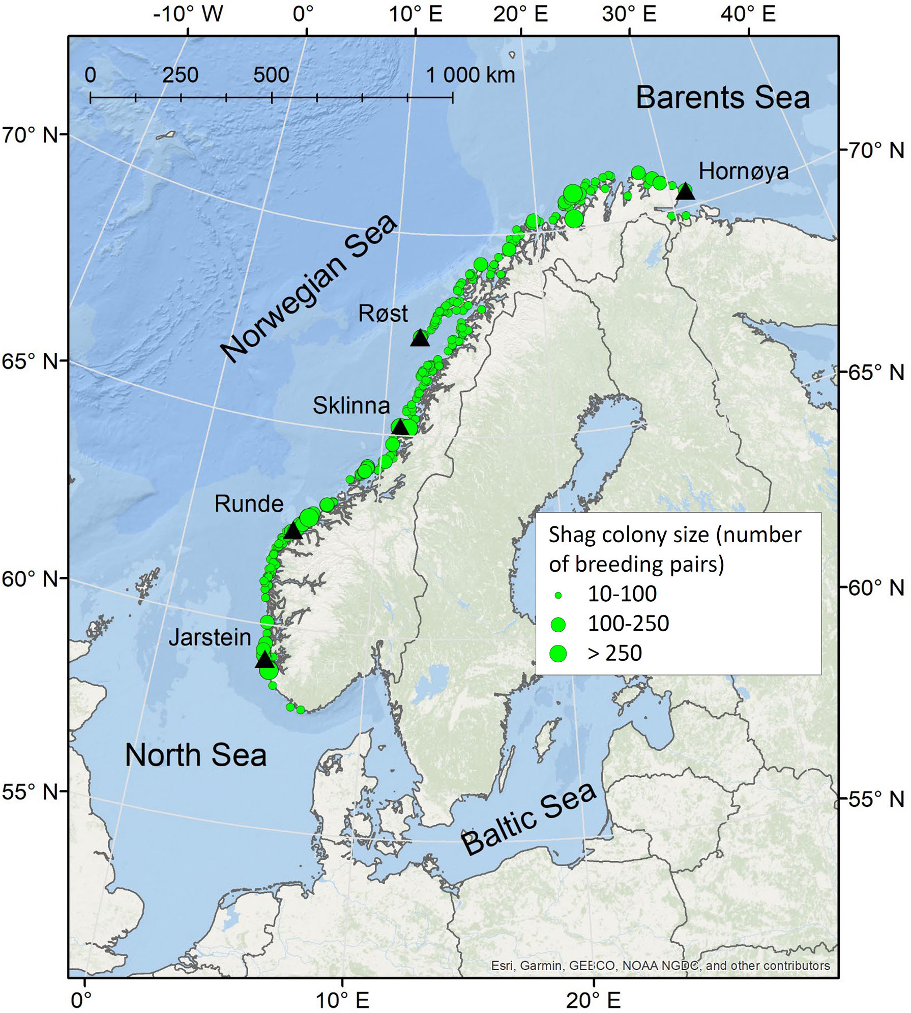
Figure 1 Overview map showing the locations of the five shag study colonies in Norway (black triangles). Green points indicate the location and approximate size of all shag colonies registered through the national seabird monitoring programme in Norway.
Shags primarily feed on fish (e.g. Hillersøy and Lorentsen, 2012; Howells et al., 2018) and typically show shallow diving patterns in the range of about 15-20 m, although they can dive down to 60 m (Wanless et al., 1997; Evans et al., 2016; Christensen-Dalsgaard et al., 2017). As other seabirds, the species exhibits a typical central-place foraging behaviour during the breeding period (Bell, 1990) with a maximum foraging range of about 20-40 km around their colonies (Bogdanova et al., 2014; Lorentsen et al., 2019). Shags are vulnerable to disturbance by boats (Velando and Munilla, 2011), and incidental mortality in gillnet fisheries (Žydelis et al., 2013; Christensen-Dalsgaard et al., 2019). Furthermore, kelp harvesting in areas used by shags for foraging has the potential to affect foraging success (Christensen-Dalsgaard et al., 2020). Finally, aquaculture installations can easily lead to a reduction in available coastal marine habitat, increased boat traffic and therefore higher disturbance effects, and shags are perceived as a pest by the aquaculture industry (Beveridge, 2001). Licences to cull (shoot) shags are issued on such grounds where shags are expected to cause damage (BirdLife International, 2016).
We tracked breeding shags with GPS loggers in five colonies spread along the Norwegian coast (Hornøya, Røst, Sklinna, Runde and Jarstein; Figure 1). The overarching goal of this study was to identify the foraging areas and associated environmental characteristics in all five colonies and assess the transferability of models of habitat use within colonies (across years; temporal transferability) and across colonies (spatial transferability). Model transferability is a central issue in conservation ecology (Yates et al., 2018; Matthiopoulos et al., 2022), and in the context of our study transferability both within and across colonies is key to sound protecting of foraging areas utilised by shags without having to track birds each year or from each colony.
We first (aim 1) investigated the habitat characteristics and variability in fine-scale (< 1 km) habitat use of shags breeding in the different colonies. Since variability in habitat use within colonies might have confounding effects on the transferability of results from one colony to another, we assessed if the data from one year could be used to predict the habitat use in another year within the same colony (i.e. ‘transferability within colonies’). Aim 2 was to assess the predictability of fine-scale habitat use in a given colony based on environmental habitat characteristics in one or several other colonies (‘transferability across colonies’). With this in mind, we set up three different modelling approaches with different training datasets, in order to find the approach that delivered the best results for transferability across colonies.
We hypothesised that distance to colony would be an important variable in the models describing foraging habitat use, but that foraging range would differ across colonies, e.g. due to inter-colony differences in the number of breeding pairs sharing the foraging grounds (e.g. Jovani et al., 2016). Based on previous studies (Christensen-Dalsgaard et al., 2017; Grémillet et al., 2020), we further expected that foraging habitats would be characterised by shallow depths and the presence of kelp forests or sandy bottom, representing the habitat preferences of their main prey; gadids (e.g. Hillersøy & Lorentsen, 2012) and sandeel (Ammodytes spp., Howells et al., 2018), respectively. Spatial variation in sea surface temperature (sst) and sea surface height (ssh) are typically associated with frontal zones and eddies in the pelagic environment (e.g. Kostianoy et al., 2004; Mason et al., 2014), and upwelling plumes over continental shelves (e.g. Ainley et al., 2009). These variables tend to be important to characterise the habitat of pelagically foraging seabirds (e.g. Pinaud and Weimerskirch, 2005), but we expected them to be less important variables to characterise foraging habitats of the coastal-feeding shags. Finally, we hypothesised that – similar to findings in other seabirds (Péron et al., 2018) – shags breeding in colonies located closer to each other would be more similar in their habitat use compared to colonies further away, and thus that across-colony transferability of the models would decrease with distance between colonies.
Methods and Material
Fieldwork was conducted at Hornøya (70°23’N, 31°09’E; 630 breeding pairs in 2012), Ellefsnyken/Røst (67°27’N, 11°55’E; 345 breeding pairs in 2020), Heimøya/Sklinna (65°12’N, 10°59’E; 2000 breeding pairs on average in 2011-2020), Runde (62°23’N, 5°36’W; 150 breeding pairs in 2020), and Jarstein (59°09’N, 5°10’E, 274 breeding pairs in 2020). These five colonies (Figure 1) together represent approximately 10-15% of the total Norwegian shag population and are focal study colonies for the species in the long-term monitoring and mapping programme for Norwegian seabirds, SEAPOP (www.seapop.no/en). Notably, at Hornøya, Røst and Jarstein there are additional, neighbouring shag colonies, located within the foraging ranges of the above-listed study colonies. We do not have exact population numbers for these other shag colonies, but the approximate total number of shag breeding pairs sharing the foraging area was 1000 at Hornøya, 1000 at Røst and 600 at Jarstein. A colony was here defined as an aggregation of more than 10 nests at a given location (e.g. on a single island).
Shags were equipped with either a GPS logger or a combination of a GPS and a temperature-depth (TDR) logger (Table S1.1, Supplement 1). The logger types used were I-gotU GT-120 GPS loggers (Mobile Action Technology, modified and re-fitted in heat shrink tubes, 24 g) and remote-downloading solar-driven PathTrack GPS loggers (PathTrack nanoFix® GEO+RF, 21.8 g), as well as G5 TDR-loggers (CEFAS Technology, 6.5 g). I-gotU loggers were programmed to record data at either 30 or 60 second intervals (Table S1.1, Supplement 1). PathTrack loggers were programmed to record data on a solar-power-based schedule at either ≥ 30 sec (only a short trial in 2020 at Sklinna) or ≥ 5 min intervals (majority of deployments), with a download frequency of 30 min or less via UHF to a fixed base-station positioned within 500 m of the nests. The GPS sampling rates of PathTrack loggers thus automatically downscaled when batteries got depleted (e.g. from 5 min to 10 min, and subsequently 15 min, 20 min, 25 min and so on). Averaged across colonies and years, PathTrack loggers obtained GPS fixes at intervals every 11.75 ± 30.1 min (average ± SD). TDR loggers recorded data at 1 or 2 second intervals. I-gotU and TDR loggers were joined with tape prior to the deployment and attached to 3-4 middle tail feathers using strips of Tesa tape. PathTrack loggers were also attached to the middle tail feathers, using a thin plastic-plate and a combination of tape and cable ties. Those birds that were equipped with both a PathTrack logger and a TDR, were fitted with a plastic leg-ring to which the TDR-logger was attached. GPS and TDR loggers combined weighed at maximum 31 g, corresponding to < 1.7% and < 1.9% of the mean body mass of males and females, respectively.
The nests used in this study were randomly selected among those nests that had approachable adults, and attempts were made to capture equal numbers of males and females when sampling the individuals. Adults were caught on the nest by hand or a noose pole, and sex was determined by size and vocalization (cf. Cramp and Simmons, 1977). The majority of shags deployed with GPS loggers were rearing chicks when loggers were deployed, but some were still in the late phase of incubation (Table S1.1, Supplement 1). Birds deployed with I-gotU loggers were recaptured after 1-3 days to recover the devices, and the same happened with the trial birds deployed with PathTrack loggers programmed at the ≥ 30 sec schedule in 2020 at Sklinna. Birds deployed with PathTrack loggers and TDR loggers (combined deployment only at Sklinna) with GPS fixes ≥ 5 min were recaptured after 14-18 days to retrieve the TDR-loggers, but the PathTrack loggers remained attached until they fell off when tail feathers were moulted. Birds deployed with only PathTrack loggers (without TDRs) were not recaptured, and loggers remained attached until the birds moulted their tail feathers. Deployments with I-gotU loggers usually did not take longer than 3 min, while those with PathTrack loggers usually took less than 10 min.
Subsequent GPS Data Analyses
We obtained data from a total of 550 GPS deployments (Table S1.1, Supplement 1). Following Lorentsen et al. (2019), we excluded locations within 500 m of their nest sites at all colonies, since these locations are mostly associated with resting and preening activities as well as washing dives. As such, this near-colony habitat is important for the shags but does not represent important foraging habitat. Similarly, any roosting places at or near foraging sites were removed, i.e. when GPS locations were located on land and not at sea. GPS data after the chicks were fledged was excluded from the analysis, assuming a fledging age of 57 days, based on Daunt et al. (2007). Apparent locational outliers were removed using a speed filter with a maximum speed of 30 m/s, and a speed filter of 15 m/s on strongly curvaceous flight paths, as described in Lorentsen et al. (2019).
Following Lorentsen et al. (2019), we defined foraging trips as movement paths ≥ 5 min ≥ 500 m away from the colony. For comparing foraging trip metrics across colonies, we excluded incomplete foraging trips: i.e. trips where 1) locations at the colony were not available either before or after the trip, 2) gaps of > 30 minutes (to account for the GPS-intervals of PathTrack loggers) existed between the last and or first location in the trip and the next or previous location at the colony, and 3) gaps of > 60 minutes existed between locations during the trip. Due to the inability of GPS loggers to acquire locations when submerged (i.e. when the bird is diving), trips recorded by both logger types frequently included gaps between GPS locations. The one-hour cut-off to define incomplete trips was chosen as a conservative measure based on average trip duration (see Table 1) and the obtained GPS-intervals.
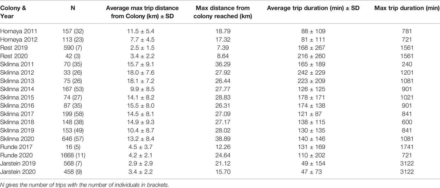
Table 1 Foraging trip metrics per colony and year obtained from complete foraging trips (see Methods).
We identified likely foraging locations of shags based on expectation-maximization binary clustering (EMbC) of the GPS locations (Garriga et al., 2016b). EMbC uses velocity and turning angle to classify movement data into four different clusters aligned with likely behavioural states: low velocities and low turns (LL; “resting”), low velocities and high turns (LH; “intensive search”), high velocities and low turns (HL; “travelling”) and high velocities and high turns (HH; “extensive search”) (Garriga et al., 2016b). EMbC has been shown to be useful across a broad range of species (e.g. Cecere et al., 2020; De Pascalis et al., 2020; Dehnhard et al., 2020b) and comes with the advantage of requiring less supervision, less a-priori assumptions and less computational power than other approaches (Garriga et al., 2016b).
GPS data were analysed in the R-package EMbC (Garriga et al., 2016a), using the stack clustering function (stbc), which accounts for potential among-individual behavioural differences by annotating behavioural states for each individual. The stack clustering function was run pooled for all data from all colonies and all years, in order to guarantee the same cut-offs across colonies and years. The pre- and post-smoothing options were set to zero.
To test the performance of our EMbC-based approach to identify foraging locations, we used known diving locations from the colonies and years where TDR data were available (Supplement 1). Summary statistics of dive depth and dive duration are presented in Table S1.2, Supplement 1. We found a high spatial overlap between the known dive locations and EMbC-states LL (“resting”) and LH (“intensive search”): More than 81% of known dive locations were spatially close (within 200 m) or identical to locations that the EMbC algorithm identified as LL and LH (see Table S1.3, Supplement 1). All GPS time-stamps with EMbC states LL and LH were thus defined as foraging locations in further analyses. By doing so, we might characterise some fixes as foraging locations that in fact were not foraging locations, but which still represent an area birds were commuting through.
Environmental Variables
To characterise the habitat use of the shags, we selected five environmental variables, all of which have previously been shown to be important determinants of foraging areas for this species (Christensen-Dalsgaard et al., 2017; Grémillet et al., 2020): bathymetry, slope, kelp presence, sst and ssh. We downloaded bathymetry data from GEBCO (https://www.gebco.net/data_and_products/gridded_bathymetry_data/; spatial grid of 450x450m). Sea bottom slope (in degrees) was calculated from the bathymetry data as the maximum change from the cell to its eight closest neighbours using the raster package in R (Hijmans, 2021). Kelp data were obtained from The Norwegian Environmental Agency (https://geocortex01.miljodirektoratet.no/Html5Viewer/?viewer=naturbase). Daily sst and ssh data were obtained from the Norkyst800m model (at a spatial resolution of 800x800m; Albretsen et al., 2011). These data were provided by the Norwegian Meteorological Institute on request for the entire study period, and were obtained from a model version that produced consistent results over this period of time (see Asplin et al., 2020). Instead of working with daily sst and ssh values, which would have substantially complicated our modelling approach, we calculated their means and temporal variances over the period 1st of June – 15th of July for each year. These dates correspond on average to a period of 2 weeks before the first GPS deployment and up to – for most sites and years – the retrieval of the last GPS loggers/data (see Table S1.1, Supplement 1), and were consistently used for all colonies. The two-week period prior to the (on average) first deployment was chosen since sst and ssh may affect prey availability and distribution over a longer period of time, and thus may have a lagged effect.
Sea bottom substrate data, which have been proven an important environmental covariate for shag foraging habitats (Grémillet et al., 2020), were downloaded from the European Marine Observation and Data Network (EMODnet) (http://gis.ices.dk/geonetwork/srv/eng/catalog.search#/metadata/01bf1f24-fdcd-4ee7-af8b-e62cf72fe2f9). Unfortunately, data quality in the coastal areas were poor and for 57% of the likely foraging locations, the substrate type was unknown. We therefore refrained from including sea bottom substrate into our analyses.
Definition of Available Habitat - Creation of Random Points
We followed the approach of Christensen-Dalsgaard et al. (2017) and defined available habitat as the area within reach for breeding birds around their colonies, and thus created a circular buffer around each colony. The radius of this buffer was set as the maximum distance between a foraging location and the colony, which was largest for Sklinna (40 km), followed by Runde (25 km), Jarstein (22 km), Hornøya (19 km) and Røst (9 km). To create a representative sample of available habitats within these areas, five point locations were created randomly for each GPS fix defined as a foraging location within the defined available area, using the R-package sp (Pebesma and Bivand, 2005; Bivand et al., 2013). As we include temporal environmental variables in the model, the process was done separately for each year. Land areas within the circular buffers were removed before generating random locations. All foraging locations and random locations were intersected with the environmental layers using the function “extract” in R-package raster.
Modelling Approach
All statistical procedures were carried out in R (R Development Team, 2020). To assess if maximum foraging distance differed across colonies, we ran a linear mixed-effects model (LMM) using function lmer from package lme4 (Bates et al., 2015). The LMM contained maximum trip distance from the colony (only for complete foraging trips) as dependent variable, and colony as explanatory variable (factor). Bird ID was included as a random factor, nested within year and colony. We further present marginal and conditional R2 values as calculated from the R-package performance (Lüdecke et al., 2021) and to identify differences among colonies, we ran a Tukey post-hoc test (R-package multcomp; Hothorn et al., 2008).
To investigate marine habitat preferences (aim 1), we ran generalised additive models (GAMs) with a binomial distribution (1 = foraging locations, 0 = availability, i.e. random locations). GAMs were run using the R-package mgcv (version 1.8-38; Wood, 2017) with a logit link function. Generalised additive models allow the fitting of non-linear responses to predictor variables, which is a major advantage, as animals rarely respond linearly to their environment (Aarts et al., 2008; Dehnhard et al., 2020b). Similarly to Christensen-Dalsgaard et al. (2017), GAMs were fitted using thin plate regression smoothing (Wood, 2017). We initially set the maximum number of knots for smooth terms to 5 in order to avoid overfitting, and used the functions “gam.check” to check whether models with more knots had a better fit. We followed a forward-stepwise approach to add environmental covariates, and modelled the environmental habitat preferences separately for each colony. The initial models therefore contained year (as a fixed factor), and one environmental covariate, either as fixed factor (kelp) or as smooth term (depth, slope, distance to colony, sst mean, sst variance, ssh mean, ssh variance). After identifying the best-performing smoothed environmental variable, we assessed the inclusion of kelp, and then subsequently of a second and third smoothed environmental variable. To avoid collinearity among environmental covariates, we only included those that had a Spearman’s rank correlation of ≤ 0.5. Model selection was based on AIC, and we did not attempt to fit more than three smooth terms into the final model to avoid over-fitting. We calculated Akaike weights (wi) for all models following Burnham & Anderson (2002).
After identifying the best model structure for each colony, we investigated the transferability of the results within colonies and across colonies. We used model cross-validation, and the dataset was divided into a training dataset to fit the model, and a testing dataset to assess its performance. We used the area under the receiver curve (AUC; pROC package; Robin et al., 2011) to assess performance of models. AUC values <0.7 were considered poor, 0.7 to 0.9 reasonable, and >0.9 very good model performance. To investigate transferability across years within the same colony, the testing dataset consisted of one year of data, and the training dataset of another year of data from the same colony, similarly as performed by Péron et al. (2018). For Sklinna, where we had ten years of data, we also assessed if transferability across years could be improved by training the dataset with nine years of data (instead of only one) and using the remaining year as test dataset (similar to Fauchald et al., 2021). When assessing the transferability across colonies (aim 2), we applied three different strategies to train models in order to see which one would deliver the best results, and whether increasing the variation within the training dataset could improve the between-colony transferability.
Firstly (“individual colony and year approach”), both the training and the testing dataset consisted of data from one colony and one year each, and AUC values were calculated for all combinations of colonies and years. This approach thus followed the same strategy as that by Péron et al. (2018). The best fitting model for the training dataset was chosen as model structure. With this approach, we thus attempted to predict the foraging habitat of the birds in one colony during one specific year based on the model structure based on the habitat use of birds in another colony during one year (same or different year).
Secondly (“individual colony approach”), the training and the testing dataset consisted of all data from all years of a given colony, and AUC values were calculated for all combinations of test colonies. The model structure was based on the best fitting model for the training dataset (i.e. as in the individual colony and year approach). With the individual colony approach, we thus attempted to predict the foraging habitat of the birds in one colony across several years based on the model structure, data and habitat use of birds in another colony during 2+ years.
Thirdly and lastly (“all colonies approach”), the training dataset consisted of all data from all colonies and years, with exception of the testing colony, and AUC values were calculated using each colony as a test colony once. Since the environmental predictors retained in the best model varied between colonies (Table 2), we had to use a simplified model structure, and only included kelp, depth and distance to colony in the models (i.e. those static variables that were consistently supported in the models for all colonies), but none of the temporally variable environmental variables (i.e. means or variances in sst and ssh). The motivation for the all colonies approach was to test if a larger and more diverse training dataset from four colonies with 2+ years of data each would be suitable to predict the habitat use in a fifth colony. This approach was based on the assumption that the temporally variable environmental covariates (see Supplement 2) would not contribute much to explain the habitat use across colonies compared to the temporally static ones (kelp, depth and distance to colony).
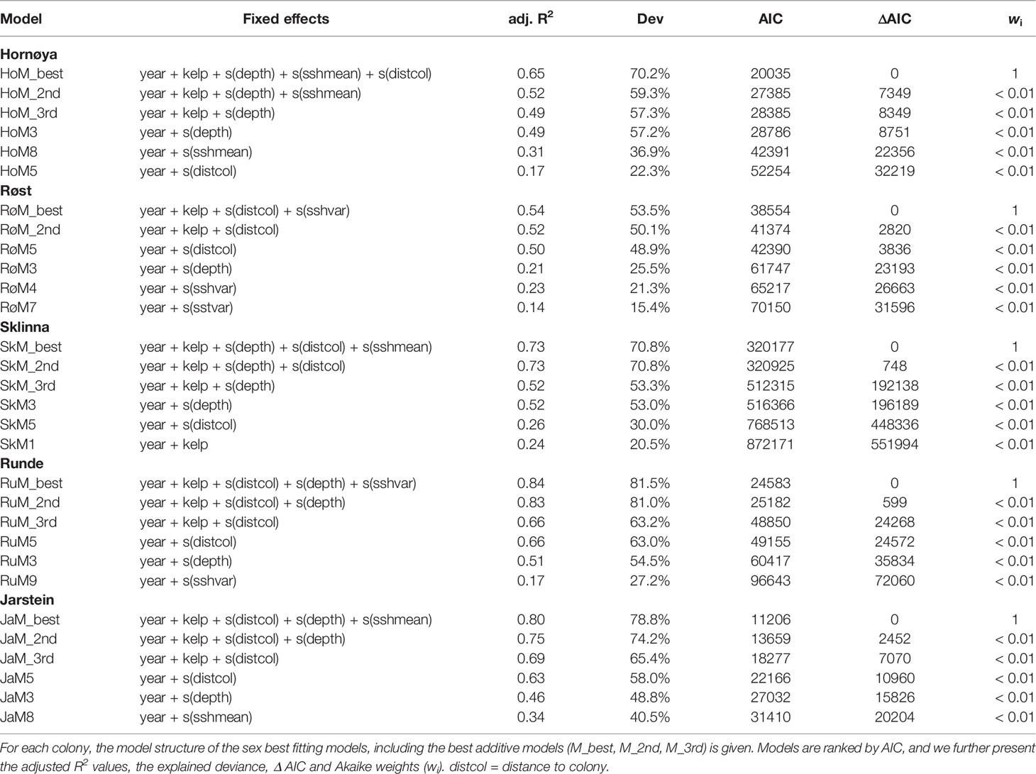
Table 2 Summary of the model selection process.
Results
We found strong evidence that maximum distance from colony and thus foraging range differed among colonies (LMM: F4,5265 = 35.05, P < 0.001, , ; Figure 2; Table 1). Foraging range was largest at the largest colony, Sklinna, followed by Hornøya, while there was no evidence that foraging range differed among Røst, Runde and Jarstein (Figure 2).
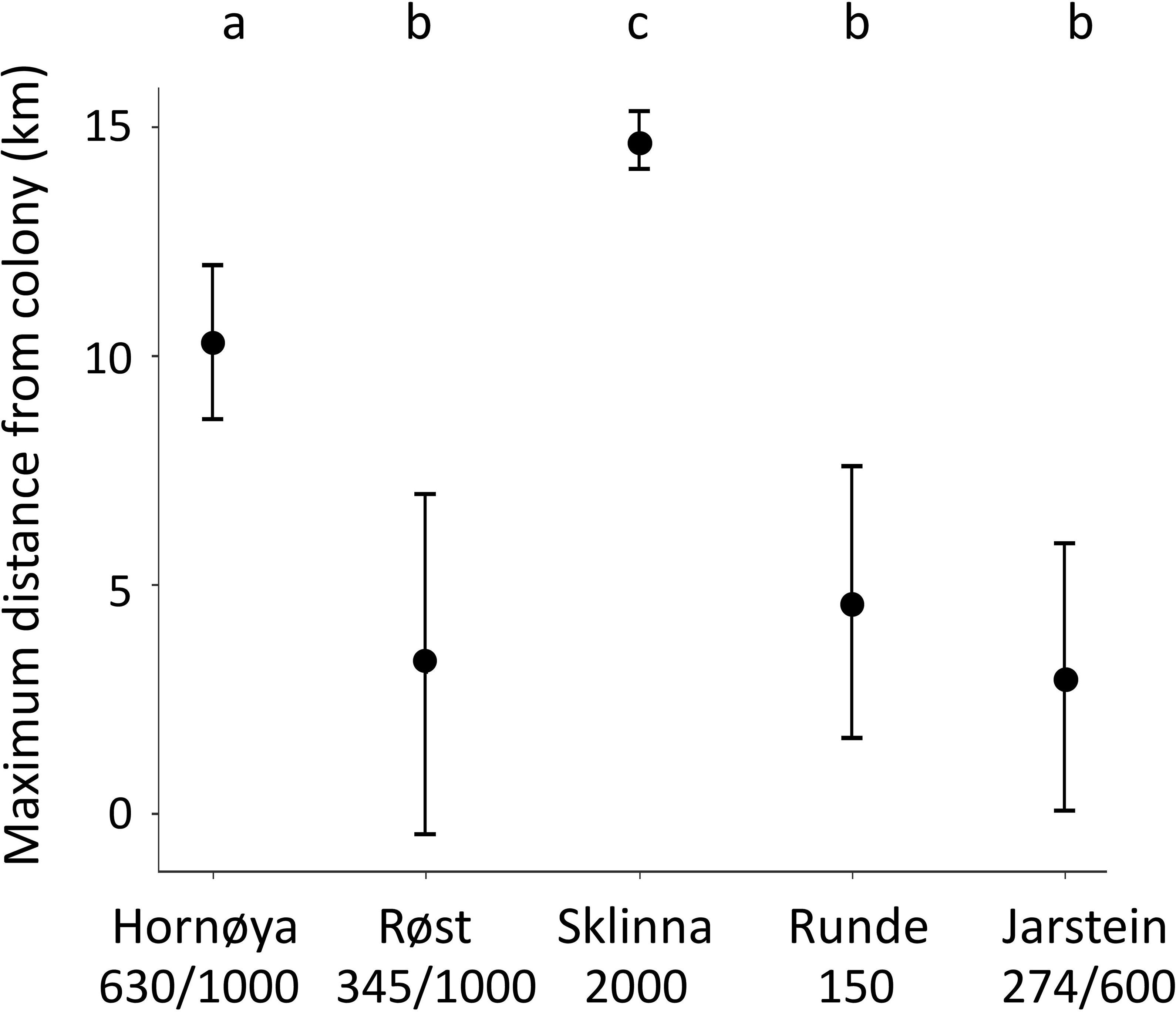
Figure 2 Predicted values of foraging range between the five study colonies based on the LMM results (mean ± CI). Only complete foraging trips were considered. Letters at the top correspond to the results of Tukey post-hoc tests based on the LMM (see Methods and Material). Different letters indicate strong evidence for colony-specific differences in foraging range (all z ≥ 3.4; P ≤ 0.005), same letters indicate no evidence for such differences (all z ≤ 0.773, P ≥ 0.930). Colony sizes (number of breeding pairs) are given below the colony names. Numbers behind the dash (/) give the approximate total number of breeding pairs within the maximum foraging range of the focal colony, in case of neighbouring colonies.
Environmental Habitat Preferences Per Colony
Across colonies, depth or distance to colony were the single best explanatory environmental variables and explained alone at least 22% of deviance (Table 2). Both were supported in the final model for all colonies except Røst, where depth correlated with distance to colony and therefore only distance to colony was included in the final model (Table 2). The probability for foraging declined steeply in all colonies with increasing depth (Figure 3A) and approached zero for all colonies at a depth of 100 m or more. The probability for foraging also declined steeply with increasing distance from colony (Figure 3B), and approached zero at a distance of 10 km for birds from Røst and Runde. Birds from Sklinna showed a second peak in foraging probability at 20 km distance, and similarly for Hornøya there was a slight increase at this distance.
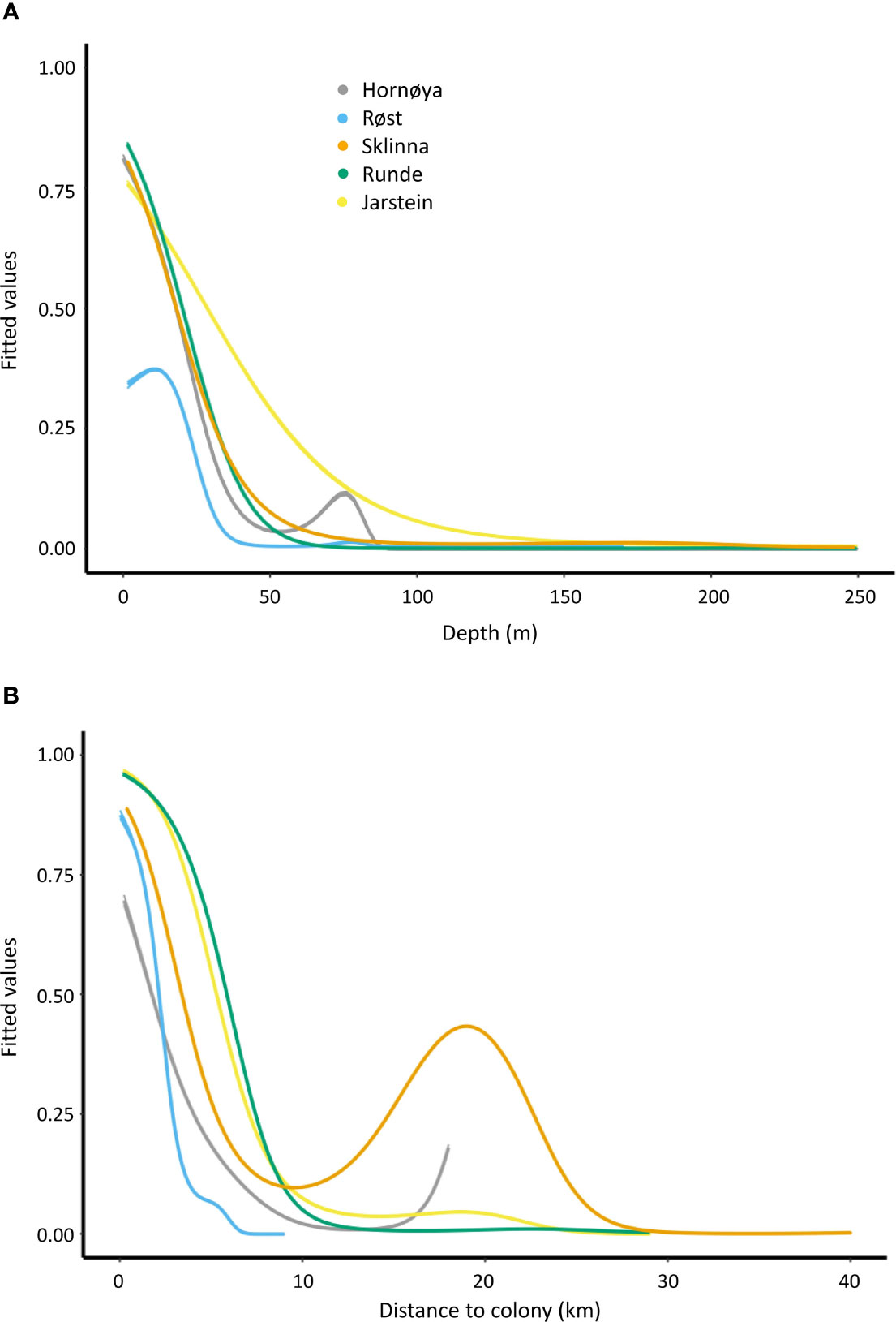
Figure 3 Model response curves (fitted values ± SE) showing the predicted foraging probability in response to depth (A) and distance from colony (B) for the different colonies. Fitted values were extracted from the individual models per colony (e.g. for the Hornøya colony model HM3 and HM5; see Table 3).
The inclusion of kelp was supported in the final models for all colonies (Table 2). There was very strong evidence that the presence of kelp increased the foraging probability of shags at all colonies except at Hornøya (z-values ≥ 16.16, p < 0.001 in the best models for Røst, Sklinna, Runde and Jarstein; Hornøya: z = 0.128, p = 0.898). In addition, ssh mean was included in the final models for Sklinna, Hornøya and Jarstein, and ssh variance in the models for Røst and Runde. However, by adding ssh to the models, the adjusted R2 value increased by at maximum 0.05 (Table 2), reflecting a relatively minor importance of ssh for the characterisation of shag foraging habitat. The final models explained between 53.5% and 81.5% of the deviance, reflecting a good to very good fit (Table 2).
Transferability Within and Across Colonies
Transferability across years within the same colony was highly variable and ranged between 0.50 and 0.98, when both the training and the testing dataset consisted of data from one year each (Supplement 3). Transferability across years at Sklinna was considerably higher for all years when the training dataset consisted of nine years of data, i.e. all years except the testing year (AUC range: 0.96-0.98) compared to when the training dataset consisted of one year only (AUC range: 0.51-0.98).
Following the “individual colony and year approach” (i.e. both the training and the testing dataset consisted of the data from one colony and one year each), transferability across colonies was variable and ranged between 0.45 and 0.99, with an average AUC of 0.73 ± 0.11 (Supplement 3). Thus, predictability could be excellent in some cases (e.g. using the Jarstein 2019 data to predict the foraging locations of birds at Runde in 2020, with an AUC of 0.99; see Supplement 3), or poor in other cases (e.g. data from Røst 2020 predicting the foraging locations of birds at Hornøya in 2011, with an AUC of 0.46; Supplement 3).
With the “individual colony approach” (i.e. the training and the testing dataset consisted of all data from all years of a given colony), the transferability across colonies remained highly variable (AUC ranged between 0.36 to 0.98, mean 0.76 ± 0.16; Table 3). For example, Jarstein was poor in predicting the foraging locations for all colonies but Runde. The Sklinna dataset, on the other hand, predicted the foraging locations at all other colonies comparatively well (AUC range of 0.85-0.98). Transferability was not necessarily higher between colonies located closer to each other, e.g. transferability was better from Røst to Runde and Jarstein, than from Røst to Hornøya and Sklinna, and transferability from Runde to Jarstein was the lowest overall (Figure 1, Table 3).
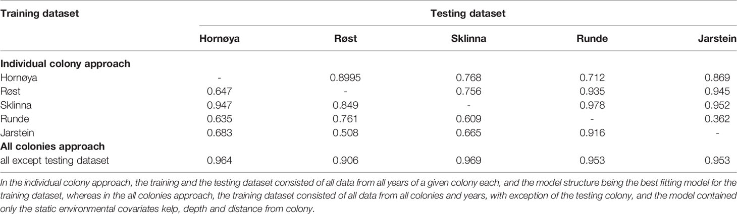
Table 3 AUC results of models based on the individual colonies approach (top) and the all colonies approach (below).
Finally, with the “all colonies approach” (i.e. the training dataset consisted of all data from all colonies and years, with exception of the testing colony), transferability across colonies was highest and least variable (AUC range: 0.91-0.97; Table 3). The prediction maps based on this final model highlighted the shallow, near-shore areas as the most important foraging habitat for the shags (Figure 4). The foraging locations based on the GPS tracking data were mostly located within the predicted areas, although foraging locations were often closer to the colonies than the range predicted by the models (Figure 4).
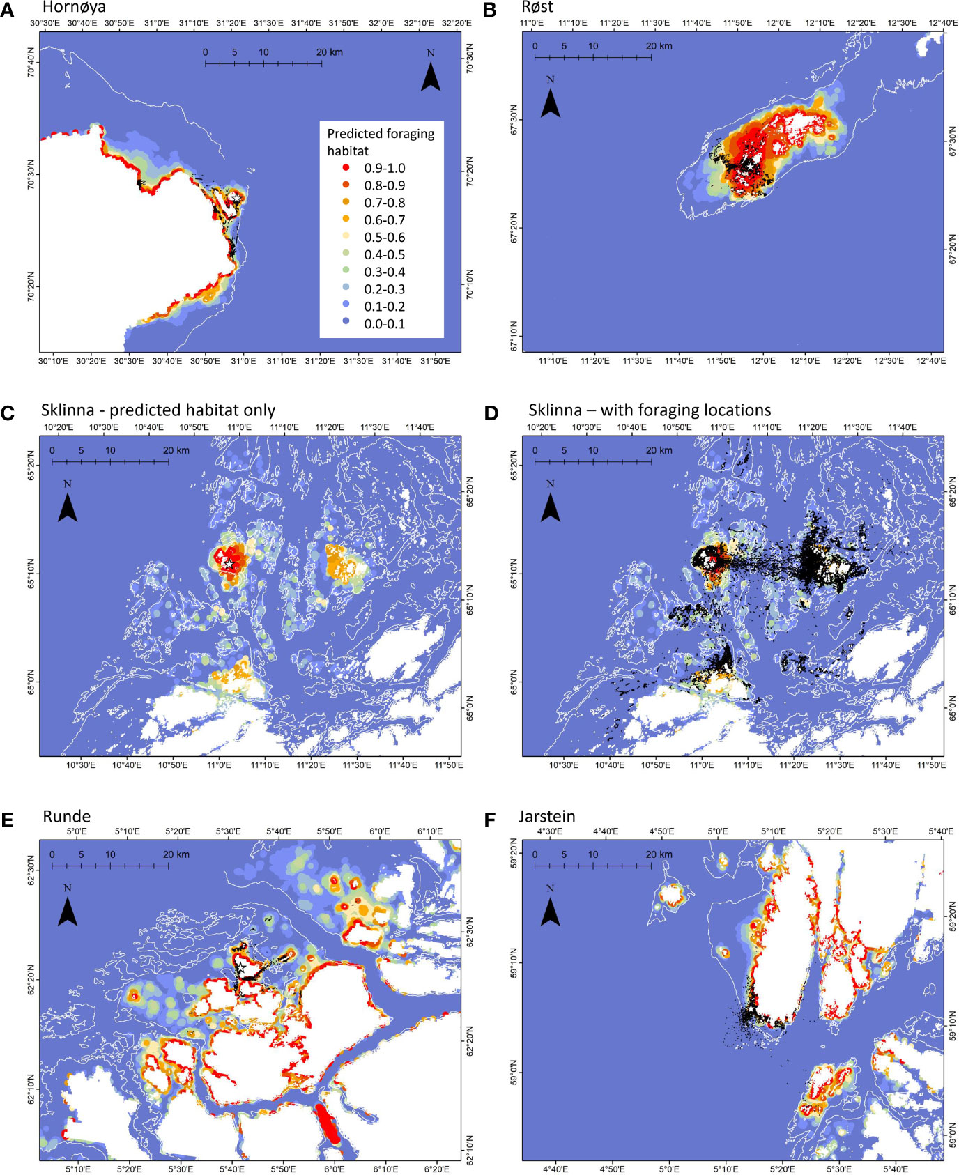
Figure 4 Predicted habitat maps based on the “all colonies approach” models, i.e. data from all other colonies and years was used to predict the foraging habitat around the shown (focal) colony. The location of the colony is marked with a white star. The probability for the area to be used as foraging habitat is shown in colours from blue (low) to red (high), as detailed in the legend. White lines show the 100m bathymetry line, land areas are depicted in white. Foraging locations based on the EMBC algorithm are shown as black dots (A, B, D–F). Due to the high data amount, foraging locations for Sklinna are shown in a separate plot (D) than the predicted foraging habitat (C).
Discussion
Environmental Habitat Preferences
As expected, we found that distance to colony, depth and the presence of kelp were the most important variables to characterise foraging habitat across all colonies. Sea surface temperature (sst) was not supported in the final models to characterise foraging habitat, while sea surface height (ssh) was supported in the models, but was of comparatively minor importance.
As expected for a benthic diving species, models suggested that foraging activity increased with shallower depth. This also matched with the dive data obtained in this study, with average dive depths at all colonies being in the range of 7-13 m, and no dive being deeper than 63 m (Table S1.2, Supplement 1). Further, matching our prediction, foraging probability increased in the presence of kelp. Only at Hornøya could we not find evidence for shag foraging activity increasing in the presence of kelp forests, although kelp was still supported as a factor in the models. Kelp forests, with Laminaria hyperborea being the dominating species, typically occur in water depths down to 30 m depth, and on rocky substrate (Bekkby et al., 2009), thus not all shallow marine habitats are colonised by kelp. Around Hornøya and many other areas in northern Norway, kelp forests are very sparce or absent after a collapse in the 1970s and 1980s due to overgrazing by the green sea urchin (Strongylocentrotus droebachiensis) (Christie et al., 2019). As such, only 8% of the likely foraging locations around Hornøya were associated with the presence of kelp, compared to 51% in the other colonies. The low availability of kelp forests thus likely explained the lower importance of this habitat type for Hornøya compared to the other colonies. Our results are – not surprisingly – in agreement with earlier studies from Norway (based partly on the same GPS data), showing that kelp forests are of high importance around Sklinna, while data for kelp presence was lacking until recently for the area around Hornøya and could thus not be included into earlier analyses (Christensen-Dalsgaard et al., 2017). Depth, on the other hand, was of importance at both Sklinna and Hornøya also in the previous study (Christensen-Dalsgaard et al., 2017), and in Normandy, France (Grémillet et al., 2020), where shags in fact used much shallower habitats with an apparent preference at about 10 m depth. In distribution models for shags around the British Isles, depth was not retained as important variable, possibly due to the coarser spatial scale of the models, and the inclusion of non-foraging locations (Wakefield et al., 2017). In contrast, and in agreement with our results, in an analysis of habitat use by shags around the Isle of May, Scotland, shags tended to avoid areas with water depths exceeding 60m (Daunt et al., 2012).
The lack of importance of sst and ssh parameters to characterise foraging locations of shags is maybe less surprising given the benthic foraging behaviour of this species and thus the strong preference for shallow foraging areas. Instead of indicating distinctions in water masses and thus frontal zones, eddies or upwelling plumes, respectively (e.g. Kostianoy et al., 2004; Ainley et al., 2009; Mason et al., 2014), we found mean sst and mean ssh but also temporal variance in sst and ssh to increase from pelagic towards coastal habitats, reaching highest levels in near-shore areas (Supplement 2). Sea surface temperatures also reflected the negative trend towards lower temperatures with increasing latitude. Furthermore, both mean sst and mean ssh showed some annual variation, with distinct gradients in the coastal zones in some but not all years (Supplement 2). Quite possibly, the variation across years also contributed to lower across-year and across-colony transferability of models containing ssh. Sea surface height and sst, albeit retained in models, also seemed to be of lower importance for shags in Normandy (Grémillet et al., 2020) and in the British Isles (sst only; Wakefield et al., 2017).
Besides the environmental covariates, distance to colony was an important variable in the models for all colonies. This is in agreement with the study by Wakefield et al. (2017), who found distance to colony as well as the number of conspecific breeders to be of strong importance in shag distribution models. In accordance with this, we found foraging range to be largest for the biggest colony, Sklinna with 2000 breeding pairs, where shags foraged up to 40 km away from their breeding location, and smallest at Røst, with 345 breeding pairs in the study colony (and approximately 1000 pairs in the entire 20 x10 km² archipelago), where foraging occurred within a radius of 9 km from the colony. However, given the size of our dataset (only 5 colonies) and uncertainty about colony sizes in the direct vicinity of our study colonies, we did not test for a relationship between colony size and foraging range.
Transferability Within and Across Colonies
Transferability of foraging habitats across colonies differed depending on which of the three modelling approaches was used. With the individual colony and year approach, transferability was overall low, and the results in many instances unsatisfactory. The individual colony and year approach was also used to assess transferability across years within colonies. Even within the same colony, the transferability was poor across years. Noteworthy, transferability was low across colonies and years, and thus not an artefact of few individuals tracked (or a low number of foraging trips recorded) at a given colony in a given year (cf. between-year transferability based on Hornøya 2011 data (AUC = 0.552; N = 31 individuals, 157 complete trips) and Sklinna 2014 data (AUC = 0.608-0.954; average: 0.772; N = 55 individuals, 167 complete trips) being very low compared to the high across-year transferability based on the Røst 2020 data (AUC = 0.908; N = 7 individuals, 42 complete trips). While transferability across years within the same colony was on average in the same range as for across-year transferability of breeding season habitat of Scopoli’s shearwaters (Calonectris diomedea; Péron et al., 2018), we had more extreme values to both ends. Transferability across years increased substantially for the Sklinna dataset when nine years of data were used in the training dataset, to predict the habitat use in the tenth year. Unfortunately, given that we only had two years of tracking data at all other colonies, we could not test if this pattern was universal.
With transferability across years within the same colony being limited when the training dataset consisted of only one year, it was not surprising to also find low transferability across colonies. In a management perspective, using the tracking data from only one year and one colony to predict habitat use by birds around another colony, increases the risk of focussing on an area that is of only minor importance, and – worse – not protecting the really important habitat.
The individual colony approach yielded slightly better outcomes regarding the transferability across colonies than the individual colony and year approach. Thus, pooling the data from each colony together in the training dataset helped to improve predictability. However, the results were still variable. Against our expectation, and in contrast to previous findings (Péron et al., 2018; Fauchald et al., 2021), transferability across colonies was not higher for those colonies being relatively more closely located. Thus, the dataset from Runde was poor to predict foraging habitat characteristics at either Sklinna (located 400 km away) or Jarstein (located 360 km away), while the Hornøya dataset was good in predicting the foraging habitat characteristics at both Runde (1420 km away) and Jarstein (1730 km away). Possibly, the actual distances between our study colonies (all ≥ 250 km) were still too large to allow good transferability at a high spatial scale. In fact they were larger than for those colonies with good transferability in the work by Péron et al. (2018) on breeding Scopoli’s shearwaters. Although Fauchald et al. (2021) found high transferability of winter distribution for colonies located less than 500 km away from each other, seabirds are much less restricted in habitat use during winter than during the breeding season (Bell, 1990), and their study was also based on six pelagic seabird species, and not coastal-bound shags. Rather than relative proximity between colonies playing a role for transferability, similarity of foraging habitat between specific colonies, or availability of prey may be factors affecting transferability. Shags are fish specialists, and availability of fish is obviously a key determinant of where and what shags are feeding. Unfortunately, we do not have a complete overview of the diet for all of our study colonies, but there is some clear variation between the colonies: Young age classes of saithe (Pollachius virens) are the dominating prey at Sklinna and Røst (Hillersøy and Lorentsen, 2012; Lorentsen et al., 2018; Anker-Nilssen unpublished data), whereas lesser sandeel (Ammodytes marinus) is the main prey, followed by gadoids, including saithe, at Hornøya (Barrett et al., 1990). Shags at Runde fed on a mix of gadoids, including saithe as well as sandeel (Graham, 2019), while we had no diet information from Jarstein. Based on the diet, one could thus have expected higher transferability between Sklinna and Røst as well as between Hornøya and Runde, but poorer transferability between Sklinna and Hornøya, Sklinna and Runde, Røst and Hornøya, as well as Røst and Runde, respectively. Evidence for this was rather mixed, though (Table 2).
Overall, it rather seemed that some datasets were better to train models than others, which was the case particularly for the Sklinna dataset. This again may not be too surprising given that Sklinna was the only colony for which we had more than 2 years of data, and many more individuals were tracked in this colony than from other colonies. The importance of multi-year tracking of shags to capture the full range of utilised habitats has been highlighted earlier by Bogdanova et al. (2014). In addition, shags are known to show individual segregation in foraging space use (Morgan et al., 2019), and thus a dataset that holds multiple foraging trips from more individuals likely covers a wider range of environmental habitats than the same number of trips obtained from fewer individuals (as e.g. for the Røst 2020 dataset). The Sklinna dataset was therefore in a way more diverse and the large foraging range at this colony in addition to the 10 years of tracking may have contributed to covering a broader range of environmental variables than at other colonies, possibly making this dataset more suitable for predictions.
Finally, the all colonies approach, i.e. the approach based only on the temporally static environmental variables (depth, distance and kelp), and pooling all data from all colonies except for the testing colony, performed best and transferability across colonies was very high for all five colonies. This high performance may have several non-exclusive reasons: Firstly, dropping the spatio-temporally variable covariates ssh mean and ssh variance and only including temporally stable environmental covariates into the training model may have improved transferability. At individual colonies it was either ssh mean or ssh variance that was supported in the models. As such, including e.g. ssh mean in a model when predicting the utilised habitat at a colony for which ssh variance was supported (as was the approach in the individual colony and year approach and the individual colonies approach) would in fact likely not improve model fit and thus transferability. In this context, it is further noteworthy that ssh mean and ssh variance, even though supported in the models to characterise foraging habitats, were of generally lower importance than the temporally non-variable environmental covariates (i.e. depth, distance to colony and kelp presence) that remained included in the models of the all colonies approach. Secondly, using a very diverse training dataset, consisting of four colonies with at least 2 years of data each, very likely also contributed to improving model fit and transferability of the results from one colony to another. This would be a similar effect as discussed above as a possible reason for why the Sklinna dataset in the individual colony approach performed best to predict utilised habitat in all other colonies, and also why within-colony transferability increased for Sklinna when the training dataset contained nine years instead of only one. Importantly, while Sklinna performed well as a training dataset with the individual colony approach, the data from the other colonies performed on average poorly to predict the utilised habitat of the shags around Sklinna. In contrast, with the all colonies approach, the utilised habitat was predicted very well also around Sklinna. Therefore, our results clearly highlight that with a solid database, consisting of at least 2 years of tracking data from several different colonies, it is possible to predict important habitat around another shag colony – even when working across large spatial scales.
It remains open to which degree our data can be used to predict the foraging hot-spots of shags in other parts of their breeding range, and we advocate strongly against blindly predicting key foraging habitat outside of Norway based on our data. Shags are geographically widespread and as pointed out above, variability in diet across colonies as well as availability of habitat around colonies contribute to differences in foraging habitat use. Despite the variable diet across the colonies, we were able to predict the habitat use of shags at all colonies with high precision with our complete dataset. Possibly, this was helped by the comparatively similar bathymetry along the Norwegian coastline, with relatively shallow zones near-shore along the coast (around the often many islands and skerries) inside of a much deeper continental shelf. However, our models may not function equally well in areas with other habitat compositions, for example if all available habitat around a colony was characterised by comparatively shallow sandy bottom as was the case in Normandy (Grémillet et al., 2020).
Conclusions
Our in-depth analyses of habitat use of shags in five different colonies along the Norwegian coast reflects the importance of collecting data over several years and in several colonies, and shows the value of comprehensive datasets in modelling and predicting important foraging areas. Our study is the first to test transferability of fine-scale habitat models in shags, and the first study assessing transferability of habitat models across colonies based on different approaches. Our dataset and modelling approach puts us in the unique position to be able to predict important foraging habitat around any shag colony along the Norwegian coast, likely with a reasonably high level of accuracy, without the need to track birds in additional colonies. Our models on foraging habitat included distance to colony, thus the transferred predictions sometimes highlighted areas as important that were further away from the colony than those used by the tracked birds (cf. Figure 4). This will require some more fine-tuning of predictions about the foraging range around colonies, possibly by combining our method with the foraging radius approach as part of the BirdLife International (2010) toolbox, or using also the relationship between colony size and foraging range, as successfully performed by Wakefield et al. (2017).
Shags have or are experiencing population declines in most parts of their distribution range (BirdLife International, 2021). In Norway, population sizes showed substantial inter-decadal variation over the past 40 years, and a regional decline in the Barents Sea, while the overall population number appears relatively stable (Fauchald et al., 2015). With about 35% of the NE Atlantic population (Mitchell et al., 2004), Norway has a special responsibility for the conservation of shags. Consequently, information on the most suitable foraging areas for shags should always be at hand for management authorities to consider proper measures when anthropogenic pressures have the potential to substantially reduce their quality as foraging habitat or hinder birds access to such areas.
The UN decided in 2015 that, by 2030, 30% of the marine environment, including coastal zones, should be protected. We are, however, still far from reaching that goal, both globally, regionally (Europe and North America) and nationally (Maestro et al., 2019). This is also true for Norway, which by 2020 had only protected 3.5% of its territorial waters (Statistics Norway, 2021). On the contrary, Norway’s coastal industries like fisheries and, in particular, aquaculture are expected to increase fivefold by 2050 (Olafsen et al., 2012), including plans for opening of additional, large areas to kelp harvesting (Steen et al., 2020). In such times of increasing anthropogenic pressures on coastal marine habitats and the rising need for better management of wildlife, our work delivers important knowledge for ecosystem-based management decisions, which could contribute to reach the UN goals for 2030.
Data Availability Statement
The raw data supporting the conclusions of this article will be made available by the authors, without undue reservation.
Ethics Statement
The animal study was reviewed and approved by The Norwegian Food Safety Authority (Mattilsynet).
Author Contributions
Conceptualization: SC-D and S-HL. Funding acquisition and project management: SC-D. Data were collected by ND, TA-N, S-HL, and SC-D. Analyses were completed by ND, with contributions from JM, and AT. Writing was led by ND, with contributions from all other authors. All authors contributed to the article and approved the submitted version.
Funding
This study was part of the SEAPOP programme (www.seapop.no/en), which is financed by the Norwegian Ministry of Climate and Environment via the Norwegian Environment Agency, the Norwegian Ministry of Petroleum and Energy via the Norwegian Research Council (grant 192141), and the Norwegian Oil and Gas Association.
Conflict of Interest
The authors declare that the research was conducted in the absence of any commercial or financial relationships that could be construed as a potential conflict of interest.
Publisher’s Note
All claims expressed in this article are solely those of the authors and do not necessarily represent those of their affiliated organizations, or those of the publisher, the editors and the reviewers. Any product that may be evaluated in this article, or claim that may be made by its manufacturer, is not guaranteed or endorsed by the publisher.
Acknowledgments
Thanks to the many field assistants for helping to deploy and retrieve GPS and TDR loggers, especially Oskar Bjørnstad, Hans Inge Hansen and Ingar Støyle Bringsvor. Thanks also to Jon Albretsen at the Norwegian Institute of Marine Research for providing SST and SSH data and answering related questions, and to Ute Bradter for help with R-coding. We obtained permits to work in the colonies from the local County governors, permissions to catch birds and attach loggers from the Environmental Agency and The Norwegian Food Safety Authority. The Norwegian Coastal Administration facilitated extended stays at several of the colonies through rental agreements for the lighthouse stations.
Supplementary Material
The Supplementary Material for this article can be found online at: https://www.frontiersin.org/articles/10.3389/fmars.2022.852033/full#supplementary-material
References
Aarts G., MacKenzie M., McConnell B., Fedak M., Matthiopoulos J. (2008). Estimating Space-Use and Habitat Preference From Wildlife Telemetry Data. Ecography 31, 140–160. doi: 10.1111/j.2007.0906-7590.05236.x
Ainley D. G., Dugger K. D., Ford R. G., Pierce S. D., Reese D. C., Brodeur R. D., et al. (2009). Association of Predators and Prey at Frontal Features in the California Current: Competition, Facilitation, and Co-Occurrence. Mar. Ecol. Prog. Ser. 389, 271–294. doi: 10.3354/meps08153
Albretsen J., Sperrevik A. K., Staalstrøm A., Sandvik A. D., Vikebø F., Asplin L. (2011). “NorKyst-800 Report No. 1 User Manual and Technical Descriptions,” in Fisken og Havet 2 (Bergen, Norway: Havforskningsinstituttet - Institute of Marine Research).
Anderson O. R. J., Small C. J., Croxall J. P., Dunn E. K., Sullivan B. J., Yates O., et al. (2011). Global Seabird Bycatch in Longline Fisheries. End. Spec. Res. 14, 91–106. doi: 10.3354/esr00347
Asplin L., Albretsen J., Johnsen I. A., Sandvik A. D. (2020). The Hydrodynamic Foundation for Salmon Lice Dispersion Modeling Along the Norwegian Coast. Ocean. Dyn. 70, 1151–1167. doi: 10.1007/s10236-020-01378-0
Barrett R. T., Røv N., Loen J., Montevecchi W. A. (1990). Diets of Shags Phalacrocorax Aristotelis and Cormorants P. Carbo in Norway and Possible Implications for Gadoid Stock Recruitment. Mar. Ecol. Prog. Ser. 66, 205–218. doi: 10.3354/meps066205
Bates D., Maechler M., Bolker B. (2015). Fitting Linear Mixed-Effects Models Using Lme4. J. Stat. Softw. 67, 1–48. doi: 10.18637/jss.v067.i01
Bekkby T., Rinde E., Erikstad L., Bakkestuen V. (2009). Spatial Predictive Distribution Modelling of the Kelp Species Laminaria Hyperborea. ICES J. Mar. Sci. 66, 2106–2115. doi: 10.1093/icesjms/fsp195
Bell W. J. (1990). “Central Place Foraging”, in Searching Behaviour: The Behavioural Ecology of Finding Resources (Dordrecht, the Netherlands: Springer). doi: 10.1007/978-94-011-3098-1_12
Beveridge M. C. M. (2001). “Aquaculture and Wildlife Interactions”, in Environmental Impact Assessment of Mediterranean Aquaculture Farms. Eds. Uriarte A., Basurco B. (Zaragoza: CIHEAM: Cahiers Options Méditerranéennes), 57–66.
BirdLife International (2010). Marine Important Bird Areas Toolkit: Standardised Techniques for Identifying Priority Sites for the Conservation of Seabirds at Sea (Cambridge UK: BirdLife International). Version 1.2: February 2011.
BirdLife International (2016) Summary of National Hunting Regulations (Norway). Available at: http://datazone.birdlife.org/userfiles/file/hunting/HuntingRegulations_Norway.pdf (Accessed December 1, 2021).
BirdLife International (2021) Species Factsheet: Gulosus Aristotelis. Available at: http://www.birdlife.org (Accessed December 1, 2021).
Bivand R. S., Pebesma E., Gomez-Rubio V. (2013). Applied Spatial Data Analysis With R. 2nd ed. (New York: Springer).
Bogdanova M. I., Wanless S., Harris M. P., Lindström J., Butler A., Newell M. A., et al. (2014). Among-Year and Within-Population Variation in Foraging Distribution of European Shags Phalacrocorax Aristotelis Over Two Decades: Implications for Marine Spatial Planning. Biol. Conserv. 170, 292–299. doi: 10.1016/j.biocon.2013.12.025
Brown E. J., Vasconcelos R. P., Wennhage H., Bergström U., Støttrup J. G., van de Wolfshaar K., et al. (2018). Conflicts in the Coastal Zone: Human Impacts on Commercially Important Fish Species Utilizing Coastal Habitat. ICES J. Mar. Sci. 75, 1203–1213. doi: 10.1093/icesjms/fsx237
Burnham K. P., Anderson D. R. (2002). Model Selection and Multimodel Interference. A Practical Information-Theoretic Approach (New York: Springer).
Cecere J. G., De Pascalis F., Imperio S., Ménard D., Catoni C., Griggio M., et al. (2020). Inter-Individual Differences in Foraging Tactics of a Colonial Raptor: Consistency, Weather Effects, and Fitness Correlates. Mov. Ecol. 8, 28. doi: 10.1186/s40462-020-00206-w
Christensen-Dalsgaard S., Anker-Nilssen T., Crawford R., Bond A., Sigurðsson G. M., Glemarec G., et al. (2019). What’s the Catch With Lumpsuckers? A North Atlantic Study of Seabird Bycatch in Lumpsucker Gillnet Fisheries. Biol. Conserv. 240, 108278. doi: 10.1016/j.biocon.2019.108278
Christensen-Dalsgaard S., Mattisson J., Bekkby T., Gundersen H., May R., Rinde E., et al. (2017). Habitat Selection of Foraging Chick-Rearing European Shags in Contrasting Marine Environments. Mar. Biol. 164, 196. doi: 10.1007/s00227-017-3227-5
Christensen-Dalsgaard S., Mattisson J., Norderhaug K. M., Lorentsen S.-H. (2020). Sharing the Neighbourhood: Assessing the Impact of Kelp Harvest on Foraging Behaviour of the European Shag. Mar. Biol. 167, 136. doi: 10.1007/s00227-020-03739-1
Christie H., Gundersen H., Rinde E., Filbee-Dexter K., Norderhaug K. M., Pedersen T., et al. (2019). Can Multitrophic Interactions and Ocean Warming Influence Large-Scale Kelp Recovery? Ecol. Evol. 9, 2847–2862. doi: 10.1002/ece3.4963
Craik C. (1997). Long-Term Effects of North American Mink Mustela Vison on Seabirds in Western Scotland. Bird Study 44, 303–309. doi: 10.1080/00063659709461065
Crain C. M., Kroeker K., Halpern B. S. (2008). Interactive and Cumulative Effects of Multiple Human Stressors in Marine Systems. Ecol. Lett. 11, 1304–1315. doi: 10.1111/j.1461-0248.2008.01253.x
Cramp S., Simmons K. E.. (1977). The Birds of the Western Palearctic. Handbook of the Birds of Europe, the Middle East and North Africa, Vol I. Ostrich to Ducks. Oxford University Press, Oxford, U.K.
Cury P. M., Boyd I. L., Bonhommeau S., Anker-Nilssen T., Crawford R. J. M., Furness R. W., et al. (2011). Global Seabird Response to Forage Fish Depletion - One-Third for the Birds. Science 334, 1703–1706. doi: 10.1126/science.1212928
Daunt F., Afanasyev V., Adam A., J P C., Wanless S. (2007). From Cradle to Early Grave: Juvenile Mortality in European Shags Phalacrocorax Aristotelis Results From Inadequate Development of Foraging Proficiency. Biol. Lett. 3, 371–374. doi: 10.1098/rsbl.2007.0157
Daunt F., Bogdanova M., McDonald C., Wanless S. (2012). “Determining Important Marine Areas Used by European Shag Breeding on the Isle of May That Might Merit Consideration as Additional SPAs,” in JNCC Report No 556 (Peterborough, UK: Joint Nature Conservation Committee JNCC).
Davies T. E., Carneiro A. P. B., Campos B., Hazin C., Dunn D. C., Gjerde K. M., et al. (2021). Tracking Data and the Conservation of the High Seas: Opportunities and Challenges. J. Appl. Ecol. 58, 2703–2710. doi: 10.1111/1365-2664.14032
Dehnhard N., Achurch H., Clarke J., Michel L. N., Southwell C., Sumner M. D., et al. (2020b). High Inter- and Intraspecific Niche Overlap Among Three Sympatrically Breeding, Closely Related Seabird Species: Generalist Foraging as an Adaptation to a Highly Variable Environment? J. Anim. Ecol. 89, 104–119. doi: 10.1111/1365-2656.13078
Dehnhard N., Skei J., Christensen-Dalsgaard S., May R., Halley D., Ringsby T. H., et al. (2020a). Boat Disturbance Effects on Moulting Common Eiders Somateria Mollissima. Mar. Biol. 167, 12. doi: 10.1007/s00227-019-3624-z
De Pascalis F., Imperio S., Benvenuti A., Catoni C., Rubolini D., Cecere J. G. (2020). Sex-Specific Foraging Behaviour is Affected by Wind Conditions in a Sexually Size Dimorphic Seabird. Anim. Behav. 166, 207–218. doi: 10.1016/j.anbehav.2020.05.014
Dias M. P., Martin R., Pearmain E. J., Burfield I. J., Small C., Phillips R. A., et al. (2019). Threats to Seabirds: A Global Assessment. Biol. Conserv. 237, 525–537. doi: 10.1016/j.biocon.2019.06.033
Edgar G. J., Stuart-Smith R. D., Willis T. J., Kininmonth S., Baker S. C., Banks S., et al. (2014). Global Conservation Outcomes Depend on Marine Protected Areas With Five Key Features. Nature 506, 216–220. doi: 10.1038/nature13022
Evans J. C., Dall S. R. X., Bolton M., Owen E., Votier S. C. (2016). Social Foraging European Shags: GPS Tracking Reveals Birds From Neighbouring Colonies Have Shared Foraging Grounds. J. Ornithol. 157, 23–32. doi: 10.1007/s10336-015-1241-2
Fauchald P., Anker-Nilssen T., Barrett R. T., Bustnes J. O., Bårdsen B. J., Christensen-Dalsgaard S., et al. (2015). “The Status and Trends of Seabirds Breeding in Norway and Svalbard,” in NINA Report 1151 (Tromsø, Norway: Norwegian Institute for Nature Research).
Fauchald P., Tarroux A., Amélineau F., Bråthen V. S., Descamps S., Ekker M., et al. (2021). Year-Round Distribution of Northeast Atlantic Seabird Populations: Applications for Population Management and Marine Spatial Planning. Mar. Ecol. Prog. Ser. 676, 255–276. doi: 10.3354/meps13854
Furness R. W., Wade H., Masden E. (2013). Assessing Vulnerability of Seabird Populations to Offshore Wind Farms. J. Environ. Manag. 119, 56–66. doi: 10.1016/j.jenvman.2013.01.025
Garriga J., Palmer J. R. B., Oltra A., Bartumeus F. (2016a). “EMbC: Expectation-Maximization Binary Clustering,” in R package version 1.9.4. Available at: https://CRAN.R-project.org/package=EMbC.
Garriga J., Palmer J. R. B., Oltra A., Bartumeus F. (2016b). Expectation-Maximization Binary Clustering for Behavioural Annotation. PLoS One 11, e0151984. doi: 10.1371/journal.pone.0151984
Garthe S., Hüppop O. (2004). Scaling Possible Adverse Effects of Marine Wind Farms on Seabirds: Developing and Applying a Vulnerability Index. J. Appl. Ecol. 41, 724–734. doi: 10.1111/j.0021-8901.2004.00918.x
Graham L. K. (2019). A Pilot Study Assessing Drones for Mapping and Monitoring of European Shags (Trondheim: Master Thesis, Norwegian University of Science and Technology).
Grémillet D., Boulinier T. (2009). Spatial Ecology and Conservation of Seabirds Facing Global Climate Change: A Review. Mar. Ecol. Prog. Ser. 391, 121–137. doi: 10.3354/meps08212
Grémillet D., Gallien F., El Ksabi N., Courbin N. (2020). Sentinels of Coastal Ecosystems: The Spatial Ecology of European Shags Breeding in Normandy. Mar. Biol. 167, 43. doi: 10.1007/s00227-020-3655-5
Halpern B. S., Frazier M., Potapenko J., Casey K. S., Koenig K., Longo C., et al. (2015). Spatial and Temporal Changes in Cumulative Human Impacts on the World’s Ocean. Nat. Comm. 6, 7615. doi: 10.1038/ncomms8615
Hijmans R. J. (2021). “Raster: Geographic Data Analysis and Modeling,” in R package version 3.4-13. Available at: https://CRAN.R-project.org/package=raster.
Hillersøy G., Lorentsen S.-H. (2012). Annual Variation in the Diet of Breeding European Shag (Phalacrocorax Aristotelis) in Central Norway. Waterbirds 35, 420–430. doi: 10.1675/063.035.0306
Hothorn T., Bretz F., Westfall P. (2008). Simultaneous Inference in General Parametric Models. Biometric J. 50, 346–363. doi: 10.1002/bimj.200810425
Howells R. J., Burthe S. J., Green J. A., Harris M. P., Newell M. A., Butler A., et al. (2018). Pronounced Long-Term Trends in Year-Round Diet Composition of the European Shag Phalacrocorax Aristotelis. Mar. Biol. 165, 188. doi: 10.1007/s00227-018-3433-9
Jovani R., Lascelles B., Garamszegi L. Z., Mavor R., Thaxter C. B., Oro D. (2016). Colony Size and Foraging Range in Seabirds. Oikos 125, 968–974. doi: 10.1111/oik.02781
Keogan K., Daunt F., Wanless S., Phillips R. A., Walling C. A., Agnew P., et al. (2018). Global Phenological Insensitivity to Shifting Ocean Temperatures Among Seabirds. Nat. Clim. Change 8, 313. doi: 10.1038/s41558-018-0115-z
Kostianoy A. G., Ginzburg A. I., Frankignoulle M., Delille B. (2004). Fronts in the Southern Indian Ocean as Inferred From Satellite Sea Surface Temperature Data. J. Mar. Sys. 45, 55–73. doi: 10.1016/j.jmarsys.2003.09.004
Lascelles B. G., Taylor P. R., Miller M. G. R., Dias M. P., Oppel S., Torres L., et al. (2016). Applying Global Criteria to Tracking Data to Define Important Areas for Marine Conservation. Div. Dist. 22, 422–431. doi: 10.1111/ddi.12411
Lorentsen S. H., Anker-Nilssen T., Erikstad K. E. (2018). Seabirds as Guides for Fisheries Management: European Shag Phalacrocorax Aristotelis Diet as Indicator of Saithe Pollachius Virens Recruitment. Mar. Ecol. Prog. Ser. 586, 193–201. doi: 10.3354/meps12440
Lorentsen S. H., Mattisson J., Christensen-Dalsgaard S. (2019). Reproductive Success in the European Shag is Linked to Annual Variation in Diet and Foraging Trip Metrics. Mar. Ecol. Prog. Ser. 619, 137–147. doi: 10.3354/meps12949
Lorentsen S. H., Sjøtun K., Grémillet D. (2010). Multi-Trophic Consequences of Kelp Harvest. Biol. Conserv. 143, 2054–2062. doi: 10.1016/j.biocon.2010.05.013
Lüdecke D., Ben-Shachar M. S., Patil I., Waggoner P., Makowski D. (2021). Performance: An R Package for Assessment, Comparison and Testing of Statistical Models. J. Open Source Software 6, 3139. doi: 10.21105/joss.03139
Maestro M., Pérez-Cayeiro M. L., Chica-Ruiz J. A., Reyes H. (2019). Marine Protected Areas in the 21st Century: Current Situation and Trends. Ocean Coast. Manag. 171, 28–36. doi: 10.1016/j.ocecoaman.2019.01.008
Mason E., Pascual A., McWilliams J. C. (2014). A New Sea Surface Height–Based Code for Oceanic Mesoscale Eddy Tracking. J. Atmos. Ocean Technol. 31, 1181–1188. doi: 10.1175/jtech-d-14-00019.1
Matthiopoulos J., Wakefield E., Jeglinski J. W. E., Furness R. W., Trinder M., Tyler G., et al. (2022). Integrated Modelling of Seabird-Habitat Associations From Multi-Platform Data: A Review. J. Appl. Ecol. doi: 10.1111/1365-2664.14114
Mitchell P. I., Newton S. F., Ratcliffe N., Dunn T. E. (2004). Seabird Populations of Britain and Ireland: Results of the Seabird 2000 Census, (1998-2002) (London: T. and A.D. Poyser).
Morgan E. A., Hassall C., Redfern C. P. F., Bevan R. M., Hamer K. C. (2019). Individuality of Foraging Behaviour in a Short-Ranging Benthic Marine Predator: Incidence and Implications. Mar. Ecol. Prog. Ser. 609, 209–219. doi: 10.3354/meps12819
Olafsen T., Winther U., Olsen Y., Skjermo J. (2012). Verdiskaping Basert På Produktive Hav I 2050 Rapport Fra En Arbeidsgruppe Oppnevnt Av Det Kongelige Norske Videnskabers Selskab (DKNVS) Og Norges Tekniske Vitenskapsakademi (NTVA).
Pebesma E., Bivand R. S. (2005). “Classes and Methods for Spatial Data in R,” in R News 5. Available at: https://cran.r-project.org/doc/Rnews/.
Péron C., Authier M., Grémillet D. (2018). Testing the Transferability of Track-Based Habitat Models for Sound Marine Spatial Planning. Divers. Distrib. 24, 1772–1787. doi: 10.1111/ddi.12832
Peschko V., Mercker M., Garthe S. (2020). Telemetry Reveals Strong Effects of Offshore Wind Farms on Behaviour and Habitat Use of Common Guillemots (Uria Aalge) During the Breeding Season. Mar. Biol. 167, 118. doi: 10.1007/s00227-020-03735-5
Pinaud D., Weimerskirch H. (2005). Scale-Dependent Habitat Use in a Long-Ranging Central Place Predator. J. Anim. Ecol. 74, 852–863. doi: 10.1111/j.1365-2656.2005.00984.x
Poloczanska E. S., Brown C. J., Sydeman W. J., Kiessling W., Schoeman D. S., Moore P. J., et al. (2013). Global Imprint of Climate Change on Marine Life. Nat. Clim. Chan 3, 919–925. doi: 10.1038/nclimate1958
R Development Team (2020). R: A Language and Environment for Statistical Computing (Vienna: R Foundation for Statistical Computing). Available at: https://www.R-project.org/.
Robin X., Turck N., Hainard A., Tiberti N., Lisacek F., Sanchez J.-C., et al. (2011). pROC: An Open-Source Package for R and S+ to Analyze and Compare ROC Curves. BMC Bioinf. 12, 77. doi: 10.1186/1471-2105-12-77
Saraux C., Sydeman W. J., Piatt J. F., Anker-Nilssen T., Hentati-Sundberg J., Bertrand S., et al. (2020). Seabird-Induced Natural Mortality of Forage Fish Varies With Fish Abundance: Evidence From Five Ecosystems. Fish Fish. 22, 262–279. doi: 10.1111/faf.12517
Soanes L. M., Bright J. A., Angel L. P., Arnould J. P. Y., Bolton M., Berlincourt M., et al. (2016). Defining Marine Important Bird Areas: Testing the Foraging Radius Approach. Biol. Conserv. 196, 69–79. doi: 10.1016/j.biocon.2016.02.007
Statistics Norway (2021) Protected Areas. Available at: https://www.ssb.no/en/natur-og-miljo/areal/statistikk/vernede-omrader (Accessed December 19, 2021).
Steen H., Norderhaug K. M., Møy F. (2020). “Tareundersøkelser I Nordland I 2019,” in Rapport Fra Havforskningen 2020-9 (Bergen, Norway: Havforskningsinstituttet).
Thaxter C. B., Lascelles B., Sugar K., Cook A. S. C. P., Roos S., Bolton M., et al. (2012). Seabird Foraging Ranges as a Preliminary Tool for Identifying Candidate Marine Protected Areas. Biol. Conserv. 156, 53–61. doi: 10.1016/j.biocon.2011.12.009
Torres L. G.,, Sutton P. J. H., Thompson D. R., Delord K., Weimerskirch H., Sagar P. M.. (2015). Poor Transferability of Species Distribution Models for a Pelagic Predator, the Grey Petrel, Indicates Contrasting Habitat Preferences Across Ocean Basins. PLoS ONE 10, e0120014. doi: 10.1371/journal.pone.0120014
Velando A., Munilla I. (2011). Disturbance to a Foraging Seabird by Sea-Based Tourism: Implications for Reserve Management in Marine Protected Areas. Biol. Conserv. 144, 1167–1174. doi: 10.1016/j.biocon.2011.01.004
Votier S. C., Birkhead T. R., Oro D., Trinder M., Grantham M. J., Clark J. A., et al. (2008). Recruitment and Survival of Immature Seabirds in Relation to Oil Spills and Climate Variability. J. Anim. Ecol. 77, 974–983. doi: 10.1111/j.1365-2656.2008.01421.x
Votier S. C., Hatchwell B. J., Beckerman A., McCleery R. H., Hunter F. M., Pellatt J., et al. (2005). Oil Pollution and Climate Have Wide-Scale Impacts on Seabird Demographics. Ecol. Lett. 8, 1157–1164. doi: 10.1111/j.1365-2656.2008.01421.x
Wakefield E. D., Owen E., Baer J., Carroll M. J., Daunt F., Dodd S. G., et al. (2017). Breeding Density, Fine-Scale Tracking, and Large-Scale Modeling Reveal the Regional Distribution of Four Seabird Species. Ecol. Appl. 27, 2074–2091. doi: 10.1002/eap.1591
Wanless S., Harris M. P., Burger A. E., Buckland S. T. (1997). Use of Time-at-Depth Recorders for Estimating Depth and Diving Performance of European Shags. J. Field Ornithol. 68, 547–561.
Wood S. N. (2017). Generalized Additive Models. An Introduction With R (Boca Raton, Florida, USA: CRC Press).
Worm B., Barbier E. B., Beaumont N., Duffy J. E., Folke C., Halpern B. S., et al. (2006). Impacts of Biodiversity Loss on Ocean Ecosystem Services. Science 314, 787–790. doi: 10.1126/science.1132294
Worm B., Hilborn R., Baum J. K., Branch T. A., Collie J. S., Costello C., et al. (2009). Rebuilding Global Fisheries. Science 325, 578–585. doi: 10.1126/science.1173146
Yates K., Bouchet P. J., Caley M. J., Mengersen K., Randin C. F., Parnell S., et al. (2018). Outstanding Challenges in the Transferability of Ecological Models. Trends Ecol. Evol. 33, 790–802. doi: 10.1016/j.tree.2018.08.001
Keywords: expectation-maximization binary clustering (EMBC), Norwegian coastal zone, kelp forest, bathymetry, foraging range, sea surface temperature, sea surface height, model transferability
Citation: Dehnhard N, Mattisson J, Tarroux A, Anker-Nilssen T, Lorentsen S-H and Christensen-Dalsgaard S (2022) Predicting Foraging Habitat of European Shags - A Multi-Year and Multi-Colony Tracking Approach to Identify Important Areas for Marine Conservation. Front. Mar. Sci. 9:852033. doi: 10.3389/fmars.2022.852033
Received: 10 January 2022; Accepted: 15 March 2022;
Published: 26 April 2022.
Edited by:
Ryan Rudolf Reisinger, University of Southampton, United KingdomReviewed by:
K. David Hyrenbach, Hawaii Pacific University, United StatesDavid Ainley, H.T. Harvey & Associates, United States
Copyright © 2022 Dehnhard, Mattisson, Tarroux, Anker-Nilssen, Lorentsen and Christensen-Dalsgaard. This is an open-access article distributed under the terms of the Creative Commons Attribution License (CC BY). The use, distribution or reproduction in other forums is permitted, provided the original author(s) and the copyright owner(s) are credited and that the original publication in this journal is cited, in accordance with accepted academic practice. No use, distribution or reproduction is permitted which does not comply with these terms.
*Correspondence: Nina Dehnhard, bmluYS5kZWhuaGFyZEBuaW5hLm5v