Interannual Variability of Yellowfin Tuna (Thunnus albacares) and Bigeye Tuna (Thunnus obesus) Catches in the Southwestern Tropical Indian Ocean and Its Relationship to Climate Variability

Introduction

Pelagic tuna fisheries are among the main sources of potential economic growth in many island countries in the Indian Ocean (Le Manacha et al., 2014; POSEIDON et al., 2014). Collecting access fees and trading fishing rights in an exclusive economic zone (EEZ) is highly beneficial for the industrial economies of these countries (Parkes, 1998). In particular, the western tropical Indian Ocean is a valuable fishing ground for pelagic tuna because of the high biological productivity associated with monsoons and upwelling near the equator (POSEIDON et al., 2014; Varghese et al., 2019). Moreover, the southwestern tropical Indian Ocean (SWTIO) is one of the fishing areas for Yellowfin tuna (YFT; Thunnus albacares) and Bigeye tuna (BET; Thunnus obesus). Four EEZs (the Republic of Seychelles, the Republic of Mauritius, Tromelin Island, and Reunion Island) are included in the SWTIO (Figure 1A; from north to south). YFT and BET are among the dominant fish species caught in this area (Figure 1B).

FIGURE 1

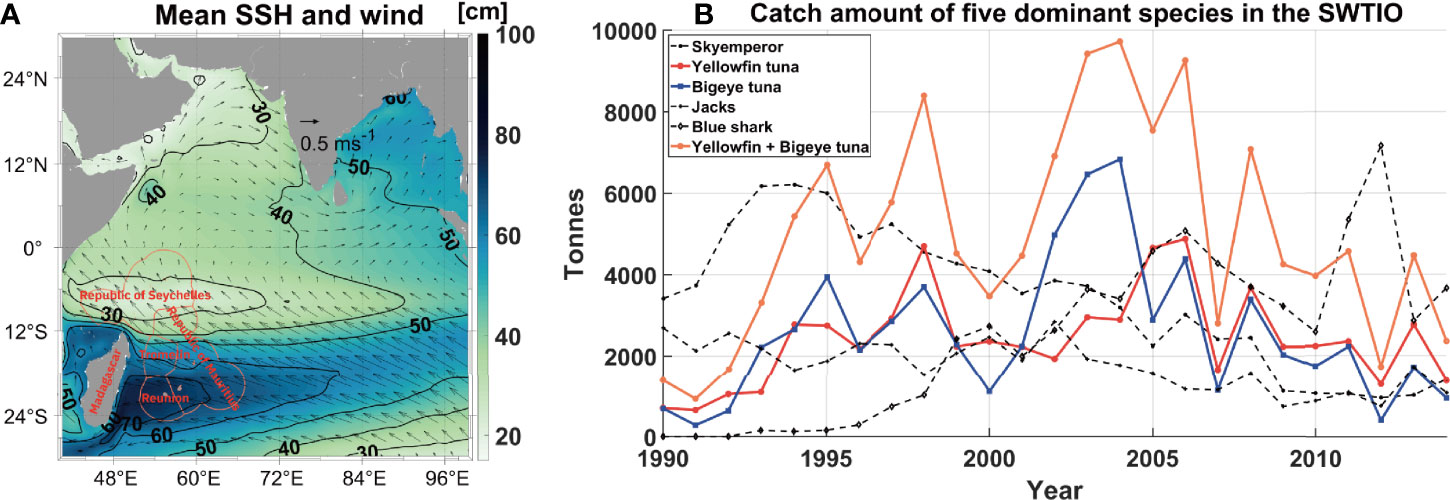
Figure 1 (A) Mean sea surface height (SSH) (color shading and contours) and wind velocity (vectors) in the tropical Indian Ocean for 1990–2014. Red contour lines illustrate the boundaries of the four exclusive economic zones (the Republic of Seychelles, the Republic of Mauritius, Tromelin Island, and Reunion Island) in the southwestern tropical Indian Ocean (SWTIO). (B) The annual catch amounts of the five dominant species (skyemperor, yellowfin tuna, bigeye tuna, jacks, and blue shark) in the SWTIO during 1990–2014. The red and blue lines denote the catch amounts of yellowfin tuna and bigeye tuna, respectively, and the orange line denotes the catch amount of Thunnus genus (yellowfin tuna + bigeye tuna).

The YFT inhabits the sea surface to the thermocline depth, possibly because they prefer relatively warm water (Kumari et al., 1993; Song et al., 2008; Houssard et al., 2017) or it is easier to access rich food sources in the surface layer (Kumari et al., 1993; Lehodey, 2004; Matsumoto et al., 2016; Houssard et al., 2017). The BET, however, inhabits the sea surface to the deeper ocean (but shallower than approximately 500 m) with relatively cold water (17–22°C) (Holland et al., 1992; Hampton et al., 1998; Holland and Grubbs, 2007; Song et al., 2009). The BET tends to be more tolerant of the environment with low oxygen, compared to other tropical tuna species (Holland et al., 1992; Lowe et al., 2000; Dagorn et al., 2000; Brill et al., 2005).

The adult YFT is generally caught by purse seine and longline fisheries (IOTC, 2009). The majority of adult BET is captured by longline fleets, but some are caught by purse seine in the subtropical region (Hampton et al., 1998; Fonteneau and Pallares, 2005; Holland and Grubbs, 2007). Lan et al. (2013) reported that the YFT catch amount tends to increase as the thermocline depth becomes shallower, which was associated with upwelling-induced enhancement of biological productivity in the northern and western margins of the western Indian Ocean. Additionally, the BET catch was reported to increase when the 20°C isotherm depth (D20) becomes shallower in the North Atlantic (Lan et al., 2018).

The El Niño–Southern Oscillation (ENSO) is closely associated with the distribution of pelagic tuna in the Pacific Ocean (Lehodey et al., 1997; Lehodey, 2004; Kim et al., 2020). Previous studies reported that the ENSO-related ocean environmental variability, particularly the upwelling variability, affects the catch amounts of pelagic tuna (Lehodey et al., 1997). In the Indian Ocean, the Indian Ocean Dipole (IOD) is known to influence the upwelling conditions (Saji et al., 1999). During the negative phase of the IOD, the increase of the YFT catch in the western Indian Ocean (including the marginal and high seas) has been reported to be associated with a shoaling of near-surface isotherms and an increase in primary production and food availability (Kumari et al., 1993; Mohri and Nishida, 2000; Ménard et al., 2007; Lan et al., 2013).

The isotherm depths exhibit a meridional difference between the northern (0°–12°S, EEZ of the Republic of Seychelles) and southern SWTIO (12°S–25°S, EEZs of the Republic of Mauritius, Tromelin Island, and Reunion Island). The mean sea surface height (SSH) is relatively low in the northern region compared to that in the southern region (Figure 1A). This meridional difference in SSH is mainly due to a prominent upwelling in the northern SWTIO, which is called the Seychelles–Chagos Thermocline Ridge (SCTR, 5°–10°S) (Hermes and Reason, 2008; Vialard et al., 2009). Hence, isotherms, including the thermocline and D20, are shallower in the northern region. Changes in the isotherm depths and the associated upwelling variability could play a major role in the interannual variability of the YFT and BET catches in SWTIO.

The upwelling conditions develop due to both local wind forcing and remote forcing via westward propagation of upwelling Rossby waves, which tend to occur during the negative phase of the IOD and the ENSO years (Marsac and Le Blanc, 1999; Lehodey et al., 2006; Ménard et al., 2007; Lan et al., 2013; Lan et al., 2020). However, due to the meridional differences in the ocean environment, upwelling conditions would develop differently throughout the SWTIO. Accordingly, the relationship between the YFT catch amount and the thermocline depth previously reported in the Indian Ocean (Lan et al., 2013), could be different in the northern and southern regions of the SWTIO.

This study aimed to investigate the meridional differences in the relationships between the YFT and the BET catches and the ocean environmental variability in the SWTIO by analyzing the interannual variability of the catch amount during 1990–2014 (25 years). To understand the local and remote influences on the upper-ocean (< 400 m) variability, temperature, salinity, and ocean currents were examined in the wider tropical Indian Ocean. This comprehensive analysis of the various ocean environmental variables, beyond temperature variability, will clarify the link between the catch amounts in the SWTIO and climate variability, including the IOD and ENSO.

Materials and Methods

Fisheries Data

This study investigated the temporal variability of YFT and BET catch amounts in the northern region (the Republic of Seychelles) and the southern region (the Republic of Mauritius + Tromelin Island + Reunion Island) of the SWTIO (Figure 1A). The annual catch amounts of the four EEZs were obtained from Sea Around Us (SAU, http://www.seaaroundus.org) for 1990–2014 (Boistol et al., 2011; Le Manach et al., 2015a; Le Manach et al., 2015b; Le Manach and Pauly, 2015). The catch data were based on officially reported data from the Food and Agriculture Organization of the United Nations (http://www.fao.org/fishery/statistics/en), but were improved by including unreported catches and major discards (Pauly and Zeller, 2015; Pauly and Zeller, 2016). However, the unreported catch amounts of YFT and BET are more than one order smaller than the reported catch amounts in the four EEZs. For example, the unreported YFT catch amount in the Republic of Seychelles is about 15 tonnes on average during 1990–2014.

Ocean Environmental Variables

The monthly sea surface height and upper 400 m temperature, salinity, and current velocity were obtained from the Simple Ocean Data Assimilation (SODA) 3.4.2, with a spatial resolution of 0.5° × 0.5° for 1988–2016 (Carton et al., 2018). The relationship between the tuna catches and the ocean environment was analyzed for the overlapping period, that is, 1990–2014, and the extra years, i.e., 1998–1999 and 2015–2016, were used to examine the lead-lag relationship with the climate indices. The thermocline depth and D20 were calculated from the SODA 3.4.2 data at each grid point, after conducting vertical linear interpolation of the temperature every 1 m. Monthly mean 10 m wind velocity and total precipitation were obtained for the same period (1988–2016) with a horizontal resolution of 0.25° × 0.25° from ERA5, which is the fifth generation atmospheric reanalysis from the European Centre for Medium Range Weather Forecasts. The ERA5 is based on 4D-Var data assimilation using global observation data (Hersbach et al., 2020). Monthly mean net primary production and chlorophyll concentration in the upper 400 m of the ocean were obtained for 1993–2016 with a resolution of 0.25° × 0.25°V from the Global Ocean Biogeochemistry Hindcast from Mercator-Ocean, provided by the Copernicus Marine Environment Monitoring System Service. This biogeochemical hindcast is based on the PISCES biogeochemical model, available on the Nucleus for European Modelling of the Ocean modelling platform (Perruche et al., 2019).

Cyclostationary Empirical Orthogonal Function (CSEOF) Analysis

The CSEOF analysis (Kim et al., 1996; Kim and North, 1997) was used to extract the spatio-temporal variability of the environmental variables in the wider tropical Indian Ocean (30°N to 30°S and 40°E to 100°E, Figure 1A), including sea surface height, temperature, salinity, current velocity, 10 m wind velocity, total precipitation, net primary production, and chlorophyll concentration. The CSEOF technique has been applied by various studies to understand the relationship between a specific time series and the spatio-temporal variability of geophysical variables (Kim et al., 2015), including a study on the relationship between tuna fisheries and ocean environmental variability in the western equatorial Pacific (Kim et al., 2020).

In CSEOF, the environmental variables at each depth, A(r, t), were decomposed as cyclostationary loading vectors (CSLVs), B_n(r, t)VV and their corresponding principal component (PC) time series, C_n(t) as in Eq. (1):

$\begin{array}{ll}A(r,t)={\Sigma }_n{B}_n\left(r,t\right)C_n\left(t\right),& (1)\end{array}$

where n, r, and t denote the mode number, 2-dimensional space, and time, respectively. Note that the CSEOF analysis was separately conducted on each environmental variable at each depth. For example, a total of 22 CSEOF decomposition was carried out for temperature, as the SODA provides 22 vertical levels in the upper 400 m. CSLVs illustrate the physical evolution of environmental variables with a nested period d, which was set to 12 months in this study. The nth mode of the CSLVs is expressed with periodicity d, as in Eq. (2):

$\begin{array}{ll}{B}_n(r,t)=B_n(r,t+d).& (2)\end{array}$

The corresponding PC time series, C_n(t), illustrates the temporal variation of B_n(r, t) for 1988–2016, except for net primary production and chlorophyll concentration, which are available for 1993–2016.

Regression Analysis

A regression analysis was applied for each environmental variable at each depth, targeting the annual fishery time series, F(t) of the northern and southern regions separately, as shown in Eq. (3):

$\begin{array}{ll}F\left(t\right)\approx {\sum }_{m=1}^{10}{\alpha }_m{\tilde{C}}_m(t),& (3)\end{array}$

where m denotes the mode number, α_m is the regression coefficient, and is the annually averaged mth mode of the PC time series extracted from the environmental variables (predictor variables). The regression was conducted for the period of the target fishery data, 1990–2014 (1993–2014 for net primary production and chlorophyll), using the annual mean of C_m(t), because the target time series, F(t), are only available as the annual mean catch amounts. Note that the predictor PC time series, C_m(t), are uncorrelated to each other for each regression.

The regressed and reconstructed CSLVs, R(r,t), that illustrate the environmental variability related to the annual catch amounts, are obtained by using the regression coefficients, α_m as in Eq. (4):

$\begin{array}{ll}R\left(r,t\right)={\sum }_{m=1}^{10}{\alpha }_m{B}_m\left(r,t\right),& (4)\end{array}$

where each R(r, t) consists of 12 monthly spatial patterns of each variable at each depth, same as B_m(r, t). Thus, the R(r, t) exhibits consistent temporal variability with the target time series F(t) with the error in Eq. (3). The number of PC time series used in the regression was set to ten in order to avoid a possible overfitting or underfitting issue. The R-squared values of the regression are shown in Supplementary Figure 1, and those of net primary production and chlorophyll concentration are shown in Supplementary Figure 2. If the R-squared value is relatively low for a specific variable at a specific depth, it indicates that the ocean environmental variability at the depth is not closely related to the target variability, i.e., the annual catch amount of YFT or BET in the northern or southern regions of the SWTIO. The annually averaged spatial patterns of each R(r, t)are presented in this study, focusing on the interannual variability.

The relationship between the ocean environmental variability and the IOD and ENSO was investigated using the same regression analysis, but using the monthly PC time series of the environmental variables, as the Indian Ocean Dipole Mode Index (DMI) and the Multivariate ENSO Index (MEI) are available as monthly means (Saji et al., 1999; Zhang et al., 2019). The regression analysis was also conducted by employing time lags between the ocean environmental variables and climate indices because the IOD and ENSO exhibit low-frequency variabilities that last longer than a year. A series of lagged regression analyses were conducted with time lags of ± 1 year (e.g., 1989–2013 and 1991–2015) and ±2 years (e.g., 1988–2012 and 1992–2016), targeting the DMI and MEI. The R-squared values of the lagged regression analysis are shown in Supplementary Figure 5. The R-squared values of the regression are shown at each depth in Supplementary Figure 3.

Results

Ocean Environment and Tuna Catches in the SWTIO

Figure 2 illustrates the zonally averaged mean and standard deviation of the temperature, salinity, and zonal and meridional current velocity in the upper 400 m of the SWTIO. The mean thermocline depth is shallower in the northern region (northern: ~66 m, southern: ~87 m), which is associated with the SCTR, and the peak of the SCTR (shallowest thermocline depth) is observed at approximately 8°S (Figure 2A). The mean D20 is shallower (~91 m) and closer to the thermocline depth in the northern region, but the mean D20 is substantially deeper (~163 m) in the southern region. In the northern region, the near-surface (< D20) is more saline, but the deeper layer (> D20) is more saline in the southern region (Figure 2B). The fresh near-surface water in the southern region is from the Indonesian Throughflow in the equatorial eastern Indian Ocean (Gordon et al., 1997; Makarim et al., 2019). The mean zonal currents show meridionally opposing directions, reflecting the southeastward-flowing South Equatorial Counter Current (SECC) to the north of the SCTR (north of approximately 8°S) and the southwestward-flowing South Equatorial Current (SEC) to the south of the SCTR (Figures 2C, D).

FIGURE 2

Figure 2 Meridional distribution of the (top) means and (bottom) standard deviations of the ocean environmental variables for 1990–2014, zonally averaged from 54°E to 60°E in the SWTIO. The standard deviations were calculated from the annual means of the variables. Each column represents a different variable: (A) temperature, (B) salinity, (C) zonal current velocity, and (D) meridional current velocity. The thick dashed/dotted lines and solid lines indicate the mean thermocline depth and 20°C isotherm depth (D20), respectively. The vertical dashed lines denote 12°S, the boundary between the northern and southern regions of the SWTIO.

The temporal variations in the environmental variables also exhibit meridional differences on the interannual time scale (see the bottom of Figure 2). Due to the strong subsurface upwelling variability in the SCTR, the standard deviation of the upper ocean (< 400 m) temperature is larger near the thermocline depth and D20 in the northern region. In both regions, salinity exhibits significant variability from the surface to the thermocline depth, which is deeper in the southern region. The standard deviations of the zonal and meridional currents are larger in the northern region, where the SECC flows southeastward. The different ocean environmental conditions in the northern and southern regions shown in Figure 2 may contribute to the YFT and BET catch variability in the SWTIO.

Figure 3 displays the annual catch amount of the YFT and the BET in the SWTIO for 1990–2014. The YFT and BET catch amounts throughout the SWTIO exhibit similar variability, except for a few years in the early 2000s (Figure 3A). This similarity between the YFT and BET catch amounts is also observed separately in the northern and southern regions (Figures 3B, C). In the northern region, both YFT and BET catches were larger in the 1990s and the early 2000s, compared to the late 2000s and early 2010s. In the southern region, however, the catches were smaller in the 1990s than in later years. The difference between the YFT and BET catch variability seems not to be significant as the difference of the catch variability between the northern and southern regions.

FIGURE 3

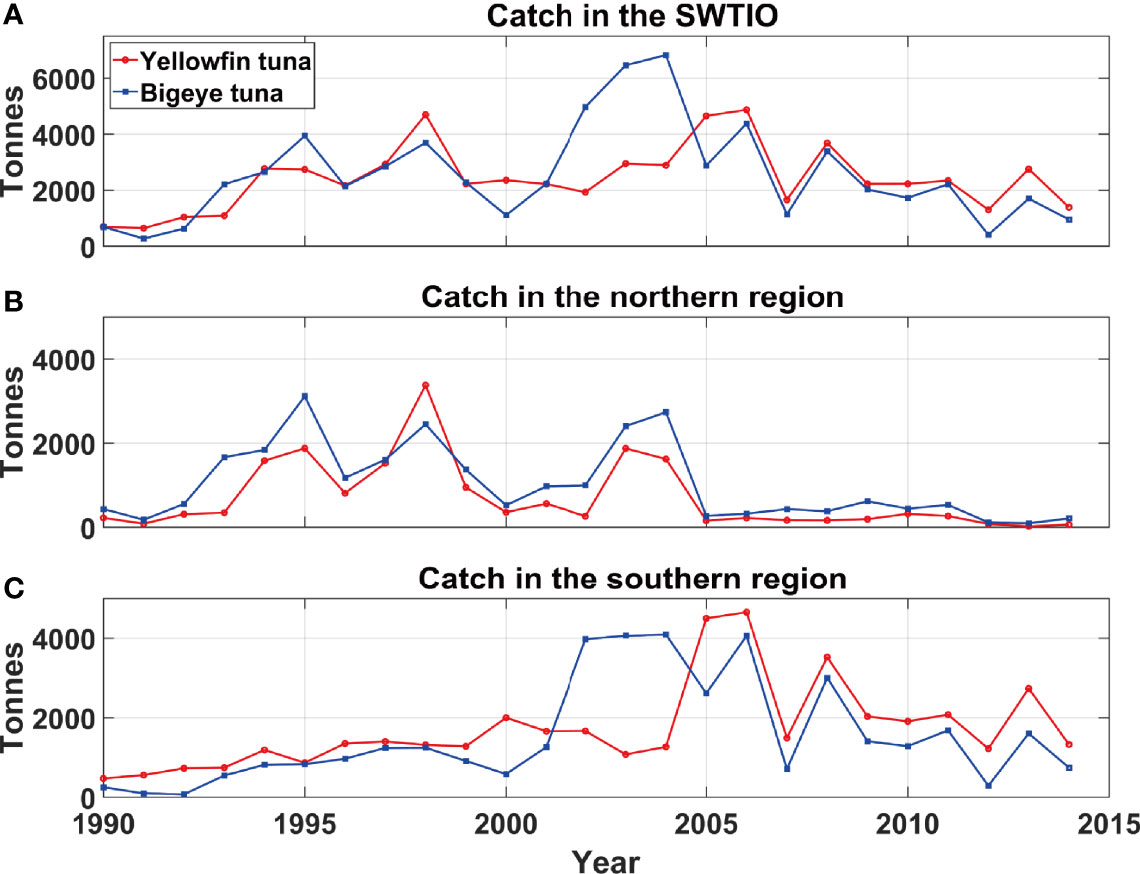
Figure 3 (A) The annual catch amounts of yellowfin tuna and bigeye tuna during 1990–2014 in the four exclusive economic zones (EEZs) of the entire SWTIO. (B) The same as (A), but only for the northern region of the SWTIO (the Republic of Seychelles). (C) The same as (B), but only for the southern region of the SWTIO (the Republic of Mauritius, Tromelin Island, and Reunion Island).

Ocean Conditions During the Catch Increase

Figure 4 illustrates the regressed anomalies of the ocean conditions during the increase of the YFT and the BET in the northern and southern regions of the SWTIO. The R-squared values of the regression for each variable and each depth are presented in Supplementary Figure 1. The temperature conditions, during the increase of the YFT and the BET catches in the northern region, represent strong positive anomalies near the mean thermocline depth and D20 in the northern region (top two rows in Figure 4A). They also exhibit the negative anomalies below the thermocline depth and D20 in the northern SCTR. The temperature anomalies indicate the deeper isotherms in the southern SCTR and the shallower isotherms in the northern SCTR, thus the flattening of the isotherms in the SCTR, during the increase of the catch in the northern region. The flattening of the isotherms suggests the suppression of the subsurface upwelling in the SCTR. On the contrary, the temperature conditions, during the increase of the YFT and the BET catches in the southern region, represent relatively weak positive anomalies in the southern region (bottom two rows in Figure 4A).

FIGURE 4

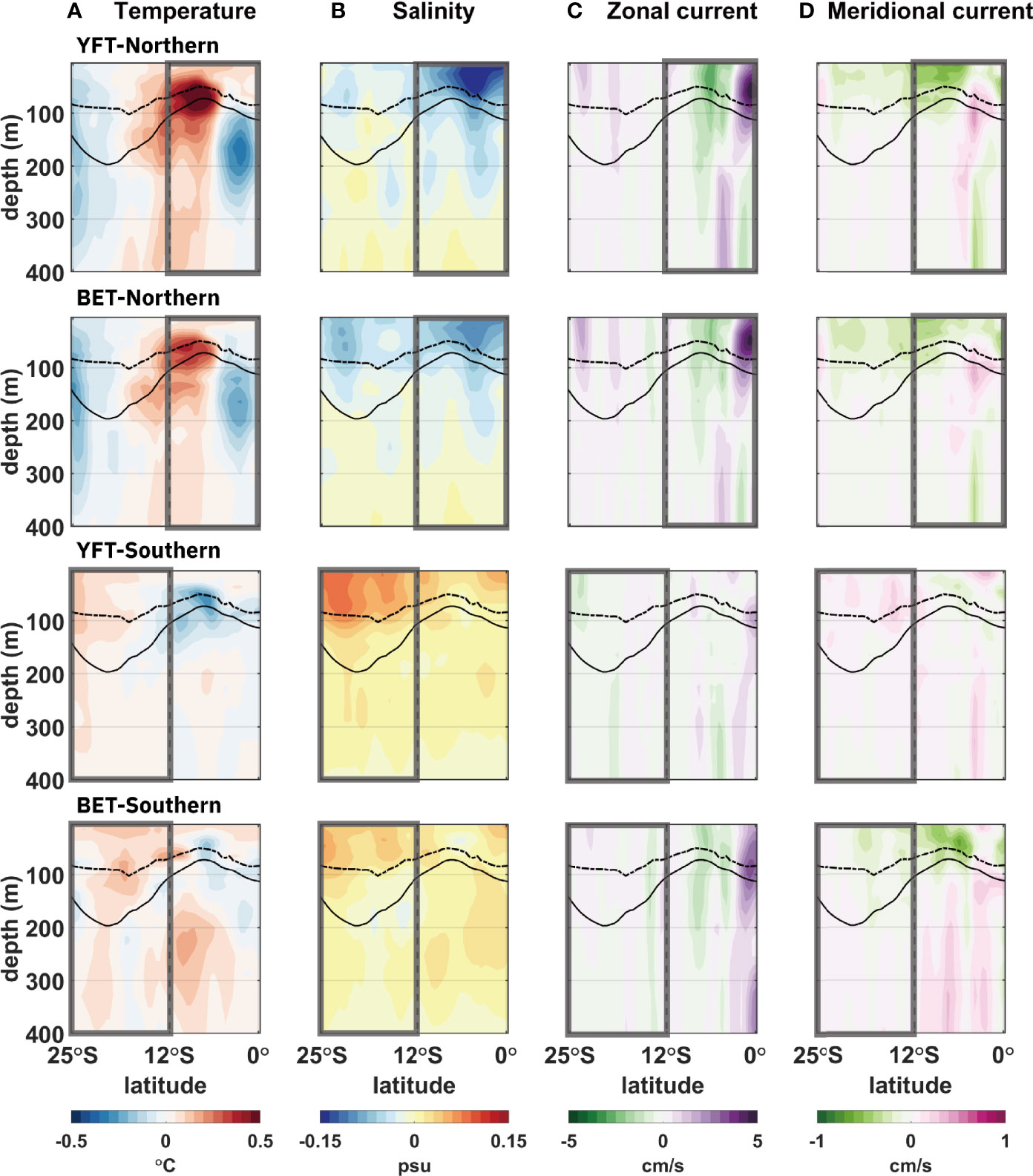
Figure 4 Meridional distributions of the regressed and reconstructed anomalies of the ocean environmental variables during 1990–2014. Target time series are the annual catch amounts of yellowfin tuna (YFT) and bigeye tuna (BET) in the northern (top two rows) and southern (bottom two rows) regions; the target time series are referred as YFT-Northern, BET-Northern, YFT-Southern, and BET-Southern, respectively. The anomalies are presented after zonal averages from 54°E to 60°E. Each column represents a different variable: (A) temperature (shading intervals: 0.05°C), (B) salinity (shading intervals: 0.015 psu), (C) zonal current velocity (shading intervals: 0.5 cm/s), and (D) meridional current velocity (shading intervals: 0.1 cm/s). The thick dashed/dotted lines and solid lines indicate the mean thermocline depth and D20, respectively. The gray boxes indicate the northern or southern region of the SWTIO, denoting the region of each target time series.

The salinity conditions, during the increase of the YFT and the BET catches in the northern region, exhibit similar anomalies with the near-surface (< D20) freshening in the northern region (top two rows in Figure 4B). Those freshening in the northern region is consistent with an increase of precipitation in this region (top row in Supplementary Figure 4). On the other hand, the positive salinity anomalies and the decrease of precipitation are detected in the southern region during the increase of the YFT and the BET catches in the southern region (bottom two rows in Figure 4B and middle row in Supplementary Figure 4). The negative anomalies in the north and the positive anomalies in the south contribute to the similar near-surface salinity ranges of 34.8–35.2 psu, which is within the favorable salinity range for an increase of the YFT and the BET catches reported in the Indian Ocean (Song et al., 2008; Song et al., 2009).

The current velocity conditions in the northern region during the increase of the YFT and the BET catches in the northern region exhibit larger anomalies of zonal current velocity compared to those of meridional current velocity (close to an order of magnitude of difference) (top two rows in Figures 4C, D). They exhibit westward anomalies at the latitude near the SCTR upwelling peak and the eastward anomalies to the north of the peak. It indicates the equatorward shift of the SEC in comparison with the mean current velocity in Figures 2C, D. The equatorward shift is consistent with the easterly wind anomalies near the equator during the increase of YFT and BET catches in the northern region (top row in Supplementary Figure 4). The regressed anomalies of current velocity targeting the YFT and the BET catches in the southern region are relatively smaller (bottom two rows in Figures 4C, D), similar to the results of the temperature regression.

Ocean Conditions During the Positive Phase of the IOD and the ENSO

Figure 5 illustrates the ocean environmental conditions in the SWTIO during the positive phase of the IOD and the ENSO. The R-squared values of the regressions are displayed in Supplementary Figure 3. The strong positive temperature anomalies are observed near the thermocline depth and D20 in the northern region during the positive phase of both the IOD and the ENSO, indicating the suppression of SCTR upwelling (Figure 5A). The current velocity conditions represent an equatorward shift in the SEC during the positive phase of both the IOD and the ENSO (Figures 5C, D).

FIGURE 5

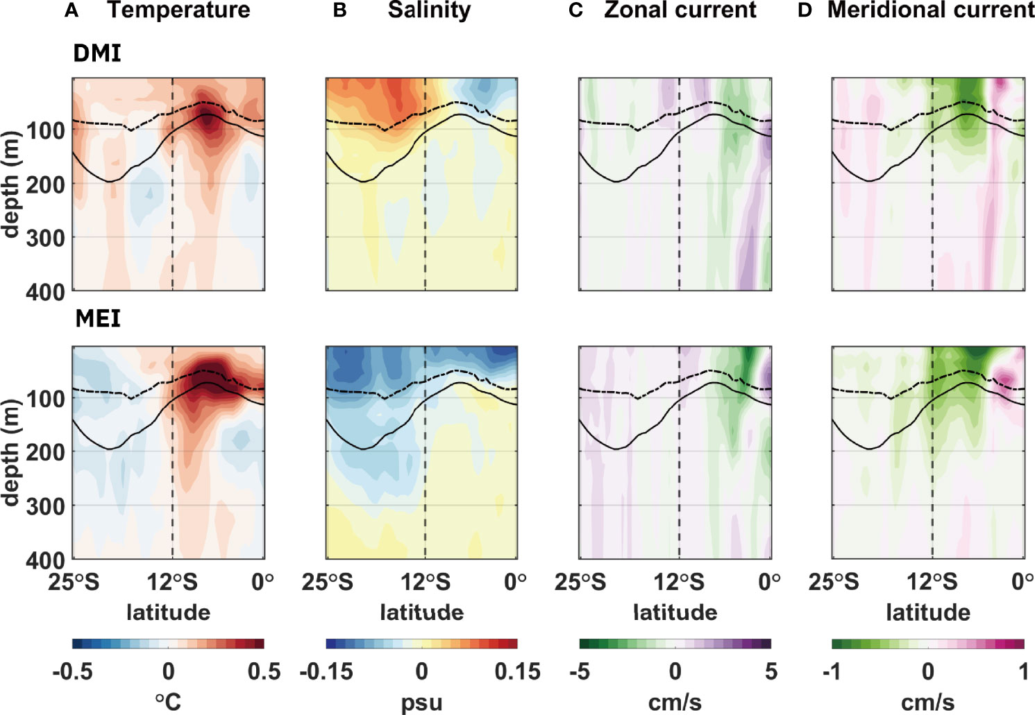
Figure 5 Meridional distribution of the regressed and reconstructed anomalies of the ocean environmental variables with respect to the normalized Indian Ocean dipole mode index (DMI; top) and normalized multivariate El Niño–Southern Oscillation (ENSO) index (MEI; bottom) for 1990–2014. The anomalies are presented after zonal averages from 54°E to 60°E. Each column represents a different variable: (A) temperature (shading intervals: 0.05°C), (B) salinity (shading intervals: 0.015 psu), (C) zonal current velocity (shading intervals: 0.5 cm/s), and (D) meridional current velocity (shading intervals: 0.1 cm/s). The thick dashed/dotted lines and solid lines indicate the mean thermocline depth and D20, respectively. The vertical dashed lines denote 12°S, the boundary between the northern and southern regions of the SWTIO.

However, the salinity conditions are different between the positive phase of the IOD and the ENSO (Figure 5B). During the positive phase of the IOD, the salinity anomalies exhibit different signs between the northern and southern regions (top of Figure 5B). The dipole-like pattern of salinity anomaly was previously reported as a Salinity-IOD Mode that originated from the eastern tropical Indian Ocean (Zhang et al., 2016). On the other hand, during the positive phase of the ENSO, the salinity condition reflects an overall near-surface freshening in both northern and southern regions (bottom of Figure 5B). The regression of the precipitation generally exhibits consistent patterns with the regressed salinity anomalies (Supplementary Figure 4).

Discussion

The temporal variability of the temperature and current velocity is smaller in the southern region, compared to those in the northern region (bottom of Figure 2). Moreover, the regressed anomalies of temperature and current velocity are relatively weak when targeting the catches in the southern region. It suggests that it would be difficult to investigate the catch favorable ocean conditions in the southern region. Also, the R-squared values are smaller when targeting the catches in the southern region, compared to those targeting the northern region. It implies that the catch favorable ocean conditions can be difficult to be explored for the region where the natural variability is weak.

However, it is clearly shown that the SCTR upwelling suppresses during the increase of the catch in the northern region, where the background natural variability is strong. Previous studies have suggested that upwelling-induced shallower isotherms are associated with an increase of YFT and BET catches in the western Indian Ocean (Marsac and Le Blanc, 1999; Lehodey et al., 2006; Ménard et al., 2007; Lan et al., 2020). This seems reasonable because upwelling generally increases near-surface productivity, which would be favorable for pelagic tuna (Hermes and Reason, 2008; Vialard et al., 2009). However, the regression results exhibit a meridional flattening of the isotherms, which indicates the suppression of the SCTR upwelling (top two rows in Figure 4). This discrepancy may be explained by the distinct ocean environment of the subsurface upwelling in the northern SWTIO.

Figure 6 shows the mean and regressed anomalies of the net primary production and chlorophyll concentration targeting the tuna catches in the SWTIO for 1993–2014 (22 years). The R-squared values of the regression for each depth are presented in Supplementary Figure 2. In the northern region, the mean net primary production is higher in the near-surface layer, and the mean chlorophyll concentration shows a maximum near the D20 and thermocline depth. The regressed anomalies, targeting the catch variability in the northern SWTIO, exhibit both positive and negative anomalies at different depths and latitudes. However, the depth-integrated anomalies are generally positive to the north of the peak of the SCTR, but negative to the south, which contributes to the area-averaged anomalies becoming close to zero. This indicates that there is no significant increase in the biological activity when the YFT and BET catch increase. A plausible hypothesis would be that, in the northern SWTIO where the mean biological activity is high, the upwelling suppression may vertically extend the favorable habitat of the pelagic tuna, even without an increase in biological activity. The deepening of isotherms itself could contribute to an extension of the fishing ground and thus increase the YFT and BET catches.

FIGURE 6

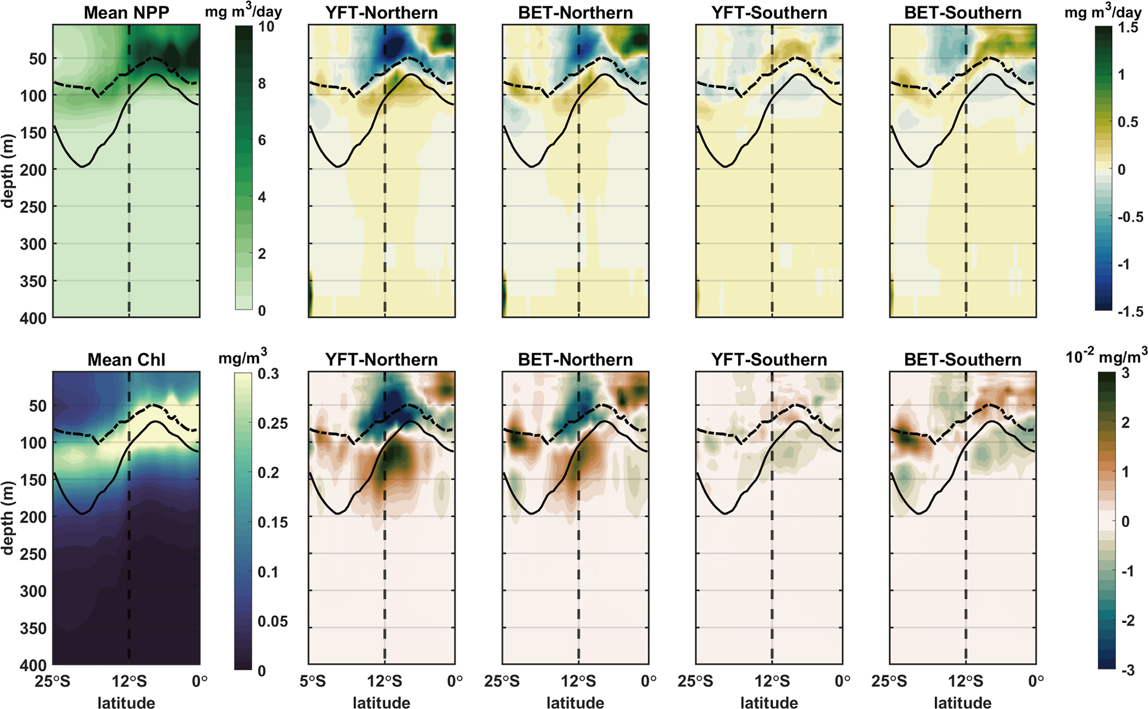
Figure 6 Meridional distribution of the mean (first column) and the regressed and reconstructed anomalies of the net primary production (NPP; upper row) and chlorophyll concentration (Chl; lower row) during 1993–2014. Target time series are the annual catch amounts of yellowfin tuna (YFT) and bigeye tuna (BET) in the northern (second and third columns) and southern (fourth and last columns) regions of the SWTIO. The anomalies are presented after zonal average from 54°E to 60°E. The thick dashed/dotted lines and solid lines indicate the mean thermocline depth and D20, respectively.

The overall temperature and current velocity conditions during the positive phase of the IOD and the ENSO are similar to those during the increase of the YFT and the BET catches in the northern region (top two rows in Figures 4 and 5). The SCTR upwelling suppression and equatorward shift of the SEC seem to occur during the positive phase of both the IOD and ENSO. Despite the similarities, the salinity condition during the positive phase of the IOD is significantly different (top of Figure 5B). It indicates that the ocean environmental conditions during the increase of the catch in the northern region are similar to those during the El Niño years (positive phase of the ENSO), rather than those during the positive phase of the IOD. The direct correlation coefficients between the MEI and the YFT and the BET catches in the northern region are 0.29 and 0.30, respectively, while those between the DMI and the YFT and the BET catches in the northern region are 0.18 and 0.06, respectively. The correlation coefficients between the climate indices and the catches in the southern region are all insignificant.

The lagged-regression results between the catch variability and climate indices also suggest a possible closer relationship to the ENSO, rather than to the IOD (Supplementary Figures 6, 7). The distinct temperature anomalies from the zero-lag regression in Figure 5 develop in the northern region during El Niño years and continue throughout the following years, while the temperature anomalies almost disappear one year after the positive IOD years. The direct correlation coefficients between the MEI and the YFT and the BET catches in the northern region are 0.53 and 0.52, respectively, when applying the one-year lag. Those of the DMI are all insignificant, which may support the closer relationship between the ENSO and the catch variability in the northern region.

Finally, this study used the annual catch amount as the target time series, not normalized by catch effort, because the catch per unit effort is not publicly available for the study region. Considering this limitation, this study limited the analysis period after the 1990s, assuming that the possible changes in catch effort and fishing methods do not significantly influence the relationship between the catch and ocean environmental variability for the recent decades (1990–2014). The temporal changes in the catch effort and fishing methods may be considered as “anthropogenic” factors and become a source of regression error in finding a relationship with the “natural” ocean environmental variability. The reliable usage of the catch data for specific EEZs in recent decades, on behalf of the catch per unit effort data, was also shown for skipjack tuna in the western tropical Pacific (Kim et al., 2020).

Conclusion

This study presented the ocean environmental conditions during the increase of the YFT and BET catches in the SWTIO on the interannual time scale. The catch-favorable ocean environment is distinct only in the northern region, where the subsurface upwelling variability is prominent over the SCTR. The meridional flattening of the isotherms, resulting in the subsurface upwelling suppression, is associated with the increase of both the YFT and the BET catches in the northern region. This contradicts previous studies in the western Indian Ocean, which suggested an increase in upper-ocean productivity in fisheries during upwelling, indicating a complex relationship between the ocean environmental variability and the catch variability. The ocean environmental conditions, linked to the increase of the YFT and the BET catches in the northern region, seem to develop during El Niño years and last through the following year. The significant relationship between the catch amount and the ENSO with a one-year lag suggests possible predictability of the YFT and the BET catch amounts for the sustainable fishery in the SWTIO.

Data Availability Statement

The original contributions presented in the study are included in the article/Supplementary Material. Further inquiries can be directed to the corresponding author.

Author Contributions

JK conducted the analysis and prepared the figures. JK and HN designed the research, discussed the results, and wrote the manuscript. All authors contributed to the article and approved the submitted version.

Funding

This work was supported by the National Research Foundation of Korea (NRF) grant funded by the Korea government (MSIT) (No. 2019R1C1C1010446) and the Ministry of Oceans and Fisheries, Republic of Korea through the joint application program of research vessel in 2019 (PE99794).

Conflict of Interest

The authors declare that the research was conducted in the absence of any commercial or financial relationships that could be construed as a potential conflict of interest.

Publisher’s Note

All claims expressed in this article are solely those of the authors and do not necessarily represent those of their affiliated organizations, or those of the publisher, the editors and the reviewers. Any product that may be evaluated in this article, or claim that may be made by its manufacturer, is not guaranteed or endorsed by the publisher.

Supplementary Material

The Supplementary Material for this article can be found online at: https://www.frontiersin.org/articles/10.3389/fmars.2022.857405/full#supplementary-material

References

Boistol L., Harper S., Booth S., Zeller D. (2011). Reconstruction of Marine Fisheries Catches for Mauritius and Its Outer Islands, 1950-2008. pp. 39-61. In: Harper S., Zeller D. (eds.) Fisheries Catch Reconstructions: Islands, Part II. Fisheries Centre Research Reports (Fisheries Centre: University of British Columbia) 19 (4), 39.

Google Scholar

Brill R. W., Bigelow K. A., Musyl M. K., Fritsches K. A., Warrant E. J. (2005). Bigeye Tuna (Thunnus Obesus) Behavior and Physiology and Their Relevance to Stock Assessments and Fishery Biology. Col. Vol. Sci. Pap. ICCAT. 57 (2), 142–161.

Google Scholar

Carton J. A., Chepurin G. A., Chen L. (2018). SODA3: A New Ocean Climate Reanalysis. J. Clim. 31 (17), 6967–6983. doi: 10.1175/JCLI-D-18-0149.1

CrossRef Full Text | Google Scholar

Dagorn L., Bach P., Josse E. (2000). Movement Patterns of Large Bigeye Tuna (Thunnus Obesus) in the Open Ocean, Determined Using Ultrasonic Telemetry. Mar. Biol. 136 (2), 361–371. doi: 10.1007/s002270050694

CrossRef Full Text | Google Scholar

Fonteneau A., Pallares P. (2005). Tuna Natural Mortality as a Function of Their Age: The Bigeye Tuna (Thunnus Obesus) Case. ICCAT. Col. Vol. Sci. Pap. 57, 127–141.

Google Scholar

Gordon A. L., Ma S., Olson D. B., Hacker P., Ffield A., Talley L. D., et al. (1997). Advection and Diffusion of Indonesian Throughflow Water Within the Indian Ocean South Equatorial Current. Geophys. Res. Lett. 24 (21), 2573–2576. doi: 10.1029/97GL01061

CrossRef Full Text | Google Scholar

Hampton J., Bigelow K., Labelle M. (1998). Effect of Longline Fishing Depth, Water Temperature and Dissolved Oxygen on Bigeye Tuna (Thunnus Obesus) Abundance Indices. Ocean. Fisheries. Programme. Secretariat. Pacific. Community. New Caledonia. 18.

Google Scholar

Hermes J. C., Reason C. J. C. (2008). Annual Cycle of the South Indian Ocean (Seychelles-Chagos) Thermocline Ridge in a Regional Ocean Model. J. Geophys. Res. Ocean. 113 (C4), C04035. doi: 10.1029/2007JC004363

CrossRef Full Text | Google Scholar

Hersbach H., Bell B., Berrisford P., Hirahara S., Horányi A., Muñoz-Sabater J., et al. (2020). The ERA5 Global Reanalysis. Q. J. R. Meteorol. Soc. 146 (730), 1999–2049. doi: 10.1002/qj.3803

CrossRef Full Text | Google Scholar

Holland K. N., Brill R. W., Chang R. K., Sibert J. R., Fournier D. A. (1992). Physiological and Behavioural Thermoregulation in Bigeye Tuna (Thunnus Obesus). Nature 358 (6385), 410–412. doi: 10.1038/358410a0

PubMed Abstract | CrossRef Full Text | Google Scholar

Holland K. N., Grubbs R. D. (2007). “Fish Visitors to Seamounts: Tunas and Billfish at Seamounts”, in Seamounts: Ecology, Conservation and Management. Fish and Aquatic Resources Series, Ed. Tony J. P. (Oxford: Blackwell Scientific), 189–201.

Google Scholar

Houssard P., Lorrain A., Tremblay-Boyer L., Allain V., Graham B. S., Menkes C. E., et al. (2017). Trophic Position Increases With Thermocline Depth in Yellowfin and Bigeye Tuna Across the Western and Central Pacific Ocean. Prog. Oceanogr. 154, 49–63. doi: 10.1016/j.pocean.2017.04.008

CrossRef Full Text | Google Scholar

IOTC (2009). Report of the Twelfth Session of the Scientific Committee of the Indian Ocean Tuna Commsion Vol. 190 (Victoria: Seychelles).

Google Scholar

Kim K.-Y., Hamlington B., Na H. (2015). Theoretical Foundation of Cyclostationary EOF Analysis for Geophysical and Climatic Variables: Concepts and Examples. Earth-Sci. Rev. 150, 201–218. doi: 10.1016/j.earscirev.2015.06.003

CrossRef Full Text | Google Scholar

Kim J., Na H., Park Y.-G., Kim Y. H. (2020). Potential Predictability of Skipjack Tuna (Katsuwonus Pelamis) Catches in the Western Central Pacific. Sci. Rep. 10 (1), 1–8. doi: 10.1038/s41598-020-59947-8

PubMed Abstract | CrossRef Full Text | Google Scholar

Kim K.-Y., North G. R. (1997). EOFs of Harmonizable Cyclostationary Processes. J. Atmos. Sci. 54 (19), 2416–2427. doi: 10.1175/15200469(1997)054<2416:EOHCP>2.0.CO;2

CrossRef Full Text | Google Scholar

Kim K.-Y., North G. R., Huang J. (1996). EOFs of One-Dimensional Cyclostationary Time Series: Computations, Examples, and Stochastic Modeling. J. Atmos. Sci. 53 (7), 1007–1017. doi: 10.1175/15200469(1996)053<1007:EOODCT>2.0.CO;2

CrossRef Full Text | Google Scholar

Kumari B., Raman M., Narain A., Sivaprakasam T. (1993). Location of Tuna Resources in Indian Waters Using NOAA AVHRR Data. Int. J. Remote Sens. 14 (17), 3305–3309. doi: 10.1080/01431169308904446

CrossRef Full Text | Google Scholar

Lan K.-W., Chang Y.-J., Wu Y.-L. (2020). Influence of Oceanographic and Climatic Variability on the Catch Rate of Yellowfin Tuna (Thunnus Albacares) Cohorts in the Indian Ocean. Deep. Sea. Res. Part II 175, 104681. doi: 10.1016/j.dsr2.2019.104681

CrossRef Full Text | Google Scholar

Lan K.-W., Evans K., Lee M.-A. (2013). Effects of Climate Variability on the Distribution and Fishing Conditions of Yellowfin Tuna (Thunnus Albacares) in the Western Indian Ocean. Clim. Change 119 (1), 63–77. doi: 10.1007/s10584-012-0637-8

CrossRef Full Text | Google Scholar

Lan K.-W., Lee M. A., Chou C. P., Vayghan A. H. (2018). Association Between the Interannual Variation in the Oceanic Environment and Catch Rates of Bigeye Tuna (Thunnus Obesus) in the Atlantic Ocean. Fish. Oceanogr. 27 (5), 395–407. doi: 10.1111/fog.12259

CrossRef Full Text | Google Scholar

Lehodey P. (2004). “Climate and Fisheries: An Insight From the Pacific Ocean,” in Ecological Effects of Climate Variations in the North Atlantic - A Comparative Perspective. Eds. Stenseth N. C., Ottersen G., Hurrel J. (A. Belgrano: Oxford University press), 137–146.

Google Scholar

Lehodey P., Alheit J., Barange M., Baumgartner T., Beaugrand G., Drinkwater K., et al. (2006). Climate Variability, Fish, and Fisheries. J. Clim. 19 (20), 5009–5030. doi: 10.1175/JCLI3898.1

CrossRef Full Text | Google Scholar

Lehodey P., Bertignac M., Hampton J., Lewis A., Picaut J. (1997). El Niño Southern Oscillation and Tuna in the Western Pacific. Nature 389 (6652), 715–718. doi: 10.1038/39575

CrossRef Full Text | Google Scholar

Le Manacha F., Cisneros-Montemayorc A. M., Lindopa A., Padillaa A., Schillera L., Zellera D., et al. (2014). Global Catches of Large Pelagic Fishes, With Emphasis on Tuna in the High Seas Vol. 25 (Vancouver, B.C., Canada: Online Publication. Sea Around Us). Available at: www.seaaroundus.org.

Google Scholar

Le Manach F., Bach P., Barret L., Guyomard D., Fleury P. G., Sabarros P. S., et al. (2015a). “Reconstruction of the Domestic and Distant Water Fisheries Catch of La Réunion (France), 1950–2010,” in Fisheries Centre Research Reports, vol. 23. (Vancouver: The University of British Columbia), 83–98.

Google Scholar

Le Manach F., Bach P., Boistol L., Robinson J., Pauly D. (2015b). “Artisanal Fisheries in the World’s Second Largest Tuna Fishing Ground-Reconstruction of the Seychelles’ Marine Fisheries Catch 1950–2010,” in Fisheries Centre Research Reports, vol. 23. (Vancouver: The University of British Columbia), 99–110.

Google Scholar

Le Manach F., Pauly D. (2015). First Estimate of Unreported Catch in the French Îles Éparses 1950–2010. Fisheries Centre Research Reports Vol. 23 (Vancouver: The University of British Columbia), 27–35.

Google Scholar

Lowe T., Brill R., Cousins K. (2000). Blood Oxygen-Binding Characteristics of Bigeye Tuna (Thunnus Obesus), a High-Energy-Demand Teleost That is Tolerant of Low Ambient Oxygen. Mar. Biol. 136 (6), 1087–1098. doi: 10.1007/s002270000255

CrossRef Full Text | Google Scholar

Makarim S., Sprintall J., Liu Z., Yu W., Santoso A., Yan X.-H., et al. (2019). Previously Unidentified Indonesian Throughflow Pathways and Freshening in the Indian Ocean During Recent Decades. Sci. Rep. 9 (1), 1–13. doi: 10.1038/s41598-019-43841-z

PubMed Abstract | CrossRef Full Text | Google Scholar

Marsac F., Le Blanc J. L. (1999). Oceanographic Changes During the 1997-1998El Nino in the Indian Ocean and Their Impact on the Purse Seine Fishery. WPTT99-03IOTC Proceedings no. 2, 147–157.

Google Scholar

Matsumoto T., Satoh K., Semba Y., Toyonaga M. (2016). Comparison of the Behavior of Skipjack (Katsuwonus pelamis), Yellowfin (Thunnus albacares) and Bigeye (T. obesus) Tuna Associated With Drifting FAD s in the Equatorial Central Pacific Ocean. Fish. Oceanogr. 25 (6), 565–581. doi: 10.1111/fog.12173

CrossRef Full Text | Google Scholar

Ménard F., Marsac F., Bellier E., Cazelles B. (2007). Climatic Oscillations and Tuna Catch Rates in the Indian Ocean: A Wavelet Approach to Time Series Analysis. Fish. Oceanogr. 16 (1), 95–104. doi: 10.1111/j.1365-2419.2006.00415.x

CrossRef Full Text | Google Scholar

Mohri M., Nishida T. (2000). Consideration on Distribution of Adult Yellowfin Tuna (Thunnus Albacares) in the Indian Ocean Based on Japanese Tuna Longline Fisheries and Survey Information. J. Natl. Fish. Univ. 49, 1–11.

Google Scholar

Parkes G. B. (1998). The Payment of Fees for Access to Fisheries in Exclusive Economic Zones. Report of an FAO Regional Workshop on Fisheries Monitoring, Control and Surveillance. GCP/INT/648/NOR - Field Report C-1/Supp.2. Kuala Lumpur and Kuala Terengganu, Malaysia, 17.

Google Scholar

Pauly D., Zeller D. (2015). Catch Reconstruction: Concepts, Methods and Data Sources (University of British Columbia: Online Publication. Sea Around Us). Available at: www.seaaroundus.org.

Google Scholar

Pauly D., Zeller D. (2016). Catch Reconstructions Reveal That Global Marine Fisheries Catches are Higher Than Reported and Declining. Nat. Commun. 7 (1), 1–9. doi: 10.1038/ncomms10244

CrossRef Full Text | Google Scholar

Perruche C., Szczypta C., Paul J., Drévillon M. (2019). Global Production Centre GLOBAL_REANALYSIS_BIO_001_029. Copernicus. Marine. Environ. Monitoring. Service. p. 17. doi: 10.25607/OBP-490

CrossRef Full Text | Google Scholar

POSEIDON, MRAG, NFDS, COFREPECHE (2014). Review of Tuna Fisheries in the Western Indian Ocean. Framework Contract MARE/2011/01 - Lot 3 Specific Contract 7 (Brussels: DG MARE), 165.

Google Scholar

Saji N., Goswami B., Vinayachandran P., Yamagata T. (1999). A Dipole Mode in the Tropical Indian Ocean. Nature 401 (6751), 360–363. doi: 10.1038/43854

PubMed Abstract | CrossRef Full Text | Google Scholar

Song L. M., Zhang Y., Xu L. X., Jiang W. X., Wang J. Q. (2008). Environmental Preferences of Longlining for Yellowfin Tuna (Thunnus Albacares) in the Tropical High Seas of the Indian Ocean. Fish. Oceanogr. 17 (4), 239–253. doi: 10.1111/j.1365-2419.2008.00476.x

CrossRef Full Text | Google Scholar

Song L., Zhou J., Zhou Y., Nishida T., Jiang W., Wang J. (2009). Environmental Preferences of Bigeye Tuna, Thunnus Obesus, in the Indian Ocean: An Application to a Longline Fishery. Environ. Biol. Fishes. 85 (2), 153–171. doi: 10.1007/s10641-009-9474-7

CrossRef Full Text | Google Scholar

Varghese S. P., Mukesh, Pandey S., Ramalingam L. (2019). Recent Studies on the Population Delineation of Yellowfin Tuna in the Indian Ocean Considerations for Stock Assessment. IOTC-2019-WPM10-18. p. 3.

Google Scholar

Vialard J., Duvel J.-P., McPhaden M. J., Bouruet-Aubertot P., Ward B., Key E., et al. (2009). Cirene: Air-Sea Interactions in the Seychelles-Chagos Thermocline Ridge Region. Bull. Am. Meteorol. Soc 90 (1), 45–62. doi: 10.1175/2008BAMS2499.1

CrossRef Full Text | Google Scholar

Zhang Y., Du Y., Qu T. (2016). A Sea Surface Salinity Dipole Mode in the Tropical Indian Ocean. Clim. Dyn. 47 (7–8), 2573–2585. doi: 10.1007/s00382-016-2984-z

CrossRef Full Text | Google Scholar

Zhang T., Hoell A., Perlwitz J., Eischeid J., Murray D., Hoerling M., et al. (2019). Towards Probabilistic Multivariate ENSO Monitoring. Geophys. Res. Lett. 46 (17–18), 10532–10540. doi: 10.1029/2019GL083946

CrossRef Full Text | Google Scholar