Towards operational phytoplankton recognition with automated high-throughput imaging, near-real-time data processing, and convolutional neural networks

1 Introduction

The role of oceans and coastal seas in the global climate is well recognized, with phytoplankton playing a key role in organic carbon fluxes (Moigne 2019). At the same time, changes in the marine environment related to climate change affect the abundance and diversity of phytoplankton (Hutchins and Fu, 2017; Righetti et al., 2019), which is also likely to affect ecosystem functioning. Phytoplankton communities consist of hundreds of species of microorganisms with generation times in the order of hours (Reynolds, 2006). As phytoplankton community dynamics reflect changes in environmental forcing, growth traits of competing species and multiple food web interactions, a high-frequency characterization of those communities is required to improve both ecological studies and monitoring.

To follow and understand these changes at appropriate spatial and temporal scales, and to provide data for ecosystem modeling in predicting future responses, sustained observations of phytoplankton diversity are required. Traditional methods of phytoplankton community research using light microscopy results in a bottleneck, due to the constraints of acquiring community composition information on these small organisms, which require laborious sample preparation and microscopic identification. Recent frameworks for Essential Ocean Variables and Essential Biodiversity Variables underline the need to develop and improve automated observing technologies for phytoplankton, combined with open solutions for data handling (Miloslavich et al., 2018; Muller-Karger et al., 2018).

Recent technological advances have led to the emergence of automated and semi-automated imaging instruments for plankton studies, with steadily improving image resolution and output rates. One of the most promising methods for observing nano to mesoscale aquatic organisms is imaging flow cytometry. The Imaging FlowCytobot (IFCB) (Olson and Sosik, 2007) is among the most frequently used imaging flow cytometers for phytoplankton (covering a size range of approximately 10 to 150 µm Equivalent Spherical Diameter, or ESD) and its usefulness in phytoplankton ecology has been demonstrated by several studies (e.g. Laney and Sosik, 2014; Harred and Campbell, 2014; Anglès et al., 2019; Fischer et al., 2020). It has also been popular in Harmful Algal Bloom (HAB) studies or as an early warning detection of rare but toxic species (Campbell et al., 2010; 2013, Harred and Campbell, 2014; Henrichs et al., 2021; Kraft et al., 2021). The IFCB can produce up to tens of thousands of images per hour (Olson and Sosik, 2007), yielding real-time big data. The use of this type of new instrument opens new horizons for exploring planktonic systems (Lombard et al., 2019).

However, this creates a new bottleneck as it is impossible for a human to screen millions of images. Analyzing this big data calls for computer vision and machine learning methods capable of producing interoperable data across platforms and systems. As reviewed by Irisson et al. (2022) automatic plankton image classification traditionally starts with the extraction of manually engineered image features which are then used to train a classifier, typically either a Support Vector Machine (SVM) (Cortes and Vapnik, 1995) or a Random Forest (RF) (Breiman, 2001). The main problem with this approach is in finding image features which are both general and provide good delineation between the classes. Recent progress in both computer vision techniques and computing resources has made it possible to learn relevant image features directly from the images themselves, through deep learning (LeCun et al., 2015). Recent papers using deep learning techniques for plankton identification, especially Convolutional Neural Networks (CNNs), have shown them to be an attractive choice for automation of the process (e.g. Luo et al., 2018; Dunker et al., 2018; Lumini and Nanni, 2019; Kerr et al., 2020; Lumini et al., 2020; Guo et al., 2021; Henrichs et al., 2021).

Transfer learning i.e., pre-training the model with a large data set of generic images and fine-tuning it to the target data set, is a common method used with CNNs. Thus, multiple platforms distribute pre-trained generic CNN models. Consequently, choices for CNN architectures and training procedures are numerous (Lumini and Nanni, 2019). However, applying CNN techniques to plankton image recognition is not straightforward due to the differing distribution of the training and target data and the multitude of CNN architectures to choose from. In addition, CNN-based methods are usually trained using data sets with hundreds, or even thousands of example images per class, which is often difficult to obtain in practice, especially in new locations (Dai et al., 2017). Furthermore, “data set shift” (i.e. the change in distribution of data across classes between the training data set and reality) is an important issue when deploying machine learning models (Moreno-Torres et al., 2012). Data set shift is highly relevant to plankton applications due to factors such as seasonal changes in community composition. This underlines the importance of assembling a diverse training data set, over time and space (González et al., 2017). Additionally, the size of CNN models becomes an important factor in moving towards automated/semi-automated plankton classification for real-time observations, determining the computational capacity needed.

High-throughput imaging coupled with efficient deep learning techniques will be one of the key game changers in the ecological research of phytoplankton. As with other branches of science using big data, the key challenges in plankton imaging are validation of data quality, integration of different data sources, defining common vocabularies of metadata and sharing of data and technology solutions to create reliable, acceptable and timely products (Muller-Karger et al., 2018; Lombard et al., 2019). In their review, Lombard et al. (2019) list a set of challenges and priorities for emerging phytoplankton detection technologies. One of their main recommendations is collaboration between experts and exchange with other disciplines, such as modeling. Phytoplankton imaging is also recognized as one of the main emerging technologies of coastal observation research systems for the provision of data to various stakeholders (Farcy et al., 2019). This study helps solve some of these technological challenges and improve the applicability of phytoplankton image recognition systems.

Our aim in this study is to address some of the fundamental challenges in the implementation of automated/semi-automated phytoplankton classification for real-time plankton image observations, using the Baltic Sea phytoplankton community as an example. This environment is one of Earth’s largest brackish water habitats, with an especially challenging mix of phytoplankton species of both freshwater and marine origins, including many small-sized species (Olli et al., 2019). Such a data set, collected from a completely new type of habitat, has a different species composition to those from previous studies on plankton image classification. This poses a challenge to the implementation of automated recognition systems.

We created a data pipeline that allows near-real-time automated classification of individual plankton organisms using a CNN, throughout a remote deployment of an IFCB. We demonstrate its operationality by monitoring the filamentous cyanobacteria of the Baltic Sea, which are an important phytoplankton group due to their harmful summer blooms. We used a relatively shallow, openly available, pre-trained CNN model and fine-tuned it to plankton images from brackish waters. We demonstrate that, through this simple transfer-learning approach, one can achieve good classification accuracy. This makes our approach applicable to a wide range of users with low resources for model deployment. We further address the practical implications of the classifier performance by discussing the highest confusions among the classes.

2 Materials and methods

2.1 Sampling system

The IFCB (McLane Research Laboratories, Inc., U.S.) is an in situ automated submersible imaging-in-flow cytometer developed to image planktonic organisms (Olson and Sosik, 2007). The instrument can be used with either scatter or chlorophyll a fluorescence as a trigger, the latter being used more often for phytoplankton detection. Sheath fluid is used to force the particles to flow through the middle of the flow cell, improving the focus of the images and enabling excellent quality. The instrument has an image resolution of roughly 3.5 pixels per µm. According to the manufacturer, it captures images of suspended particles in the range of 10 to 150 µm (ESD), but in practice particles ranging from ~5 µm ESD to filaments ~300 µm in length have been captured (Kraft et al., 2021). The limiting factors are camera resolution, to get identifiable images, on the lower end and a 150-µm mesh at the instrument inlet that prevents it from clogging, together with the size of the field of view. However, the size range needed for quantitative observations is likely restricted to 10 to 80 µm (ESD) (Lombard et al., 2019). The IFCB processes a 5-mL sample every ~20 minutes, collecting up to ~30 000 images per hour.

The Marine Research Centre of the Finnish Environment Institute (SYKE) has had an IFCB deployed at the Utö Atmospheric and Marine Research Station (59°46.84’ N, 21°22.13’ E) sporadically since 2017, now deployed continuously since early 2020 (see the detailed description of the station in Laakso et al., 2018 and the deployment setup in Kraft et al., 2021). Water is pumped continuously for the station’s flow-through measurements, from 250 m offshore, with an underwater pump (Grundfos SP3A-9N) through a 50-mm black PE tube lying at the sea bottom, at a depth of 23 m. The inlet for water sampling is located at a depth of ~5 m, representing the near-surface layer. The time it takes for the water to reach the cabin is approximately 5-6 minutes. Water is distributed through several flow-through sensors (including the IFCB), after reaching the inside of the station building (Laakso et al., 2018). The IFCB is currently operated with a chlorophyll a trigger to prevent the imaging of detritus and other non-living material.

2.2 Labeled image data sets

2.2.1 Image data set for model training and testing

To implement an automated image recognition system for Baltic Sea phytoplankton, a labeled image data set is required for training a classifier and testing its performance. Our labeled image data set, referred to as SYKE-plankton_IFCB_2022, consists of approximately 63 000 images belonging to 50 different phytoplankton taxa, defined, identified and verified by expert taxonomists (Figure 1). Due to differences in the features of the organisms visible in the images, which form the basis of the identification, some classes have been determined to the species level while others have been determined at a higher taxonomic level. The 50 classes represent the most common phytoplankton species/groups present in the Gulf of Finland and the Northern Baltic Proper. The taxonomy follows the Checklist of Baltic Sea Phytoplankton Species (Hällfors, 2004) and the nomenclature of the World Register of Marine Species (WoRMS Editorial Board, 2021). The data set SYKE-plankton_IFCB_2022 is publicly available at: http://doi.org/10.23728/b2share.abf913e5a6ad47e6baa273ae0ed6617a.

FIGURE 1

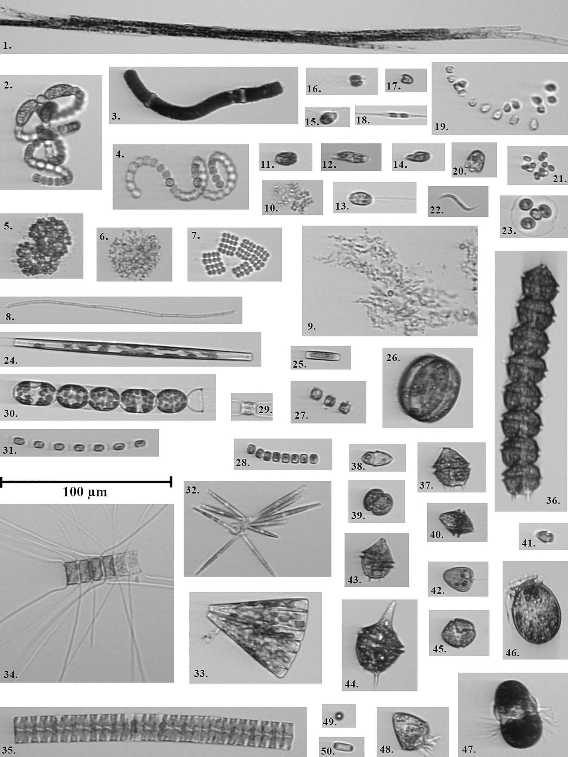
Figure 1 Example images representing the classes. 1) Aphanizomenon flosaquae, 2) Dolichospermum sp./Anabaenopsis sp. coiled, 3) Nodularia spumigena, 4) Dolichospermum sp./Anabaenopsis sp., 5) Snowella sp./Woronichinia sp., 6) Chroococcales, 7) Merismopedia sp., 8) Oscillatoriales, 9) Aphanothece paralleliformis, 10) Chroococcus sp., 11) Eutreptiella sp., 12) Euglenophyceae, 13) Cryptomonadales, 14) Cryptophyceae/Teleaulax sp., 15) Katablepharis remigera, 16) Pseudopedinella sp., 17) Pyramimonas sp., 18) Ceratoneis closterium, 19) Uroglenopsis sp., 20) Cymbomonas tetramitiformis, 21) Chlorococcales, 22) Monoraphidium contortum, 23) Oocystis sp., 24) Pennales thin, 25) Pennales thick, 26) Centrales, 27) Thalassiosira levanderi, 28) Cyclotella choctawhatcheeana, 29) Chaetoceros sp. single, 30) Melosira arctica, 31) Skeletonema marinoi, 32) Nitzschia paleacea, 33) Licmophora sp., 34) Chaetoceros sp., 35) Pauliella taeniata, 36) Peridiniella catenata chain, 37) Peridiniella catenata single, 38) Gymnodiniales, 39) Gymnodinium like cells, 40) Heterocapsa triquetra, 41) Heterocapsa rotundata, 42) Prorocentrum cordatum, 43) Gonyaulax verior, 44) Amylax triacantha, 45) Dinophyceae, 46) Dinophysis acuminata, 47) Mesodinium rubrum, 48) Ciliata, 49) Beads, 50) Heterocyte.

The SYKE-plankton_IFCB_2022 data set was collected in the Baltic Sea on different occasions, to cover spatio-temporal variations in plankton communities. In 2016 and 2019 water samples (n=52) were collected using the Alg@line ferrybox systems of M/S Finnmaid and Silja Serenade (Ruokanen et al., 2003; Kaitala et al., 2014) and analyzed in the laboratory with the IFCB. In 2017 and 2018 data were collected at the Utö station over the deployment periods, with the continuous set up of the IFCB, followed by the sporadic selection and labeling of a set of samples (n=62) (Figure 2).

FIGURE 2

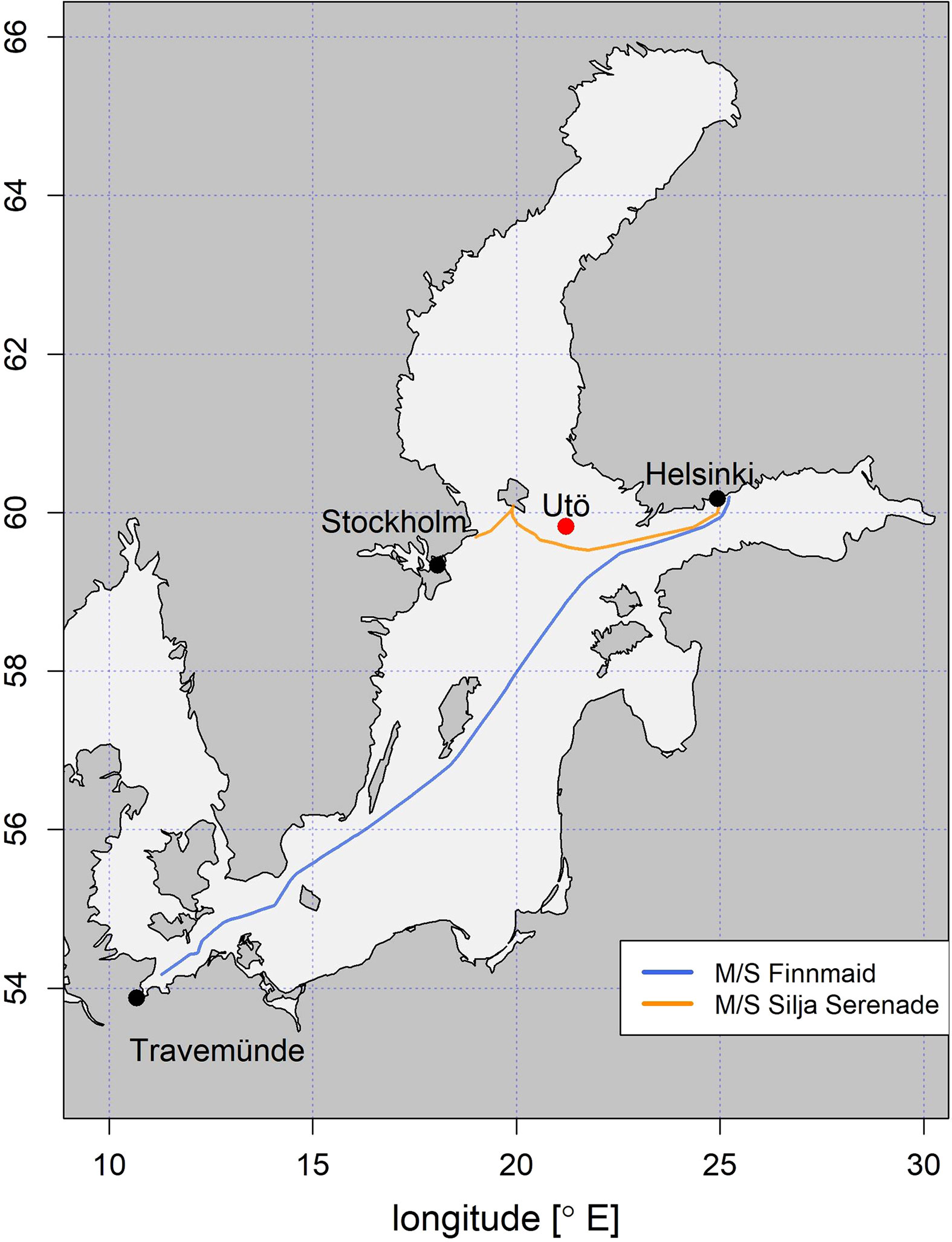
Figure 2 Map showing the location of Utö Atmospheric and Marine Research Station, and the points along the Alg@line routes of M/S Finnmaid and M/S Silja Serenade, from where the manually annotated samples were collected.

Images of natural phytoplankton communities reflect their wide morphological diversity, resulting in large variations in size and aspect ratios of the images, with images ranging from tens to hundreds of pixels vertically and tens to more than one thousand pixels horizontally. The samples were labeled using a tool created by Sosik et al. (https://github.com/hsosik/ifcb-analysis/wiki/Instructions-for-manual-annotation-of-images). Some samples were labeled so that all identifiable regions of interest (ROIs) were assigned to a class and some samples were labeled only partially, to expand the labeled sets of some classes. The data set, therefore, does not represent real-life proportions among classes, however, the number of images per class still reflects, to some extent, their prevalence in natural populations.

The IFCB produces a non-negligible amount of images that are difficult or even impossible to identify with certainty. To train a CNN model, only images that can be reliably labeled should be used, to avoid mislabeled images which would negatively affect the training process. However, for testing the performance of the model, the unidentifiable part of the samples should be considered for calculating realistic performance metrics. The SYKE-plankton_IFCB_2022 data set was divided using stratified sampling, into training, validation and test sets (60%, 20% and 20% respectively). The training set, referred to here as Training Data, was used exclusively for training the model. The validation set had two purposes. First, it was used to monitor the model’s accuracy during training, which is what it is usually used for, and in this sense is referred to as a validation set. After the model training was complete, the validation set was complemented with an equal number of unclassifiable images (50-50%) to make it more representative of image data from natural phytoplankton communities (including detritus and other unidentifiable images). The validation set complemented by the unidentifiable images (Validation Data) was used to determine class-specific thresholds which will be explained in section 2.3.1 Probability filtering of unclassifiable images using thresholds. For the same reason as with the Validation Data, the test set was similarly complemented with equal numbers of unclassifiable images (50-50%). The test set with unclassifiable images (Test Data) was used to calculate the final, unbiased estimation of the model’s performance. The difference between dominant and rare taxa in the SYKE-plankton_IFCB_2022 data set manifests itself as a large imbalance in the number of images per class: it varies from 19 (Amylax triacantha) to 12 280 (Dolichospermum sp./Anabaenopsis sp.).

2.2.2 Image data set for performance evaluation

As previously explained, correct evaluation of model performance in classifying natural samples requires test data to contain difficult-to-classify images. That is, their features fit several different classes (so-called borderline images), as is the case with multiple images in natural samples. For this purpose, 59 samples were selected from 2021 when the IFCB was continuously deployed in Utö; first as one per week throughout the year complemented with samples from specific seasons to target specific classes. All samples were manually labeled in their entirety so that each image was assigned to one of the 50 classes or as “unclassified” (unable to be assigned to any of the existing classes). The image labeling was done with a custom graphical tool in a Jupyter Notebook, utilizing the model's predictions to speed up the process. This data set, SYKE-plankton_IFCB_Utö_2021 (Evaluation Data), is publicly available at http://doi.org/10.23728/b2share.7c273b6f409c47e98a868d6517be3ae3.

2.3 The CNN model

The neural network model used in this study is based on a pre-trained ResNet-18 (He et al., 2016) and fine-tuned with the SYKE-plankton_IFCB_2022 Baltic Sea phytoplankton image data set, described above. The pre-trained model was obtained from TorchVision, which is part of the PyTorch project (Paszke et al., 2019). TorchVision models are pre-trained on the ImageNet data set (Deng et al., 2009), which consists of RGB images of 1000 classes, such as fire truck and Golden Retriever. The head of the pre-trained ResNet-18, i.e., the last fully connected linear layer, was replaced with three new linear layers, while the rest of the network layers were only fine-tuned. The new layers were initialized with the default PyTorch initialization for linear layers, which was in more detail a uniform distribution between -√k and √k, where k = 1/in_features.

To improve the performance of unseen images (not present in the Training Data), avoid overfitting and reduce class imbalance, first, random oversampling was done for the smaller classes in the Training Data so that each class contained a minimum of 100 training images. Secondly, some simple image augmentations were used for all classes in the Training Data (including the resampled images): horizontal and vertical flip, translation, zoom and brightness change. However, all augmentations were done sparingly since images generated by the IFCB are quite homogeneous. More specifically, translation was done only on the shorter side of the original image and none of the original pixels were clipped, the zoom range was 0.6 to 1.4, the rotation range was -10 to 10 degrees, and the range of brightness change was 0.95 to 1.1. Another approach to address class imbalance would be to provide class-specific weights to the optimizer (see e.g. cost-sensitive learning, Thai-Nghe et al., 2010). However, to avoid reducing the generalizability of the model to data sets with different class proportions, this method was not used.

Images were resized to 180×180 pixels since 180 is the mean width of the training images. To preserve the original image aspect ratio, the mode (i.e., most frequent) pixel value of each image was used as padding in its resized form. Pixel values were scaled between 0 and 1 for each image, a process known as min-max normalization, to avoid any training overhead caused by unnecessarily large integer values. Although the IFCB images are grayscale, because the original ResNet was trained with RGB images, three color channels were used.

A categorical cross-entropy loss was used with Adam as the optimizer function (Kingma and Ba, 2014). To further improve model training, a custom learning rate schedule was used. This schedule consisted of three steps. At each step, the number of trainable layers was increased, and the learning rate was decreased. Step 1 lasted for 5 epochs, where only the last linear layers were trained with a learning rate of 0.01. Step 2 lasted for the next 10 epochs, where the training of the last convolutional layer was started with a learning rate of 0.001, and the learning rate of the linear layers was decreased to 0.005. Step 3 lasted from epoch 16 onward, where the rest of the base layers were trained with a 0.0001 learning rate, the last base layer was trained with 0.001, and the head layers were trained with 0.0025. The training was stopped when the loss value on the validation set did not decrease for 12 epochs. The average training time was one hour on a single NVIDIA Tesla P100 GPU.

Class-specific recall, precision and F1-score were calculated for the classification results to describe the class-specific performance of the model. The weighted average F1-score was calculated to describe the entire model performance since global accuracy is a flawed metric for class-imbalanced data (Hossin and Sulaiman, 2015). Weighted average F1-score was chosen since we were evaluating the classification model from an operational point of view, in which case, the common classes and therefore more abundant ones should be given more weight. The computation involves True positive (TP), False positive (FP) and False negative (FN) numbers. Recall quantifies how well classes are identified and is computed as the proportion of successful identifications in a class. Precision quantifies how well other classes are rejected and is computed as the proportion of positive identifications that were correct. F1-score expresses the balance between recall and precision.

$$\text{Recall}=\left(\text{TP}/\left(\text{TP}+\text{FN}\right)\right)$$

$$\text{Precision}=\left(\text{TP}/\left(\text{TP}+\text{FP}\right)\right)$$

$$\text{F}1-\text{score}=\left(2*\left(\left(\text{precision}*\text{recall}\right)/\left(\text{precision}+\text{recall}\right)\right)\right)$$

2.3.1 Probability filtering of unclassifiable images using thresholds

As explained before, not all images captured by IFCB are classifiable due to a lack of characteristic features for example. We chose not to create classes for those. Therefore, a filtering method was needed to remove those images when the CNN was deployed. For each image, a classifier produces prediction scores for all classes in the training data. Prediction scores can be considered the probability of correctly classifying an image and the highest prediction score represents the winning class. By assigning a threshold, which the prediction score must exceed, they can then be used to filter out images with low classification probabilities. The threshold is not universal but class-specific. Therefore a unique probability threshold was estimated for each class, and only images with at least one class probability above any assigned thresholds were assigned to a class. Filtering the data is a proven method to treat low probability classifications (Faillettaz et al., 2016; Luo et al., 2018).

The final layer in our CNN model uses a softmax activation function, which outputs a normalized probability distribution over the classes. Since the probability distribution coming from a softmax can be quite extreme, i.e., one class has most of the probability mass, the outputs from the layer before the softmax were scaled down. Scaling was done by multiplication by the natural logarithm of 1.3. This has the same effect as changing the base of the exponents in the softmax function from e to 1.3, however, it is easier to scale the outputs rather than modify the softmax itself. The value of 1.3 was determined by manually testing different values. In short, the conversion is: softmax(out×ln(1.3)), where out = the outputs of the layer before softmax. This conversion introduced more smoothness in the class probabilities while maintaining their order (and therefore the classification). Smoothness made it easier to set class probability thresholds. A figure illustrating the effect of scaling on selected ROIs can be found in the supplementary material (Supplementary 3).

Ideally, thresholds would be assigned with a data set representing a species distribution similar to that of a natural community. However, the community composition changes with the seasons and species dynamics differ from year to year. Therefore, acquiring an ideal data set for threshold determination, which represents natural distribution covering all common species, is laborious. To start the implementation of the classifier we used the Validation Data to determine thresholds. The Validation Data was run through the classifier and precision, recall and F1-score were calculated. The threshold was varied and the value yielding the highest F1-score was chosen for a given class. The chosen thresholds were tested by running the Test Data through the classifier, and precision, recall and F1-score were calculated. Images below the thresholds were still considered when calculating performance metrics: correct images of a class which reached the assigned threshold limit were considered as TP and incorrect images FP; correct images below the threshold limit were considered as FN and incorrect images TN.

The code implementing the model described above can be found at https://github.com/veot/syke-pic.

2.4 Data transfer and services

First, the IFCB data is stored on the instrument’s hard drive. Then the IFCB is connected to the Utö station’s inner network, through which the data flows to the Finnish Meteorological Institute (FMI) file server via optical fibre, where it is temporarily stored. From there onwards it is transferred to a cloud object storage service Allas, provided by the Finnish IT Center for Science (CSC). Allas is based on CEPH object storage technology, allowing to easily share data to other services within the CSC’s computing platform - much like Amazon S3 in AWS. The subsequent data analysis (described below) is done on a Linux virtual machine with 6 vCPUs and 16 GB of memory (the number of resources required for computing also image biovolumes, described below), also provided by CSC. Significantly fewer resources are needed when running the CNN-classifier alone.

2.5 Near-real-time data analysis

To use the generated IFCB images and the CNN classifier for near-real-time phytoplankton monitoring, a basic data pipeline was established. The near-real-time data pipeline and classification system were taken into use at the beginning of summer 2021. The entire data transfer pipeline results in a total delay of about two hours from the image capture to the point when the image is classified. The classification is performed automatically via the above-described CNN model as soon as a new batch of IFCB data is updated to Allas, on an hourly schedule, and the data is classified into the 50 classes. In addition to image classification also image-specific biovolumes are computed. A method developed by Moberg and Sosik (2012) is used for computing the biovolumes of the objects (phytoplankton) in the images taken with IFCB. More detailed descriptions of available MATLAB-based tools and open access codes can be found at https://github.com/hsosik/ifcb-analysis. For comparison of the biovolume estimates with those obtained via traditional phytoplankton monitoring methods of the Baltic Sea area (HELCOM, 2017), the biovolumes are converted to biomass (µg L^-1) assuming a plasma density of 1 g cm^-3 (CEN, 2015). Finally, the biovolume/biomass information is combined with the classifications resulting in a usable form of class-specific biovolume/biomass per L in a sample and the hourly mean is calculated.

2.6 Evaluation of the near-real-time classifier system

To assess how well the model classified natural samples using the thresholds determined using the Validation Data, a total of 59 samples (a total of approx. 20 hours of data) were selected from data collected with IFCB between January to December 2021 (the Evaluation Data). First the selection targeted one sample per week, but due to the scarcity of some classes additional samples were selected from expected seasons to find images of the scarce classes. As proposed by González et al. (2017) for proper performance validation a set of samples should have sufficient variability. We attempted to ensure this by selecting samples from different seasons which also covered transition phases. Selected samples were manually inspected: all classifications were assessed (confirmed or corrected) and all identifiable images which fell below the thresholds were labeled. The unidentifiable images left without an assigned class were considered unclassified. Unclassified images are still accounted for in the total community biomass with the assumption that when chlorophyll a is used as a trigger the majority of imaged particles should be living material. The TP, FP and FN were counted and consequently precision, recall and F1-score were calculated for each class. Class-specific metrics were calculated based on the thresholds determined using the Validation Data, so images below the thresholds were still taken into account: correct images within a class to reach the assigned threshold were considered TP and incorrect images FP; correct images below the threshold were considered FN and incorrect images TN.

3 Results

3.1 CNN classifier performance

The first step in implementing a near-real-time analysis of plankton communities is to establish a suitable recognition model. Overall classification performance of the Test Data using CNN was high (F1-score 0.95), and the network was able to identify many common species of the Baltic Sea phytoplankton community. The class-specific precision, recall and F1-score were between 0.85 and 1 in over half of the classes, but some of the classes had much lower values (0.4-0.6) (Table 1).

TABLE 1

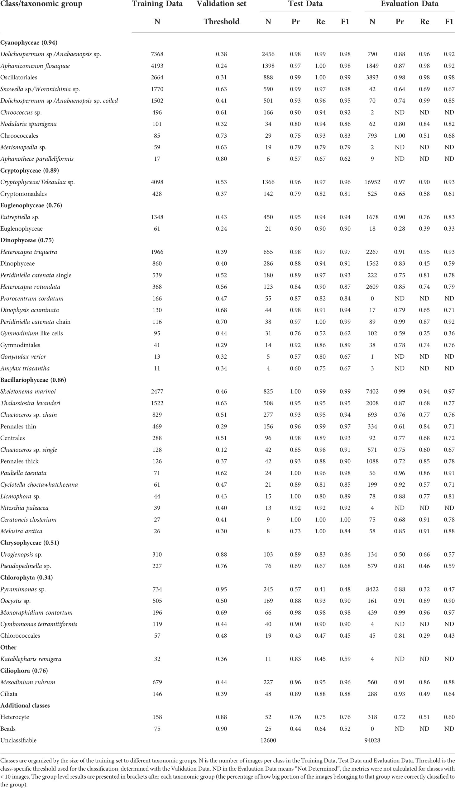
Table 1 The table represents the class-specific classification metrics for the Test Data and for the Evaluation Data (Pr, precision; Re, Recall; F1, F1-score; N, number of images).

With classes having the largest training sets (> 1000 images), all the metrics (precision, recall and F1-score) were between 0.94 - 1. With some classes such as Euglenophyceae, Dinophysis acuminata, Peridiniella catenata chain, Ceratoneis closterium, Nitzschia paleacea, Monoraphidium contortum and Cymbomonas tetramitiformis all the metrics were > 0.9, although the Training Data contained < 200 images. Classes with the poorest performance (all metrics < 0.7) were Aphanothece paralleliformis, Pseudopedinella sp., Pyramimonas sp., Chlorococcales and Beads (calibration). These all contained low numbers of training images (17 – 227, discounting data augmentation) except for Pyramimonas sp. (734 images). The largest differences between precision and recall were found with the classes, Gymnodinium like cells (0.76, 0.52), Gonyaulax verior (0.57, 0.8), Melosira arctica (0.73, 1), Katablepharis remigera (0.83, 0.45) and Beads (0.44, 0.64). With Gymnodinium like cells and Katablepharis remigera precision was higher than recall, meaning rejection of images not belonging to the class was higher than recognition of images which did belong to the class. For the classes Gonyaulax verior, Melosira arctica and Beads, there was no issue in recognizing the images belonging to the class, however, there was the problem of a high proportion of false positives. Metrics for classes of filamentous cyanobacteria (an important group in the Baltic Sea) were all ≥ 0.93 except for the class, Nodularia spumigena, which had the poorest performance (0.8 – 0.94). It is important to note that Nodularia spumigena’s training set had a considerably smaller number of images (only 101, compared to Aphanizomenon flosaquae: 4193, Dolichospermum sp./Anabaenopsis sp.: 7368, Dolichospermum sp./Anabaenopsis sp. coiled: 1502) (Table 1).

When applying the classification system (the Evaluation Data) overall performance dropped, but remained fairly high for natural samples (F1-score 0.82). All class-specific classification metrics are presented in Table 1. For the classes with > 1000 images in the Training Data, the change in F1-score was ≤ 0.1 except for the classes, Snowella sp./Woronichinia sp., Eutreptiella sp. and Thalassiosira levanderi. For classes with < 200 images in the Training Data score decreased ≤ 0.1 for Nodularia spumigena, Peridiniella catenata chain, Pauliella taeniata, Licmophora sp., Melosira arctica and Monoraphidium contortum. The F1-score of Melosira arctica increased along with a larger number of images, on which the evaluation was based (8 in the Test Data and 58 in the Evaluation Data). The results for classes with < 10 images in their Evaluation Data will not be presented as these rare occurrences would not help in analyzing the model performance. However, classes with < 10 images in their Test Data were presented, as some classes had much higher number of images in the Evaluation Data (Melosira arctica and Ceratoneis Closterium). Other classes with > 10 images in the Evaluation Data, the poorest performance (metrics < 0.7) was found for classes Snowella sp./Woronichinia sp., Cryptomonadales, Gymnodinium like cells, Uroglenopsis sp. and Heterocyte. The recall and F1-score (0.29 – 0.59) were low for the classes Pseudopedinella sp., Pyramimonas sp. and Chlorococcales but precision was relatively high indicating a poor function in class recognition and that class-specific thresholds should be adjusted. Class recognition performance of filamentous cyanobacteria (Aphanizomenon flosaquae, Dolichospermum sp./Anabaenopsis sp., Dolichospermum sp./Anabaenopsis sp. coiled, Nodularia spumigena) was relatively high. This was also true for natural samples (F1-scores 0.82 – 0.92) (Table 1).

The majority of classification problems, of course, occurred between classes which resembled one another and were typically from closely related taxa. The highest confusion amongst CNN model results, when probability filtering thresholds were not used, were within different classes of dinoflagellates and between species-level classes and higher taxonomic-level classes belonging to the same order (Table 2). Gymnodinium like cells were confused (35%) for Dinophyceae and placed within a higher taxonomic branch, Amylax triacantha and Gonyaulax verior (with 4 and 5 images in the Test Data respectively) were confused (25% and 20% respectively) for Peridiniella catenata single (539 training images). Chlorococcales was also considerably confused for Oocystis sp. (26%). From filamentous cyanobacteria, only 6% of Nodularia spumigena was confused with Aphanizomenon flosaquae (Table 2). A confusion matrix with all confused classes is provided as supplementary material (Supplementary 1).

TABLE 2

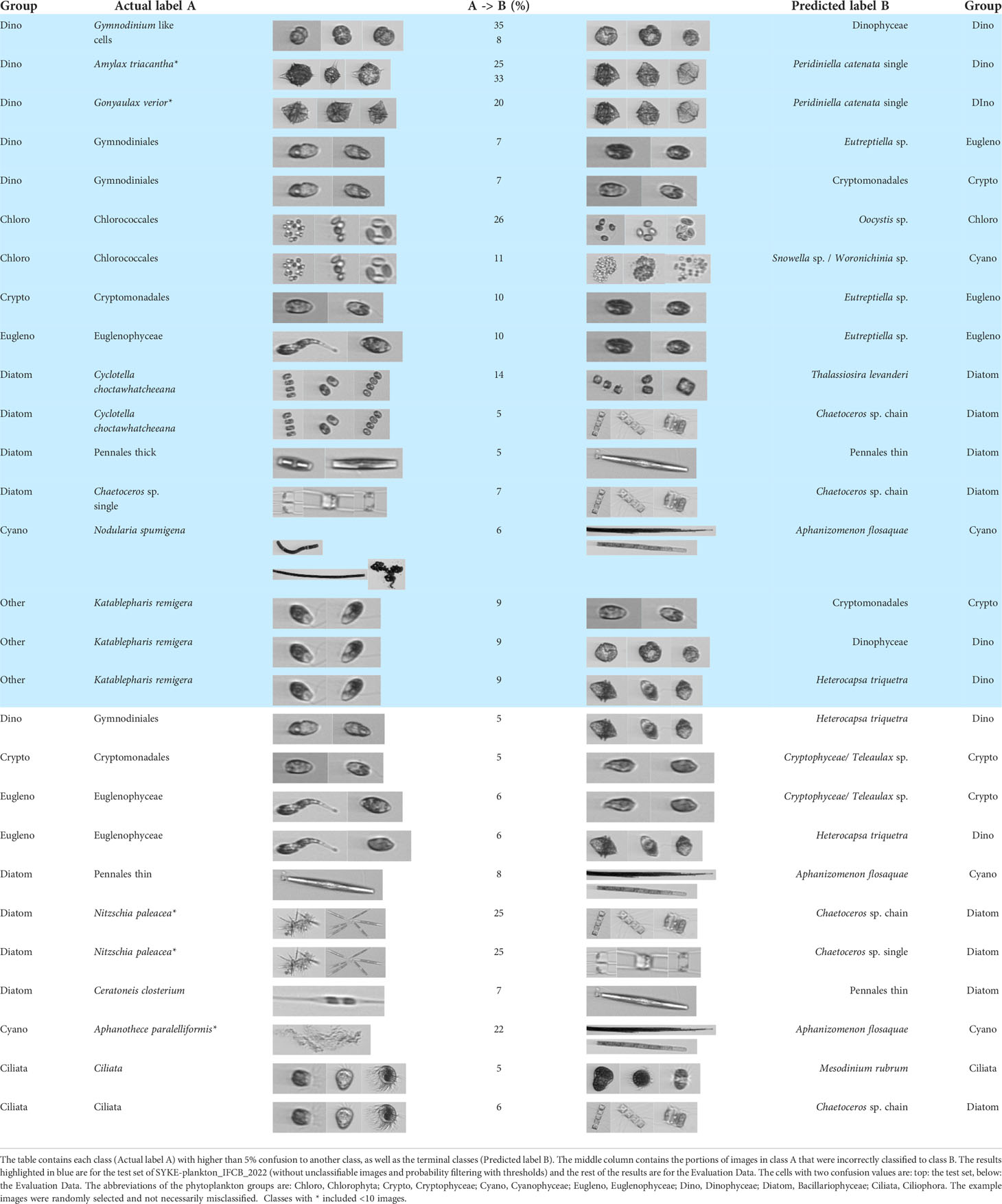
Table 2 Class pairs with the highest number of inter-class classification errors.

Confusion was lower among classes in the Evaluation Data when probability filtering with thresholds was applied. However, several images were left unclassified, as a delicate balance between TP and FN must be achieved for threshold assignation. A class-specific confusion matrix for the Evaluation Data, including those left unclassified, is provided as supplementary material (Supplementary 2). Similar, to the Test Data without filtering, the highest confusion among classes in the Evaluation Data was mainly between classes of close taxonomic relation. The highest confusion occurred (> 15%) between classes with < 10 images of data. Therefore, drawing any conclusion should be done very scarcely. What can be said reliably, is that classes with a small amount of training data are easily confused with classes similar in morphological appearance. Otherwise, the confusion rates were very moderate (5 – 8%) (Table 2).

When looking at confusion at the level of broader taxonomic groups there was practically no confusion between different groups (Figure 3). However, the proportion of images left unclassified due to probability filtering with thresholds varied greatly. Groups with the best identification rates, and with the least unclassified images, were Cyanophyceae, Cryptophyceae and Bacillariophyceae (6%, 11% and 13% respectively). For the classes, Euglenophyceae, Dinophyceae and Ciliophora, a reasonable proportion of images were left unclassified (22%, 24% and 19% respectively). Chrysophyceae and Chlorophyta had the highest proportion of unclassified images (49% and 65% respectively) (Figure 3).

FIGURE 3

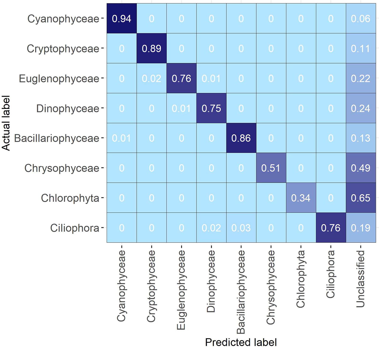
Figure 3 Confusion matrix of the Evaluation Data aggregated on broader taxonomic group level.

3.2 Implementation of a near-real-time phytoplankton community information system

The operability and utility of the near-real-time data processing pipeline were used in the summer of 2021, as a demo, for up-to-date information on the abundance of the three bloom-forming cyanobacteria taxa of the Baltic Sea (with approx. 2h delay between sampling and online publication of classified results) (Figure 4). A simple visualization of the cyanobacteria situation was created and published online (“Cyanobacteria biomass” in https://swell.fmi.fi/hab-info/) to ensure public accessibility of the prevailing situation. The visualization shows a continuously updated graph containing information on the biomass of three main bloom-forming cyanobacteria taxa. This biomass graph was used, as an indicator of the predominant taxa off the coast of Finland, in SYKE’s weekly cyanobacterial reports in summer 2021 (https://www.syke.fi/en-US/Current/Algal_reviews).

FIGURE 4

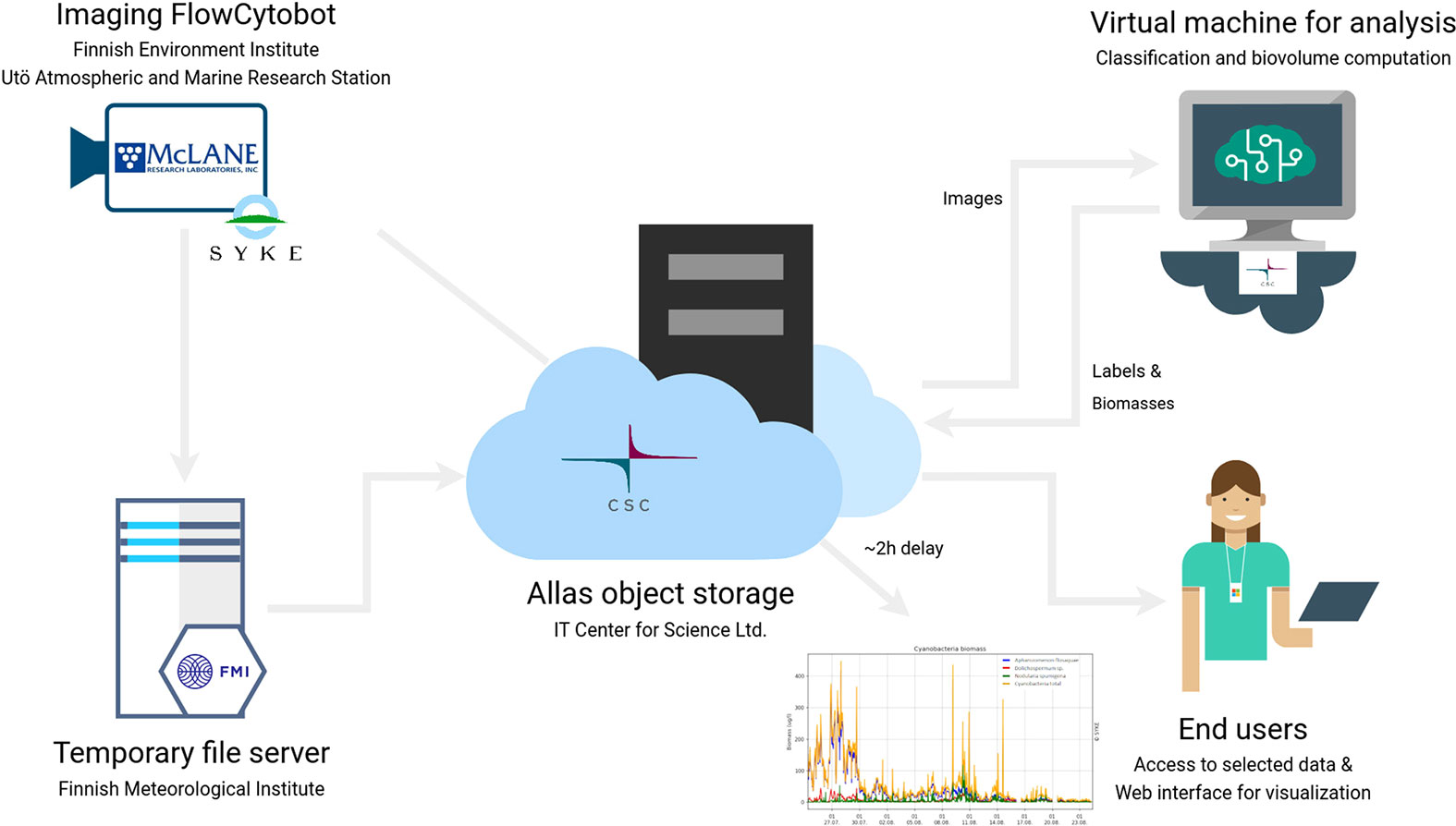
Figure 4 Scheme of the automated data flow and the subsequent data processing pipeline.

Dolichospermum sp./Anabaenopsis sp. started to bloom in late June, quickly achieving high biomass (peak in ~500 µg L^-1 on July 2) followed by a quick drop within a few days. While Dolichospermum sp./Anabaenopsis sp. biomass was on the decline, Aphanizomenon flosaquae biomass started to increase, reaching its peak (~400 µg L^-1) within approximately five days (on July 5). A. flosaquae achieved a lower biomass peak but was spread over a longer period than that of Dolichospermum sp./Anabaenopsis sp. A secondary and smaller peak (~150 µg L^-1) appeared later in July (19^th/20^th) and was caused by both Dolichospermum sp./Anabaenopsis sp. and A. flosaquae. A. flosaquae formed a third peak at the end of July reaching a biomass of ~400 - 500 µg L^-1. Nodularia spumigena was detected, sporadically more abundant in some samples but did not exhibit a consistent biomass increase (Figure 5A). Although it was the cyanobacterial bloom season, the total filamentous cyanobacteria biomass constituted only approx. a third of the total phytoplankton community biomass. Simultaneously to the decline of the first cyanobacteria peak, the phytoplankton community’s total biomass increased (Figure 5B). The third cyanobacteria peak achieved a similar magnitude as the second peak, but with differing community composition, demonstrating the importance of obtaining more detailed, higher-resolution information on community composition (Figures 5A, B).

FIGURE 5

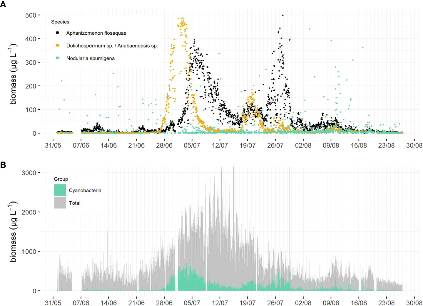
Figure 5 The biomasses of the three bloom forming filamentous cyanobacteria taxa of the Baltic Sea in summer 2021, black = Aphanizomenon flosaquae, orange = Dolichospermum sp./Anabaenopsis sp., green = Nodularia spumigena (A). The total phytoplankton community biomass (grey) and the total filamentous cyanobacteria biomass (green) from the same period (B). The data was classified with the automated CNN model in near-real time.

4 Discussion

Recently plankton imaging systems have become numerous, diverse and widely used (Lombard et al., 2019). The classification of plankton images has become popular resulting in multiple publications and classification algorithms, often focusing on CNN applications (see e.g. Dunker et al., 2018; Luo et al., 2018; Lumini and Nanni, 2019; Kerr et al., 2020; Lumini et al., 2020; Guo et al., 2021; Henrichs et al., 2021; and the references therein). This popularity is due to the great need for efficient solutions for automated analysis and data flows of the vast amounts of image data produced, and underlines the importance of the quality of the data products (Muller-Karger et al., 2018).

However, papers on plankton classification often report only the classification performance and do not account for its practical implications on aquatic research, such as the effect of confused classes and classification processes from an operational point of view (e.g. Orenstein and Beijbom, 2017; Bureš et al., 2021). In transitioning to more frequent use of these new instruments it is important to focus on the steps needed for operationality and reference them with traditional light microscopy (Haraguchi et al., 2017; Kraft et al., 2021) as well as combining the two methods, as different methods confer different advantages. Between-sensor studies are scarce, nevertheless, in future, they will be sorely needed.

We demonstrated in this paper the functionality of CNN in classifying IFCB images from the Baltic Sea. Furthermore, we developed a framework for near-real-time image classification, which is sorely needed in HAB observations and also supports the future development of operational modelling and remote sensing applications. We provided a practical example with near-real-time observations of the summer cyanobacteria blooms, a reoccurring nuisance for users of the Baltic Sea. The species composition, timing and magnitude of the blooms are difficult to predict as controlling factors are still something of a puzzle (Kahru and Elmgren, 2014; Kownacka et al., 2018; Kahru et al., 2020). The summer of 2021, for example, was atypical (Figure 5) and the highest biomass peaks were only half that of the peaks recorded during an intensive bloom in 2018 (Kraft et al., 2021). The three major bloom-forming taxa in the Baltic Sea are Nodularia spumigena, Aphanizomenon flosaquae and Dolichospermum spp. (Niemistö et al., 1989; Stal et al., 2003; Olofsson et al., 2020), of which only A. flosaquae is not known to be toxic. Therefore, the separation of these three taxa in the Baltic Sea environment is highly important, which was already achieved (Table 1, Supplementary 2).

Though this paper is not about the study of ecological phenomena, two observations highlighting its future potential are worth mentioning. First, even during the filamentous cyanobacteria bloom peaks, their biomass was a third of the total phytoplankton biomass (Figure 5B). Second, while the total cyanobacteria biomass was of the same order of magnitude during the second and third peaks, the species composition differed, with the second peak consisting of approximately equal parts of two taxa, Dolichospermum sp./Anabaenopsis sp. and Aphanizomenon flosaquae, and the third peak almost solely of the latter. These observations, as well as the variability of the overall phytoplankton species composition, will be considered in a more ecologically focused follow-up study. However, it demonstrates that the utilization of new automated methods, such as imaging flow cytometry, plays a key role in deepening our understanding of these bloom processes (Kraft et al., 2021). Yet, these measurements must be made in conjunction with physical and biogeochemical observations, using the same observation platforms, such as the one at Utö (Laakso et al., 2018; Honkanen et al., 2021; Kraft et al., 2021).

Before digging into the ecology behind these phenomena, there are still a few practical aspects to be considered from an operational point of view. First is the classification model performance. The level of performance must be adequate to enable utilization of the results and verification of these results needs to be done for natural samples to ensure adequate performance during operational use. Second is the implications of confused classes. Some confusion doesn’t mean the results are unusable, but a proper aggregation level needs to be selected, otherwise, the results of only certain classes that meet the user’s criteria should be used. Third, some practical decisions on how to deal with the large number of difficult-to-assign images should be made. There is a lot of work to be done before the plankton classification problem is solved and data collected during the meantime needs to be harnessed while development continues.

4.1 Classification model performance

Overall, the CNN model used for classification in this study performed very well, although there was some class-specific variation in the classification scores (Table 1). The overall F1-score for the Test Data was 0.95. This can be considered highly accurate and is on par with the results obtained in recent phytoplankton studies (Lumini and Nanni, 2019; Lumini et al., 2020; Walker and Orenstein, 2021). There was a drop in performance when using the classifier in operational mode (the overall F1-score for the Evaluation Data was 0.82). Recht et al. (2019) found that the accuracy of models tends to drop even when tested with data created to match the training data’s distribution profile. This is due to human labeling subjectivity which makes it impossible to produce the same distribution. They concluded that the models are insufficient for generalization to more difficult images e.g. absence or deficiency of necessary features in the image. In our case, this drop may partly be due to the different distribution of training images compared to the target data and is partly explained by the inferior performance of some classes. Similar to the conclusions of Recht et al. (2019), the drop in our case is probably largely due to the large number of so-called borderline cases in natural samples, which make them difficult to classify. This makes the decision on where to draw the line difficult and leads to a high number of both FP and FN.

The drop, when applying the classifier during operational use, was in either precision or recall, or both. In many cases, the drop was larger with precision than recall meaning that the thresholds applied to those classes should be adjusted downward. Also, in many cases, the drop in recall was higher than that of precision meaning that thresholds for those classes should be adjusted upward. This proves the importance of threshold selection and although our results indicate that Validation Data is adequate for setting initial threshold values, it does not provide optimal thresholds as the borderline images are missing from the Validation Data. However, threshold adjustment is done cumulatively based on operational data such as is collected at Utö and they need to be adjusted and refined as data and information is accumulated. After adjusting the threshold values, it is not a heavy task to compute the previous time series using the new threshold values since the predictions have already been done.

In our study, we included some classes with only ~20-70 images per class and still reached relatively high classification metrics with the Test Data for some of those classes (Table 1). This is partly explained by the efficient data augmentation methods, as supported by the results of e.g. Correa et al. (2017) and partly by the unique morphology/appearance compared to other classes (Figure 1). However, those classes (except Pauliella taeniata and Melosira arctica) experienced a noticeable drop or didn’t contain sufficient occurrences for the proper estimation of performance when classifying the Evaluation Data (Table 1). In the case of Ceratoneis closterium, Licmophora sp. and perhaps Cyclotella choctawhatcheeana this may also be a need for adjusting the class-specific thresholds since there was a relatively high difference between their precision and recall. Although it is possible to increase the training set of classes with low numbers of images using data augmentation, the classification results cannot be considered reliable when they are based on only few images e.g.< 10 images.

The classification score improved when more images were available in the Training Data, with a greater improvement for classes containing > 2000 images. All classes with large training sets had an F1-score > 0.9 for both the Test Data and the Evaluation Data. Although more images in the training set seem to be advantageous, there were also several classes (Nodularia spumigena, Peridiniella catenata chain, Pauliella taeniata, Licmophora sp., Melosira arctica and Monoraphidium contortum) with relatively good F1-scores (> 0.8) even with< 200 images in the training set. This would imply that distinguishable features (e.g. a specific shape) strongly influence the successful identification of specific classes amongst those with less labeled images (Figure 1, Table 1).

4.2 Class-specific confusion and its practical implications

Characteristic features of an organism tend to lead to a more accurate classification of images, however, many common Baltic Sea phytoplankton species, such as dinoflagellates, do not have obvious distinguishable features in their IFCB images which could be used to differentiate them. Consequently, those cases which were most confused were among classes of dinoflagellates (Table 2). Confusion within classes closely related taxonomically, such as classes on a higher and lower level of the same taxonomic hierarchy or different species belonging to the same order (Oocystis sp. and Chlorococcales, Eutreptiella and Euglenophyceae, Mesodinium rubrum and Ciliata, Cyclotella choctawhatcheeana and Thalassiosira levanderi, Nodularia spumigena and Aphanizomenon flosaquae) were usually due to those classes being very similar in appearance (Table 2). The same holds for other types of flagellates, e.g., classes Cryptomonadales and Euglenophyceae. Similar results have also been found by Sosik and Olson (2007), but it is difficult to compare our findings to the literature as class-specific confusion is usually not presented, let alone discussed. In many cases of confusion, the class differentiated with fewer training images was confused with a class differentiated by a large training image set with a close morphological resemblance. This emphasizes the power of larger training sets (Table 1, Table 2). This is a common problem with imbalanced data sets as the trained classifiers tend to be biased towards more numerous classes (Johnson and Khoshgoftaar, 2019).

Confusion of classes does not always create a major problem. In some cases, it is sufficient to simply achieve group-level identification. However, this must be carefully evaluated for research topics which require species discrimination. If the focus is on the identification of phytoplankton functional groups, it may be sufficient to determine which groups of plankton, e.g. dinoflagellates or diatoms, dominate the community. However, group-level differentiation is insufficient if we are interested in determining the biodiversity or whether toxic species are present. Group-level identification means that the results of classes closely related taxonomically, such as the Eutreptiella sp. and Euglenophyceae, can be united without having a practical impact. Looking at our classification results on a broader taxonomic group level it is evident that the results are reliable, at least for some groups. For the groups, Cyanophyceae, Cryptophyceae, and Bacillariophyceae 86 – 94% of the images were correctly classified, and for Euglenophyceae, Dinophyceae and Ciliophora 75 – 76% were correctly classified. For Cryptophyceae and Chlorophyta, less than 50% of the images were correctly identified and there was high uncertainty limiting the ability to make conclusions about their presence and abundance (Table 1, Figure 3). Confusion between groups was minor and incorrectly classified images were usually assigned to the unclassified group due to thresholding (Figure 3). It is always best to determine community composition down to the lowest taxonomical level possible. This is also desirable when using automated classification systems, especially when it is possible to identify them visually.

4.3 Towards operationality

Though often considered superior to other methods, CNNs are still not widely utilized for classifying and analyzing natural phytoplankton data sets. While the deep feature extraction outperforms handcrafted features, the latter performs well for several phytoplankton groups originally classified with both SVM and RF-based classifiers (Sosik and Olson, 2007; Laney and Sosik, 2014; Anglès et al., 2015; Bueno et al., 2017; Anglès et al., 2019; Fischer et al., 2020; Kraft et al., 2021). Currently, most ecological studies using phytoplankton data sets collected with an IFCB base their classification on the features and method developed by Sosik and Olson (2007) using RF instead of SVM. One reason for this is that CNNs typically require a long training time, high computing power and many training images, requiring more time and effort to establish an operational classification system. Additionally, publicly available codes and workflow are accessible for the RF-based classifier system, thus making it easier for biologically oriented groups to begin establishing new classifier systems (https://github.com/hsosik/ifcb-analysis).

CNNs require a notable amount of computational resources especially if they are trained from scratch. We showed that even relatively shallow CNN model requiring only a quite basic level of computing power with a small number of training data (26 classes out of 50 contained less than 300 training images) performs well. Previous studies support these findings (Bureš et al., 2021). During operational mode (the Evaluation Data), classification performance dropped drastically for many of the classes with few training images. However, 12 of those also achieved an F1-score of 0.7-0.97. This suggests not all classes require extremely large training sets, speeding up the process.

Creating the training sets in and of itself is laborious. It is therefore impractical to create classes for images of all small objects of similar shapes, such as different types of detritus and other types of difficult-to-assign objects. The creation of classes for such images will lead to too many variations in appearance. This will result in the matching of such images to other classes with similar features causing confusion. Hence we chose not to classify such images, but used thresholds instead. However, there is some benefit to creating classes for certain types of detritus as it allows them to be filtered out from the total community biomass. On the other hand, this leads to questions such as when should a phytoplankton cell be considered detritus, considering that all images have been triggered by a certain level of chlorophyll a. Therefore, all the collected images cannot be assigned to a specific class, but need to be filtered out.

A common approach in filtering of difficult-to-assign images is to apply thresholding to the class probabilities. Unfortunately, this approach is impractical, since thresholds need to be tailored to each class (see e.g. Luo et al., 2018). However, using thresholds is presently one of the most common methods when classifying natural samples (Sosik and Olson, 2007; Laney and Sosik, 2014; Anglès et al., 2015; Bueno et al., 2017; Anglès et al., 2019; Fischer et al., 2020; Kraft et al., 2021). In addition, the use of probability thresholds with CNNs is not straightforward due to the softmax function in the network architecture which converts neuron activations into class probabilities. This forces the network to assign a high probability to a specific class from the training set even when the input image is from a novel class. This makes it impossible to spot images which do not belong to existing classes because they are assigned to the wrong class creating false positives with high probabilities. We solved this problem by smoothing out the probability distribution making it easier to use this approach.

Classifier systems also tend to struggle with open-class problems, i.e., when it is applied to novel data whose classes are not featured in the training data (e.g. new species). It is impossible to make training sets for all possible new classes in advance and they would need to be distinguished from the classification results. Therefore, as has been noted in other studies, there is a need to solve this open-class problem. Exploration of different solutions such as anomaly detection (Pu et al., 2021), metric learning (Teigen et al., 2020), and hard negative mining (Walker and Orenstein, 2021) are ongoing.

4.4 Future perspectives

Utilizing new instruments which provide high-frequency information on plankton communities, combined with data analysis using CNNs are powerful tools for the investigation of plankton community dynamics. However, these methods require an entirely new way of both transferring and managing the data, as well as ensuring data quality. The possibilities provided by these new methods are only fully exploited when setting up a real-time data flow and analysis.

The data pipeline we created would have been more difficult to build without a proper service provider. We use an existing optical fibre infra for part of the data transfer but in most cases, a powerful cloud service is the most convenient solution. Here, the importance of the accessibility of these services with regards to both data transfer and storage for different fields of science along with technical developments is highlighted. The next step is to connect the different data pipelines to national and global level data repositories, broadening the accessibility and findability of different data, bearing in mind all the FAIR-data principles (Wilkinson et al., 2016). This also includes sharing large manually labeled image data sets, making it possible to adapt the new methods more quickly to a broader range of users. Additionally, data sets used to assess model performance should be more widely shared for testing purposes of new machine learning methods. However, validation of different image data sets is important as manual labeling is prone to human error. Additionally, it is often the more inexperienced taxonomists who carry out the manual image labeling tasks even if expert taxonomists would have been involved in the creation of the classes and identification of example images (Irisson et al., 2022).

Sharing labeled data sets is fundamental to the rapid development and implementation of classifier systems as this is the most laborious part of their set-up. The creation of a model library with pre-trained CNN models of different plankton communities could also aid the more widespread adoption of these new methods. According to Orenstein and Beijbom (2017) the best classification performance was achieved with a model originally trained with a general image repository and fine-tuned for plankton images. Models, already fine-tuned for different plankton communities, could be adopted into use for communities with similar species compositions and further fine-tuned to the target data with only a moderate amount of training data and computing resources. This would be useful because of the lack of machine learning expertise and the lack of availability of computational resources among plankton researchers as well as reducing the amount of training data needed in the final stage. It would also make it easier to test previously developed methods on different data and to find the most suitable solutions for different types of data sets. To get towards this the EcoTaxa (Picheral et al., 2017) has been created. However, it is a tool for storing, browsing and classifying slightly smaller data sets and is not targeted to large data sets (e.g. minimum of tens of millions of images per year as at Utö) produced by operational use (Irisson et al., 2022).

5 Conclusions

Novel automated microscopic imaging solutions, like imaging flow cytometry, combined with automated data flow and analysis systems take us a step towards real-time plankton community information. This is especially important for harmful algal bloom observations, such as the filamentous cyanobacteria in the Baltic Sea. Nevertheless, high-frequency community information will also be important in model development and remote sensing data validation. Thus, the development of these systems underlines the importance of data flow and analysis infrastructure as well as principles of open science. Collecting large, annotated image data sets requires a lot of work and creating efficient and functioning data pipelines and classification systems requires a substantial amount of coding. Sharing image data sets and classification models vastly ease the implementation of these systems and would accelerate the exploration of the vast number of plankton data sets already collected within a multitude of monitoring programs and research projects around the world.

Multiple studies have shown that CNNs function well in the classification of plankton. We also achieved high classification accuracy with transfer learning and relatively shallow CNN architecture. Moreover, our method was able to adequately classify natural samples making our approach suitable for operational use. Some issues in the utilization of automatic classification methods, such as CNNs, remain due to them struggling with the open-class problem. During the search for more sophisticated solutions, the use of probability thresholds can enable the filtering of images not belonging to those classes. However, this does not solve the problem of detecting and identifying new species. Although the use of thresholds is quite tedious and time-consuming, at the moment it is still the most commonly used solution. Some of the workload can be reduced with the use of validation and test sets of the labeled image data set to set proper thresholds and evaluate their suitability. However, the ideal method of setting thresholds would be by use of a data set consisting of images from different seasons and locations as well as multiple years. This can be achieved by gradually fine-tuned the thresholds while compiling data. High classification confusion is often related to close taxonomic affiliations, which is not an issue if the goal is to determine the dynamics of larger functional groups rather than the determination of species-specific dynamics. Our study represents a step forward in the development of automated, fully operational, near-real-time classification system which can ultimately help to uncover novel insights in plankton ecology.

Data availability statement

The datasets presented in this study can be found in online repositories. The names of the repository/repositories and accession number(s) can be found below:

Data set 1: http://doi.org/10.23728/b2share.abf913e5a6ad47e6baa273ae0ed6617a, Eudat b2share data repository, Record number: ABF913E5A6AD47E6BAA273AE0ED6617A, Data set name: SYKE-phytoplankton_IFCB_2022.

Data set 2: http://doi.org/10.23728/b2share.7c273b6f409c47e98a868d6517be3ae3,Eudat b2share data repository, Record number: 7C273B6F409C47E98A868D6517BE3AE3,Data set name: SYKE-phytoplankton_IFCB_Utö_2021.

Author contributions

OV designed and wrote the code and established the data pipeline and near-real-time classifier system with the guidance of KK and JS. OV and KK drew the figures and tables. PY, SK, and MJ executed the practicalities at Utö station, with regards to data transfer and creation of the public HAB information webpage. KK and LH validated the Evaluation Data set. KK wrote the manuscript with the help of all authors. All authors contributed to the article and approved the submitted version.

Funding

The study utilized SYKE and FMI marine research infrastructure as a part of the national FINMARI RI consortium. The study was partly funded by Tiina and Antti Herlin Foundation (personal grant for KK), Academy of Finland project FASTVISION (grant no. 321980 and 321991), Academy of Finland project FASTVISION-plus (grant no. 339355 and 339612), JERICO-S3 project, funded by the European Commission’s H2020 Framework Programme under grant agreement No. 871153, and PHIDIAS project, funded by the European Union’s Connecting Europe Facility under grant agreement INEA/CEF/ICT/A2018/1810854.

Acknowledgments

We thank Ismo and Brita Willström for help with sensor maintenance at Utö. We acknowledge CSC for providing high-performance computing and cloud computing platforms for the study. We thank Danielle Bansfield for checking the manuscript language. We also thank the reviewers for providing valuable comments on the manuscript which helped vastly to improve it.

Conflict of interest

The authors declare that the research was conducted in the absence of any commercial or financial relationships that could be construed as a potential conflict of interest.

Publisher’s note

All claims expressed in this article are solely those of the authors and do not necessarily represent those of their affiliated organizations, or those of the publisher, the editors and the reviewers. Any product that may be evaluated in this article, or claim that may be made by its manufacturer, is not guaranteed or endorsed by the publisher.

Supplementary material

The Supplementary Material for this article can be found online at: https://www.frontiersin.org/articles/10.3389/fmars.2022.867695/full#supplementary-material

References

Anglès S., Jordi A., Campbell L. (2015). Responses of the coastal phytoplankton community to tropical cyclones revealed by high-frequency imaging flow cytometry. Limnol. Oceanogr. 60, 1562–1576. doi: 10.1002/lno.10117

CrossRef Full Text | Google Scholar

Anglès S., Jordi A., Henrichs D. W., Campbell L. (2019). Influence of coastal upwelling and river discharge on the phytoplankton community composition in the northwestern gulf of Mexico. Progr. Oceanogr. 173, 26–36. doi: 10.1016/j.pocean.2019.02.001

CrossRef Full Text | Google Scholar

Breiman L. (2001). Random forests. Mach. Learn. 45, 5–32. doi: 10.1023/A:1010933404324

CrossRef Full Text | Google Scholar

Bueno G., Deniz O., Pedraza A., Ruiz-Santaquiteria J., Salido J., Cristóbal G., et al. (2017). Automated diatom classification (Part a): Handcrafted feature approaches. Appl. Sci. 7, 753. doi: 10.3390/app7080753

CrossRef Full Text | Google Scholar

Bureš J., Eerola T., Lensu L., Kälviäinen H., Zemčík P. (2021). “Plankton recognition in images with varying size” in Proceedings of the international conference on pattern recognition (ICPR). Workshops Challenges, 110–120. doi: 10.1007/978-3-030-68780-9_11

CrossRef Full Text | Google Scholar

Campbell L., Olson R. J., Sosik H. M., Abraham A., Henrichs D. W., Hyatt C. J., et al (2010). First harmful Dinophysis (Dinophyceae, Dinophysiales) bloom in the US revealed by automated imaging flow cytometry. J. Phycol. 46, 66–75. doi: 10.1111/j.1529-8817.2009.00791.x

CrossRef Full Text | Google Scholar

Campbell L., Henrichs D. W., Olson R. J., Sosik H. M. (2013). Continuous automated imaging-in-flow cytometry for detection and early warning of Karenia brevis blooms in the Gulf of Mexico. Environ. Sci. Pollut. Res. 20, 6896–6902. doi: 10.1007/s11356-012-1437-4

CrossRef Full Text | Google Scholar

CEN (2015) DIN EN 16695 water quality – guidance on the estimation of phytoplankton biovolume: English version EN 16695, 2015. Available at: https://standards.iteh.ai/catalog/standards/cen/bcc87031-164e-45b9-933a-7db83d4658f4/en-16695-2015 (Accessed July 9, 2020).

Google Scholar

Correa I., Drews P., Botelho S., de Souza M. S., Tavano V. M. (2017). “Deep learning for microalgae classification,” in Proceedings of the 16th IEEE International Conference on Machine Learning and Applications (ICMLA). 20–25. Available at: https://ieeexplore.ieee.org/abstract/document/8260609

Google Scholar

Cortes C., Vapnik V. (1995). Support-vector networks. Mach. Learn. 20, 273–297. doi: 10.1007/BF00994018

CrossRef Full Text | Google Scholar

Dai J., Yu Z., Zheng H., Zheng B., Wang N. (2017). A hybrid convolutional neural network for plankton classification, (eds) Chen C. S., Lu J., Ma K. K. In: Computer Vision – ACCV 2016 Workshops. ACCV 2016. Lecture Notes in Computer Science(). vol 10118, Cham: Springer. doi: 10.1007/978-3-319-54526-4_8

CrossRef Full Text | Google Scholar

Deng J., Dong W., Socher R., Li L. J., Li K., Fei-Fei L. (2009). “Imagenet: A large-scale hierarchical image database,” in Proceedings of the IEEE Conference on Computer Vision and Pattern Recognition (CVPR). 248–255. Available at: https://ieeexplore.ieee.org/abstract/document/5206848

Google Scholar

Dunker S., Boho D., Wäldchen J., Mäder P. (2018). Combining high-throughput imaging flow cytometry and deep learning for efficient species and life-cycle stage identification of phytoplankton. BMC Ecol. 18, 51. doi: 10.1186/s12898-018-0209-5

PubMed Abstract | CrossRef Full Text | Google Scholar

Faillettaz R., Picheral M., Luo J. Y., Guigand C., Cowen R. K., Irisson J. O. (2016). Imperfect automatic image classification successfully describes plankton distribution patterns. Methods Oceanogr. 15, 60–77. doi: 10.1016/j.mio.2016.04.003

CrossRef Full Text | Google Scholar

Farcy P., Durand D., Charria G., Painting S. J., Tamminen T., Collingridge K., et al. (2019). Towards a European coastal observing network to provide better answer to science and to societal challenges; the JERICO/JERICO-NEXT research infrastructure. Front. Mar. Sci. 6. doi: 10.3389/fmars.2019.00529

CrossRef Full Text | Google Scholar

Fischer A. D., Hayashi K., McGaraghan A., Kudela R. M. (2020). Return of the “age of dinoflagellates” in Monterey bay: Drivers of dinoflagellate dominance examined using automated imaging flow cytometry and long-term time series analysis. Limnol. Oceanogr. 65, 2125–2141. doi: 10.1002/lno.11443

CrossRef Full Text | Google Scholar

González P., Álvarez E., Díez J., López-Urrutia Á., del Coz J. J. (2017). Validation methods for plankton image classification systems. Limnol. Oceanogr. Methods 15, 221–237. doi: 10.1002/lom3.10151

CrossRef Full Text | Google Scholar

Guo B., Nyman L., Nayak A. R., Milmore D., McFarland M., Twardowski M. S., et al. (2021). Automated plankton classification from holographic imagery with deep convolutional neural networks. Limnol. oceanogr. Methods 19, 21–36. doi: 10.1002/lom3.10402

CrossRef Full Text | Google Scholar

Hällfors G. (2004). Checklist of Baltic Sea phytoplankton species (including some heterotrophic protistan groups). Baltic Sea Environ. Proc. 95, 210.

Google Scholar

Haraguchi L., Jakobsen H., Lundholm N., Carstensen J. (2017). Monitoring natural phytoplankton communities: A comparison between traditional methods and pulse-shape recording flow cytometry. Aquat. Microb. Ecol. 80, 77–92. doi: 10.3354/ame01842

CrossRef Full Text | Google Scholar

Harred L. B., Campbell L. (2014). Predicting harmful algal blooms: A case study with Dinophysis ovum in the gulf of Mexico. J. Plankton Res. 36, 1434–1445. doi: 10.1093/plankt/fbu070

CrossRef Full Text | Google Scholar

HELCOM (2017)“Monitoring of phytoplankton species composition, abundance and biomass.” In: Manual for marine monitoring in the COMBINE programme of HELCOM. Available at: https://helcom.fi/media/publications/Manual-for-Marine-Monitoring-in-the-COMBINE-Programme-of-HELCOM.pdf (Accessed December 17, 2021).

Google Scholar

Henrichs D. W., Anglès S., Gaonkar C. C., Campbell L. (2021). Application of a convolutional neural network to improve automated early warning of harmful algal blooms. Environ. Sci. pollut. Res. 28, 28544–28555. doi: 10.1007/s11356-021-12471-2

CrossRef Full Text | Google Scholar

He K., Zhang X., Ren S., Sun J. (2016). “Deep residual learning for image recognition,” in Proceedings of the IEEE Conference on Computer Vision and Pattern Recognition (CVPR). 770–778. doi: 10.1109/CVPR.2016.90

CrossRef Full Text | Google Scholar

Honkanen M., Müller J. D., Seppälä J., Rehder G., Kielosto S., Ylöstalo P., et al. (2021). The diurnal cycle of pCO 2 in the coastal region of the Baltic Sea. Ocean Sci. 17, 1657–1675. doi: 10.5194/os-17-1657-2021

CrossRef Full Text | Google Scholar

Hossin M., Sulaiman M. N. (2015). A review on evaluation metrics for data classification evaluations. Int. J. Data Min. knowledge Manage. process (IJDKP). 5, 1. doi: 10.5121/ijdkp.2015.5201

CrossRef Full Text | Google Scholar

Hutchins D., Fu F. (2017). Microorganisms and ocean global change. Nat. Microbiol. 2, 17058. doi: 10.1038/nmicrobiol.2017.58

PubMed Abstract | CrossRef Full Text | Google Scholar

Irisson J. O., Ayata S. D., Lindsay D. J., Karp-Boss L., Stemmann L. (2022). Machine learning for the study of plankton and marine snow from images. Ann. Rev. Mar. Sci. 14, 277–301. doi: 10.1146/annurev-marine-041921-013023

PubMed Abstract | CrossRef Full Text | Google Scholar

Johnson J. M., Khoshgoftaar T. M. (2019). Survey on deep learning with class imbalance. J. Big Data 6, 1–54. doi: 10.1186/s40537-019-0192-5

CrossRef Full Text | Google Scholar

Kahru M., Elmgren R. (2014). Multidecadal time series of satellite-detected accumulations of cyanobacteria in the Baltic Sea. Biogeosciences 11, 3619–3633. doi: 10.5194/bg-11-3619-2014

CrossRef Full Text | Google Scholar

Kahru M., Elmgren R., Kaiser J., Wasmund N., Savchuk O. (2020). Cyanobacterial blooms in the Baltic Sea: Correlations with environmental factors. Harmful Algae 92, 101739. doi: 10.1016/j.hal.2019.101739

PubMed Abstract | CrossRef Full Text | Google Scholar

Kaitala S., Kettunen J., Seppälä J. (2014). Introduction to special issue: 5th ferrybox workshop–celebrating 20 years of the alg@ line. J. Mar. Syst. 140, 1–3. doi: 10.1016/j.jmarsys.2014.10.001

CrossRef Full Text | Google Scholar

Kerr T., Clark J. R., Fileman E. S., Widdicombe C. E., Pugeault N. (2020). Collaborative deep learning models to handle class imbalance in FlowCam plankton imagery. IEEE Access 8, 170013–170032. doi: 10.1109/ACCESS.2020.3022242

CrossRef Full Text | Google Scholar

Kingma D. P., Ba J. (2014). Adam: A method for stochastic optimization. arXiv. [arXiv:1412.6980]

Google Scholar

Kownacka J., Busch S., Göbel J., Gromisz S., Hällfors H., Höglander H., et al. (2018). Cyanobacteria biomass 1990-2018. HELCOM Baltic Sea environment fact sheets 2018. Available at: https://helcom.fi/wp-content/uploads/2020/06/BSEFS-Cyanobacteria-biomass.pdf. [Accessed August 19, 2022]

Google Scholar

Kraft K., Seppälä J., Hällfors H., Suikkanen S., Ylöstalo P., Anglès S., et al. (2021). First application of IFCB high-frequency imaging-in-flow cytometry to investigate bloom-forming filamentous cyanobacteria in the Baltic Sea. Front. Mar. Sci. 8. doi: 10.3389/fmars.2021.594144

PubMed Abstract | CrossRef Full Text | Google Scholar

Laakso L., Mikkonen S., Drebs A., Karjalainen A., Pirinen P., Alenius P. (2018). 100 years of atmospheric and marine observations at the Finnish utö island in the Baltic Sea. Ocean Sci. 14, 617–632. doi: 10.5194/os-14-617-2018

CrossRef Full Text | Google Scholar

Laney S. R., Sosik H. M. (2014). Phytoplankton assemblage structure in and around a massive under-ice bloom in the chukchi Sea. Deep-Sea Res. II 105, 30–41. doi: 10.1016/j.dsr2.2014.03.012

CrossRef Full Text | Google Scholar

LeCun Y., Bengio Y., Hinton G. (2015). Deep learning. Nature 521, 436–444. doi: 10.1038/nature14539

PubMed Abstract | CrossRef Full Text | Google Scholar

Lombard F., Boss E., Waite A. M., Uitz J., Stemmann L., Sosik H. M., et al. (2019). Globally consistent quantitative observations of planktonic ecosystems. Front. Mar. Sci. 6. doi: 10.3389/fmars.2019.00196

CrossRef Full Text | Google Scholar

Lumini A., Nanni L. (2019). Deep learning and transfer learning features for plankton classification. Ecol. Inform. 51, 33–43. doi: 10.1016/j.ecoinf.2019.02.007

CrossRef Full Text | Google Scholar

Lumini A., Nanni L., Maguolo G. (2020). Deep learning for plankton and coral classification. Appl. Comput. Inform.Available at: https://www.emerald.com/insight/content/doi/10.1016/j.aci.2019.11.004/full/html

Google Scholar

Luo J. Y., Irisson J.-O., Graham B., Guigand C., Sarafraz A., Mader C., et al. (2018). Automated plankton image analysis using convolutional neural networks. Limnol. Oceanogr. Methods 16, 814–827. doi: 10.1002/lom3.10285

CrossRef Full Text | Google Scholar

Miloslavich P., Bax N. J., Simmons S. E., Klein E., Appeltans W., Aburto-Oropeza O., et al. (2018). Essential ocean variables for global sustained observations of biodiversity and ecosystem changes. Glob. Change Biol. 24, 2416–2433. doi: 10.1111/gcb.14108

CrossRef Full Text | Google Scholar

Moberg E. A., Sosik H. M. (2012). Distance maps to estimate cell volume from two-dimensional plankton images. Limnol. oceanogr. Methods 10, 278–288. doi: 10.4319/lom.2012.10.278

CrossRef Full Text | Google Scholar

Moreno-Torres J. G., Raeder T., Alaiz-Rodríguez R., Chawla N. V., Herrera F. (2012). A unifying view on dataset shift in classification. Pattern Recognit. 45, 521–530. doi: 10.1016/j.patcog.2011.06.019

CrossRef Full Text | Google Scholar

Muller-Karger F. E., Miloslavich P., Bax N. J., Simmons S., Costello M. J., Sousa Pinto I., et al. (2018). Advancing marine biological observations and data requirements of the complementary essential ocean variables (EOVs) and essential biodiversity variables (EBVs) frameworks. Front. Mar. Sci. 5. doi: 10.3389/fmars.2018.00211

CrossRef Full Text | Google Scholar

Niemistö L., Rinne I., Melvasalo T., Niemi Å. (1989). Blue-green algae and their nitrogen fixation in the Baltic Sea in 1980, 1982 and 1984. Meri 17, 3–59.

Google Scholar

Olli K., Ptacnik R., Klais R., Tamminen T. (2019). Phytoplankton species richness along coastal and estuarine salinity continua. Am. Nat. 194, E41–E51. doi: 10.1086/703657

PubMed Abstract | CrossRef Full Text | Google Scholar

Olofsson M., Suikkanen S., Kobos J., Wasmund N., Karlson B. (2020). Basin-specific changes in filamentous cyanobacteria community composition across four decades in the Baltic Sea. Harmful Algae 91, 101685. doi: 10.1016/j.hal.2019.101685

PubMed Abstract | CrossRef Full Text | Google Scholar

Olson R. J., Sosik H. M. (2007). A submersible imaging-in-flow instrument to analyze nano-and microplankton: Imaging FlowCytobot. Limnol. oceanogr. Methods 5, 195–203. doi: 10.4319/lom.2007.5.195

CrossRef Full Text | Google Scholar

Orenstein E. C., Beijbom O. (2017). “Transfer learning and deep feature extraction for planktonic image data sets,” in Proceedings of 2017 IEEE Winter Conference on Applications of Computer Vision (WACV). 1082–1088. Available at: https://ieeexplore.ieee.org/abstract/document/7926708

Google Scholar

Paszke A., Gross S., Massa F., Lerer A., Bradbury J., Chanan G., et al. (2019). “Pytorch: An imperative style, high-performance deep learning library,” Eds Wallach H. In Advances in Neural Information Processing Systems 32. 8024–8035. (Neural Information Processing Systems, 2019)

Google Scholar

Picheral M., Colin S., Irisson J.-O. (2017). EcoTaxa, a tool for the taxonomic classification of images. Available at: https://ecotaxa.obs-vlfr.fr/[Accessed August 19, 2022]

Google Scholar

Pu Y., Feng Z., Wang Z., Yang Z., Li J. (2021). “Anomaly detection for In situ marine plankton images,” in Proceedings of the IEEE/CVF International Conference on Computer Vision Workshops (ICCVW). 3654–3664. doi: 10.1109/ICCVW54120.2021.00409

CrossRef Full Text | Google Scholar

Recht B., Roelofs R., Schmidt L., Shankar V. (2019). “Do ImageNet classifiers generalize to ImageNet?,” in Proceedings of the 36th International Conference on Machine Learning (PMLR) 97, 5389–5400. Available at: http://proceedings.mlr.press/v97/

Google Scholar

Reynolds C. S. (2006). The ecology of phytoplankton (Cambridge: Cambridge University Press). doi: 10.1017/CBO9780511542145

CrossRef Full Text | Google Scholar

Righetti D., Vogt M., Gruber N., Psomas A., Zimmermann N. E. (2019). Global pattern of phytoplankton diversity driven by temperature and environmental variability. Sci. Adv. 5, eaau6253. doi: 10.1126/sciadv.aau6253

PubMed Abstract | CrossRef Full Text | Google Scholar

Ruokanen L., Kaitala S., Fleming V., Maunula P. (2003). Alg@line–joint operational unattended phytoplankton monitoring in the Baltic Sea. Elsevier Oceanogr. Ser. 69, 519–522. doi: 10.1016/S0422-9894(03)80083-1

CrossRef Full Text | Google Scholar

Sosik H. M., Olson R. J. (2007). Automated taxonomic classification of phytoplankton sampled with imaging-in-flow cytometry. Limnol. Oceanogr. Methods 5, 204–216. doi: 10.4319/lom.2007.5.204

CrossRef Full Text | Google Scholar

Stal L. J., Albertano P., Bergman B., von Bröckel K., Gallon J. R., Hayes P. K., et al. (2003). BASIC: Baltic Sea cyanobacteria. an investigation of the structure and dynamics of water blooms of cyanobacteria in the Baltic Sea–responses to a changing environment. Cont. Shelf Res. 23, 1695–1714. doi: 10.1016/j.csr.2003.06.001

CrossRef Full Text | Google Scholar

Teigen A. L., Saad A., Stahl A. (2020). Leveraging similarity metrics to in-situ discover planktonic interspecies variations or mutations. Global Oceans 2020: Singapore–US. Gulf Coast, 2020, pp. 1–8. doi: 10.1109/IEEECONF38699.2020.9388998

CrossRef Full Text | Google Scholar

Thai-Nghe N., Gantner Z., Schmidt-Thieme L. (2010). “Cost-sensitive learning methods for imbalanced data,” in The 2010 International Joint Conference on Neural Networks (IJCNN). Available at: https://ieeexplore.ieee.org/abstract/document/5596486

Google Scholar

Walker J. L., Orenstein E. C. (2021). “Improving rare-class recognition of marine plankton with hard negative mining,” in Proceedings of the IEEE/CVF International Conference on Computer Vision Workshops (ICCVW). 3672–3682. Available at: https://ieeexplore.ieee.org/abstract/document/9607849

Google Scholar

Wilkinson M. D., Dumontier M., Aalbersberg I. J., Appleton G., Axton M., Baak A., et al. (2016). Comment: the FAIR guiding principles for scientific data management and stewardship. Sci. Data 3, 1–9. doi: 10.1038/sdata.2016.18

CrossRef Full Text | Google Scholar

WoRMS Editorial Board (2021). World register of marine species. Available at: https://www.marinespecies.org/ [Accessed August 19, 2022]

Google Scholar