Monitoring of Anthropogenic Sediment Plumes in the Clarion-Clipperton Zone, NE Equatorial Pacific Ocean

1 Introduction

Due to the increasing demand for raw materials, deep-sea minerals are being explored as potential new mineral resources (Glover and Smith, 2003; Hoagland et al., 2010; Hein et al., 2013). One of these resources are polymetallic nodules, found in the world’s oceans on abyssal plains between 3200 and 6500 m water depth (Halbach and Fellerer, 1980; Hein et al., 2013). These polymetallic nodules are rich in metals such as Cu, Co, Ni and rare earth elements as well as Mn, and are therefore of great economic interest (Wedding et al., 2015). The area with the highest abundance of high-grade nodules is the Clarion-Clipperton Zone (CCZ), located in the north-eastern equatorial Pacific Ocean between Hawaii and Mexico (Halbach and Fellerer, 1980). Mining of these polymetallic nodules will unequivocally result in environmental pressures that will have an impact on the surrounding deep-sea environment. These include mobilisation and compaction of surface sediment, removal of nodules as hard substrate for benthic life, removal of fauna from the seafloor and deposition of suspended sediment in the mined area and its surroundings. Sediment plumes that are produced by the mining vehicle’s propulsion and nodule collector system or produced by the discharge of surplus water, sediment and nodule fines from the mining vessel will affect benthic and pelagic life, respectively, over wide areas beyond the actual mined stretches on the seafloor (e.g., Berelson et al., 1997; Smith and Demopoulos, 2003; Drazen et al., 2020). Most of the suspended sediment produced by the mining vehicle is expected to deposit in the vicinity of the disturbance site (Jankowski and Zielke, 2001; Rolinski et al., 2001), smothering benthic fauna under a layer of sediment. Further away, potentially up to several kilometres from the mining site, the suspended sediment concentration in bottom waters may still be sufficient to clog the feeding and respiratory surfaces of filter feeders (Kutti et al., 2015). In addition to the plumes directly produced by the mining process, meso-scale eddies have the potential to resuspend freshly settled sediment and disperse it over an even larger area (Aleynik et al., 2017). Although tolerances of deep-sea fauna in the CCZ to enhanced sediment deposition rates and suspended sediment concentration are currently unknown, it is of great importance that the dispersion of sediment plumes, and the extent of their environmental footprint, can be predicted accurately before the start of any commercial nodule mining, as well as can be verified once the operation has started. Thus, potential impacts observed in deep-sea fauna in the surroundings of the mining site may be linked to levels of exposure to suspended and redeposited sediment.

To date, several plume dispersion studies have been performed during seafloor impact experiments (e.g., Jones et al., 2017; Gausepohl et al., 2020 and references therein), some of these in areas which are licensed for mineral exploration. These studies focused on the resettling of sediment, as inferred from sediment trap data or from seafloor imagery (Barnett and Suzuki, 1997; Yamazaki et al., 1997; Peukert et al., 2018; Gausepohl et al., 2020), as well as on the monitoring of the suspended sediment plumes (e.g., Lavelle et al., 1982; Brockett and Richards, 1994). Based on observations of sediment plume dispersion and plume settlement, model predictions have previously been made (e.g., Nakata et al., 1997; Jankowski ; Rolinski et al., 2001; Zielke, 2001). However, comprehensive monitoring of the dispersion of the generated plumes was often limited by the available deep-sea technology at those times (e.g., point sensors rather than profilers; reduced navigational precision of ships and equipment; no AUVs and ROVs). Furthermore, comprehensive plume monitoring requires a spatially large and diverse sensor array around the mining/test site (Spearman et al., 2020; Baeye et al., 2022). Recent plume dispersion studies highlighted the importance of particle aggregation processes within the plume, which speeds up sediment settling and hence restricts the spatial dispersion of the plumes (Gillard et al., 2019). However, plume aggregation processes have not been considered in most of the previous modelling studies.

To better understand the environmental impacts of deep-sea mining activities, comprehensive monitoring experiments and modelling exercises that include field data on plume dispersion and sediment redeposition are urgently required. As part of the European MiningImpact 2 project of the Joint Programming Initiative Healthy and Productive Seas and Oceans (2018-2022), we aimed to monitor the dispersion of the sediment plume generated during a trial of the DEME-GSR Patania II pre-prototype industrial mining vehicle in the Belgian and German exploration contract areas in the CCZ in 2019. This trial would offer a unique opportunity to investigate the environmental pressures and impacts arising from a sub-industrial-scale nodule mining operation on the seafloor. Monitoring of the Patania II plume was originally planned to be conducted during the RV Sonne cruise SO268 in spring 2019, carried out in parallel with the Patania II trial in the same area, but needed to be postponed until spring 2021 due to a technical problem associated with the mining vehicle’s power supply (Haeckel and Linke, 2021). As an alternative experiment during SO268, we conducted a small-scale, plume monitoring experiment using a 1-m-wide dredge to produce a plume for a period of approximately 12 hours. The dispersion of the sediment plume was monitored at high resolution with an array of different stationary platforms equipped with optical and acoustic sensors in combination with visual seafloor observations made during remotely operated vehicle (ROV) and towed camera deployments.

In this study, we present and discuss the visual- and sensor-based data of the dredge experiment and present a monitoring concept and strategy for deep-sea operations, including data management. The results of our study were already used to validate and calibrate a plume dispersion model (Purkiani et al., 2021) and the experiences and knowledge gained were used to construct and execute a detailed plume monitoring survey for the Patania II test-mining activities in spring 2021.

2 Working Area

The CCZ in the north-eastern equatorial Pacific Ocean stretches from Hawaii to Mexico and is bounded by the Clarion Fracture Zone in the north (~ 15°N) and the Clipperton Fracture Zone in the south (~5°N) (Figure 1A). The dredge experiment was conducted in the eastern German exploration contract area at ca. 11.86°N 117.01°W (Figures 1A–C). This contract area features different geomorphological settings at water depths between 4500 and 2000 m, including gently sloping terrain (≤3° in our study area), NNW-SSE trending ridges and valleys and isolated and clustered seamounts occasionally rising to 2 kilometres above the surrounding abyssal plain (Rühlemann et al., 2011).

FIGURE 1

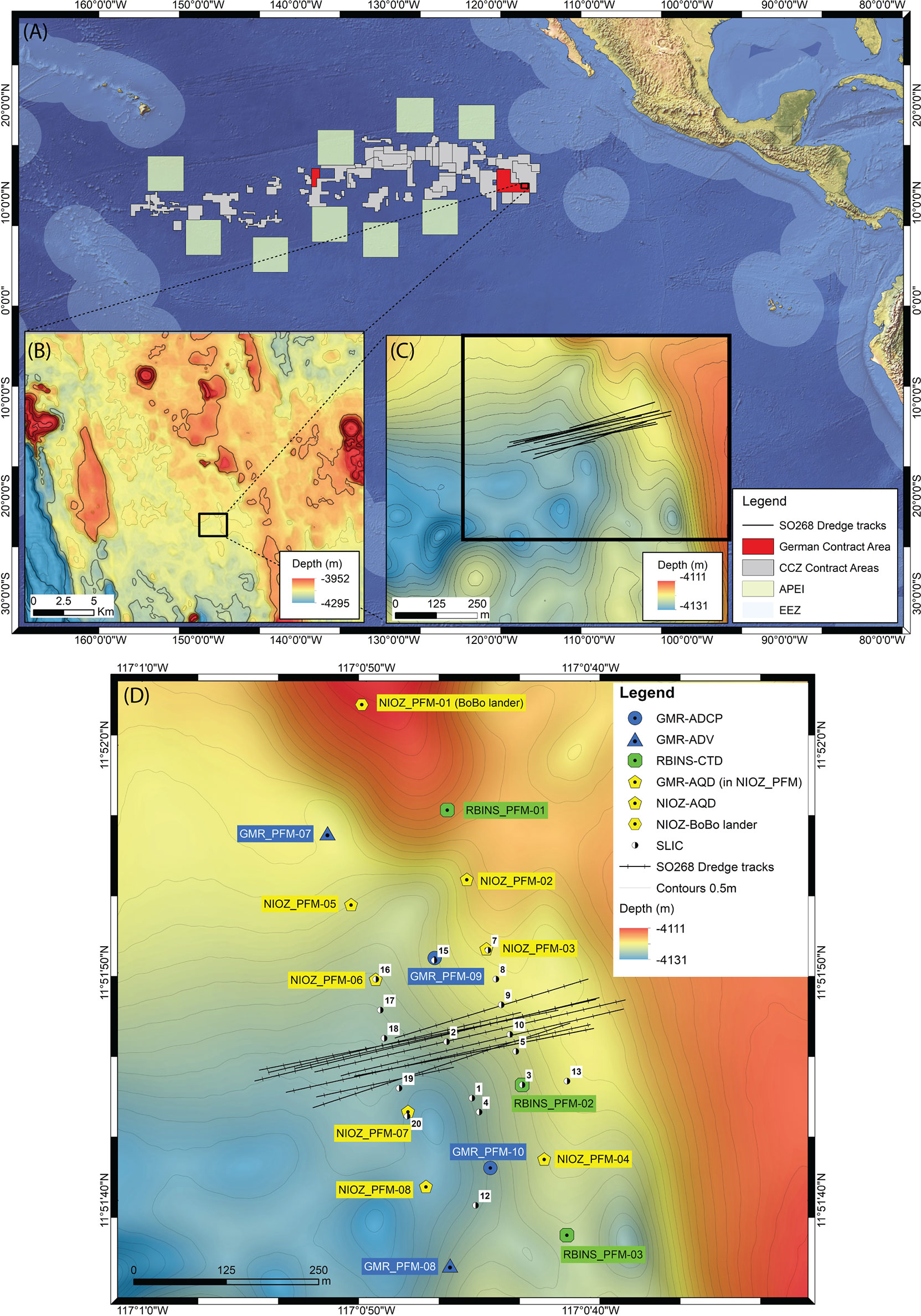
Figure 1 (A) Map showing the overall location of the CCZ with the German exploration contract areas marked in red. The area of the dredge experiment is shown in more detail in the insets (B, C). The abbreviation APEI stands for Area of Particular Environmental Interest (source: https://isa.org.jm) and EEZ stands for Exclusive Economic Zone (source: https://www.marineregions.org). (D) Locations of the sensor platforms and SLIC boxes in relation to the dredge tracks. The trajectory of the dredge on the bottom was measured during dredging using a USBL beacon mounted to the wire 500 m ahead of the dredge. Post-dredging visual inspection using USBL-navigated OFOS and ROV video footage improved the accuracy of the observed dredge track locations. Sensor platforms of the different scientific institutes involved have been allocated different colours. Bathymetric data were gathered during RV Sonne cruises SO239 (Martínez Arbizu and Haeckel, 2015; Peukert et al., 2018) and SO268 (Gazis, 2020; Haeckel and Linke, 2021). The isobath contour interval in (B) is 100 m for the darker contours and 25 m for the shaded contours, in Figure (C, D) the isobath contour interval is 0.5 m.

The surface sediment consists of a mixture of siliceous ooze and deep-sea clay, containing small amounts of detrital carbonate and volcanic material (BGR Bundanstalt für Geowissenschaften und Rohstoffe, 2018). Surface sediments have a median grain size of 20 μm and a size distribution of <10 μm (28%), 10-63 μm (57%), and >63 μm (15%) (Gillard et al., 2019). The porosity of the top 10 cm is about 84-93% and wet bulk density amounts to 1.2 g cm^-3 (BGR Bundanstalt für Geowissenschaften und Rohstoffe, 2018). The surface of the seafloor at the dredge experiment location is covered with manganese nodules with a size range from 3 to 13.5 cm, covering about 49% of the seafloor (Schoening and Gazis, 2019a; Schoening and Gazis, 2019b).

The bottom currents are characterised by a semi-diurnal M2 tidal cycle, as well as a diurnal S1 tidal cycle (Aleynik et al., 2017). Generally, the bottom current speeds are low, with average speeds of approximately 3.5 cm s^-1 and peak values usually below 10 cm s^-1. However, during the passage of mesoscale eddies, which have their clearest expression at the ocean surface but of which the effect occasionally extends to the seafloor at >4 km depth, average current speeds increase to ~8 cm s^-1, with peak values of up to 24 cm s^-1 (Aleynik et al., 2017). Whilst background bottom currents are probably not strong enough to resuspend surface sediment most of the time, resuspension might well occur under peak bottom currents associated with these mesoscale eddies (Purkiani et al., 2020). Direct observations of sediment resuspension by eddies do not exist from the area. However, the occurrence of intermittent resuspension events was inferred from the observation that nodules covered by sediment settled from a plume around an epibenthic sledge (EBS) track in 2015 (Peukert et al., 2018) were free of sediment cover when the EBS track was revisited in 2019 during the SO268 cruise (Haeckel and Linke, 2021). With several mesoscale eddies passing annually over the area (Purkiani et al., in review), it is not unlikely that at least one eddy between 2015 and 2019 has been strong enough to remove and redistribute the sediment settled on the seafloor in 2015.

3 Methods

3.1 Monitoring Plume Dispersion and Sediment Redeposition

In this small-scale plume dispersion experiment, a 1 m wide chain dredge (Figure 2) was deployed to generate a sediment plume. The dredge was dragged over the seafloor in 11 WSW-ENE trending hauls of ~500 m length each with an average speed of 0.2 m s^-1 (Table 1). It took between 40 and 60 min to complete each haul. At the end of each haul, the dredge was lifted 250-350 m above the seafloor to bring it vertically below the ship, and then lowered back to the seafloor for the next haul. The dredging was carried out on the 11^th of April 2019 and lasted for 12.5 hours (06:30 – 19:00 UTC).

FIGURE 2

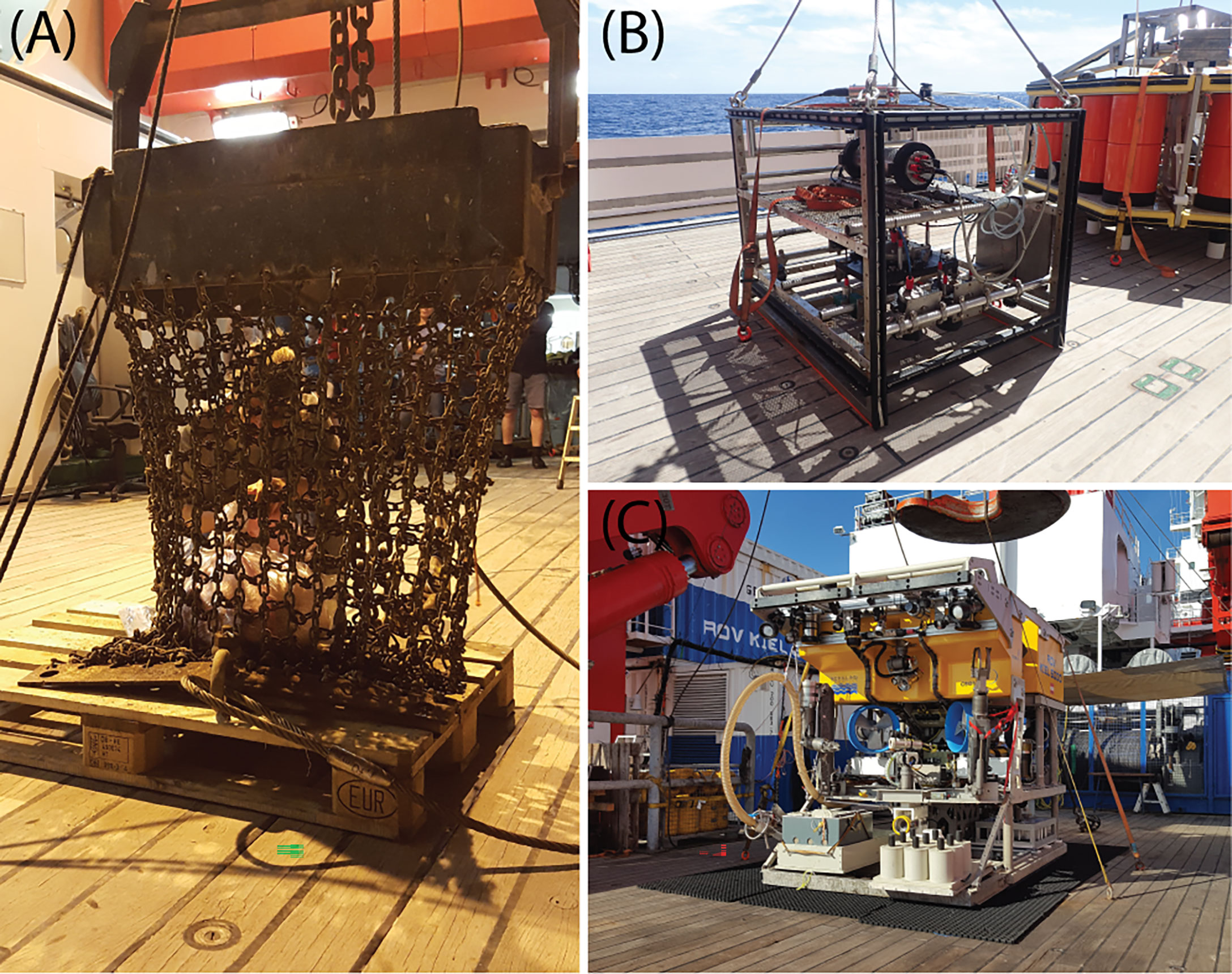
Figure 2 (A) The 1-m-wide geological chain dredge that was used to create a sediment plume in our study (photo courtesy: Henko de Stigter). (B) The Ocean Floor Observatory System (OFOS) of the RV Sonne (Photo courtesy: Yasemin Bodur). (C) Remotely Operated Vehicle (ROV) GEOMAR KIEL 6000 (Photo courtesy: Henko de Stigter).

TABLE 1

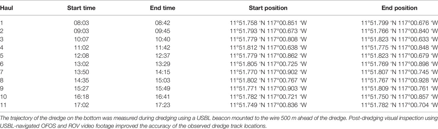
Table 1 Dredge times (UTC) and positions (longitude, latitude) of each haul on the 11^th of April 2019.

To monitor the dispersion of the generated sediment plume and mass concentration of suspended particulate matter (SPM), 15 sensor platforms were distributed around the dredge tracks prior to dredge deployment (Figure 1D). The sensor platforms were equipped with different types of optical and acoustic sensors for recording speed and direction of near-bottom currents, as well as bottom water turbidity. The platforms can be categorised into 5 different types:

1) Tripods equipped with an upward-looking Nortek Aquadopp 2 MHz current profiler recording current speed, current direction, and acoustic backscatter, and a JFE Advantech optical backscatter sensor (OBS) recording turbidity. NIOZ deployed seven of these platforms, named NIOZ_PFM-02 to -08.

2) Tripods equipped with a Nortek ADV current meter recording current speed and direction, together with a JFE Advantech OBS recording turbidity. GEOMAR deployed two of these platforms, named GMR_PFM-07 and -08.

3) Tripod frames with an upward-looking RDI Workhorse 300 kHz ADCP cardanically suspended in the frame, recording current speed, current direction, and acoustic backscatter. GEOMAR deployed two of these platforms, named GMR_PFM-09 and -10.

4) Frames holding a SeaBird 19+ CTD placed upright on the seafloor on a rectangular base plate, recording conductivity, temperature, and pressure as well as turbidity using two Seapoint OBSs recording turbidity. RBINS deployed three of these platforms, named RBINS_PFM-01 to -03.

5) A Bottom Boundary (BoBo) lander (van Weering et al., 2000) equipped with an upward-looking RDI Workhorse 300 kHz ADCP and a downward-looking RDI Workhorse 1200 kHz ADCP, recording current speed and direction and acoustic backscatter, a SeaBird 16+ CTD recording conductivity, temperature, pressure, and turbidity through a WetLabs FLNTU OBS, and a stand-alone JFE Advantech OBS recording turbidity. One BoBo lander was deployed by NIOZ, named NIOZ_PFM-01.

A summary of the sensor platform specifications, including information on measuring range, sampling intervals and deployment and recovery times is provided in Table 2.

TABLE 2

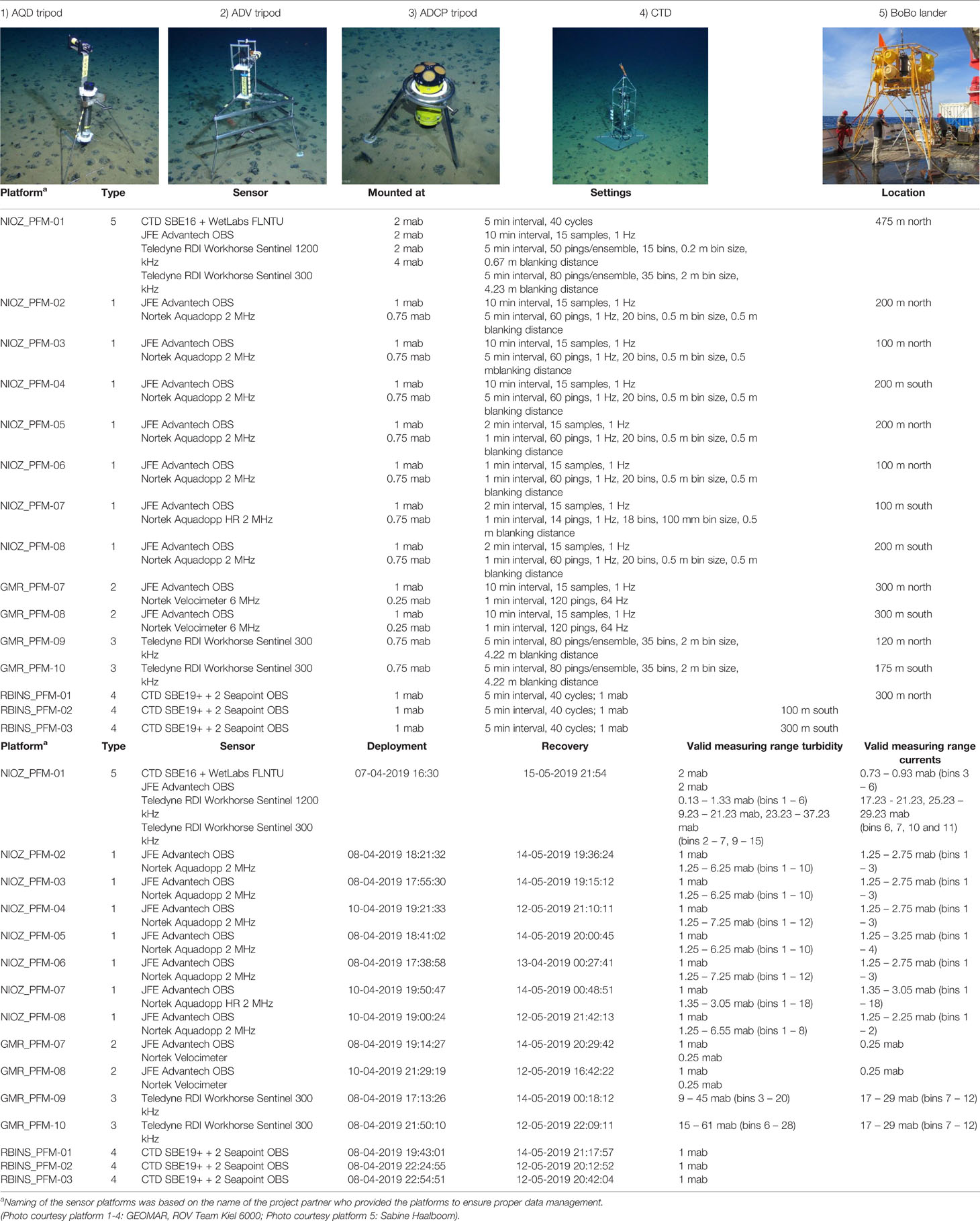
Table 2 Specifications of all sensors used in the monitoring array around the dredge experiment site.

The initial sensor layout for monitoring the plume generated by Patania II was based on a plume dispersion probability map, produced on the basis of numerical simulation using the MIT-gcm hydrodynamic model combined with a sediment transport module (for a detailed description see Purkiani et al., 2021) (Figure 3). The numerical model was driven by 10 years of wind data, affecting the oceans’ surface currents (2009-2019; Figure 3A) and throughout the open boundaries with horizontal current velocities obtained from a reanalysis of model products of HYCOM (Purkiani et al., 2021). Model results were validated with long-term current data acquired through oceanographic mooring deployments by BGR (Figure 3C). Based on the model prediction, sediment plume sensors were planned to be distributed over kilometres. For the dredge experiment, the sensor array had to be downscaled in extent to adjust to a much smaller plume generated over a shorter timeframe than anticipated for the Patania II trial (12 h vs. 4 days). The overall NNW-SSE spread of sensors as in the original layout was maintained, as this was based on the long-term prediction of current direction at the time during and after the experiment, but sensors were distributed much closer to each other and to the dredge area. Furthermore, sensors were not only placed SSE of the dredge area according to the most probable current direction, but also NNW of the dredge area to register plume dispersion in opposite direction. The different sensor platforms were distributed at distances of 100 to 475 m away from the planned dredge area (Figure 1D). Despite that the experiment described in Peukert et al. (2018) showed almost no blanketing beyond 100 m distance from the disturbance site (EBS track), the sensors were placed not closer than 100 m from the planned dredge tracks to allow some navigation inaccuracy in towing of the dredge in 4120 m water depth. The majority of the sensor platforms were distributed on two parallel lines spaced 200 m apart and perpendicular to the WSW-ENE trending dredge tracks. This distribution provided replication of the plume signal recordings on either side of the dredge tracks and enabled for a more comprehensive monitoring of the spatial distribution of mobilised sediments. Along these two parallel lines the sensor platforms were placed 100, 200 and 300 m away from the dredge area, with platforms GMR_PFM-09 and GMR_PFM-10 located in the middle of the sensor array at respectively 120 m north and 175 m south of the dredge tracks (Figure 1D). The BoBo lander (NIOZ_PFM-01) was placed 475 m north of the dredge tracks. This was because the lander was deployed free fall, making accurate positioning difficult. BoBo served as a reference for background conditions and to record the far-field plume in case the current direction would be towards the north. All other sensor platforms were deployed accurately by ROV, allowing to monitor gradients of SPM concentration at varying distances away from the dredge tracks.

FIGURE 3

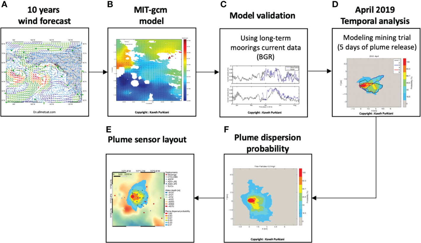
Figure 3 Development of plume dispersion probability map, used as a basis for determining the actual sensor layout for plume monitoring. (A) Gathering 10-year wind forecast. (B) Forcing data in the MIT-gcm hydrodynamic model. (C) Validation of the model using long-term mooring current data as obtained by BGR. (D) Temporal analysis of plume dispersion based on integration of a sediment transport module. (E) Plume dispersion probability map. (F) Plume sensor layout map.

Most of the sensors along the western line were set to record the dredge plume at a relatively high sampling rate that allowed high temporal resolution but limited their battery lifetime to approx. 1 week (Table 2). Sensors along the eastern line were set to record at a lower sampling rate to extend battery lifetime to 6 weeks or more. This setting sacrificed temporal resolution during the plume monitoring experiment to extend the recording timeframe of the sensors, in order to potentially record resuspension of deposited plume sediment under the influence of a mesoscale eddy that was concomitantly passing over the German exploration contract area in a westward direction at this time (Purkiani et al., in review). To increase spatial resolution two sensor platforms (NIOZ_PFM-03 and NIOZ_PFM-07) were relocated one day after dredging (12^th of April) into the dredge tracks, to monitor potential resuspension at a place where the deposited sediment thickness was expected to be highest.

Visual inspection of sediment deposition was undertaken using video cameras on the towed Ocean Floor Observations System (OFOS) and on GEOMAR’s KIEL 6000 ROV (Figure 2). Video footage of both OFOS and ROV was manually annotated during the deployments using the OFOP software package (Huetten and Greinert, 2008). Preliminary seafloor categories were “dredge track”, “faint sediment coverage (<1 mm)”, “thick sediment coverage (>1 mm)” and “no sediment coverage”. Additionally, 16 Sediment Level IndiCator (SLIC) boxes were deployed throughout the sensor array, with some only 50 m away from the dredge tracks (Figure 1D). These SLIC boxes were originally intended to collect sediment from the Patania II induced plume, and then to be photographed by the ROV or an autonomous underwater vehicle (AUV). This would provide an estimation of the thickness of the sediment drape deposited from the plume. However, since the remobilised sediment from the small-scale dredge experiment was orders of magnitude lower than what was expected from a mining plume, the SLIC boxes only provided a qualitative impression of the sediment redeposition. The SLIC boxes were photographed by the ROV immediately after their deployment and revisited 24 to 30 hours after dredging to assess sediment deposition qualitatively (Supplementary Figure 1).

3.2 Data Processing and Quality Assessment

Sensor data were averaged over the set ensemble interval either internally during the recording process (RDI Workhorse ADCP; Nortek Aquadopp profiler; WetLabs FLNTU OBS; Seapoint OBS) or externally during data evaluation (JFE Advantech OBS) (see Table 2). The quality of the turbidity data recorded by the optical sensors (JFE Advantech OBS; WetLabs FLNTU OBS; Seapoint OBS) was assessed by a feasibility check and showed no signs of spurious turbidity values or instrumental drift. Furthermore, data recorded during deployment, relocations and/or recovery of the sensor platforms was removed. The quality and reliability of the acoustic data (current speed and acoustic backscatter data) was checked for each acoustic bin of the respective ADCP. Current speed and direction data were generally discarded from bins for which the standard deviation of the u- and/or v-velocity was more than 0.050 m s^-1, as this value represents the upper limit of the background current velocities (Aleynik et al., 2017). This typically coincides with bins where the acoustic backscatter was lower than 25 counts or 40 counts for the Nortek Aquadopp and RDI Workhorse ADCP respectively, which are provided as a lower limit for good data by the manufacturers (Nortek, 2017; Deines, 1999). Table 2 specifies for each sensor which bins were regarded as valid for current speed and direction as well as backscatter intensity.

The recorded acoustic backscatter in counts for the RDI and Nortek sensors were converted to (uncalibrated) acoustic backscatter (ABS) in decibels using Eq. 1 (Lohrmann, 2001), correcting the recorded signal for loss by acoustic spreading and absorption by water (α_w):

$\begin{array}{ll}ABS\left[dB\right]=0.46\ast ABS\left[counts\right]+20\ast lo{g}_{10}\left(R\right)+2{\alpha }_{w}R+20\ast R{\displaystyle \int {\alpha }_{p}dr}& \text{(Eq. 1)}\end{array}$

where the value of 0.46 represents the count-to-decibel conversion factor (k_c = 127/(T + 237.15)) (Manik et al., 2020), with T as seawater temperature, R represents the distance from the transducer head to the middle of the measurement bin in metres, and α_w and α_p represent the absorption coefficient by water and particles, respectively. The water absorption coefficient (α_w) was determined following the Ainslie and McColm (1998) model, with temperature, depth, and salinity values of 1.5°C, 4.3 km and 34.7, respectively. This results in a water absorption coefficient of 1451.7 dB km^-1 for the 2 MHz Nortek Aquadopp profilers and coefficients of 530.2 dB km^-1 and 44.2 dB km^-1 for the 1200 kHz and 300 kHz RDI Workhorse ADCPs, respectively. In our calculation we discarded particle absorption α_p, which is unknown but considered to be negligible at the measured low concentrations of SPM.

3.3 (Inter)calibration of Turbidity Sensors

Three different types of optical backscatter sensors were used in this study (JFE Advantech, WetLabs FLNTU and Seapoint OBS). For converting the sensor outputs to SPM mass concentration (mg dry weight L^-1), it is essential to (inter)calibrate the sensors for the type of sediment present in the area. To achieve this, sensors were immersed in sediment suspensions of stepwise increasing concentration contained in a 50 L container, after which sensor response in FTU, NTU or voltage was recorded for one or two minutes. The calibration was carried out on board the research vessel in a darkened, cold room at 4°C. To avoid interference between instruments and provide sufficient sensor reading windows, each sensor was calibrated separately (Supplementary Figure 2). Stock suspensions had been prepared prior to the cruise from the top 10 cm sediment layer of a box corer sample taken in the German exploration contract area by BGR (sample KG-172, research cruise SO262) mixed with artificial seawater. By adding doses of stock suspension to the 50 L calibration container filled with unfiltered bottom water collected from the test site, the SPM mass concentration was increased in seven steps from 0 mg L^-1 to 1640 mg L^-1. This SPM range was chosen to cover all sensor-specific detection limits and to include one additional step to assure complete detection range coverage. The outlet of a pump system (3000 L h^-1) was placed at 45° onto the container bottom to assure complete mixing during calibration. The sensors recorded the turbidity at their highest sampling rate (1 to 10 seconds). To determine the SPM mass concentration of the successive calibration suspensions, triplicate samples (36.12 ± 0.57 mL) were taken from the suspension after each calibration step. After the cruise, the complete volume of these sub-samples was filtered through a dried, pre-weighed 25 mm diameter, 0.2 μm cellulose acetate filter (Sartorius). After each filtration, the filter was carefully rinsed twice with Milli-Q water to remove remaining salt and dried before it was weighed to obtain the sediment weight. The drying of the clean filter or the filtered sample occurred in an oven (Heraeus, Thermo Scientific) at 60°C for 48 hours. The turbidity values recorded by the sensors showed a good linear relationship with the corresponding SPM mass concentrations for all the OBSs, with an R² of ~0.98 (Figure 4A for the OBSs used on platforms NIOZ_PFM-08 and RBINS_PFM-03). The sensor-specific linear relation was used for the conversion of sensor output data to SPM mass concentration.

FIGURE 4

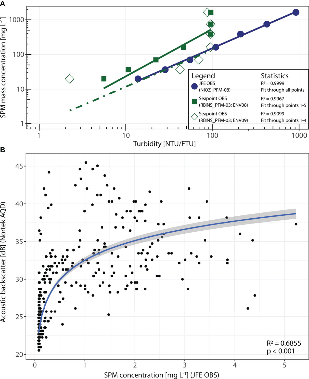
Figure 4 (A) Correlation between recorded turbidity of several optical backscatter sensors (OBSs) as measured during onboard calibration and SPM mass concentration. Results are shown for the JFE Advantech OBS NIOZ_ENV14 as used on platform NIOZ_PFM-08 (blue) and the Seapoint OBS RBINS_ENV08 (SP1; green solid squares) and Seapoint OBS RBINS_ENV09 (SP2; green open squares), used on sensor platform RBINS_PFM-03. The linear regressions are used for the conversion of the recorded turbidity signal into SPM mass concentration. Note that for the Seapoint OBSs the regression line is only fitted to the first 4 or 5 points, as the other higher calibration steps were beyond the saturation level of these OBSs, resulting in a constant response (saturation) of these sensors above 100 NTU. (B) Correlation between SPM mass concentration as recorded at sensor platform NIOZ_PFM-08 (200 m south of the dredge tracks) by a JFE Advantech OBS (x-axis) and converted acoustic backscatter in dB as recorded by the Nortek Aquadopp profiler (y-axis) at the same site on the 11^th of April.

The acoustic backscatter recorded by the acoustic sensors could not be directly calibrated on board in a similar manner as done for the OBSs, due to the relatively large minimum measurement range of the acoustic sensors. Following a practice described in other studies (e.g., Fettweis et al., 2019; Haalboom et al., 2021), the Nortek Aquadopp sensors were calibrated in situ by reference to the SPM mass concentration derived from a calibrated OBS placed close to the first valid measurement bin of the Aquadopp. This is exemplarily shown for sensors of platform NIOZ_PFM-08. The lowermost bin of the Nortek Aquadopp was at 1.25 metres above bed (mab), while the JFE OBS was recording at 1 mab. As shown in Figure 7 the recorded turbidity patterns show similarities in terms of amplitude and timing on the 11^th of April. The cross-comparison of these data points (SPM mass concentration on a linear scale, acoustic backscatter as decibels; Figure 4B) revealed a significant (p < 0.001), though not particularly strong (R² = 0.6855) log₁₀ relation between these two time series. Applying this relationship to convert the acoustic backscatter levels to SPM mass concentration results overall in a much higher estimate of the SPM mass concentration compared to what was inferred from the OBSs. Due to these large differences and uncertainties about what exactly caused them, we refrain from using the acoustic backscatter results in any quantitative analysis. Even so, the acoustic backscatter data (converted to dB) provide valuable qualitative insight in the occurrence of sediment plumes in time and space, in particular regarding the vertical extent of these plumes above the seabed.

3.4 Different Particle Size Sensitivity of Turbidity Sensors

Optical backscatter sensors are known to be more sensitive to fine-grained particles, whilst their sensitivity decreases with increasing particle size (e.g., Downing, 2006). For acoustic sensors, the sensitivity depends on the particle size and other particle parameters (e.g., density, shape; Fettweis et al., 2019 and references therein) as well as on the operating frequency of the acoustic device (e.g., Wilson and Hay, 2015). However, to gain a basic comparison of the particle size sensitivity of the used acoustic sensors, the simple approximation from Lohrmann (2001) can be used. The model states that the sensor response is at its maximum when ka = 1, with k being the acoustic wave number given as $k=\frac{2\pi f}{c}$, with f being the operating frequency and c the speed of sound, and a the particle radius. For particle radii of ka < 1 the acoustic sensitivity decreases proportionally to the particle radius to the fourth power, and for particle radii of ka > 1 the acoustic sensitivity is predicted to behave inversely proportional to the particle radius. Applying this to the acoustic sensors used in our plume monitoring experiment, operating at 300 kHz, 1200 kHz and 2000 kHz (Table 2), these sensors have maximum sensitivity for particles of, respectively, 1618 μm, 404 μm and 242 μm diameter, taking the speed of sound as in the study area at 4 km depth (1525 m s^-1). Already at a tenth of this diameter (162 μm, 40 μm and 24 μm respectively), the sensitivity of these sensors decreases by approximately -40 dB (factor 10.000).

3.5 Water Column SPM Mass Concentration

During the SO268 cruise, five CTD casts were performed in the dredge area to determine the SPM mass concentration in the water column. During each of the CTD casts, a bottom water sample (~4119 m water depth) was taken in duplicate using 11 L Niskin bottles. From the Niskin bottles, subsamples of either 4.5 L or 9 L were drawn (Table 3) and filtered on board over 47 mm diameter, 0.4 μm pre-weighed Millipore polycarbonate filters. The filters were rinsed with Milli-Q to remove salt and stored at -20°C until further analysis. In the laboratory at NIOZ, the thawed filters were rinsed again with Milli-Q to remove still remaining salt, and subsequently freeze-dried and weighed to determine the weight of SPM per volume of filtered seawater.

TABLE 3

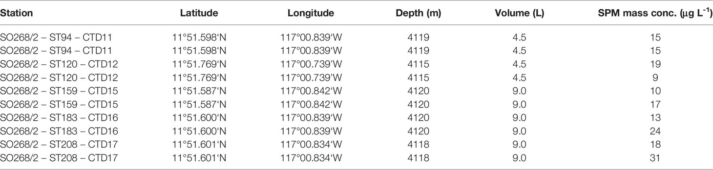
Table 3 SPM mass concentration obtained from bottom water samples at five CTD stations during cruise SO268.

4 Results

4.1 Bottom Water Background Characteristics

Based on CTD data, the bottom water in the study area is characterised by a temperature of 1.5°C, a salinity of 34.7, a density (σ-θ) of 27.8 kg m^-3, and SPM mass concentrations of 0.02 mg L^-1, as inferred from the JFE Advantech OBS (Supplementary Figure 3). Such low concentrations correspond to values obtained from the Niskin water samples collected in undisturbed, clear bottom water, which showed average SPM mass concentrations of 0.017 ± 0.006 mg L^-1. Low turbidity values were recorded throughout the water column below thermocline depth, and no increase in turbidity towards the seafloor that would indicate the presence of a bottom nepheloid layer was detected. Throughout the 6 weeks of monitoring, mean current speeds close to the seafloor (< 20 mab) were about 4 cm s^-1, predominantly in southeast direction, with alternations towards the north. Higher in the water column, between 20 and 30 mab, mean current speeds increased to 6 cm s^-1, still having the same dominant current direction. Spectral analysis showed that the current regime is dominated by the semidiurnal and diurnal tidal harmonic components M2 and K1 (Supplement Figure 4).

4.2 Visual Observations of the Dredge’s Impact on the Seafloor

Based on the ROV and OFOS images (Figure 5) it could be confirmed that the dredge did not remove or stir up the sediment equally along its predefined tracks. The dredge was effectively dragged over the seafloor along some parts of the transects, with much of the sediment being pushed aside as a cohesive mass and thus not fully put into suspension. Along other parts of the dredge tracks, we found that the dredge had bounced over the seafloor and had hardly touched the seafloor at all, or only scratched the surface. Furthermore, lumps of cohesive sediment were observed to be scattered outside of the dredge tracks, which most likely were dropped when the dredge was hauled up at the end of each track and moved into position to start the next track.

FIGURE 5

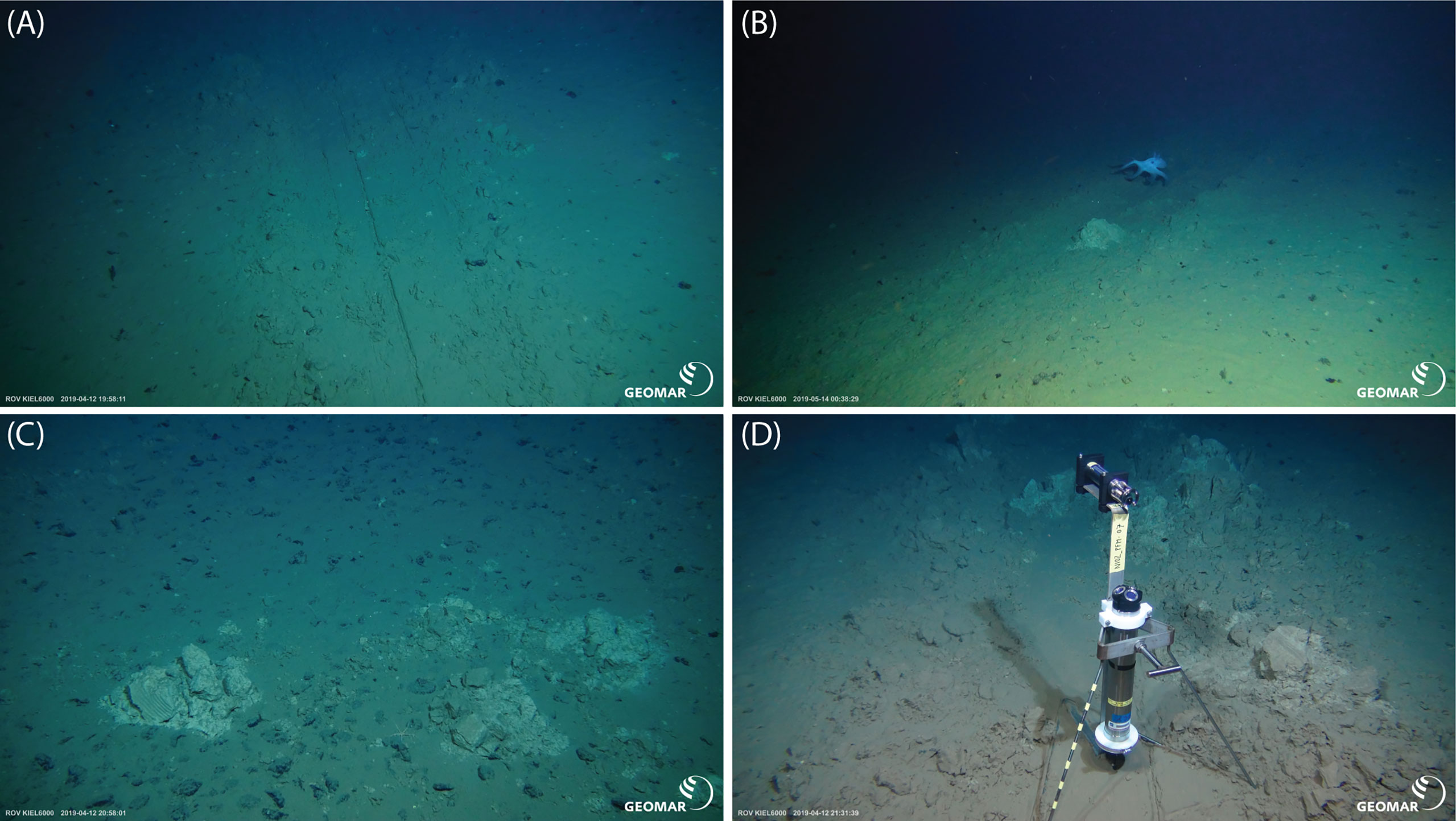
Figure 5 (A) The 1-m-wide dredge track, with sediment pushed to the side. On both sides of the dredge track the blanketing of the polymetallic nodules is observed. (B) Variability in depth of the dredge mark. In the foreground the 1-m-wide dredge only swept over the sediment surface but further down the dredge mark deepens and more sediment was pushed sideways. The photo also shows a churned-up sediment lump in the middle of the track and an octopus behind. (C) Sediment lumps found outside of the dredge tracks, presumably fallen from the dredge as it was hoisted up from the seafloor. (D) Photo showing NIOZ_PFM07 after it was repositioned into the dredge track on the 12^th of April. More photos are found in the SO268 cruise report (Haeckel and Linke, 2021). (Photo courtesy: GEOMAR, ROV Team Kiel 6000).

4.3 Sensor Data on Sediment Plume Dispersion

During the dredging (11^th of April 06:30 – 19:00 UTC), the recorded current patterns were generally consistent between all sensors (Figure 6). At the start of the dredging (between 06:30 and 11:00 UTC), the currents were directed towards the southeast, with average current speeds of 2 to 3 cm s^-1 (Figure 6). From 11:00 UTC onwards until the end of the dredging at 19:00 UTC, the currents turned clockwise towards the south, with maximum current speeds reaching 7 cm s^-1. This pattern of initial flow towards the southeast turning more to the southwest at a later stage is depicted in progressive vector diagrams showing cumulative displacement (Supplementary Figure 5), where differences between the platforms become apparent from the diverging trajectories.

FIGURE 6

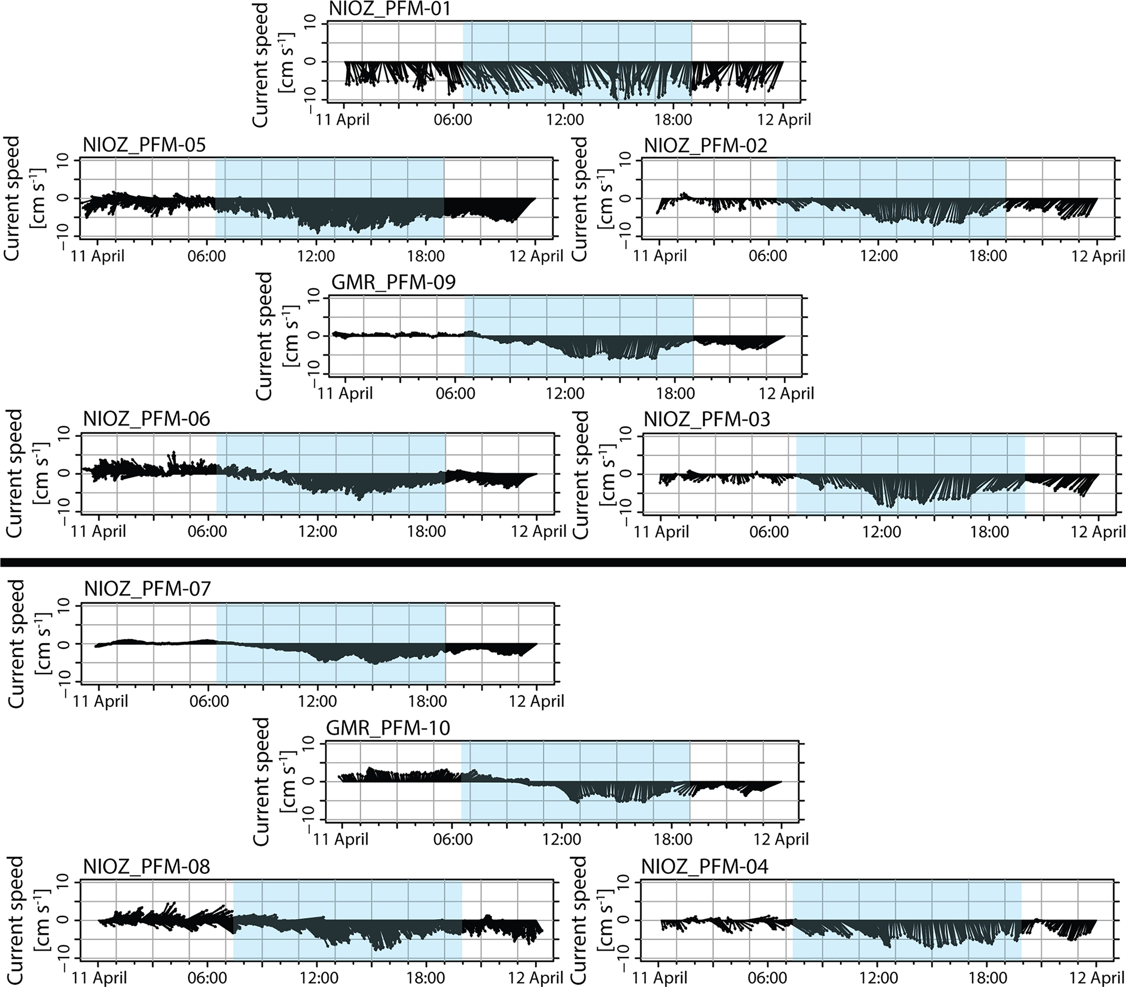
Figure 6 Time series of current speed and direction recorded on the 11^th of April by the Nortek Aquadopp profilers (bin 1 at 1.25 mab, NIOZ_PFM-02 to -08) and the RDI Workhorse ADCPs (bin 7 at 19 mab, GMR_PFM-09 and -10, and bin 3 at 0.7 mab, NIOZ_PFM-01) located north and south of the dredge tracks. The blue overlay indicates the time interval during which the dredging took place. The arrangement of the time series graphs corresponds with the geographical arrangement of the sensor platforms north and south of the dredge tracks (black line through the centre).

In agreement with the observed current directions, the time series of SPM mass concentration recorded at the different sensor platforms reflect a southward entrainment of the sediment plume. Both during and after the dredging, the sensors north of the dredge tracks did not record increased SPM mass concentrations but remained at the background SPM mass concentration of 0.02 mg L^-1 (Figure 7). In contrast, the sensors south of the dredge tracks recorded repeated increases in SPM mass concentration well above background level. The recorded maximum SPM mass concentrations decreased with increasing distance from the dredge area. At platforms NIOZ_PFM-07 and RBINS_PFM-02, both 100 m south of the dredge tracks, 5 intervals of enhanced SPM mass concentrations of ~3 mg L^-1, with maxima going up to 11 mg L^-1, were recorded between 09:00 and 18:00 UTC, and between 10:00 and 18:00 UTC, respectively (Figure 7). At sensor platforms NIOZ_PFM-08 and NIOZ_PFM-04, located 200 m south of the dredge tracks, the passing plumes were recorded between 10:00 and 19:30 UTC, and between 10:00 and 14:00 UTC, respectively, with SPM mass concentrations of ~2 mg L^-1. At platforms GMR_PFM-08 and RBINS_PFM-03, both located 300 m south of the dredge area, the plumes were recorded from 11:30 to 20:00 UTC, and from 11:00 to 14:30 UTC, respectively, with lower SPM mass concentrations of ~1 mg L^-1, still clearly exceeding the background SPM concentration.

FIGURE 7

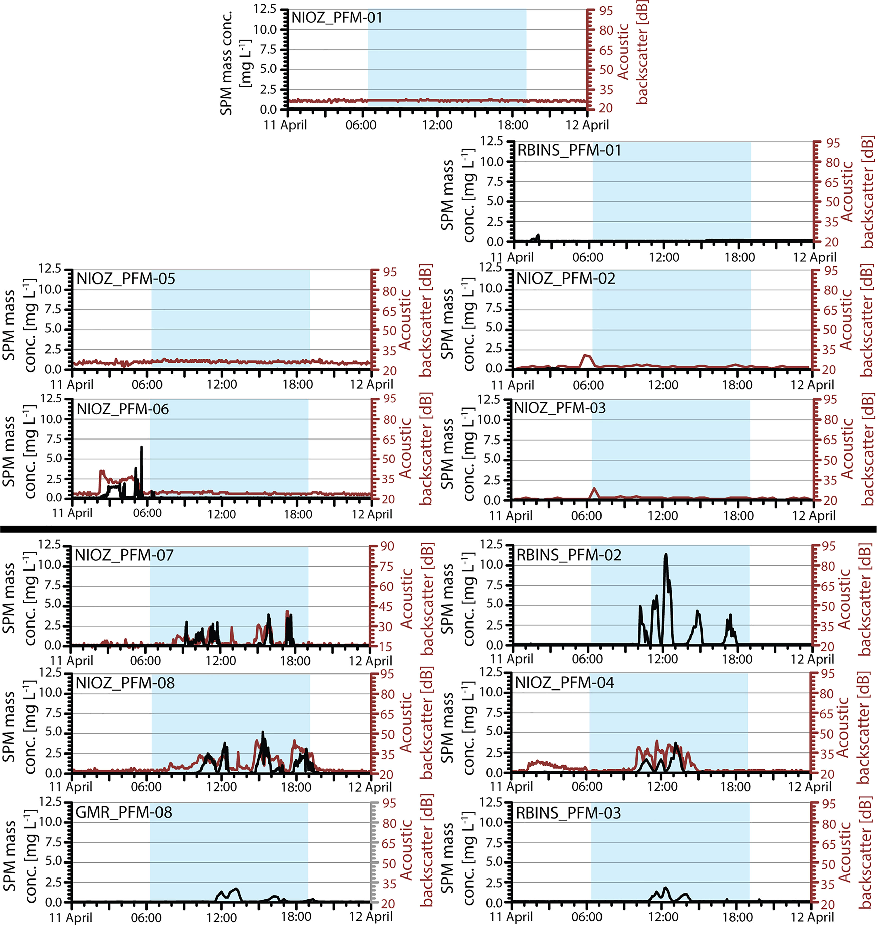
Figure 7 Time series of SPM mass concentration as inferred from OBS measurements at 1 mab (black) and acoustic backscatter at 1.25 mab (red) recorded on the 11^th of April. The blue overlay indicates the time interval during which the dredging took place. The arrangement of the time series graphs corresponds with the geographical arrangement of the sensor platforms north and south of the dredge tracks (black line through the centre). It should be noted that in the representation of relative turbidity using a decibel scale, variation in the low concentration range appears disproportionally enhanced compared to variation in the high concentration range. The observed increase in recorded turbidity by both the optical and acoustic sensors of platform NIOZ_PFM-06 in the hours before the dredging took place, can be attributed to the sediment plume produced by lift-off of the elevator that was used for transferring sensor platforms from the ship to the seafloor. The elevator was located 80 m NE of the platform, while current at the moment of lift-off was in southwesterly direction.

The drift speed of the plumes away from the dredge area, as inferred from the arrival times of the plume at the different sensor platforms, is in good agreement with the current speeds recorded close to the seafloor at that time. For example, the maximum recorded SPM mass concentration of the first plume, indicating the main body of the first plume, was recorded at 10:30, 11:00 and 12:00 UTC, at sensor platforms NIOZ_PFM-07 (100 m), NIOZ_PFM-08 (200 m) and GMR_PFM-08 (300 m), respectively. This gives current speeds ranging from 2.8 to 5.6 cm s^-1, in line with the currents measured between 10:30 and 12:00 UTC by NIOZ_PFM-07 (ranging from 2.8 cm s^-1 to 5.3 cm s^-1).

The acoustic backscatter recorded from the lowermost measurement bin of the Nortek Aquadopp profilers at platforms NIOZ_PFM-07, NIOZ_PFM-08 and NIOZ_PFM-04 was compared to the OBS data from the same platforms. As shown in Figure 7, the acoustic backscatter recorded at those platforms displayed several sharp increases, and subsequent decreases to background level, predominantly in parallel with SPM mass concentration changes recorded by the OBSs. However, we observe some differences between the acoustic and optical data in the arrival time, peak value, and end of successive plume events. Typically, the acoustic sensors detected the initial increase in turbidity marking the arrival of the plume considerably earlier than the optical sensor on the same platform, in some cases up to one hour earlier. The maximum turbidity within successive plume events was usually also recorded first by the acoustic sensor, by up to an hour earlier than the corresponding OBS sensor. The return to background turbidity levels, however, was usually recorded at the same time by both sensor types. This mismatch between the simultaneously measured acoustic and optical backscatter is also evident in the broad scatter seen in Figure 4B.

Inspection of the entire turbidity profile obtained from the Nortek Aquadopp profilers allows estimation of the height of the plume. The densest part of the plume stayed within 2 m above the seafloor, but occasionally rose to 6 mab, as shown in Figure 8 for NIOZ_PFM-08 and NIOZ_PFM-04 that were located 300 m south of the dredge tracks. The 300 kHz ADCP at platform GMR_PFM-10, which due to its lower frequency has a larger detection range, was installed to predominantly record coarser grained (aggregated) particles. Unfortunately, this sensor also has a larger blanking distance and only started recording at 5 mab. Furthermore, the lowermost bins did not provide trustworthy data so that good data could only be obtained from 19 mab upwards. Thus, the RDI 300 kHz ADCPs missed the lower part of the plume, but the 300 kHz ADCP sensor at platform GMR_PFM-10 (Figure 8) did show a peculiar backscatter pattern up to 60 mab close to the end of the dredging at 18:00 UTC.

FIGURE 8

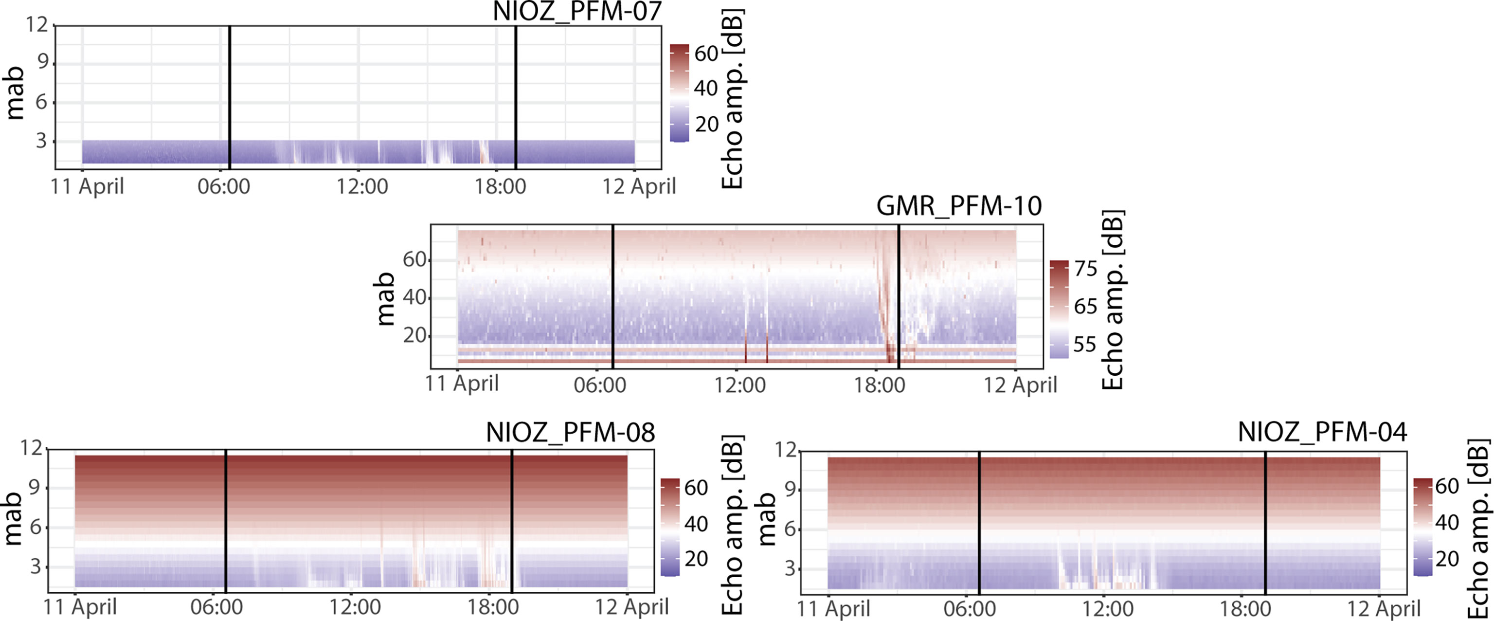
Figure 8 Time series of acoustic backscatter (converted to dB) in the lower metres or tens of metres above the seabed (mab) recorded with Nortek Aquadopp profilers (on NIOZ_PFM-04, -07 and -08) and the RDI Workhorse ADCP (on GMR_PFM-10) in the southern part of the sensor array, showing the vertical extent of the sediment plume and particle swarms above the seabed. The two black lines in the figures represent the start and the end time of the dredging. The arrangement of the time series graphs corresponds with the geographical arrangement of the sensor platforms. Note the different scale of the vertical axis for platform GMR_PFM-10. The range-dependent gradual increase in background echo amplitude level is caused by acoustic loss corrections for spreading and absorption, which amplify the raw signal with increasing distance from the transducer (Eq.1). Since the acoustic absorption is frequency dependent, this increase is more pronounced for NIOZ_PFM-04, -07, and -08 (Nortek Aquadopp with 2 MHz), compared to GMR_PFM-10 (RDI ADCP with 300 kHz).

During the weeks after the dredging was carried out (11^th April to 13^th May), we observed variable current speeds and directions, as shown exemplarily for sensor platform NIOZ_PFM-04 in Figure 9 (and for all sensor platforms in Supplementary Figure 6). Currents were predominantly directed southward, occasionally alternating towards the north. After the plumes had passed, we occasionally recorded enhanced SPM mass concentrations at some of the sensor platforms (e.g., NIOZ_PFM-04; Figure 9; Supplementary Figure 7). These events can be linked to our own sampling and monitoring activities at or close to the seafloor in the near vicinity of these sensor platforms.

FIGURE 9

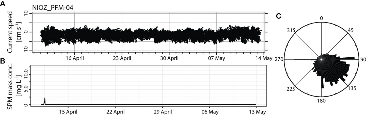
Figure 9 Longer-term variability of current speed and direction and SPM concentration at sensor platform NIOZ_PFM-04, recorded between the 11^th of April and the 13^th of May 2019, 200 m south of the dredge tracks. (A) Current speed and direction, showing predominant southeast current direction, alternating with northerly direction. (B) Recorded SPM mass concentrations during the entire deployment period. (C) Rose diagram display of the recorded current directions.

4.4 Visual Observations of Sediment Deposition From the Plume

OFOS and ROV imagery showed a drape of up to a few mm of resettled sediment (Figure 10). Observations of SLIC boxes by ROV confirmed this observation (Figure 11 and Supplementary Figure 1). These sediment drapes were only found in close proximity to the dredge tracks, and were just sufficient to cover the nodules, but not completely bury them (Figure 10C). Furthermore, we saw more resettled material in SLIC boxes 02, 05, 10 and 19 (in between or close to the dredge tracks; Figure 11 and Supplementary Figure 1). The thickness of the drape rapidly diminished in a southward direction, as shown by still images taken from SLIC boxes 01, 03, 04 and 20 (Figure 11 and Supplementary Figure 1), as well as in OFOS imagery (Figure 10B). No sediment cover related to the dredge experiment was visually discernible at distances of 100 m or more south of the dredge tracks (Figures 10A and 11). North of the dredge tracks, a faint coverage was only found in SLIC boxes 16 and 18, whereas the other SLIC boxes did not show any coverage (Figure 11).

FIGURE 10

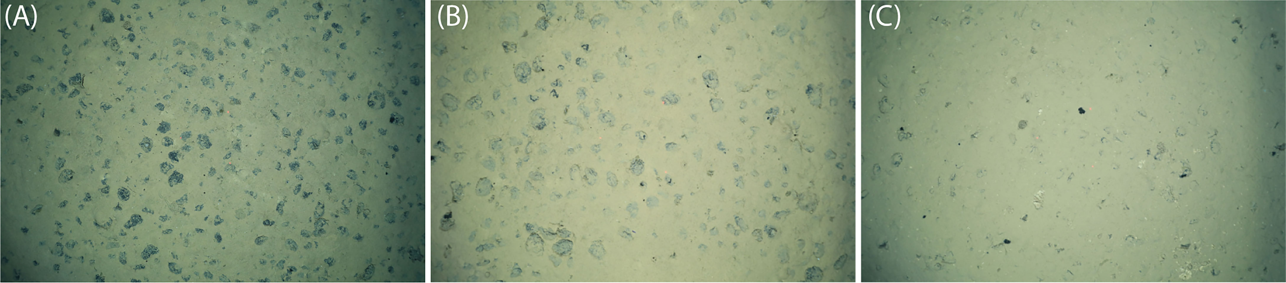
Figure 10 Still images acquired during seafloor imagery surveys using the OFOS. (A) No sediment coverage. (B) Faint sediment coverage. (C) Thick sediment coverage. Data availability: Purser et al. (2021).

FIGURE 11

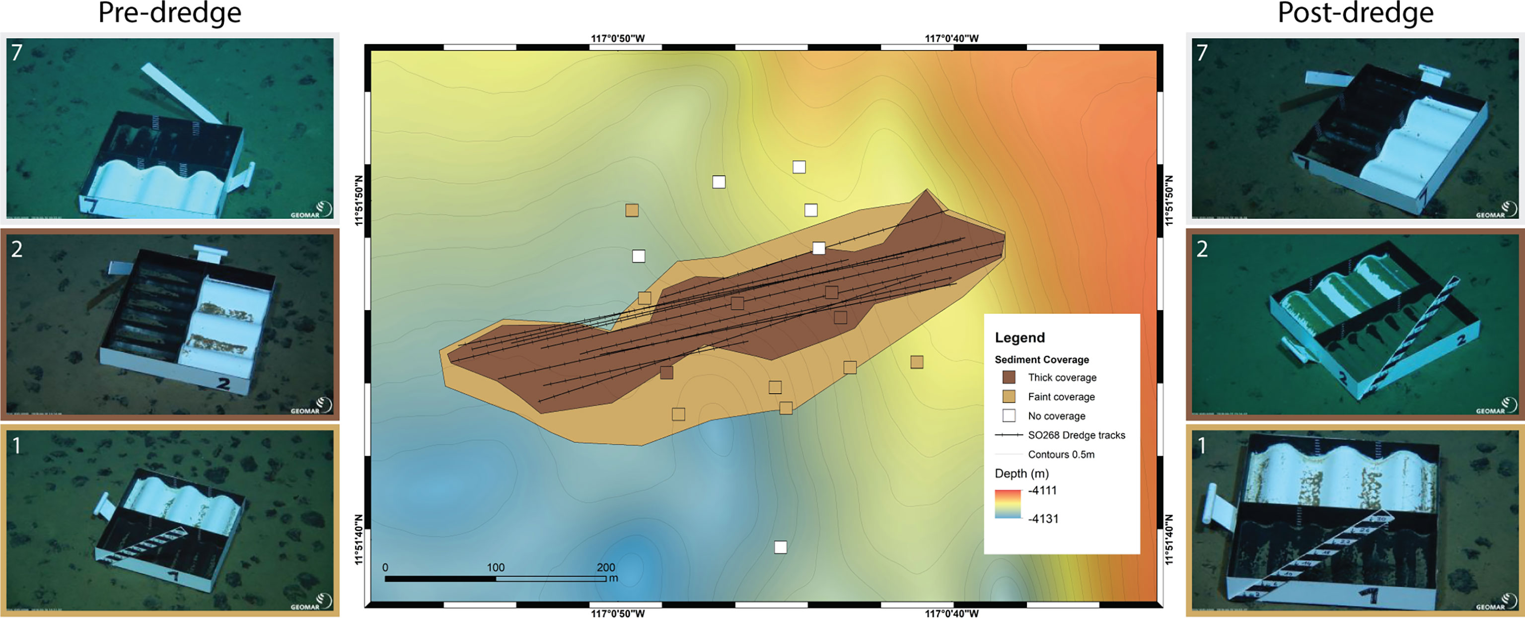
Figure 11 Map showing the visually assessed sediment coverage of the nodules, distinguishing “no coverage” (white/no colour), “faint coverage” (light brown) and “thick coverage” (dark brown) (Schoening et al., submitted). The isobath contour interval is 0.5 m. Pre- and post-dredge photos (left and right) of three SLIC boxes illustrate different amounts of sediment accumulation: no coverage (box 7, top), thick coverage (box 2, middle), and faint coverage (box 1, bottom). From these images it is clear that sediment has resettled in the troughs of the SLIC boxes, but especially in case of SLIC box 2, also forms a drape on the crests. These SLIC boxes, designed by GEOMAR, consist of two 25x50 cm sections of corrugated iron painted white and black, contained in a 50x50x8 cm iron frame. An oblique measuring stick was mounted on one side of each box. (Photo courtesy: GEOMAR, ROV Team Kiel 6000).

4.5 Virtual 4D Data Visualisation

We compiled all gathered data for visualisation in 4D using the web-based Digital Earth Viewer tool (Buck et al., 2021). A freely accessible example can be found here: https://digitalearthviewer-plume.geomar.de. This tool allows easy navigation through time and space, and an eye-catching visualisation of the dispersion of the sediment plume of the dredge experiment described here.

5 Discussion

Our monitoring array has provided an unprecedented insight into the spatial and temporal dispersion of anthropogenic sediment plumes in the abyssal ocean. Compared to impact experiments that were carried out in the past (e.g., Lavelle et al., 1982; Peukert et al., 2018; Spearman et al., 2020; Baeye et al., 2022), we placed many more sensors close to each other at well-defined locations in a large spatial array around the disturbance area. We were able to clearly detect the dispersion of the generated plume up to at least 300 m from the disturbance site. Using visual inspection, we observed sediment deposition up to 100 m away from the source. The combination of methodologies that inspect both plume sediment in suspension and plume sediment deposition is important, as both represent environmental pressures impacting the deep-sea ecosystem surrounding disturbed or mining sites (Jones et al., 2017; Washburn et al., 2019). In the following we will discuss the observed plume dispersion and sediment deposition as well as the strengths and weaknesses of our monitoring setup. We conclude with thoughts and recommendations on how to improve monitoring approaches for future larger-scale, deep-sea mining trials.

5.1 Sediment Mobilisation and Dispersion of the Plume

Our data show that the plume produced by the dredge experiment initially dispersed south of the dredge tracks, as also predicted using modelled plume dispersion probability analysis undertaken for the time of the experiment (Figure 3E). The sensor data show that the dredge activities of 11 hauls in total were neither recorded by the sensors as 11 discrete plume events, nor as a continuous plume of varying intensity. The irregular series of separate plume events, separated by shorter or longer intervals when turbidity dropped back to background values, suggests that plumes produced by some of the dredge hauls have merged, whereas some of the hauls may not have produced significant plumes. During the initial hours of dredging, the near-bottom current had an easterly component, due to which the initial plumes may have bypassed the southern sensor platforms. From the collected imagery, showing discontinuous dredge hauls of variable depth (Figure 5), it appears that the dredge did not scrape the seafloor evenly, but rather moved in a bouncing manner, at times flying over the seafloor, and at times digging more than 10 cm deep into the seafloor. In part, this could be due to a blocking of the dredge mouth with the very sticky deep-sea sediment, preventing further pick-up of nodules and sediment. This has certainly affected the amount of sediment that went into suspension, as was also observed during a small-scale disturbance experiment by Becker et al. (2001), who found that 80% of the sediment mobilised by a propeller-generated water jet remained on the seafloor. Based specifically on the field data of our study, Purkiani et al. (2021) deduced by numerical modelling that only approximately 4% of the sediment mobilised by the dredge was actually brought into suspension and reached the southern sensor platforms. Another 25% of the mobilised sediment was deposited at short distance from the track, leaving about 70% of the mobilised sediment in the dredge tracks as cohesive sediment that was only pushed aside.

Both the optical and the acoustic sensors on the seafloor detected a sequence of plume events caused by the dredging activities. However, the patterns of recorded turbidity differ between these two sensor types, even though the sensors were placed less than half a metre apart on the same platform and measured the turbidity simultaneously (Figure 7). It should be noted that initial minor increases in acoustic backscatter, marking the arrival of the plume and preceding the increase in optical backscatter, may have been disproportionately emphasised by being presented in a decibel scale. However, differences in the response of optical and acoustic sensors have been observed previously (e.g., Haalboom et al., 2021) and might be related to the differing sensitivity of optical and acoustic sensors to varying particle sizes of suspended material. We found that OBSs are most sensitive to fine-grained particles, while the acoustic sensors, depending on their operating frequency, tend towards higher sensitivity for coarser particles (Section 3.4).

Given that the median particle size in the local seafloor surface sediment is around 20 μm (Gillard et al., 2019), non-aggregated suspended sediment particles would be close to or below the wavelength limit of the Nortek Aquadopp profilers operating at 2 MHz, and even more so for the 1200 kHz and 300 kHz ADCPs. Despite this, the acoustic profilers detected clear plume signals, indicating that the plume carried sufficiently large particles to cause measurable backscatter. The sediment plume certainly contained primary sediment particles at the coarse end of the particle size spectrum but very likely also aggregated fine-grained sediment. Recent laboratory experiments by Gillard et al. (2019) have shown that under typical deep-sea flow conditions, aggregation of CCZ sediment particles occurs rapidly. Particle aggregation, producing larger-sized particles at the cost of smaller-sized particles, results in an increased intensity in the acoustic backscatter but a decrease in optical backscatter. Settling of larger particles would result in a decrease in acoustic backscatter, whilst there might be no change in optical backscatter. Aggregation occurring in the plumes as they drifted southwards may thus account for differences in intensity with which the plume was recorded by optical and acoustic sensors.

The differences in arrival times of plume events as registered by optical and acoustic sensors are, however, not explained by differences in aggregation state of the suspended particles in the plume. Fine-grained primary particles and coarser-grained aggregates are both passively transported with the currents and thus have the same horizontal velocity. Different clock times or sampling rates of the sensors can be excluded, as all sensors were programmed with the same UTC time and sampling rate and observed drift in clock times amounted to less than 50 seconds over the entire 6 weeks of the deployments. In addition, optical and acoustic sensors recorded some of the plume events almost simultaneously.

One possible explanation might be that the larger particles detected acoustically before the sediment plume was detected optically represent nektobenthos like amphipods, swarming ahead of the advancing sediment plume, but we do not know of any visual observations reported in the literature that might confirm this hypothesis. Alternatively, the acoustic sensors could have recorded a rain of sediment lumps falling out of the sediment-laden dredge as it was lifted from the seafloor at the end of each haul. Video imagery revealed many lumps of cohesive sediment scattered closely around the dredge tracks (Figure 5), but smaller parts may have been carried further away by the currents. Released at several tens of metres above the seafloor, where current speed is higher than at the seafloor, small bits of cohesive sediment raining out from the dredge may have reached the sensor platforms earlier than the plume moving southwards close to the seafloor. In this light, the peculiar reflection noted in the backscatter profile recorded by the 300 kHz ADCP on GMR_PFM-10 shortly after 18:00 UTC might also be explained in this way. In the acoustic backscatter profile recorded by the 2 MHz Aquadopp profilers at NIOZ_PFM-07, located at 135 m from GMR_PFM-10 but 50 m closer to the dredge tracks, a relatively intense vertical reflection was also observed just before 18:00 UTC.

While the hypotheses above try to explain what may be merely a side-effect of our dredge experiment, they highlight an important advantage of using acoustic profilers over optical sensors for recording turbidity. While optical sensors produce point measurements of turbidity, the acoustic sensors allow monitoring turbidity over a distance of metres to tens of metres away from the sensor head. Upward-looking acoustic profilers detect the vertical extent of the plumes. With a caveat that some of the backscatter signals may in fact represent showers of sediment falling out of the dredge, we postulate that the sediment plumes 300 m south of the dredge tracks extended 2-6 m above the seafloor (Figure 8). This is higher than the 0.96 to 1.6 m inferred by Peukert et al. (2018) for a plume produced with an epibenthic sledge (EBS) in the same study area, or the 1.5 to 2 m height of an EBS plume reported by Greinert (2015) in the Peru Basin. But these previous estimates were based on observations made at short distances of maximum 50 m from the plume source, where the plume had little time to extend vertically into the water column by turbulent mixing, while our monitoring setup spread over a distance of 300 m.

Our time series of turbidity extend until 13^th May, covering a period of one month after the dredging was performed (Figure 9). Data from this period do not show any signals of enhanced turbidity which cannot be explained by nearby ROV operations or bottom sampling gear. We have not recorded additional signals of plume dispersion even when the near-bottom current turned to a northerly direction in the day following dredging. We assume that the plume had already largely settled out at this stage and had been diluted with ambient water and was no longer detectable by the sensors, or that tails of the plumes may have bypassed the area where our sensors were positioned. By exponential extrapolation of the decrease in observed peak SPM mass concentrations with increasing distance from the dredge tracks, we estimate that the plume concentration dropped below the detection limit of our sensors within a distance of one kilometre from the source. With an average current speed of 4 cm s^-1 this corresponds to a transit time of less than 7 hours.

From the lack of any natural increase in turbidity in the weeks after the dredging, and the lack of a notable increase in near-bed current velocity, it can be inferred that the mesoscale eddy which was observed passing over our study area either had not reached the seafloor within the time interval that our sensors were deployed, or that it did not affect the deep water column and seafloor. Observed near-bottom current speeds in the CCZ generally do not exceed the critical threshold of 15 cm s^-1 required for resuspension of unconsolidated sediment from the seafloor (Thomsen and Gust, 2000). During the passage of strong eddies, current speeds near the bottom have been observed to increase significantly (up to 24 cm s^-1; Aleynik et al., 2017). This would be high enough to resuspend freshly deposited plume sediment and spread it out over a larger area than where it had initially settled. The eddy that passed the study area after our experiment was only of moderate size. The centre of the eddy at the sea surface passed the area at the beginning of May (Purkiani et al., in review). According to Purkiani et al. (2020), the effect of the eddy at the seafloor in ~ 4 km depth would be expected 2 to 4 weeks later, which in our case would mean a date when our sensors had already been recovered from the seafloor. Even so, a model simulation by Purkiani et al. (in review), shows that the effect of this specific eddy most likely only reached down to 1500 m water depth.

5.2 Visual Observations of Plume Sediment Deposition

In agreement with the pattern of decreasing turbidity with distance from the dredge tracks, the photos of SLIC boxes and the OFOS and ROV imagery indicate a successive decrease in thickness of sediment deposition away from the dredge tracks, reflecting successive sediment resettlement. Although not quantitative, this proved helpful to illustrate the likely spatial distribution of visible sediment deposition on the seafloor (Figure 11), which is complementary to the information on the dispersion of the sediment plume as derived from sensor records. However, while the sensors recorded plume dispersion at least to a distance of 300 m to the south of the dredge tracks, seafloor imagery only tracked sediment deposition to 100 m from the source. Deposition became too thin to be observed visually beyond that.

Our results indicate that low-tech tools to measure sediment deposition, such as SLIC boxes, could be useful to assess the thickness of sediment blanketing after mining activities, when combined with large-scale seafloor imaging activities. However, these tools can only map and quantify strong sediment deposition of ca. 1 mm and more. Therefore, with the small amount of mobilised sediment in our study, these SLIC boxes could only be used for a qualitative assessment of sediment resettlement. Furthermore, the resettled sediment did not only fill the troughs of the corrugated iron bottom plate of the SLIC boxes, but also settled on the crests, which additionally impedes quantitative assessment of deposited sediment thickness. Optimally, imaging of SLIC boxes could be combined with efficient AUV image mapping surveys, enabling the reconstruction of seafloor mosaics at square-kilometre-scale. Such mosaics allow the establishment of a complete, yet qualitative, picture of sediment deposition. In contrast, ROV and OFOS imaging surveys are ineffective due to their low cruising speed. As a towed system, OFOS additionally suffers from reduced navigation control, potentially missing the targeted SLIC box locations.

5.3 Quantification of the Suspended Material Load

For the dispersion of mobilised sediment in suspension, it is important that at any given location the variability in mass concentration through time can be properly quantified from the different acoustic and optical turbidity measurements. In order to obtain estimates of SPM mass concentration we (inter)calibrated the sensors (Section 3.3) that had differing measurement ranges (0-25 NTU, 0-125 NTU, 0-500 NTU, 0-1000 FTU) using a seven-step approach from 0 mg L^-1 to 1640 mg L^-1 providing a sufficient range for the broad-range JFE Advantech and Seapoint sensors. The results showed a very convincing linear relationship between SPM mass concentrations and corresponding turbidity recorded by these optical sensors (Figure 4A). However, only the 4 lowest calibration steps were in the measuring range of the most sensitive sensors, such as the WetLabs FLNTU sensors mounted on the BoBo lander and the Seapoint OBSs on the RBINS platforms (Table 2), whilst all higher steps were beyond their saturation level. In general, it is challenging to perform calibration at very low SPM mass concentrations in a multi-purpose lab onboard a research vessel, as small amounts of dirt contaminating the water compromised the measurement in the low turbidity range. As a result, the SPM mass concentrations measured by filtration of the water of the lowest calibration level was 5.4 mg L^-1, which is significantly higher than the 0.017 mg L^-1 ± 0.006 mg L^-1 measured by filtration of Niskin samples of the local near-bottom water. Even though the regression lines were forced through zero, inaccuracies still produced a lowermost SPM mass concentration as inferred from the OBSs of 0.1 mg L^-1.

Better calibration results might have been obtained by mounting turbidity sensors on the CTD and lowering these into water masses of different turbidity and SPM mass concentration, whilst simultaneously taking water samples for filtering and later lab analyses. As shown by Haalboom et al. (2021), this approach produced good results in the Whittard submarine canyon, where widely differing turbidity levels have been encountered over an extent of hundreds of metres in the vertical water column. In our study, turbidity levels were extremely low from the base of the permanent thermocline at 1 km down to the seafloor at more than 4 km water depth. Unfortunately, it was not possible to lower the CTD into the plume generated by the dredge, mainly because the plume had already drifted away before the dredge was brought back on board and the CTD could be lowered to the seafloor (ca. 4 h). Furthermore, taking water samples very close to the seafloor in more than 4 km depth with a conventional CTD lowered by a winch is practically very difficult without touching the seafloor and stirring up additional sediment from the seafloor. Even with good real-time depth and altimeter readings from the CTD and heave-compensated winch, standard practice is to lower the CTD not closer than 5 m above the seafloor. Therefore, the ex-situ calibration as performed in this study is a good method for the calibration of the optical backscatter sensors but can still be improved in the future. We infer that more calibration steps are needed, and that the calibration exercise should ideally be performed in a clean room to prevent contamination, especially in the low turbidity range. It needs to be ensured that surface sediment from the same location is used, as physical properties of the suspended material will influence the recorded turbidity signal (Guillen et al., 2000). A drawback is that physical characteristics of sampled surface sediment will be slightly different from the suspended sediment, as coarser-grained particles settle out rapidly. Moreover, inhomogeneity of the suspension in the calibration container might also have introduced a larger variability in the determined SPM concentration, especially as only small sample sizes were taken (36.12 ± 0.57 mL). Using a larger sample volume size could reduce this variability.

Whereas establishment of a regression function for OBS turbidity records was straightforward, the quantification of the acoustic backscatter signal proved to be difficult. In a study on SPM dynamics in the Whittard Canyon, Haalboom et al. (2021) found a clear correlation between optical backscatter recorded with WetLabs FLNTU and JFE Advantech OBSs and the acoustic backscatter recorded by a Nortek Aquadopp 1 MHz current profiler. After converting the optical backscatter signal to SPM mass concentration, the acoustic backscatter signal could be correlated via a logarithmic function. Such an approach does not appear to be appropriate in the case of our dredge plume experiment, due to the widely differing responses of the optical and acoustic sensors (Figure 7). This lack of correlation is likely related to the same unknown effect that caused the acoustic sensors to record a signal one hour prior to the OBS sensors (Section 5.1). Thus, it was not possible to convert the acoustic backscatter to SPM mass concentration, although this signal did prove very useful in determining the plume height. For monitoring purposes of mining plumes, it remains important to quantify SPM mass concentration within the water column, highlighting the need for calibration of acoustic sensors and/or setting up vertical lines of multiple optical sensors e.g., using a mooring approach.

5.4 Recommendations for Future Mining-Related Plume Monitoring

The sensors and setup approaches used worked well in our small-scale dredge experiment and provided insight in the dispersion of a relatively small and short-lived suspended sediment plume in an abyssal setting. The collected data formed the basis for validating and calibrating a numerical model that provides a more comprehensive insight into the dispersion of the suspended sediment in the plume and its subsequent deposition (Purkiani et al., 2021). In this last section of the discussion, we evaluate the monitoring setup and provide recommendations for the monitoring of future, larger-scale disturbance experiments and potential mining activities. When doing so, it should be borne in mind that the ~0.03 km² of seafloor in which we deployed our dredge is only a fraction of the areas of seafloor expected to be directly impacted by mining tests and full-scale mining, not counting the surrounding areas under influence of sediment plumes. The DEME-GSR trials of the Patania II pre-prototype nodule collector conducted in spring 2021 were directly impacting a seafloor area of max 0.1 km² in the German and Belgian contract areas in the CCZ (GSR, 2018; BGR Bundanstalt für Geowissenschaften und Rohstoffe, 2018), while future full-scale mining is expected to impact several hundreds of km² of ocean seafloor per mining operation per year (Smith et al., 2008; Weaver et al., 2022). In addition to the much larger spatial scale of future mining operations, the amount of sediment mobilised and dispersed by industrial nodule collectors will also be much larger than by our dredge. Whereas the thickness of the sediment layer mobilised by the dredge and by industrial collectors may be comparable, the different width and operational speed of the dredge (1 m, 0.2 m s^-1) compared to industrial mining equipment (Patania II pre-prototype nodule collector vehicle; 4 m, 0.5 m s^-1; full-scale nodule collector vehicle 16 m, 0.5 m s^-1; GSR, 2018) will result in a 10-40 times larger sediment mobilisation. While we observed that the dredge tended to push much of the sediment in its path aside as a cohesive mass rather than dispersing it in the water, the hydraulic nodule collector systems currently developed for industrial mining will mix the sediment taken up with the nodules with water and discharge it as a thoroughly dispersed suspension. This will result in much higher SPM mass concentrations within the initial sediment plume as compared to the dredge plume. Unless solutions are found for effectively retaining the spreading of sediment plumes, industrial mining plumes will disperse orders of magnitude more sediment over much larger distances than observed in our dredge experiment.

5.4.1 Sensor Array Layout

5.4.1.1 Static Sensor Layout

We found that a realistic and integrated modelling effort on plume dispersion, including a module for sediment transport and aggregation as described by Purkiani et al. (2021) and illustrated in Figure 3, is a prerequisite to determine the most effective sensor layout. Based on probability maps for plume dispersion and deposition, sensors can be distributed along the main axes or gradients of plume transport and SPM mass concentration. However, we also recommend deploying sensors in the less probable direction of plume transport, as current directions are highly variable especially on short time scale (e.g., Aleynik et al., 2017; Figure 9 of this study). Furthermore, such sensors are required to register and ensure that no sediments dispersed in those directions.

5.4.1.2 Dynamic Sensor Layout

During future larger-scale impact experiments or mining activities, sensor deployments will require more flexibility as compared to the static sensor array used in our study. Here, a minimum distance of 100 m from the dredge tracks was deemed relatively safe for the deployment of the sensor platforms. In a larger-scale (test) mining operation, however, the distance at which fixed sensor platforms can be considered safe at all times may be hundreds of metres or even one or more kilometres from the disturbance site. Despite the larger size of the plume, much of its suspended load will already have settled before the plume reaches the first sensor platforms, and thus important information on how the plume develops from the near field to the far field will be lost. Therefore, in scenarios for future monitoring of deep-sea extractive activities (e.g., Aguzzi et al., 2019), AUVs with integrated turbidity sensors are envisioned as a suitable tool for dynamic monitoring of the seafloor and sediment plumes. Since AUVs do not produce a synoptic image of plume dispersion but will create short-term single spot measurements, it is recommendable to combine AUV plume mapping with the deployment of fixed sensors that produce continuous times series of current speed and direction as well as turbidity close to the seafloor.

Multibeam systems mounted on AUVs could also help to monitor the dispersion of sediment plumes over larger spatial scales. Generally, multibeam systems are used to map the bathymetry or roughness of the seafloor (e.g., Lurton, 2002), but water column reflection may also be used for the detection of suspended material (e.g., Best et al., 2010; Simmons et al., 2010; Fromant et al., 2021). During the SO268 expedition, a small experiment was carried out in which a multibeam system was mounted on the ROV, together with an OBS. The ROV thrusters were used to stir up sediment from the seafloor, which served as a target for the multibeam systems (Supplement Figure 8). Although the principle of the approach could be proved, ship time constraints did not allow for optimisation of the method.

5.4.2 Types of Monitoring Tools

5.4.2.1 Visual Monitoring

Seafloor imagery obtained by both ROV and OFOS deployments proved to be useful to visualise plume-related sediment deposition on the seafloor. The SLIC boxes provided qualitative information on the amount of settled sediment, and we infer that they may be especially efficient to assess the amount of sediment deposition associated with larger-scale (mining) activities. Moreover, time-lapse cameras may prove to be useful in the case that a gravity flow forms (dependent on sediment concentration and topography), or if the plume stays below the lowermost mounted sensors, to complement to the overall picture of the plume dispersion. Furthermore, the usage of AUVs for visual monitoring is recommended, as larger distances can be covered more easily.

5.4.2.2 Sensor-Based Monitoring

Optical backscatter sensors are a good choice for monitoring of the SPM mass concentration, as the recorded signal of these sensors is more easily quantified. Moreover, as demonstrated, upward-looking acoustic profilers provided useful information on plume height and turbidity gradients. The choice of the type of acoustic profilers is not trivial, however, as the acoustic frequency at which the sensor operates determines its sensitivity for a certain range in particle sizes. Ideally, acoustic profilers operating at different frequencies should be combined: high frequency for profiling of dispersed fine-grained suspended sediment and low frequency for profiling of the larger (aggregated) particles, as well as plankton and nekton. Alternatively, a multifrequency acoustic sensor could be used for this purpose. To corroborate the particle-size dependency of optical and acoustic backscatter sensors, in-situ particle sizers such as LISST (Laser In-Situ Scattering and Transmissometry) and particle cameras could probably be helpful (e.g., Sternberg et al., 1996; Mikkelsen et al., 2005; Roberts et al., 2018). Furthermore, the blanking distance of the acoustic signal received from close to the sensor head should be taken into account. When upwardly mounted at the seafloor, low frequency profilers, such as the 300 kHz ADCP used in our study, will always miss the lowermost metres above the seafloor where SPM mass concentration of the plume is highest. Alternatively, the profilers could be mounted to look down at several metres height above the seafloor. However, in this configuration interference of the acoustic beams with the seafloor could potentially lead to invalid data in the lowermost bins.

5.4.3 Calibration of the Recorded Backscatter Signal

For all types of turbidity sensors used, both optical and acoustic, calibration to the specific type of suspended material relevant for the experiment or mining site is necessary to convert relative units of optical and acoustic backscatter to absolute SPM mass concentration. Ideally, sensors should be mounted on a CTD-Rosette and lowered into plume waters of different SPM mass concentration. However, this might prove to be difficult, due to uncertainties related to the location of the mining plume or the low height of the plume above the seafloor. Onboard calibration in suspensions made of local surface sediment and bottom water are a suitable alternative, at least for optical sensors that can be immersed in a relatively small volume of suspension. However, the particle size distribution in the suspension may not be completely comparable to that of the in-situ sediment plume produced at the seafloor, thereby affecting the amount of optical backscatter. If the local surface sediment contains a significant fraction of coarse silt and sand, the coarse fraction will settle out rapidly leaving only the finer fraction in suspension, whereas in the calibration container vigorous stirring will keep the coarser fraction in suspension. Furthermore, in the plume at the seafloor, the suspended sediment will rapidly aggregate, whereas this is prevented during the lab calibration.

Acoustic sensors, which in practice cannot be calibrated in the lab, may be calibrated by reference to simultaneously recorded, optical backscatter converted to SPM mass concentration. However, the relationship between optical backscatter and SPM mass concentration is probably not as constant as is often assumed, as optical backscatter is also dependent on suspended particle size distribution (e.g., Downing, 2006). Whereas this approach worked well in other settings (Haalboom et al., 2021), we suspect that the presence of non-plume sediment particles shed from the dredge interfered with plume-related signals in our present study. In view of the advantages that acoustic profilers can potentially offer for plume monitoring, further efforts towards a proper calibration of these sensors are certainly needed.

6 Conclusion

A small-scale dredge experiment was carried out in the German contract area for polymetallic nodule exploration in the CCZ in April 2019 to test a setup strategy for the monitoring of sediment plumes produced by deep-sea mining machinery. The monitoring strategy included the placement of an array of turbidity sensors and current meters on the seafloor at different distances and in different directions from the plume source, in combination with seafloor photo and video surveying. The collected data provided valuable insights into the dispersion of the plume of sediment mobilised by the dredge by bottom currents and subsequent deposition on the seafloor. Our findings in brief:

● Against the close-to-zero natural background turbidity in the dredge area, the plume of suspended sediment produced a distinct signal in recorded optical and acoustic backscatter, which was likely detectable to greater distances from the source than the 300 m at which our most distal sensors were placed. However, redeposited sediment could be discerned visually from seafloor imagery to no more than 100 m from the source.

● Calibration of optical backscatter sensors on board the research vessel, using suspensions made with local seafloor sediment and bottom water, allowed conversion of recorded optical backscatter measurements into absolute mass concentration of suspended sediment. It should be noted, however, that aggregation of fine-grained suspended sediment into larger aggregates may result in a reduction of optical backscatter.

● Acoustic backscatter recorded with upward-looking current profilers gave insight into the vertical extent of the dredge plume above the seafloor. In comparison to optical sensors, current profilers have the distinct advantage that they produce profiles of backscatter (suspended matter) over a range of metres in the case of high-frequency profilers, to potentially hundreds of metres in the case of low-frequency profilers. However, there are noticeable differences in the detection and sensitivity of acoustic and optical backscatter sensors to different sizes of suspended particles.

● Acoustic backscatter sensors cannot be easily calibrated to obtain SPM mass concentration due to the long range of the emitted acoustic signal. High-frequency acoustic profilers, which have a particle-size sensitivity overlapping that of optical backscatter sensors, may be calibrated indirectly by reference to optical backscatter recorded simultaneously in an overlapping spatial range. In our dredge plume experiment, however, this indirect calibration did not produce satisfying results, likely due to interference by larger sediment particles produced unintentionally during the dredging process.

● In-situ particle sizers and/or particle cameras need to be deployed simultaneously with optical and acoustic sensors to further establish the particle-size dependency of optical and acoustic backscatter.

● The optical and acoustic sensors used in our small-scale dredge experiment proved suitable for plume monitoring, but upscaling of the monitoring array will be necessary to encompass the much larger area affected by test- or full-scale mining. A more dynamic deployment of sensors would be preferable, for example on platforms that can be placed forward or retracted backward dependent on the retreat or advance of the frontline of active mining. In addition, AUVs appear well-suited for such dynamic plume monitoring, especially when equipped with acoustic profilers capable of recording vertical profiles of turbidity.

Data Availability Statement

CTD data gathered during cruise SO268 is available in PANGAEA under DOI: 10.1594/PANGAEA.944351, and the additional CTD turbidity data recorded by the JFE OBSs is available in PANGAEA under DOI: 10.1594/PANGAEA.943313. Filter weights for SPM sampling, gathered during the CTD casts are available in PANGAEA under DOI: 10.1594/PANGAEA.942058. Data recorded by the optical and acoustic sensors on the sensor platforms and landers are available in PANGAEA under DOI’s: 10.1594/PANGAEA.943396, 10.1594/PANGAEA.943402 (NIOZ sensors), 10.1594/PANGAEA.943331 (GEOMAR sensors), and 10.1594/PANGAEA.942065 (RBINS sensors). Ocean current data to force the numerical model can be obtained online from HYCOM data server at http://www.hycom.org/dataserver. The data on the onboard calibration of the OBSs is available upon request.

Author Contributions

SH contributed to the design of the field experiment and conducted the field experiment, analysed and interpreted the data and wrote the first draft of the manuscript. TS, PU, I-ZG, HS, KP, LT, MHa, AV, and JG contributed to the design of the field experiment, with KP conducting the long-term numerical simulation for the determination of the sensor layout and TS, PU, I-ZG, HS, and MHa conducted the field experiment during cruise SO268. MHa planned and coordinated the SO268 field work. TS, PU, I-ZG, HS, BG, KP, MB, MHo, G-JR, LT, AV, and JG contributed to the data analysis and interpretation. All authors contributed to manuscript revision, read, and approved the submitted version.

Funding

This research was carried out in the framework of the European collaborative project MiningImpact and received funding through the Joint Programming Initiative Healthy and Productive Seas and Oceans (JPI Oceans): German Ministry of Research grant no. 03F0812A-H; Dutch Research Council grant no. 856.18.002. SH received funding from the Blue Nodules project (EC grant agreement no. 688785). Additional funds for representing the data within the 4D Digital Earth Viewer came through the Helmholtz Project “Digital Earth” grant ZT-0025.

Conflict of Interest

The authors declare that the research was conducted in the absence of any commercial or financial relationships that could be construed as a potential conflict of interest.

Publisher’s Note

All claims expressed in this article are solely those of the authors and do not necessarily represent those of their affiliated organizations, or those of the publisher, the editors and the reviewers. Any product that may be evaluated in this article, or claim that may be made by its manufacturer, is not guaranteed or endorsed by the publisher.

Acknowledgments

We gratefully acknowledge the support of the captain and crew of RV Sonne for their essential assistance during cruise SO268. We thank the GEOMAR ROV KIEL 6000 team for the endless ROV dives, without which we would not have been able to deploy our gear and obtain images of the SLIC boxes. We also thank Yasemin Bodur and the OFOS team, as the images they acquired greatly contributed to tracing back the dredge tracks, as well as mapping the sediment coverage. We thank reviewers Xavier Durrieu De Madron and Jeroen Ingels for their constructive feedback, which helped to improve the manuscript.

Supplementary Material

The Supplementary Material for this article can be found online at: https://www.frontiersin.org/articles/10.3389/fmars.2022.882155/full#supplementary-material

References

Aguzzi J., Chatzievangelou D., Marini S., Fanelli E., Danovaro R., Flögel S., et al. (2019). New High-Tech Interactive and Flexible Networks for the Future Monitoring of Deep-Sea Ecosystems. Environ. Sci. Technol. 53, 6616–6631. doi: 10.1021/acs.est.9b00409

PubMed Abstract | CrossRef Full Text | Google Scholar

Ainslie M. A., McColm J. G. (1998). A Simplified Formula for Viscous and Chemical Absorption in Sea Water. J. Acoust. Soc. America 103 (3), 1671–1672. doi: 10.1121/1.421258

CrossRef Full Text | Google Scholar

Aleynik D., Inall M. E., Dale A., Vink A. (2017). Impact of Remotely Generated Eddies on Plume Dispersion at Abyssal Mining Sites in the Pacific. Sci. Rep. 7 (1), 16959. doi: 10.1038/s41598-017-16912-2

PubMed Abstract | CrossRef Full Text | Google Scholar

Baeye M., Purkiani K., de Stigter H. C., Gillard B., Fettweis M., Greinert J. (2022). Tidally Driven Dispersion of a Deep-Sea Sediment Plume Originating From Seafloor Disturbance in the DISCOL Area (SE Pacific Ocean). Geosciences 12, 8. doi: 10.3390/geosciences12010008

CrossRef Full Text | Google Scholar

Barnett B. G., Suzuki T. (1997). The Use of Kriging to Estimate Resedimentation in the JET Experiment. Proc. Int. Symp. Environ. Stud. Deep-Sea. Min., 143–151.

Google Scholar

Becker H. J., Grupe B., Oebius H. U., Liu F. (2001). The Behaviour of Deep-Sea Sediments Under the Impact of Nodule Mining Processes. Deep-Sea. Res. Part II. -Top. Stud. Oceanogr. 48 (17-18), 3609–3627. doi: 10.1016/S0967-0645(01)00059-5

CrossRef Full Text | Google Scholar

Berelson W. M., Anderson R. F., Dymond J., Demaster D. J., Hammond E., Collier R., et al. (1997). Biogenic Budgets of Particle Rain, Benthic Remineralization and Sediment Accumulation in the Equatorial Pacific. Deep-Sea. Res. II. 44 (9-10), 2251–2282. doi: 10.1016/S0967-0645(97)00030-1

CrossRef Full Text | Google Scholar

Best J., Simmons S., Parsons D., Oberg K., Czuba J., Malzone C. (2010). A New Methodology for the Quantitative Visualization of Coherent Flow Structures in Alluvial Channels Using Multibeam Echo-Sounding (MBES). Geophys. Res. Lett. 37 (6), L06405. doi: 10.1029/2009GL041852

CrossRef Full Text | Google Scholar

BGR Bundanstalt für Geowissenschaften und Rohstoffe (2018) Environmental Impact Assessment for the Testing of a Pre-Protoype Manganese Nodule Collector Vehicle in the Eastern German License Area (Clarion-Clipperton Zone) in the Framework of the European JPI-O MiningImpact 2 Research Project. Available at: https://isa.org.jm/minerals/environmental-impact-assessments.

Google Scholar

Brockett T., Richards C. Z. (1994). Deep Sea Mining Simulator for Environmental Impact Studies. Sea. Technol. 35 (8), 77–82.

Google Scholar

Buck V., Stäbler F., González E., Greinert J. (2021). Digital Earth Viewer: A 4d Visualisation Platform for Geoscience Datasets. Worksh. Visual. Environ. Sci. (EnvirVis), 33–37. doi: 10.2312/envirvis.20211081

CrossRef Full Text | Google Scholar

Downing J. (2006). Twenty-Five Years With OBS Sensors: The Good, the Bad, and the Ugly. Continent. Shelf. Res. 26 (17-18), 2299–2318. doi: 10.1016/j.csr.2006.07.018

CrossRef Full Text | Google Scholar

Drazen J. C., Smith C. R., Gjerde K. M., Haddock S. H. D., Carter G. S., Choy C. A., et al. (2020). Opinion: Midwater Ecosystems Must be Considered When Evaluating Environmental Risks of Deep-Sea Mining. Proc. Natl. Acad. Sci. U.S.A. 117 (30), 17455–17460. doi: 10.1073/pnas.2011914117

PubMed Abstract | CrossRef Full Text | Google Scholar

Fettweis M., Riethmüller R., Verney R., Becker M., Backers J., Baeye M., et al. (2019). Uncertainties Associated With in Situ High-Frequency Long-Term Observations of Suspended Particulate Matter Concentration Using Optical and Acoustic Sensors. Prog. Oceanogr. 178, 102162. doi: 10.1016/j.pocean.2019.102162

CrossRef Full Text | Google Scholar

Fromant G., Le Dantec N., Perrot Y., Floc'h F., Lebourges-Dhaussy A., Delacourt C. (2021). Suspended Sediment Concentration Field Quantified From a Calibrated MultiBeam EchoSounder. Appl. Acoust. 180, 108107. doi: 10.1016/j.apacoust.2021.108107

CrossRef Full Text | Google Scholar

Gausepohl F., Hennke A., Schoening T., Köser K., Greinert J. (2020). Scars In the Abyss: Reconstructing Sequence, Location and Temporal Change of the 78 Plough Tracks of the 1989 DISCOL Deep-Sea Disturbance Experiment in the Peru Basin. Biogeosciences, 17, 1463–1493. doi: 10.5194/bg-17-1463-2020

CrossRef Full Text | Google Scholar

Gazis I.-Z. (2020). Processed EM122 Multibeam Swath Bathymetry Collected During SONNE Cruise SO268/1 Inside the German License Area In Clarion Clipperton Zone,Pacific (GEOMAR - Helmholtz Centre for Ocean Research Kiel, Germany PANGAEA). doi: 10.1594/PANGAEA.915764.

CrossRef Full Text | Google Scholar

Gillard B., Purkiani K., Chatzievangelou D., Vink A., Iversen M. H., Thomsen L. (2019). Physical and Hydrodynamic Properties of Deep Sea Mining-Generated, Abyssal Sediment Plumes in the Clarion Clipperton Fracture Zone (Eastern-Central Pacific). Element. - Sci. Anthropo. 7, 5. doi: 10.1525/elementa.343

CrossRef Full Text | Google Scholar

Glover A. G., Smith C. R. (2003). The Deep-Sea Floor Ecosystem: Current Status and Prospects of Anthropogenic Change by the Year 2025. Environ. Conserv. 30 (3), 219–241. doi: 10.1017/S0376892903000225

CrossRef Full Text | Google Scholar

Greinert J. (2015). RV SONNE Cruise Report SO242-1: JPI OCEANS Ecological Aspects of Deep-Sea Mining, DISCOL Revisited, Guayaquil - Guayaquil (Equador), 28.07.-25.08.2015. doi: 10.3289/GEOMAR_REP_NS_26_2015

CrossRef Full Text | Google Scholar

GSR (2018) Environmental Impact Statement. Small-Scale Testing of Nodule Collector Component on the Seafloor of the Clarion-Clipperton Fracture Zone and its Environmental Impact. Available at: https://www.isa.org.jm/minerals/environmental-impact-assessments.

Google Scholar

Guillen J., Palanques A., Puig P., De Madron X. D., Nyffeler F. (2000). Field Calibration of Optical Sensors for Measuring Suspended Sediment Concentration in the Western Mediterranean. Sci. Mar. 64 (4), 427–435. doi: 10.3989/scimar.2000.64n4427

CrossRef Full Text | Google Scholar

Haalboom S., de Stigter H., Duineveld G., van Haren H., Reichart G.-J., Mienis F. (2021). Suspended Particulate Matter in a Submarine Canyon (Whittard Canyon, Bay of Biscay, NE Atlantic Ocean): Assessment of Commonly Used Instruments to Record Turbidity. Mar. Geolog. 434, 106439. doi: 10.1016/j.margeo.2021.106439

CrossRef Full Text | Google Scholar

Haeckel M., Linke P. (2021). RV SONNE Cruise Report SO268 – Assessing the Impacts of Nodule Mining on the Deep-Sea Environment: Nodule Monitoring, Manzanillo (Mexico) – Vancouver (Canada), 17.02. – 27.05.2019 (GEOMAR Report 59. GEOMAR Helmholtz-Zentrum für Ozeanforschung Kiel, Kiel, Germany), 802. doi: 10.3289/GEOMAR_REP_NS_59_20

CrossRef Full Text | Google Scholar

Halbach P., Fellerer R. (1980). The Metallic Minerals of the Pacific Seafloor. GeoJournal 4 (5), 407–422. doi: 10.1007/BF01795925

CrossRef Full Text | Google Scholar

Hein J. R., Mizell K., Koschinsky A., Conrad T. A. (2013). Deep-Ocean Mineral Deposits as a Source of Critical Metals for High- and Green-Technology Applications: Comparison With Land-Based Resources. Ore. Geolog. Rev. 51, 1–14. doi: 10.1016/j.oregeorev.2012.12.001

CrossRef Full Text | Google Scholar

Hoagland P., Beaulieu S., Tivey M. A., Eggert R. G., German C., Glowka L., et al. (2010). Deep-Sea Mining of Seafloor Massive Sulfides. Mar. Policy 34 (3), 728–732. doi: 10.1016/j.marpol.2009.12.001

CrossRef Full Text | Google Scholar

Huetten E., Greinert J. (2008). “Software Controlled Guidance, Recording and Post-Processing of Seafloor Observations by ROV and Other Towed Devices: The Software Package OFOP,” in EGU General Assembly 2008, Vienna, Austria, 13-18.04.2008.

Google Scholar

Jankowski J. A., Zielke W. (2001). The Mesoscale Sediment Transport Due to Technical Activities in the Deep Sea. Deep-Sea. Res. II. 48, 3487–3521. doi: 10.1016/S0967-0645(01)00054-6

CrossRef Full Text | Google Scholar

Jones D. O., Kaiser S., Sweetman A. K., Smith C. R., Menot L., Vink A., et al. (2017). Biological Responses to Disturbance From Simulated Deep-Sea Polymetallic Nodule Mining. PloS One 12 (2), 171750. doi: 10.1371/journal.pone.0171750

CrossRef Full Text | Google Scholar

Kutti T., Bannister R. J., Fosså J. H., Krogness C. M., Tjensvoll I., Søvik G. (2015). Metabolic Responses of the Deep-Water Sponge Geodia Barretti to Suspended Bottom Sediment, Simulated Mine Tailings and Drill Cuttings. J. Exp. Mar. Biol. Ecol. 473, 64–72. doi: 10.1016/j.jembe.2015.07.017

CrossRef Full Text | Google Scholar

Lavelle J. W., Ozturgut E., Baker E. T. (1982). Discharge and Surface Plume Measurements During Manganese Nodule Mining Tests in the North Equatorial Pacific. Mar. Environ. Res. 7, 51–70. doi: 10.1016/0141-1136(82)90050-2

CrossRef Full Text | Google Scholar

Lohrmann A. (2001). Monitoring Sediment Concentration With Acoustic Backscattering Instruments. Tech. Note. Nortek. 1–5

Google Scholar

Lurton X. (2002). An Introduction to Underwater Acoustics: Principles and Applications (London Springer Science & Business Media)978-3-662-49969-6.

Google Scholar

Manik H. M., Gultom D. A., Firdaus, Elson L. (2020). Evaluation of ADCP Backscatter Computation for Quantifying Suspended Sediment Concentration. Earth Environ. Sci. 249, 12035. doi: 10.1088/1755-1315/429/1/012035

CrossRef Full Text | Google Scholar

Martínez Arbizu P., Haeckel M. (2015). RV SONNE Fahrtbericht / Cruise Report SO239: EcoResponse Assessing the Ecology, Connectivity and Resilience of Polymetallic Nodule Field Systems, Balboa (Panama) – Manzanillo (Mexico,) 11.03.-30.04.2015 Vol. 204 (Kiel, Germany: GEOMAR Helmholtz-Zentrum für Ozeanforschung). doi: 10.3289/GEOMAR_REP_NS_25_2015.

CrossRef Full Text | Google Scholar

Mikkelsen O. A., Hill P. S., Milligan T. G., Chant R. J. (2005). In Situ Particle Size Distributions and Volume Concentrations From a LISST-100 Laser Particle Sizer and a Digital Floc Camera. Continent. Shelf. Res. 25 (16), 1959–1978. doi: 10.1016/j.csr.2005.07.001

CrossRef Full Text | Google Scholar

Nakata K., Kubota M., Aoki S., Taguchi K. (1997). “Dispersion of Resuspended Sediment by Ocean Mining Activity - Modelling Study,” in Proceedings of the International Symposium on Environmental Studies for Deep-Sea Mining, Tokyo, Japan, November 20-21.

Google Scholar

Nortek A. S. (2017) The Comprehensive Manual. Available at: https://www.nortekgroup.com/assets/documents/ComprehensiveManual_Oct2017_compressed.pdf.

Google Scholar

Peukert A., Schoening T., Alevizos E., Köser K., Kwasnitschka T., Greinert J. (2018). Understanding Mn-Nodule Distribution and Evaluation of Related Deep-Sea Mining Impacts Using AUV-Based Hydroacoustic and Optical Data. Biogeosciences 15 (8), 2525–2549. doi: 10.5194/bg-15-2525-2018

CrossRef Full Text | Google Scholar

Purkiani K., Gillard B., Paul A., Haeckel M., Haalboom S., Greinert J., et al. (2021). Numerical Simulation of Deep-Sea Sediment Transport Induced by a Dredge Experiment in the Northeastern Pacific Ocean. Front. Mar. Sci. 8. doi: 10.3389/fmars.2021.719463

CrossRef Full Text | Google Scholar

Purkiani K., Haeckel M., Haalboom S., Schmidt K., Urban P., Gazis I.-Z, et al. (in reviewe). Impact of a Long-Lived Anticyclonic Mesoscale Eddy on Seawater Anomalies in the Northeastern Tropical Pacific Ocean: A Composite Analysis From Hydrgraphic Measurement, Sea Level Altimetry Data and Reanalysis Model Products. Ocean. Sci. Discuss. doi: 10.5194/os-2022-15. (pre-print).

CrossRef Full Text | Google Scholar

Purkiani K., Paul A., Vink A., Walter M., Schulz M., Haeckel M. (2020). Evidence of Eddy-Related Deep-Ocean Current Variability in the Northeast Tropical Pacific Ocean Induced by Remote Gap Winds. Biogeosciences 17 (24), 6527–6544. doi: 10.5194/bg-17-6527-2020

CrossRef Full Text | Google Scholar

Purser A., Bodur Y., Ramalo S., Stratmann T., Schoening T. (2021). Seafloor Images of Undisturbed and Disturbed Polymetallic Nodule Province Seafloor Collected During RV SONNE Expeditions So268/1+2 (PANGAEA). doi: 10.1594/PANGAEA.935856

CrossRef Full Text | Google Scholar

Roberts E. M., Mienis F., Rapp H. T., Hanz U., Meyer H. K., Davies A. J. (2018). Oceanographic Setting and Short-Timescale Environmental Variability at an Arctic Seamount Sponge Ground. Deep. Sea. Res. Part I.: Oceanogr. Res. Paper. 138, 98–113. doi: 10.1016/j.dsr.2018.06.007

CrossRef Full Text | Google Scholar

Rolinski S., Segschneider J., Südermann J. (2001). Long-Term Propagation of Tailings From Deep-Sea Mining Under Variable Conditions by Means of Numerical Simulations. Deep-Sea. Res. II. 48, 3469–3485. doi: 10.1016/S0967-0645(01)00053-4

CrossRef Full Text | Google Scholar

Rühlemann C., Kuhn T., Wiedicke M., Kasten S., Mewes K., Picard A. (2011). “Current Status of Manganese Nodule Exploration in the German License Area,” in Proceedings of the Ninth (2011) ISOPE Ocean Mining Symposium. 168–173.

Google Scholar

Schoening T., Gazis I.-Z. (2019a). Sizes, Weights and Volumes of Poly-Metallic Nodules From Box Cores Taken During SONNE Cruises SO268/1 and SO268/2 (GEOMAR - Helmholtz Centre for Ocean Research Kiel, Germany PANGAEA). doi: 10.1594/PANGAEA.904962

CrossRef Full Text | Google Scholar

Schoening T., Gazis I.-Z. (2019b). Summary of Sizes, Weights, Counts and Coverage of Poly-Metallic Nodules From Box Cores Taken During SONNE Cruises SO268/1 and SO268/2 (GEOMAR - Helmholtz Centre for Ocean Research Kiel, Germany PANGAEA). doi: 10.1594/PANGAEA.904967

CrossRef Full Text | Google Scholar

Simmons S. M., Parsons D. R., Best J. L., Orfeo O., Lane S. N., Kostaschuk R., et al. (2010). Monitoring Suspended Sediment Dynamics Using MBES. J. Hydraulic. Engineering-Asce. 136, 45–49. doi: 10.1061/(ASCE)HY.1943-7900.0000110

CrossRef Full Text | Google Scholar

Smith C. R., Demopoulos A. W. J. (2003). The Deep Pacific Ocean Floor. Ecosyst. World, 179–218.

Google Scholar

Smith C. R., Levin L. A., Koslow A., Tyler P. A., Glover A. G. (2008). “The Near Future of the Deep Seafloor Ecosystems,” in Aquatic Ecosystems: Trends and Global Prospects.

Google Scholar

Spearman J., Taylor J., Crossouard N., Cooper A., Turnbull M., Manning A., et al. (2020). Measurement and Modelling of Deep Sea Sediment Plumes and Implications for Deep Sea Mining. Sci. Rep. 10 (1), 5075. doi: 10.1038/s41598-020-61837-y

PubMed Abstract | CrossRef Full Text | Google Scholar

Sternberg R. W., Ogston A., Johnson R. (1996). A Video System for in Situ Measurement of Size and Settling Velocity of Suspended Particles. J. Sea. Res. 36, 127–130. doi: 10.1016/S1385-1101(96)90782-0

CrossRef Full Text | Google Scholar

Thomsen L., Gust G. (2000). Sediment Erosion Thresholds and Characteristics of Resuspended Aggregates on the Western European Continental Margin. Deep-Sea Res. I 47, 1881–1897. doi: 10.1016/S0967-0637(00)00003-0

CrossRef Full Text | Google Scholar

van Weering T. C. E., Thomsen L., van Heerwaarden J., Koster B., Viergutz T. (2000). A Seabed Lander and New Techniques for Long Term in Situ Study of Deep-Sea Near Bed Dynamics. Sea. Technol. 41, 17–27.

Google Scholar

Washburn T. W., Turner P. J., Durden J. M., Jones D. O. B., Weaver P., Van Dover C. L. (2019). Ecological Risk Assessment for Deep-Sea Mining. Ocean. Coast. Manage. 176, 24–39. doi: 10.1016/j.ocecoaman.2019.04.014

CrossRef Full Text | Google Scholar

Weaver P. P. E., Aguzzi J., Boschen-Rose R. E., Colaço A., de Stigter H., Gollner S., et al. (2022). Assessing Plume Impacts Caused by Polymetallic Nodule Mining Vehicles. Mar. Policy 139, 105011. doi: 10.1016/j.marpol.2022.105011

CrossRef Full Text | Google Scholar

Wedding L. M., Reiter S. M., Smith C. R., Gjerde K. M., Kittinger J. N., Friedlander A. M., et al. (2015). Managing Mining of the Deep Seabed. Science 349 (6244), 144–145. doi: 10.1126/science.aac6647

PubMed Abstract | CrossRef Full Text | Google Scholar

Wilson G. W., Hay A. E. (2015). Acoustic Backscatter Inversion for Suspended Sediment Concentration and Size: A New Approach Using Statistical Inverse Theory. Continent. Shelf. Res. 106, 130–139. doi: 10.1016/j.csr.2015.07.005

CrossRef Full Text | Google Scholar

Yamazaki T., Kajitani Y., Barnett B., Toru S. (1997). “Development of Image Analytical Technique For Resedimentation Induced By Nodule Mining,” in Second ISOPE Ocean Mining Symposium, Seoul, Korea, November 1997.

Google Scholar