Mesoscale eddies in the southwestern tropical Atlantic

Introduction

Mesoscale eddies, which are a common feature of the World Ocean, are one of the main contributors to oceanic variability. During their formation, they can trap local water inside their core and transport its properties over long distances toward remote regions (see for instance Chelton et al. (2011) or Laxenaire et al. (2018), for very long-lived eddies). Therefore, they can significantly contribute to the transport and redistribution of heat, salt, nutrients and other biogeochemical properties (Wunsch, 1999; Chelton et al., 2011; Gaube et al., 2014; Dufois et al., 2016; Gaube et al., 2019). Moreover, on their pathway, they can influence ocean-atmosphere exchanges by affecting heat-fluxes at the air-sea interface, winds, cloud cover and precipitations (e.g., Frenger et al., 2013; Villas Bôas et al., 2015). They can also affect temperature, salinity and velocity fields from the sea surface to ~1000 m depth (Kang and Curchitser, 2015; Pegliasco et al., 2015; Keppler et al., 2018; Aguedjou et al., 2021).

In the south tropical Atlantic Ocean (STAO), mesoscale eddies are frequently formed in the Benguela eastern boundary upwelling system (EBUS) (10-30°S; 0-30°E) (e.g., Chaigneau et al., 2009; Chelton et al., 2011; Pegliasco et al., 2015) and the region of the Brazil current (RBC) (10-20°S) (e.g., Campos, 2006; Soutelino et al., 2011; Arruda et al., 2013; Soutelino et al., 2013; Aguedjou et al., 2019). In the Benguela EBUS, mesoscale eddies are mostly generated from baroclinic/barotropic instabilities, topographic features, strong wind shear, and large-scale currents interaction with the shelf (e.g., Djakouré et al., 2014) (Djakouré et al., 2014) while in the RBC, mesoscale eddies generation are mainly due to the Brazil Current (BC) meandering along the shelf break, topographic and baroclinicity effect (e.g., Schmid et al., 1995; Campos, 2006).

From a biogeochemical point of view, mesoscale eddies contribute to the horizontal and vertical transport of mineral and organic matter in the ocean (e.g., Mahadevan, 2014). In general, surface intensified cyclonic eddies (CE) are associated with a pycnocline rise and hence nutrient vertical transport into the euphotic layer, while surface intensified anticyclonic eddies (AE) are associated with a pycnocline deepening and hence nutrient deficiency in the euphotic layer. Nevertheless, for subsurface eddies, the opposite can be observed. The northeastern Brazil (NEB) is an oligotrophic region due to the presence of a permanent thermocline preventing nutrient-rich subsurface waters from being advected to the surface (e.g., Assunção et al., 2020). This region is characterized by various water masses advected in the region by large-scale currents. The relatively warm (T> 25°C) tropical water is observed above ~100 m depth. At ~ 80-150 m depth, lays the subtropical underwater (SUW). Below the SUW down to ~500 m depth is encountered the South Atlantic central water, characterized by large temperature (T~10-23°C) and salinity (>35) ranges. Then, below lays the Antarctic Intermediate Water, characterized by low salinity. During their propagation, mesoscale eddies can contribute to the transport and mixing of these water masses, connecting the open ocean and regional seas (Huang et al., 2021) or the eastern boundary and the western boundary of Atlantic Ocean (Laxenaire et al., 2018). Nevertheless, a probable connection between the NEB and the eastern tropical Atlantic remains unexplored.

The western part of the STAO, the region enclosing the concave coastline between Maceio and Natal (Northeast Brazil, 10-3°S; 37-30°W), constitutes the pathway of two major western boundary currents, the North Brazil undercurrent (NBUC) and the North Brazil current (NBC) (Figure 1A). It is also a region of complex bathymetry, with the presence of Islands (Fernando de Noronha and Atoll das Rocas) and seamounts (along the Fernando de Noronha ridge) acting as obstacles for large-scale circulation (Silva et al., 2021). In the near-shore region, the main northward undercurrent, the NBUC, shifts from northeastward to northwestward at about 7.5°S as the coast orientation change (Dossa et al., 2021). Moreover, the central branch of the south equatorial current (cSEC), which flows westward across the tropical Atlantic, coalesces with the NBUC at about 4 - 5°S, to form the NBC (e.g., Schott et al., 1995; Schott et al., 1998; Dossa et al., 2021).

FIGURE 1

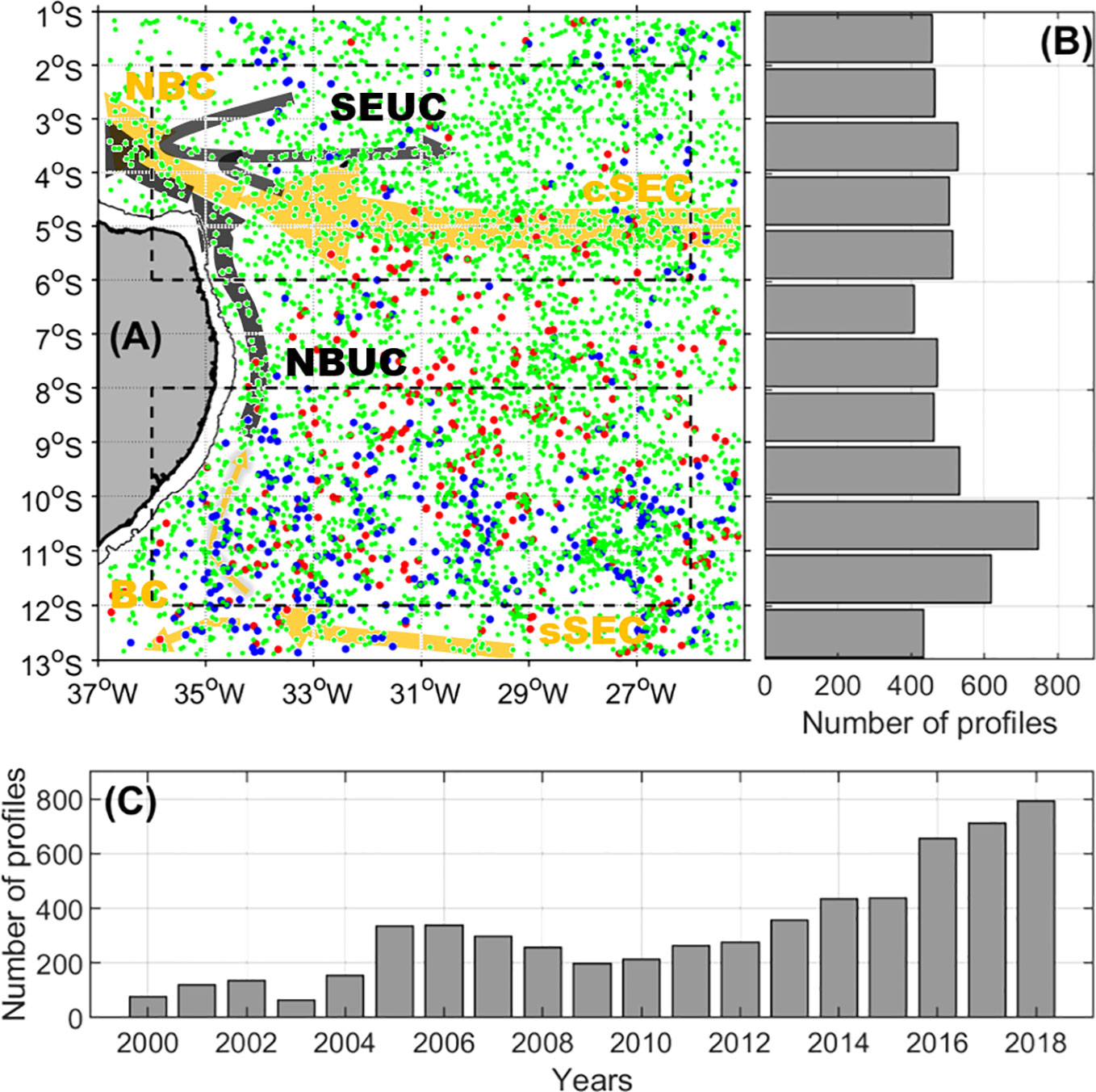
Figure 1 Spatio-temporal distribution of the 6134 Argo valid profiles used in this study. (A) Position of Argo profiles and schematic representation of mean currents off northeast Brazil. Blue (red) dots indicates Argo profiles inside CE (AE). Green dots indicate Argo profile outside eddies (AE & CE). Solid orange (black, respectively) lines indicate surface (subsurface) currents. sSEC, southern branch of South Equatorial Current; cSEC, central branch of South Equatorial Current; BC, Brazil Current; NBC, North Brazil Current; NBUC, North Brazil Undercurrent; SEUC, South Equatorial Undercurrent. (B) Meridional variation of the number of valid Argo profiles in one-degree latitudinal bands. (C) Yearly variation (2000-2018) of the number of valid Argo profiles.

In the western STAO, very few studies emphasized the mesoscale activity. Using a series of XBT data Bruce (1984), observed mesoscale eddy occurrence off North Brazilian coast. These eddies mostly occur in boreal summer and fall between 3°-10°N and can extend up to 300 – 400 m depth vertically. In the Northeast region, Silveira et al. (1994) was the first to observe a clockwise recirculation of the cSEC at the surface, when it approaches the northeast Brazil coast at ~33°W. However, the authors suggested that it might be occasional and seasonal. Then, based on numerical simulations, Silva et al. (2009) pointed out the high surface mesoscale activity along the cSEC patches close to the northeast Brazil region. More recently, mesoscale activity was studied in the region based on altimetry data at specific periods (Dossa et al., 2021; Silva et al., 2021). However, to the best of our knowledge, no study provided a general vision of the characteristics of mesoscale activity and its seasonal variation in northeast Brazil (NEB). Here, we took advantage of 26 years of altimetry data to determine the origin, occurrence and characteristics of mesoscale eddies within the NEB. We depicted the presence of two regions with different characteristics. The region of the Fernando de Noronha ridge was characterized by the dominance of cyclonic eddies while in the region where the sSEC bifurcates both cyclonic and anticyclonic eddies occurred comparably. Moreover, we reveal that there is no any connection between the eastern tropical Atlantic and the NEB.

Data and methods

Altimetry data and eddy tracking

To investigate mesoscale activity off northeast Brazil, we used altimetry observations including absolute dynamic topography (ADT) and derived surface geostrophic velocities data available from January 1993 to December 2018. These data were produced by Ssalto/DUACS multi-mission products with support from CNES (http://www.AVISO.altimetry.fr/duacs/). Multi-mission products refer to the combination of all satellites data available at one time: Jason-3, Sentinel-3A, HY-2A, Saral/AltiKa, Cryosat-2, Jason-2, Jason-1, T/P, ENVISAT, GFO, and ERS1/2. This dataset is mapped daily onto a 0.25° × 0.25° latitude/longitude grid (Ablain et al., 2015; Dupuy et al., 2016) and distributed by the Copernicus Marine Environment Monitoring Service (CMEMS: http://marine.copernicus.eu).

Mesoscale eddy identification is based on ADT daily maps, using the eddy detection algorithm from Chaigneau et al. (2008; Chaigneau et al., 2009). This algorithm finds the possible eddy centres corresponding to local extrema of ADT (maxima for AE, minima for CE), and defines the outermost closed contour around these extrema as eddy edges. Most previous studies on mesoscale eddies, have based eddy detection on sea level anomaly (SLA) fields because of inaccuracies in the geoid definition. However, recent improvements in estimation of the Mean Dynamic Topography, depending on the geoid (Rio et al., 2011; 2014) allowed to provide more accurate ADT fields. Thus, following Laxenaire et al. (2018) and Aguedjou et al. (2021), and the recommendations of Pegliasco et al. (2021), mesoscale eddies were detected on ADT fields instead of SLA. Eddy trajectories were then reconstructed using the tracking method developed by Pegliasco et al. (2015).

For each detected eddy, several properties were computed. The eddy amplitude corresponds to the absolute value of the difference between the ADT at the eddy centre and at the eddy edge. In our study, only eddies with amplitudes higher than 1 cm were retained. The eddy radius corresponds to the equivalent radius of a disk having the same area than the eddy. Only eddies with radii larger than 25 km were retained. The eddy kinetic energy (EKE) was computed as the average EKE inside the eddy, based on the geostrophic velocity components. Eddies with lifetime higher than 14 days were retained in the present study.

Relative vorticity (ζ ) of large-scale currents is determined from the zonal (U) and meridional (V) geostrophic velocity components as:

$\begin{array}{ll}\zeta = \frac{\partial V}{\partial x}- \frac{\partial U}{\partial y}& (1)\end{array}$

Barotropic instability, associated with the change of sign of the gradient of absolute vorticity (C), could drive eddy generation (Johns et al., 1990; Aguedjou et al., 2019). Indeed, it occurs in the region with weak value of C. As in Aguedjou et al. (2019), we computed the gradient of absolute vorticity as:

$\begin{array}{ll}C= \overrightarrow{\nabla } \left(f+\zeta \right).\overrightarrow{n}& (2)\end{array}$

where $\overrightarrow{n }= \frac{\overrightarrow{\nabla \left(\psi \right)}}{\left(\parallel \overrightarrow{\nabla \left(\psi \right)}\parallel \right)}$ is the unit vector perpendicular to geostrophic streamlines, $\psi = -\frac{g}{f}ADT$ is the stream function, f is the Coriolis parameter, g the gravitational acceleration.

To investigate eddy occurrence off Northeast Brazil (NEB) (37°-25°W;13°-1°S), we first build maps of spatial distribution of the number of detected eddies, eddy polarity, eddy properties (radius, amplitude), EKE, as well eddy speed of propagation and eddy life time. Eddy mean properties are accessed after gridding the region onto on 1° × 1° cells. The mean eddy properties correspond to the mean of all eddy-like features with lifetime > 14 days that occur in each cell. The analysis was performed over the study period (January 1993 - December 2018). Eddy number maps were built by considering the number of eddies with lifetime > 14 days within each cell. These maps show individual observations of eddies. For instance, if an eddy is stationary within a cell for 4 days, it will count as four observations within that cell. The eddy polarity is the probability for an eddy to be a cyclone (polarity < 0) or an anticyclone (polarity >0) and is defined as follow (Chaigneau et al., 2009):

$\begin{array}{ll}P = \frac{N_{AE}-N_{CE}}{N_{AE}+N_{CE}}& (3)\end{array}$

where N_AE is the number of AE while N_CE correspond to the number of CE.

Mean EKE maps correspond to the average mean EKE of eddy detected in each cell over the period of study.

Mean propagation maps of eddy were also built by considering the mean propagation speed of eddies with lifetime > 14 days within each cell. The eddy speed within each grid cell corresponds to the mean propagation speed of all eddy detected in each grid cell. Note that the eddy speed is the speed of a detected eddy from its location at time t to its next location at time t+1.

Argo dataset and classification of Argo profiles

To investigate the vertical structure of mesoscale eddies in the NEB region; we used the available Conductivity Temperature Depth (CTD) profiles acquired from autonomous floats of the Argo international program. These temperature and salinity vertical profiles are available at https://www.coriolis.eu.org/Observing-the-Ocean/ARGO. Vertical profiles from the Argo program in the Tropical Atlantic are available after 2000 (e.g., Aguedjou et al., 2021), reason why we limit our analysis to 2000-2018.

The mean thermohaline structure was first investigated by estimating the mixed layer depth (MLD), the isothermal layer depth (ILD) and the upper and lower limits of isothermal, halocline and pycnocline layers. The MLD was estimated using the criterion recently applied in the region (e.g., Araujo et al., 2011; Assunção et al., 2020). The MLD corresponds to the depth where the density is equal to the density at the reference depth (10 m), plus an increment corresponding to temperature change of 0.5 °C. The ILD was estimated using the same temperature criterion, assuming that it correspond to the depth where the temperature was 0.5°C below the temperature at the reference depth. The upper limit of the thermocline and the halocline/pycnocline corresponds to ILD and MLD respectively while the lower limit of both corresponds to the depth where the buoyancy frequency (N²) ≥ 10^-4 (Assunção et al., 2020).

Then, a composite analysis of the eddy vertical structures were performed following Aguedjou et al. (2021). First, we retained only vertical profiles with at least 30 data between 15 m and 950 m depth, and with no significant vertical gap between each data (see Aguedjou et al. (2021) for more details). In the study region, 6134 profiles were retained (Figure 1). Second, these profiles were classified into three categories, whether they surfaced inside AE, CE or outside eddies. In average, between 400 and 500 profiles are available in each band of one degree of latitude (Figure 1B), and a maximum of 730 profiles were acquired between 11°S and 12°S (Figure 1B). The temporal distribution shows that the number of profiles was less than 200 between 2000 and 2004 (Figure 1C). The number of profile decreased from 334 in 2005 to 198 in 2005, from where it linearly increased to 800 in 2018.

Wind data

Wind data were used to investigate the contribution of wind stress and wind stress curl in the formation of mesoscale eddies in the study region. The wind dataset used in the present study is the quality-assured monthly update of the ECMWF Reanalysis v5 (ERA5) available from 1979 to 2019 on the grid 0.25° x 0.25°. The dataset includes zonal and meridional wind component estimated at 10 m above sea level. The data is produced by Copernicus Climate Change Service (C3S) and is available at https://www.ecmwf.int/en/forecasts/datasets/reanalysis-datasets/era5. We used zonal and meridional component of the wind to estimate the wind stress and the wind stress curl within the northeast Brazil. The wind stress and its curl were estimated based on Gill and Adrian (1982) and considering a non-linear drag coefficient from Large and Pond (1981) modified for low wind speed (Trenberth et al., 1990).

Surface current data

To provide a more comprehensive picture of upper layer’s dynamic, we used the near-surface velocities climatological data derived from Global Drifter Program (GDP). Velocities are obtained from satellite-tracked drifting buoys drogued at 15 m depth. The climatology was built from dataset spanning from 1979 to 2015. The data were low-pass filtered to remove high-frequency currents and oscillations associated with local inertial periods. The data is monthly available on the grid 0.25° x 0.25°. This climatology is an update version of the older version described in Laurindo et al. (2017) (https://www.aoml.noaa.gov/phod/gdp/mean_velocity.php).

Results

Eddy density and mean properties off northeast Brazil

In the NEB, about 1500 eddies with radius larger than 25 km, amplitude larger than 1 cm and lifespan longer than 14 days were identified including 40% (60%) of AE (CE). The spatial distribution of mean annual number (1993 - 2018) of detected eddies (Figure 2A) revealed that eddies are much more numerous south of 8°S where up to 50 eddies per square degree per year were identified than north of 6°S (≤11 eddies per square degree). Considering this main feature, we defined two regions, the northern region A (36-26°W; 6°S-2°S) and the southern region B (36°-26°W; 8°-12°S).

FIGURE 2

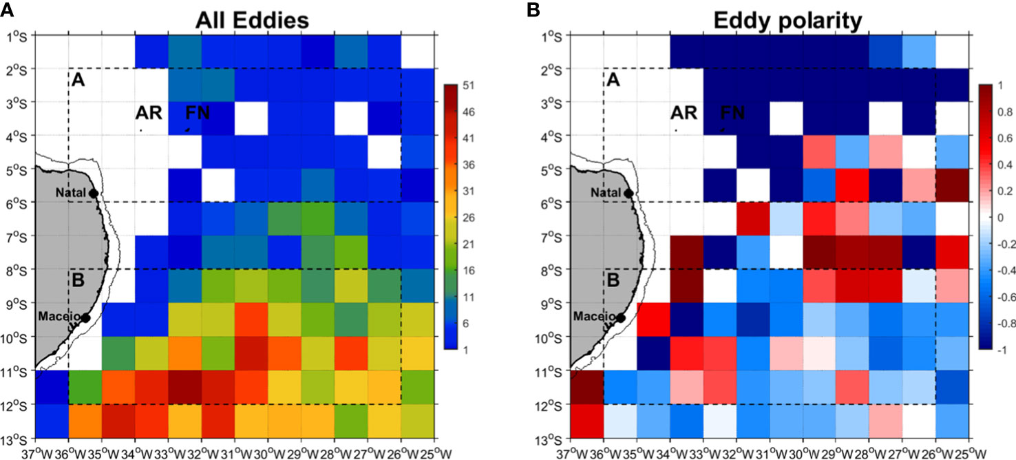
Figure 2 Spatial distribution of mean annual number of detected eddies per degree square over 1993-2018 period: (A) all eddies, (B) eddy polarity. The dashed rectangles delimit the northern (region A) and southern (region B) part of the NEB. The northern region A includes the Atoll das Rocas (AR) and Fernando de Noronha (FN) archipelago. The black solid line indicates the bathymetric contour at 70 m.

In region A, CE eddies were strongly dominant (85% CE and 15% AE) with a mean polarity that can reach -1 in some cells (Figure 2B). In region B, the proportion of AE and CE was alike (58% CE and 42% AE) with the polarity that can locally reach 1 or -1.

Eddy amplitude ranged between 1 and 2 cm with no clear spatial pattern (Figure 3A). Eddy radii ranged between 25 and 205 km with radii decreasing from North (> 110 km) to South (Figure 3B) in agreement with the decrease of the Rossby radius of deformation. EKE was much stronger in the equatorial region, North of 5°S, where it reached 210 cm² s^-2 than in region B where it was < 70 cm² s^-2 (Figure 3C). The mean meridional variation of eddy characteristics shown that eddies formed north of 3°S have higher mean characteristics (Figure 3D).

FIGURE 3

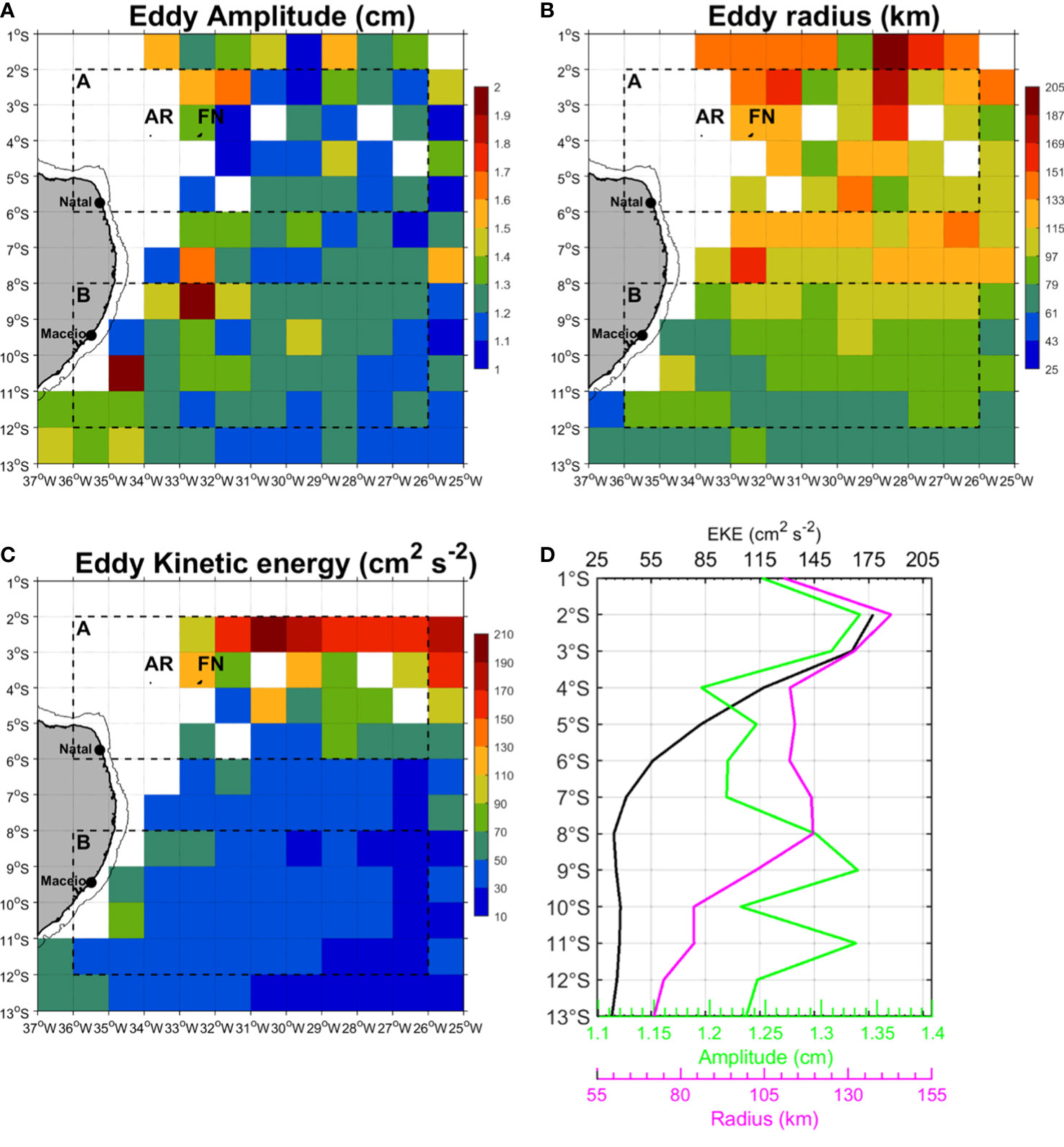
Figure 3 Spatial distribution of mean eddy characteristics per degree square over 1993 -2018 period: (A) eddy amplitude (cm), (B) eddy radius (km), (C) eddy kinetic energy (cm² s^-2) and (D) mean meridional variation of eddy characteristics.

Eddy genesis and propagation off northeast of Brazil

We detected and analysed 1950 eddy trajectories crossing the NEB (60% of CE and 40% of AE). About 25% of these eddies were formed outside the NEB mainly to the east from where they propagated westward into the study region, due to the beta effect (Figure 4). In region A, very few eddy trajectories were detected and they were mostly CE (85%). No AE propagated along the Fernando de Noronha Ridge. In contrast, most of eddy trajectories were concentrated in region B. In the near-coastal zone of region B, from the shelf-break to about 30 km offshore, only AE trajectories were observed.

FIGURE 4

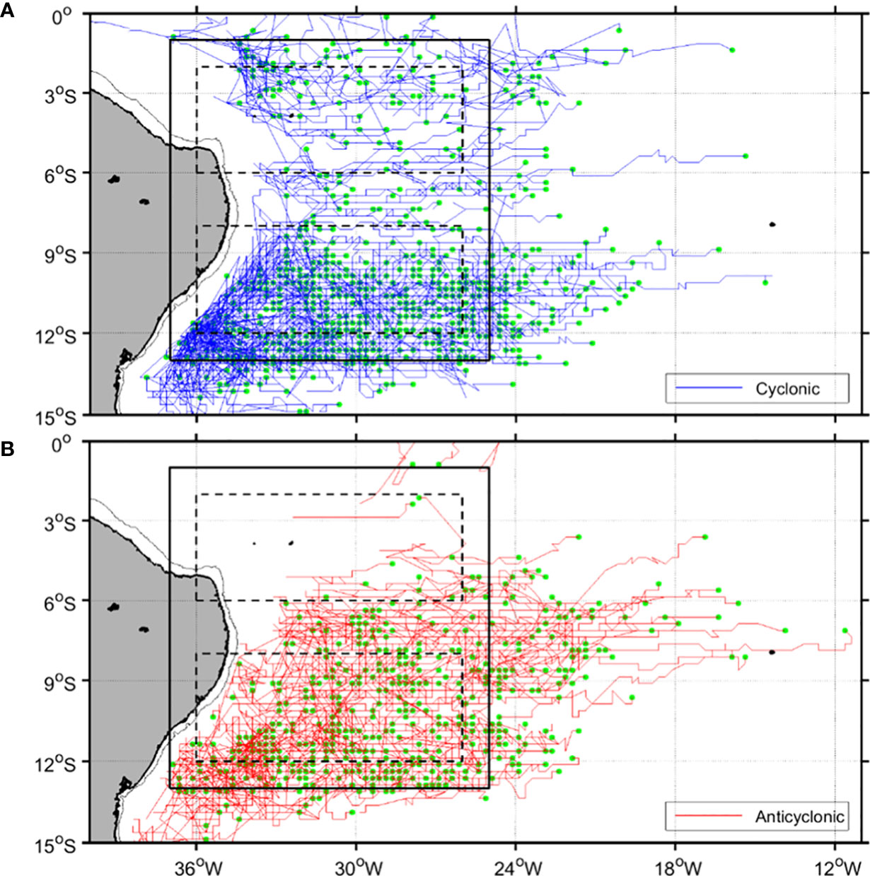
Figure 4 Trajectories of (A) cyclonic and (B) anticyclonic eddies which crossed the Northeast Brazil (NEB) region between January 1993 and December 2018. Green dots indicate the positions where these eddies were first identified. Black boxes indicate the NEB region while dashed boxes show regions (A, B) as in Figure 3.

Over the NEB region, eddies mostly propagate westward (Figure 5A). They were faster (> 10 cm s^-1) and less persistent (< 30 days) in region A than region B (< 10 cm s^-1; > 30 days). Eddies formed near the shelf-break west of 33°W had relatively low velocities and short lifetimes likely due to the interaction with the coast. Eddies within NEB lasted more when they have weak speed of propagation (Figure 5B).

FIGURE 5

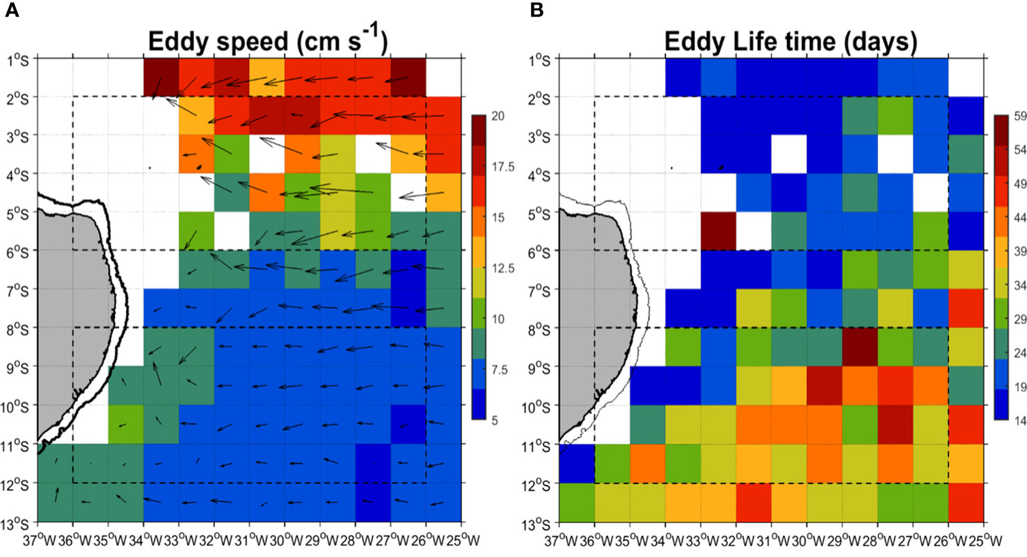
Figure 5 Spatial distribution per degree square over 1993-2018 period of (A) mean eddy propagation speed (colors) and direction (arrows) and (B) mean eddy life time off northeast Brazil.

Eddy properties within the NEB and regions A and B are summarized in Table 1. On average, 1950 eddies trajectories crossed the NEB between 1993 and 2018. They are subdivided into 775 AE and 1173 CE. Among, these eddies, 1470 (583 AE, 887 CE) were generated within the NEB. The average amplitude of both type of eddies are alike (~ 1.3 cm). However, CE exhibited greater average EKE (51 cm s^-2) than AE (35 cm s^-2). In region A, only 175 eddy trajectories (41 AE, 134 CE) passed within the region over the period of study while only 94 eddies were formed in the region over the same period. Both types of eddy formed in region A have alike average amplitudes. However, CE have greater average radius, EKE, speed than AE. On other side, 1114 eddy trajectories crossed the region B including 448 AE and 666 CE. Among these eddies, 768 (326 AE, 442 CE) were formed within the region before propagating out of the region or decaying within it. Both type of eddies have alike amplitude (1.2 ± 0.3 cm for AE; 1.3 ± 0.5 for CE). Average radius for AE was greater (91.4 ± 29 km). However, CE exhibited greatest lifetime (41 ± 29 days).

TABLE 1

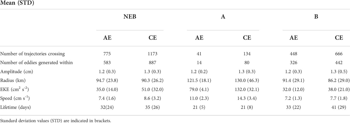
Table 1 Mean properties and characteristics of AE and CE within NEB and northern part of NEB (A) and southern part of NEB (B).

Eddy seasonal variability and mechanisms behind its formation off northeast Brazil

In the NEB region, CE dominated over AE throughout the year except in June when the proportion of both types were alike (Figure 6) This seasonal variation is similar with the observation of Bruce, 1984 in the northern latitude (3- 10°N). However, the seasonal variation was alike for both types of eddies with a maximum in August-September and minimum in February-March (but a local minimum in June for CE).

FIGURE 6

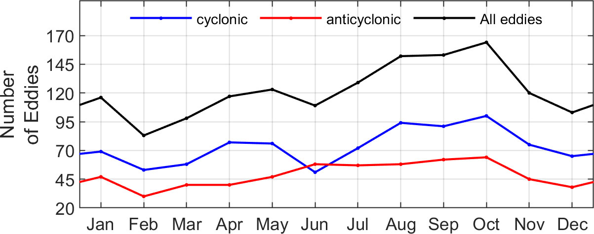
Figure 6 Seasonal cycle of the number of eddies generated off Northeast Brazil.

We further estimated the seasonal variation of the number of AE and CE as well as the wind stress curl and wind stress magnitude by region. In region A, CE dominated AE from April to November with a peak in October while between December and March the proportion of both eddies was alike (Figure 7A). The seasonal variation of CE in this region seems related to the seasonal variation of wind stress curl (Figure 7A). The wind stress curl was negative throughout the year within region A. Between June and October; it shows similar variations as the number of CE, increasing from -1.6×10^-8 N m^-3 in June to 0.8×10^-8 in October. On other side, the magnitude of the wind stress exhibited a clear seasonal cycle (Figure 7C) within region A from less than 0.03 N m^-2 in March-April to 0.06 N m^-2 in August-September.

FIGURE 7

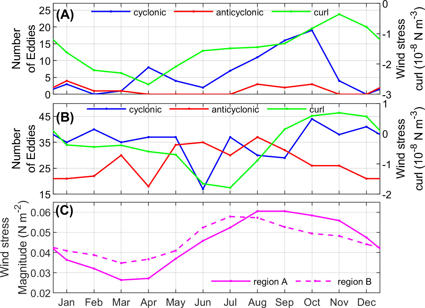
Figure 7 Seasonal cycle of (A) number of AE and CE (red and blue lines respectively) and wind stress curl (green line) within northern part of NEB (region A), (B) number of AE and CE (red and blue lines respectively) and wind stress curl (green line) within southern part of NEB (region B), and (C) wind stress magnitude in regions A (magenta solid line) and B (dashed magenta line).

In region B, less seasonal variation was observed for the number of both eddy types (Figure 7B). However, AE and CE were respectively minimum in April and June and maximum in August and October. The wind stress curl within the region showed a clear seasonal variation. Two distinct periods of variability were observed: a negative wind stress curl between January and August and a positive wind stress curl between September and December. The maximum wind stress curl (0.7×10^-8 N m^-3) occurred in November while the minimum wind stress curl (- 1.7×10^-8 N m^-3) occurred in July. On other side, wind stress magnitude depicted a clear seasonal variation (Figure 7C), increasing from ~0.035 N m^-2 in March to ~0.06 N m^-2 in July. In both regions, the wind stress curl and the wind stress seem to contribute to the generation of eddies. However, other mechanisms could induce eddy formation in the region.

Indeed, several other mechanisms such as the topographic effect, barotropic and baroclinic instabilities are susceptible to promote the formation of eddies in the world ocean. According to the Rayleigh (1880) criterion extended to nonparallel steady currents and applied in the geostrophic context, barotropic instabilities increase in regions where the gradient of the absolute vorticity (C) of large-scale currents almost vanished. This criterion was recently applied in the region of the NECC retroflection in the tropical Atlantic (Aguedjou et al., 2019) where more than 55% of eddies are formed in areas of weak vorticity gradient. In the same way, we first estimated the seasonal cycle (1993 – 2018 monthly mean maps) of the gradient of absolute vorticity gradient superimposed with the formation position of each eddy detected in regions A and B (Figure 8). In a second step, we assessed the variation of the number of eddies formed in each region as a function of the absolute vorticity gradient (Figure 9).

FIGURE 8

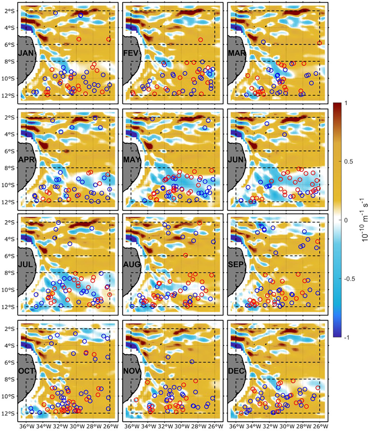
Figure 8 1993 – 2018 monthly mean maps of gradient of absolute vorticity of large-scale currents (color shading) superimposed with eddy location of long-lived eddies generated off northeast Brazil between 1993 and 2018 (blue and red circles for cyclonic and anticyclonic eddies respectively).

FIGURE 9

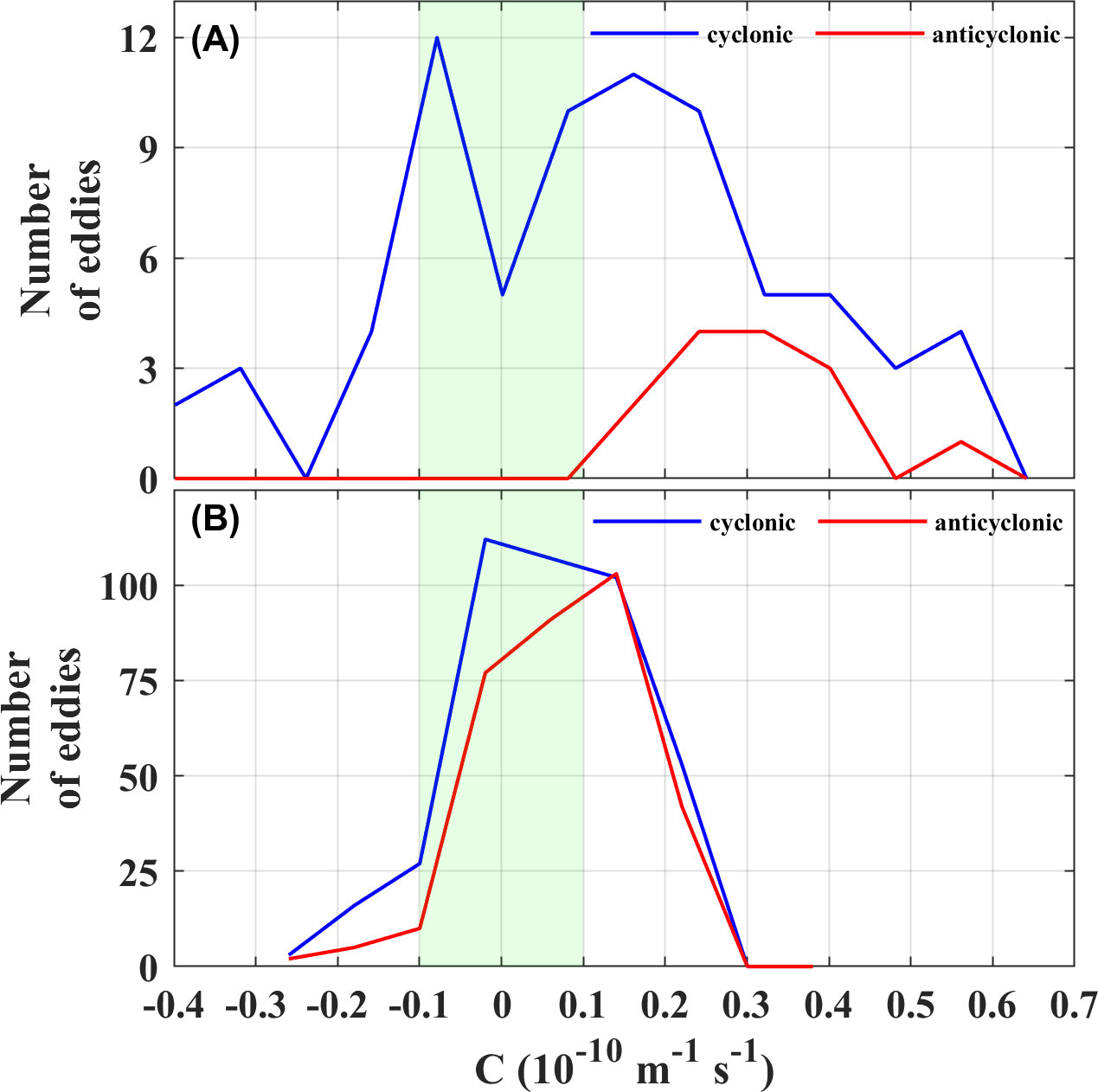
Figure 9 Distribution of the number of detected cyclonic and anticyclonic eddies as function of the gradient of large-scale absolute vorticity C at eddy generation sites for all eddies generated between 1993 and 2018 within: (A) northern part of NEB (region A) and (B) southern part of NEB (region B). Green vertical in (A, B) indicate interval values C within ± 0.1×10^-10 m^-1 s^-1.

The NEB region was dominated by large positive vorticity values throughout the year. Nevertheless, negative gradient values can be observed in some areas (Figure 8). In region A, the distribution did not show a well pronounced seasonal cycle. The region was dominated by positive gradients. However, intense positive values can be observed in some areas. For example, at the northern limit of the region along 2°S, at ~30-25°W, a positive intensification of gradient was observed from January to August, but disappeared in September-October before reappearing in November. At the western limit of the region (36-35°W) at ~ 4 - 3°S, a negative intensification superimposed by a positive intensification was observed all year long. Still, in some places, we can observe some strong positive values of vorticity gradient.

During the first trimester (January-March), very few eddies were formed in the area. Among these, we observed just two CE in January that were formed in areas of gradient close to zero. Between April and October, most of eddies (AE, CE) were formed in low gradient areas.

In the southern part of NEB, in region B, the spatial distribution of the gradient of absolute vorticity showed a strong seasonal cycle. Between April and August, the region was dominated with negative gradient of absolute vorticity, which was much extended during June – July. Between September and March, when the gradient within the region was dominantly positive, very few eddies were generated in the area of weak gradient. Therefore, a better estimation of number of eddies generated within region of weak gradient is necessary. For this purpose, we provided the mean number of eddies generated within regions A and B in function of gradient of vorticity at position of each detected eddy (Figure 9).

In region A, 34% of CE were formed within areas where the gradient of absolute vorticity (C) was close to zero (± 0.1×10^-10 m^-1 s^-1) (Figure 9A) while only one AE was formed in regions of weak C. Therefore, others mechanisms may be involved into the formation of both types of eddies within this region. In the southern part of NEB, in region B, most eddies were generated within areas of weak gradient of vorticity (Figure 9B). Among CE formed in the region, ~57% were formed in region of weak C (± 0.1×10^-10 m^-1 s^-1) against 54% for AE. Hence, barotropic instabilities mostly control eddy formation in region B. Due to the complex dynamics of the region, the horizontal shear of the surface currents could also contribute to the formation of eddies off NEB.

Surface current analysis from near-surface drifter data provides information on upper layer dynamics. It revealed a dominant zonal current north of 5°S (Figure 10). Along the coast, current velocities exhibited a seasonal variability. They intensified progressively from January to July with the occurrence of strong values in May-June when the speed can reach 1 m s^-1 north of 5°S and 0.8 m s^-1 south of 8°S. These velocities along the coast weakened from July to December.

FIGURE 10

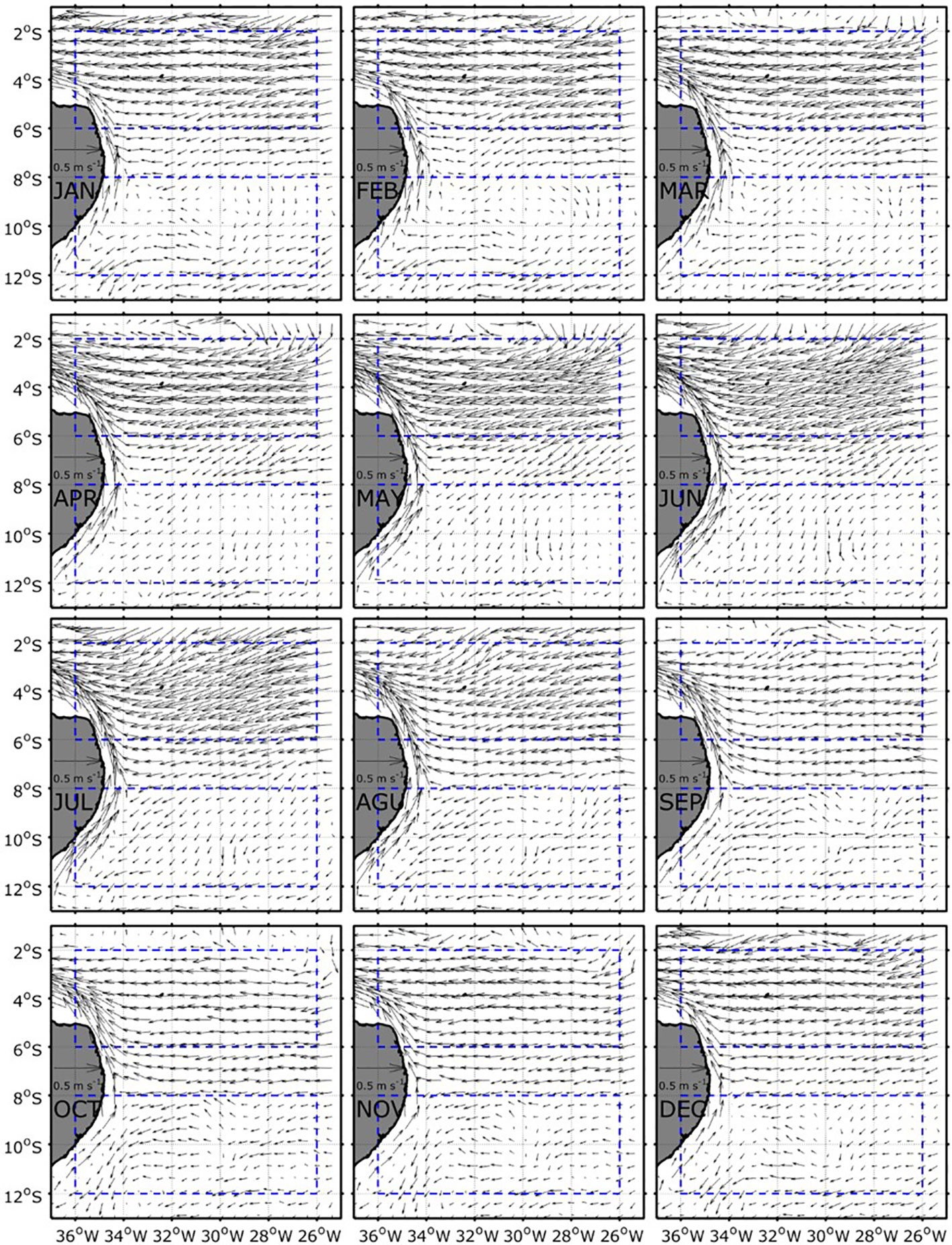
Figure 10 Mean monthly (1979 - 2015) map of surface currents from drifter off NEB.

In region A, the circulation was mainly westward (characteristic of the cSEC) at the beginning of the year (January-February-March). In April, the current velocities strengthened (>0.8 m s^-1). During this month, a cyclonic recirculation around 2°S between 26°-30°W was noted at the northern limit of the region, and remained permanent until May, when it gradually disappeared. From May onward, the circulation slightly changed of direction and progressively shifted to the southwest around 3°S, East of 28°W. This orientation became noticeable in most of the region until August. However, from this month, the strength of the current weakened in the region and became westward until the end of the year.

On the other hand, the current velocities in region B were weaker than those in region A throughout the year. Moreover, the circulation was not as organized as in region A. Early in the year, cyclonic structures were observed around 28°W between 10°-8°S. In addition, around 10°S to about 34°W, there was a retroflection of a zonal flow from the east, remarkable from February. During the retroflection, the zonal flow split in two, one was directed to the north and the other to the south. This southward flow recirculates further south and enter into the northward coastal flow. In April, we noticed that the retroflection occurred a little further north around 8°S, while the recirculation of the southward flow occurred around 10°S. This retroflection remains permanent around 8°S throughout the year. On the other hand, the cyclonic recirculation of the southward flow occurred progressively further south. In July-August, it was quite remarkable around 12°S to ~36°S. Between September and December, it occurs much more to the south. In addition, east of the region at 10°-8°S; 30-28°W, a meander of the surface current was present between August and September.

Eddies connecting eastern and western tropical Atlantic

To investigate possible connection between the northeast Brazil and the eastern tropical Atlantic we used the trajectories crossing three key distinctive regions along the western tropical Atlantic (Figure 11). Few eddy trajectories formed in the tropical Atlantic (40° S- 40°N; 60° W- 30°E) crossed the Amazon River plume (AMZ) (Figure 11A). Most trajectories observed in the region were originated within the region. Very few AE trajectories originated from the eastern Atlantic crossed the AMZ while no CE trajectories originated from the eastern coast crossed it (Figure 11A). South of the AMZ, off the NEB, most trajectories were originated within the region. No eddy trajectories (AE, CE) originated from the eastern tropical Atlantic were observed. The region thus does not have any connection with the eastern tropical Atlantic through mesoscale eddies. Finally, a clear connection between the southeastern Atlantic and the southwestern tropical was revealed (Figure 11C), in agreement with Laxenaire et al. (2018). The connection was mostly made through AE, with up to 8 trajectories originating from the southeastern tropical Atlantic (east of 7°E). On other side, only one CE originated from the southeastern Tropical Atlantic crossed the basin.

FIGURE 11

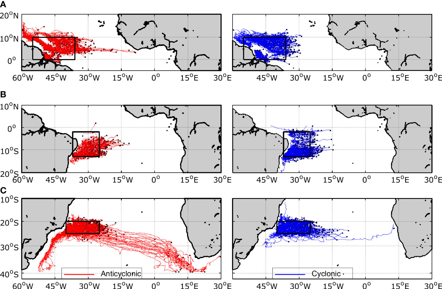
Figure 11 Mesoscale eddy trajectories detected in the tropical Atlantic crossing the: (A) Amazon river plume region (55°– 36°W; 0° – 10°N), (B) northeast Brazil region (37° – 25°W; 13° - 2°S) and (C) southwestern tropical Atlantic (40° – 25°W; 25° - 20°S). Red (blue) lines indicate AE (CE) trajectories. Black dots indicate eddy generation position.

Eddy vertical extent

In order to study eddy vertical extent in the NEB, we first provide the mean temperature, salinity and density profiles from Argo floats in regions A and B (Figure 12). In region A, The MLD and the ILD were respectively 51 m and 56 m. The temperature profile was characterized by relatively weak stratification above 200 m with thermocline extending from 56 to 146 m depth while halocline and pycnocline extending between 51 and 146 m depth (Figure 12A). In region B, the MLD and the ILD were 55 m and 63 m, respectively (Figure 12B). The mean temperature, salinity and density profiles exhibited low stratification, characterized by thermocline extending from 63 m to 185 m depth. The halocline/pycnocline ranged at 55 – 185 m depth.

FIGURE 12

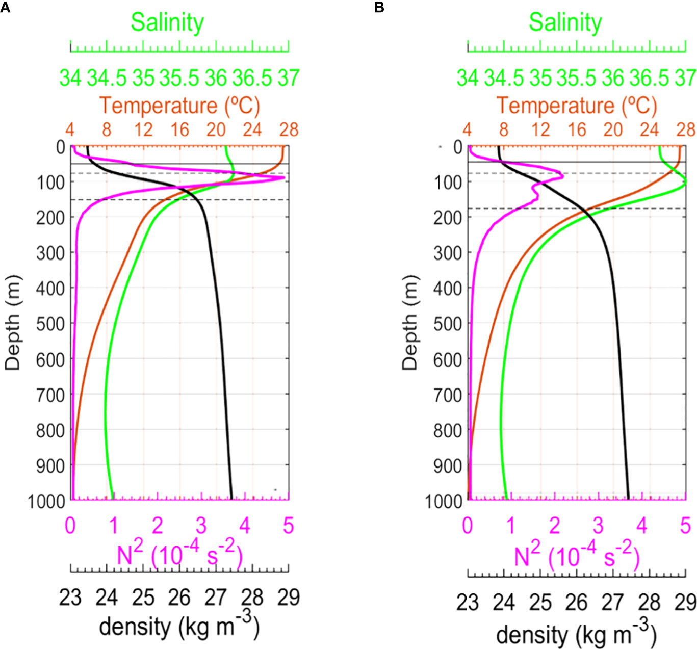
Figure 12 Mean Temperature, salinity, density, and squared buoyancy frequency (N²) inside eddies in the regions (A, B) Solid horizontal line indicates the base of the mixed layer depth while the dashed horizontals lines indicate the upper and lower thermocline depth. The lower thermocline depth also corresponds to the pycnocline depth.

In region A and B, vertical profiles of the mean temperature, salinity and density anomalies were largest within eddies than outside eddies (Figure 13). In region A, the largest mean temperature anomalies (> 0.2°C) in AE were located at ~ 60 – 180 m depth, with a maximum anomaly of 1.4°C at 105 m depth (Figure 13A). The corresponding salinity anomalies were weaker in AE (< 0.1). Salinity anomalies inside AE were negative above 85 m depth. Below this depth, at ~ 85 – 220 m, the anomalies were positive, with largest values (> 0.01) observed between 90 m and 190 m depth. The maximum anomaly (0.09) was reached at ~135 m depth. Below 220 m depth, the anomaly changed sign and became slightly negative. Inside CE, temperature anomalies were mostly positive (Figure 13A) and largest temperature anomalies (< -0.1°C) were observed between ~ 40 and 230 m depth, with an extremum (-1.25°C) at 90 m depth. The corresponding salinity anomalies were positive above 65 m depth, but the highest anomalies in absolute value located practically at the same depth. The extremum in salinity anomaly was reached at 115 m depth. Profile of mean density anomalies were mostly consistent with the temperature anomaly profiles (except in the upper surface layer), demonstrating that in region A, the density distribution is mostly driven by temperature changes. As expected outside eddies, the mean temperature, salinity, and density anomalies were almost null.

FIGURE 13

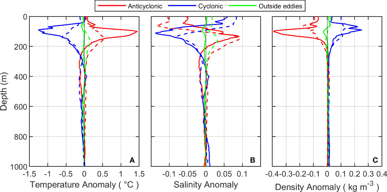
Figure 13 Mean vertical profiles of (A) temperature anomaly, (B) salinity anomaly, and (C) density anomaly in regions A and (B) Solid lines (dashed lines) correspond to the mean profiles obtained in region A (B) for the composite CE (blue lines), AE (red lines) and outside eddies (green lines).

In region B, above 200 m depth, the mean temperature, salinity, and density anomalies within (outside) both types of eddy were weaker (higher) than in region A. Inside AE of region B, the highest temperature anomalies (> 0.2°C) were located at ~60- 230 m depth, with an extremum (0.5°C) at 155 m depth. The corresponding salinity anomalies were negative above 105 m. Below this depth, these anomalies become positive along with the depth until ~800 m depth where they almost vanished. The largest positive anomalies (0.01) ranged at ~100 – 270 m depth, with an extremum (0.09) at 150 m depth. In the CE of the region, the highest temperature anomalies in absolute value (> 0.2 °C) were observed at ~ 60 – 230 m depth with an extremum (-0.6) at 140 m. Salinity anomalies were also positive in the near-surface layer (above 90 m) and below 890 m depth (Figure 13B) and were maximum (> 0.01) at ~110 – 270 m depth. On other side, the profile of mean density anomalies was similar with the profile of mean temperature anomalies (Figures 13A, C), demonstrating that change in temperature also controlled most of the density distribution in region B. Mean sea water properties and associated anomalies at depth where the density is maximum are summarized in Table 2.

TABLE 2

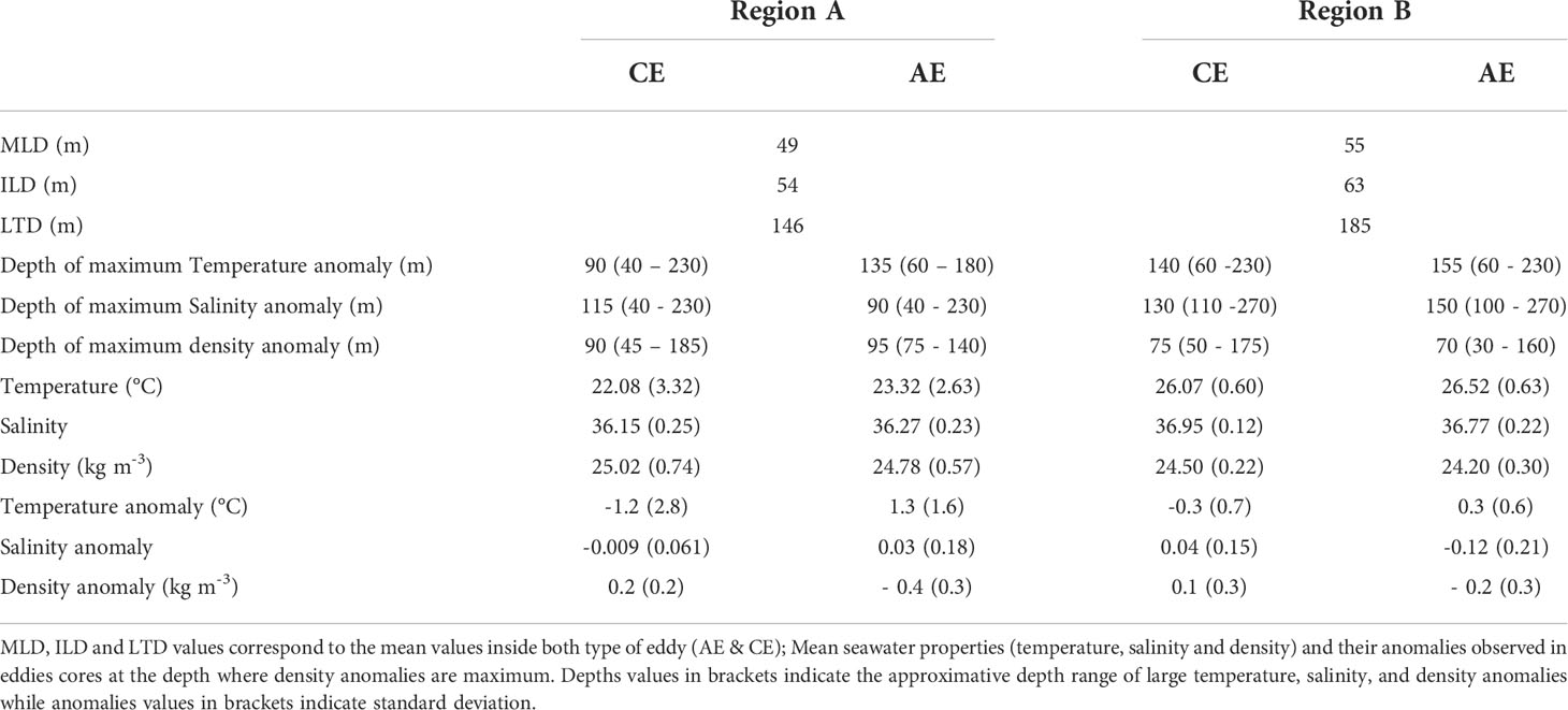
Table 2 Depths of mixed layer, isothermal layer, lower thermocline limit, maximum temperature anomaly and maximum salinity anomaly inside eddies in region A and B.

The definition of the lower limit of the eddy extent in the water column is a challenging task. In the present study, we based our definition on the isotherm and isohaline threshold. Following Sandalyuk and Belonenko (2021), we defined the lower limit of eddy extent as the depth where both temperature and salinity anomalies within eddies correspond to about 10% of the maximum anomalies. Using this criterion, we observed that in region A, AE (CE) lower limit is located at ~ 180 m (250 m) while in region B, AE (CE) extended up to ~ 250 m (270 m).

Discussion and conclusion

Based on altimetry data and Argo data, this study characterized the mesoscale eddies and the possible mechanisms involved in their generation off Northeast Brazil. Gradients of absolute vorticity from AVISO geostrophic velocity fields allowed us to observe the contribution of barotropic instabilities in the eddy generation within the region of interest. Then, wind data from ERA5 and surface velocities data from near-surface drifters enabled us to emphasize the contribution of wind stress curl and dynamics of surface currents, respectively. In addition, an important finding is that mesoscale eddies do no directly connect the eastern tropical Atlantic to the NEB region.

Automatic eddy detection and tracking algorithms applied to daily ADT maps from January 1993 to December 2018 allowed us to reveal 1950 eddies trajectories crossing the NEB. Among these eddies, 1470 eddies (40% AE and 60% CE) were formed within the region of interest. There was no clear geophysical preference for both types of eddy in NEB as observed in the Global ocean (Chelton et al., 2011) and specifically in the tropical Atlantic (Aguedjou et al., 2019).

Our results reveal that in the northern part (region A), eddies are rather rare. They tend to have a large radius, a large EKE, low amplitudes and do not live too long. This is due to the baroclinic Rossby radius deformation (e.g., Chaigneau et al., 2009). CE dominate region A. Although barotropic instabilities can contribute to the formation of the CE in the region, negative wind stress curl associated with an increase intensity of wind stress seems to also favour their formation (Figures 7A, C, 8, 9) in accordance with Rodrigues et al. (2007) for the region.

More eddies were formed in the south (region B) than in the northern part of the NEB indicating that different physical processes control the eddy dynamics in each region. Indeed, in region A lies the Fernando de Noronha ridge, which encompasses seamounts, the Fernando de Noronha archipelago and Atoll das Rocas (Figure 2). It is also a region where the intense surface current NBC is formed when the cSEC crossing the region enters the western boundary system (e.g., Dossa et al., 2021). Most of eddies observed in this region were formed in the eastern part of the FN archipelago from where the cSEC flows (Figure 4A). West of AR, few eddy trajectories were observed, but none of them was formed in this region. This is not consistent with the theory indicating that the disruption of the current flow by the islands can induce the generation of eddies in the wake of the obstacle (e.g., Arístegui et al., 1997). This inconsistency may be because the altimeter resolution near the equator is too large and did not allow to capture eddies with lower amplitude. This suggests the need of Surface water and ocean Topography (SWOT) to access fine mesoscale geostrophic currents in near equatorial region, to better capture eddies in the region. Moreover, Silva et al. (2021) showed that the presence of the FN Archipelago induces strong disturbances of the cSEC with a splitting of its core upstream of the archipelago. They also highlighted the effect of the topography around islands on the intensity and direction of the currents, which can favour eddy generation at the wake of the FN archipelago. At the western extremity of region A, where one would expect eddy formation due to the interaction of the cSEC with the western boundary system, no eddies were observed because, eddies in this region have small life and propagate very fast.

More eddies (AE, CE) were observed in region B (Table 1). Several processes are likely to promote their formation. First, it is a region where lies the Pernambuco Plateau at ~8°S (Silva et al., 2022). The interaction of the large-scale currents with this plateau could generate eddies (e.g., Herbette et al., 2003). Dossa et al. (2021) showed that the northward meridional flow originating from the south of the region is slightly shifted eastward until ~7.5°S (northern extremity of the region) where it changes direction to the west as the coast orientation changes. This suggests that the formation of about five AE eddies observed in region B over the continental slope (Figure 4A) may be favoured by the interaction of near-coastal circulation with the topography.

Second, region B constitutes part of the sSEC retroflection zone (10°-14°S, Rodrigues et al., 2007) where the NBUC (BC) is formed and flows northward (southward). The latitude of the retroflection is subjected to south-north migration due to the change in wind stress curl (wind stress curl < 0 or > 0) near the coast (Rodrigues et al., 2007) which is favourable for the generation of eddies. Similarly, we observed that the negative wind stress curl between January and September observed within region B is correlated with the seasonal cycle of the number of CE (Figure 7B). Therefore, the negative wind stress curl likely contributes to the generation of CE formed in region B.

Third, barotropic instabilities also contribute to the formation of both types of eddies in region B. Almost 57% (54%) of the CEs (AEs) formed in this region, are generated in regions where the gradient of absolute vorticity is close to 0, justifying the strong contribution of barotropic instabilities associated with horizontal shear of surface currents in the region (Figure 10).

In both regions (A, B) of the NEB, the formation of both types of eddies seems to be driven not only by the mechanisms highlighted here (barotropic instabilities, wind stress curl, topographic effect), but other mechanisms such as baroclinic instabilities (e.g., von Schuckmann et al., 2008) could be involved in the eddy generation within NEB. The formation of eddies downstream of the islands and the topographic effect need to be investigated through a high-resolution numerical model to better understand their role in the formation of eddies.

Through eddy tracking algorithm in the tropical Atlantic, we did not observe any eddy connecting the eastern tropical Atlantic and the Northeast Brazil (Figure 11A). However, some mesoscale eddies originating from western Africa (southeastern boundary) can eventually propagate until the Amazon River plume (southwestern tropical Atlantic) (Figures 11B, C). The latter connection was also observed by Laxenaire et al. (2018). These authors have reported that anticyclonic eddies can travel from the Indian Ocean from where they carry salty and warm water to the southeastern Atlantic.

The composite analysis of Argo profile revealed that the occurrence of mesoscale eddies have an influence on thermohaline structure off northeast Brazil. In the northern region, CE tend to stretch the thermocline and the halocline vertically of 45 m in depth (Figures 12A, 13A, B and Table 2). AE only stretch the halocline and moved the thermocline 6 m in depth with a vertical extent of ~30 m (Figures 12A, 13A, B and Table 2). In the southern region, both type of eddy (AE & CE) have similar influence on the thermocline and the halocline. They tend to stretch to thermocline 45 m in depth and move the halocline 55 m in depth with an extent of ~50 m (Figures 12B, 13A, B and Table 2). Eddies plays same role on the thermohaline structure in the southern region, because, they have almost the same vertical extent (Table 2).

Data availability statement

All the data used in this study are publicly available. The altimetry datasets can be obtained from the Copernicus Marine Environment Monitoring service (CMEMS: http://marine.copernicus.eu). The sea surface velocities current from DRIFTER are available at https://www.aoml.noaa.gov/phod/gdp/mean_velocity.php. The wind datasets are publicly available at https://www.ecmwf.int/en/forecasts/datasets/reanalysis-datasets/era5. Argo profiles are available at https://www.coriolis.eu.org/Observing-the-Ocean/ARGO.

Author contributions

AND, AS and AB conceptualized the work. AND, HA and AC worked in data processing. AND provided the original draft. All authors contributed to the article and approved the submitted version.

Funding

This work was supported by the CAPES/PRINT (n° 88887.470036/2019-00) through a PhD internship scholarship grant for AND. This work was a contribution to the LMI TAPIOCA, the SMAC project (CAPES/COFECUB no. 88881.142689/2017–01), the PADDLE project (funding by the European Union’s Horizon 2020 Research and Innovation Programme—Grant Agreement 73427) and EU H2020 TRIATLAS project under Grant Agreement 817578.

Acknowledgments

This work was supported by the CAPES/PRINT (n° 88887.470036/2019-00) through a PhD internship scholarship grant for A.N.D. This work was supported by the CAPES (Coordenação de Aperfeiçoamento de Pessoal de Nível Superior) through a PhD scholarship grant for A.N.D. MA thanks the Brazilian Research Network on Global Climate Change—Rede CLIMA (FINEP-CNPq 437167/2016-0) and the Brazilian National Institute of Science and Technology for Tropical Marine Environments—INCT AmbTropic (CNPq/FAPESB 565054/2010-4 and 8936/2011) for their support. This work is a contribution to the In- ternational Joint Laboratory TAPIOCA (www.tapioca.ird.fr), to the SMAC project (CAPES/COFECUB n° 88881.142689/2017–01), the PADDLE project (funding by the European Union’s Horizon 2020 research and innovation programme - grant agreement No. 73427), and to the TRIATLAS project, which has also received funding from the European Union’s Horizon 2020 research and innovation program under grant agreement No 817578.

Conflict of interest

The authors declare that the research was conducted in the absence of any commercial or financial relationships that could be construed as a potential conflict of interest

Publisher’s note

All claims expressed in this article are solely those of the authors and do not necessarily represent those of their affiliated organizations, or those of the publisher, the editors and the reviewers. Any product that may be evaluated in this article, or claim that may be made by its manufacturer, is not guaranteed or endorsed by the publisher.

References

Ablain M., Cazenave A., Larnicol G., Balmaseda M., Cipollini P., Faugère Y., et al. (2015). Improved sea level record over the satellite altimetry era, (1993-2010) from the climate change initiative project. Ocean Sci. 11, 67–82. doi: 10.5194/os-11-67-2015

CrossRef Full Text | Google Scholar

Aguedjou H. M. A., Chaigneau A., Dadou I., Morel Y., Pegliasco C., Da-Allada C. Y., et al. (2021). What can we learn from observed temperature and salinity isopycnal anomalies at eddy generation sites? application in the tropical Atlantic ocean. J. Geophys. Res. Ocean 126, 1–27. doi: 10.1029/2021JC017630

CrossRef Full Text | Google Scholar

Aguedjou H. M. A., Dadou I., Chaigneau A., Morel Y., Alory G. (2019). Eddies in the tropical Atlantic ocean and their seasonal variability. Geophys. Res. Lett. 156–164. doi: 10.1029/2019GL083925

CrossRef Full Text | Google Scholar

Araujo M., Limongi C., Servain J., Silva M., Leite F. S., Veleda D., et al. (2011). Salinity-induced mixed and barrier layers in the southwestern tropical Atlantic ocean off the northeast of Brazil 63–73. doi: 10.5194/os-7-63-2011

CrossRef Full Text | Google Scholar

Arístegui J., Tett P., Hernández-Guerra A., Basterretxea G., Montero M. F., Wild K., et al. (1997). The influence of island-generated eddies on chlorophyll distribution: A study of mesoscale variation around gran canaria. Deep Res. Part I Oceanogr. Res. Pap. 44, 71–96. doi: 10.1016/S0967-0637(96)00093-3

CrossRef Full Text | Google Scholar

Arruda W. Z., Campos E. J. D., Zharkov V., Soutelino R. G., da Silveira I. C. A. (2013). Events of equatorward translation of the vitoria eddy. Cont. Shelf Res. 70, 61–73. doi: 10.1016/j.csr.2013.05.004

CrossRef Full Text | Google Scholar

Assunção R. V., Silva A. C., Roy A., Bourlès B., Silva C. H. S., Ternon J. F., et al. (2020). 3D characterisation of the thermohaline structure in the southwestern tropical Atlantic derived from functional data analysis of in situ profiles. Prog. Oceanogr. 187, 102399. doi: 10.1016/j.pocean.2020.102399

CrossRef Full Text | Google Scholar

Bruce J. G. (1984). Comparison of eddies off the north Brazilian and Somali coasts. J. Phys. Oceanogr. 14 (4), 825–832. doi: 10.1175/1520-0485(1984)014<0825:COEOTN>2.0.CO;2

CrossRef Full Text | Google Scholar

Campos E. J. D. (2006). Equatorward translation of the vitoria eddy in a numerical simulation. Geophys. Res. Lett. 33, 1–5. doi: 10.1029/2006GL026997

CrossRef Full Text | Google Scholar

Chaigneau A., Eldin G., Dewitte B. (2009). Eddy activity in the four major upwelling systems from satellite altimetry, (1992-2007). Prog. Oceanogr. 83, 117–123. doi: 10.1016/j.pocean.2009.07.012

CrossRef Full Text | Google Scholar

Chaigneau A., Gizolme A., Grados C. (2008). Mesoscale eddies off Peru in altimeter records: Identification algorithms and eddy spatio-temporal patterns. Prog. Oceanogr. 79, 106–119. doi: 10.1016/j.pocean.2008.10.013

CrossRef Full Text | Google Scholar

Chelton D. B., Schlax M. G., Samelson R. M. (2011). Global observations of nonlinear mesoscale eddies. Prog. Oceanogr. 91, 167–216. doi: 10.1016/j.pocean.2011.01.002

CrossRef Full Text | Google Scholar

Djakouré S., Penven P., Bourlès B., Veitch J., Koné V. (2014). Coastally trapped eddies in the north of the gulf of Guinea. J. Geophys. Res. Ocean 119, 6805–6819. doi: 10.1002/2014JC010243

CrossRef Full Text | Google Scholar

Dossa A. N., Silva A. C., Chaigneau A., Eldin G., Araujo M., Bertrand A. (2021). Near-surface western boundary circulation off northeast Brazil. Prog. Oceanogr. 190, 102475. doi: 10.1016/j.pocean.2020.102475

CrossRef Full Text | Google Scholar

Dufois F., Hardman-Mountford N. J., Greenwood J., Richardson A. J., Feng M., Matear R. J. (2016). Anticyclonic eddies are more productive than cyclonic eddies in subtropical gyres because of winter mixing. Sci. Adv. 2, 1–7. doi: 10.1126/sciadv.1600282

CrossRef Full Text | Google Scholar

Dupuy S., Pujol M.-I., Picot N., Ablain M., Faugère Y., Taburet G., et al. (2016). DUACS DT2014: the new multi-mission altimeter data set reprocessed over 20 years. Ocean Sci. 12, 1067–1090. doi: 10.5194/os-12-1067-2016

CrossRef Full Text | Google Scholar

Frenger I., Gruber N., Knutti R., Münnich M. (2013). Imprint of southern ocean eddies on winds, clouds and rainfall. Nat. Geosci. 6, 608–612. doi: 10.1038/ngeo1863

CrossRef Full Text | Google Scholar

Gaube P., McGillicuddy D. J., Chelton D. B., Behrenfeld M. J., Strutton P. G. (2014). Regional variations in the influence of mesoscale eddies on near-surface chlorophyll. J. Geophys. Res. Ocean 119, 8195–8220. doi: 10.1002/2014JC010111

CrossRef Full Text | Google Scholar

Gaube P., McGillicuddy J.D., Moulin A. J. (2019). Mesoscale eddies modulate mixed layer depth globally. Geophys. Res. Lett. 46, 1505–1512. doi: 10.1029/2018GL080006

CrossRef Full Text | Google Scholar

Gill A. E., Adrian E. (1982). Atmosphere-ocean dynamics (Vol. 30) (Academic press).

Google Scholar

Herbette S., Morel Y., Arhan M. (2003). Erosion of a surface vortex by a seamount. J. Phys. Oceanogr. 33, 1664–1679. doi: 10.1175/2382.1

CrossRef Full Text | Google Scholar

Huang M., Liang X., Zhu Y., Liu Y., Weisberg R. H. (2021). Eddies connect the tropical Atlantic ocean and the gulf of Mexico. Geophys. Res. Lett. 48, 1–10. doi: 10.1029/2020GL091277

CrossRef Full Text | Google Scholar

Johns W. E., Lee T. N., Schott F. A., Zantopp R. J., Evans R. H. (1990). The north Brazil current retroflection: Seasonal structure and eddy variability. J. Geophys. Res. 95, 22103. doi: 10.1029/jc095ic12p22103

CrossRef Full Text | Google Scholar

Kang D., Curchitser E. N. (2015). Energetics of eddy-mean flow interactions in the gulf stream region. J. Phys. Oceanogr. 45, 1103–1120. doi: 10.1175/JPO-D-14-0200.1

CrossRef Full Text | Google Scholar

Keppler L., Cravatte S., Chaigneau A., Pegliasco C., Gourdeau L., Singh A. (2018). Observed characteristics and vertical structure of mesoscale eddies in the southwest tropical pacific. J. Geophys. Res. Ocean 123, 2731–2756. doi: 10.1002/2017JC013712

CrossRef Full Text | Google Scholar

Large W. G., Pond S. (1981). Open ocean momentum flux measurements in moderate to strong winds. J. Phys. Oceanogr. 11 (3), 324–336. doi: 10.1175/1520-0485(1981)011<0324:OOMFMI>2.0.CO;2

CrossRef Full Text | Google Scholar

Laurindo L. C., Mariano A. J., Lumpkin R. (2017). An improved near-surface velocity climatology for the global ocean from drifter observations. Deep Res. Part I Oceanogr. Res. Pap. 124, 73–92. doi: 10.1016/j.dsr.2017.04.009

CrossRef Full Text | Google Scholar

Laxenaire R., Speich S., Blanke B., Chaigneau A., Pegliasco C., Stegner A. (2018). Anticyclonic eddies connecting the Western boundaries of Indian and Atlantic oceans. J. Geophys. Res. Ocean 123, 7651–7677. doi: 10.1029/2018JC014270

CrossRef Full Text | Google Scholar

Mahadevan A. (2014). Eddy effects on biogeochemistry. Nature 506, 168–169. doi: 10.1038/nature13048

PubMed Abstract | CrossRef Full Text | Google Scholar

Pegliasco C., Chaigneau A., Morrow R. (2015). Main eddy vertical structures observed in the four major Eastern boundary upwelling systems. J. Geophys. Res. Ocean 120, 6008–6033. doi: 10.1002/2015JC010950

CrossRef Full Text | Google Scholar

Pegliasco C., Chaigneau A., Morrow R., Dumas F. (2021). Detection and tracking of mesoscale eddies in the Mediterranean Sea: A comparison between the Sea level anomaly and the absolute dynamic topography fields. Adv. Sp. Res. 68, 401–419. doi: 10.1016/j.asr.2020.03.039

CrossRef Full Text | Google Scholar

Rayleigh L. (1880). On the stability, or instability, of certain fluid motions. Proc. London Math. Soc 9, 57–70.

Google Scholar

Rio M. H., Guinehut S., Larnicol G. (2011). New CNES-CLS09 global mean dynamic topography computed from the combination of GRACE data, altimetry, and in situ measurements. J. Geophys. Res. Ocean 116, 1–25. doi: 10.1029/2010JC006505

CrossRef Full Text | Google Scholar

Rio M. H., Mulet S., Picot N. (2014). Beyond GOCE for the ocean circulation estimate: Synergetic use of altimetry, gravimetry, and in situ data provides new insight into geostrophic and ekman currents. Geophys. Res. Lett. 41, 8918–8925. doi: 10.1002/2014GL061773

CrossRef Full Text | Google Scholar

Rodrigues R. R., Rothstein L. M., Wimbush M. (2007). Seasonal variability of the south equatorial current bifurcation in the Atlantic ocean: A numerical study. J. Phys. Oceanogr. 37, 16–30. doi: 10.1175/JPO2983.1

CrossRef Full Text | Google Scholar

Sandalyuk N. V., Belonenko T. V. (2021). Three-dimensional structure of the mesoscale eddies in\vspace {.3pc} the agulhas current region from hydrological and altimetry data. Russ. J. Earth Sci. 21, 1–19. doi: 10.2205/2021es000764

CrossRef Full Text | Google Scholar

Schmid C., Schafer H., Podesta G., Zenk W. (1995). The vitoria eddy and its relation to the Brazil current. J. Phys. Oceanogr. 25, 2532–2546. doi: 10.1175/1520-0485(1995)025<2532:tveair>2.0.co;2

CrossRef Full Text | Google Scholar

Schott F. A., Fischer J., Stramma L. (1998). Transports and pathways of the upper-layer circulation in the Western tropical Atlantic. J. Phys. Oceanogr. 28, 1904–1928. doi: 10.1175/1520-0485(1998)028<1904:TAPOTU>2.0.CO;2

CrossRef Full Text | Google Scholar

Schott F. A., Stramma L., Fischer J. (1995). The warm water inflow into the western tropical Atlantic boundary regime, spring 1994. J. Geophys. Res. 100, 24745. doi: 10.1029/95JC02803

CrossRef Full Text | Google Scholar

Silva M., Araujo M., Servain J., Penven P., Lentini C. A. D. (2009). High-resolution regional ocean dynamics simulation in the southwestern tropical Atlantic. Ocean Model. 30, 256–269. doi: 10.1016/j.ocemod.2009.07.002

CrossRef Full Text | Google Scholar

Silva A., Chaigneau A., Dossa A. N., Eldin G. (2021). Surface circulation and vertical structure of upper ocean variability around Fernando de noronha archipelago and rocas atoll during spring 2015 and fall 2017. doi: 10.3389/fmars.2021.598101

CrossRef Full Text | Google Scholar

Silva M. V. B., Ferreira B., Maida M., Queiroz S., Silva M., Varona H. L., et al. (2022). Flow-topography interactions in the western tropical Atlantic boundary off northeast Brazil. J. Mar. Syst. 227, 103690. doi: 10.1016/j.jmarsys.2021.103690

CrossRef Full Text | Google Scholar

Silveira I. C. A., de Miranda L. B., Brown W. S. (1994). On the origins of the north Brazil current. J. Geophys. Res. 99, 22501. doi: 10.1029/94JC01776

CrossRef Full Text | Google Scholar

Soutelino R. G., Da Silveira I. C. A., Gangopadhyay A., Miranda J. A. (2011). Is the Brazil current eddy-dominated to the north of 20°S? Geophys. Res. Lett. 38, 1–5. doi: 10.1029/2010GL046276

CrossRef Full Text | Google Scholar

Soutelino R. G., Gangopadhyay A., da Silveira I. C. A. (2013). The roles of vertical shear and topography on the eddy formation near the site of origin of the Brazil current. Cont. Shelf Res. 70, 46–60. doi: 10.1016/j.csr.2013.10.001

CrossRef Full Text | Google Scholar

Trenberth K. E., Large W. G., Olson J. G. (1990). The mean annual cycle in global ocean wind stress. J. Phys. Oceanogr. 20, 1742–1760. doi: 10.1175/1520-0485(1990)020<1742:tmacig>2.0.co;2

CrossRef Full Text | Google Scholar

Villas Bôas A. B., Sato O. T., Chaigneau A., Castelão G. P. (2015). The signature of mesoscale eddies on the air-sea turbulent heat fluxes in the south Atlantic ocean. Geophys. Res. Lett. 42, 1856–1862. doi: 10.1002/2015GL063105

CrossRef Full Text | Google Scholar

von Schuckmann K., Brandt P., Eden C. (2008). Generation of tropical instability waves in the Atlantic Ocean. J. Geophys. Res. 113, C08034. doi: 10.1029/2007JC004712

CrossRef Full Text | Google Scholar

Wunsch C. (1999). Where do ocean eddy heat fluxes matter? J. Geophys. Res. Ocean 104, 13235–13249. doi: 10.1029/1999jc900062

CrossRef Full Text | Google Scholar