Trophic Diversity and Food Web Structure of Vegetated Habitats Along a Coastal Topographic Gradient

Introduction

Coastal wetlands are located in the ecotone between land and sea, and exhibit strong natural habitat heterogeneity, with upland, salt marsh, mudflat, and near-shore waters. These habitats display significant topographic gradients for parameters such as salinity, elevation, and flooding frequency (Barbier et al., 2011; Rogers et al., 2019). The environmental variation along the gradient has significant structural effects on the spatial distributions and characteristics of biotic communities (Bang et al., 2018; Janousek et al., 2019; Colombano et al., 2021). In particular, they form a vegetation mosaic (a plant zonation pattern) along the gradient (Pennings et al., 2005; Cui et al., 2011; Engels et al., 2011). Given that different communities respond differently to their different trophic niches, stress tolerance, and life history (Li et al., 2020). This variation ultimately leads to different overall food web characteristics that result from complex trophic cascade interactions.

The vegetated habitats along a coastal topographic gradient also show large variations in carbon sources at the base of their food webs, including differences between C4 salt marsh plants (e.g., Phragmites australis, Suaeda salsa) and C3 plants (e.g., Spartina alterniflora, Zostera japonica) (Zhang et al., 2010; Christianen et al., 2017). The intermediate consumers were dominated by insects at upland sites, but shifted to bivalves and gastropods in the near-shore waters (Dauer et al., 2010; Li et al., 2020). Furthermore, the complexity of coastal food webs increases due to couplings between green and brown food chains (Nordström et al., 2015; Schrama et al., 2017), and between pelagic and benthic trophic pathways (Kopp et al., 2015; Jones et al., 2021). Most researchers have investigated food web characteristics for a specific coastal habitat, most commonly for salt marsh habitats (Marczak et al., 2011; Nordström et al., 2015; Schrama et al., 2017; Baker et al., 2021). However, one of the most pressing challenges is to empirically investigate the spatial variations of food webs along a large coastal topographic gradient that includes multiple habitats, thereby improving our understanding of coastal ecosystem structure and functioning (Tylianakis and Morris, 2017; Baiser et al., 2019).

Available studies have mainly addressed changes in the trophic structure of coastal food webs along latitudinal gradients (Saporiti et al., 2015; Cardona et al., 2021), or gradients in nutrient enrichment and hydraulic residence time (Sierszen et al., 2006). In addition, some studies examined changes in food web properties in diverse wetland habitats along a water-flow gradient from the upper river estuary to coastal offshore waters (Kim et al., 2020; Kundu et al., 2021). For example, Vinagre and Costa (2014) revealed that the upper estuary had higher variability for many topological properties, but did not differ significantly from that in the lower estuary.

Studies of the plant zonation patterns along coastal topographic gradients have compared food web characteristics between P. australis and S. salsa habitats (Park et al., 2015) and between P. australis and S. alterniflora habitats (Dibble and Meyerson, 2014). However, information is still lacking on generalized patterns in terms of the trophic structure and associated food web properties across more variable vegetated habitats along the topographic gradient, and this limits our understanding of how coastal gradients shape heterogeneous food webs in coastal wetlands.

The Yellow River Delta wetland has a complex coastal system and provides an ideal topographic gradient that can be used to assess changes in the food web trophic structure among variable vegetated habitats due to its distinct plant zonation patterns. The plant communities are dominated by P. australis, Tamarix chinensis, S. salsa, S. alterniflora, and Z. japonica seagrass (from upland to near-shore waters) in this coastal wetland (Cui et al., 2011; Qi et al., 2021). Using this area as our case study, we investigated the spatial variation of food webs across four different vegetated habitats along the topographic gradient from upland to the near-shore waters. Specifically, our objectives were: (1) to investigate changes in stable carbon and nitrogen isotope values in the trophic groups as well as variations in the trophic position of consumers along the gradient, (2) to investigate changes in isotopic niche characteristics of the trophic groups that represent their trophic diversity along the gradient, and (3) to investigate changes in the topological properties of food web networks, quantitative diet compositions of consumers, and food web trophic structure along the gradient. We hypothesized that the food web characteristics would vary significantly along the gradient, reflecting differences in ecosystem functioning among the vegetated habitats. In addition, based on previous measurements of species composition and biomass distribution in the biotic communities along the topographic gradient in the Yellow River Delta (Li et al., 2020), we hypothesized that the food webs at low elevations in the coastal wetland would be more complex than those at higher elevations in terms of the complexity of the topological properties.

Materials and Methods

Study Area

Our study was conducted in a coastal wetland within China’s Yellow River Delta national nature reserve, where the Yellow River enters the Bohai Sea on the Pacific coast of northeastern China (Figure 1). This delta is the largest, youngest, most active, and most fragile estuary wetland in China. It has a warm temperate continental monsoon climate with distinct seasons and irregularly semidiurnal (twice daily) tides. The average annual temperature is 12°C, with mean monthly temperatures ranging from -3°C in January to 27°C in July, and the average annual precipitation and evaporation are 552 mm and 1962 mm, respectively (Cui et al., 2011).

FIGURE 1

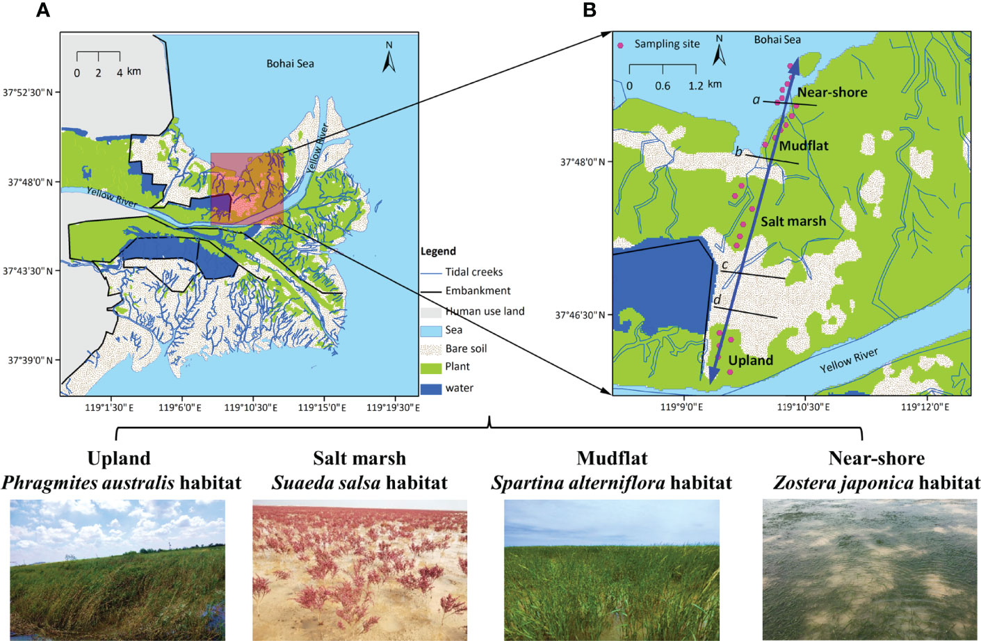
Figure 1 (A) Map of China’s Yellow River Delta based on the interpretation of remote sensing images from 2015. (B) Location of the four studied vegetated habitats along a topographic gradient: Phragmites australis habitat in the upland, Suaeda salsa habitat in the salt marsh, Spartina alterniflora in the mudflat, and Zostera japonica seagrass habitat in the near-shore waters. The black lines represent the approximate borders between adjacent habitats; thus, the lines marked with c and d represent the borders between the marsh and the terrestrial border and between the terrestrial border and the upland habitat, which developed at the highest astronomical tide based on data from Cui et al. (2011) and Li et al. (2020). Photos were taken by X. Li in 2019.

Fieldwork was conducted on the northern shore of the Yellow River channel. There is no tidal embankment along the coastline. Due to the interactions between land and sea, environmental factors vary greatly along the topographic gradient, with the elevation ranging from 0 m at the seashore to 2.5 m at the upland sites; as a result, the flooding frequency ranges from 0% at the upland sites to 95% at the seashore (Cui et al., 2011). The water salinity ranges from <0.5‰ at the upland sites to 30‰ at the seashore (Li et al., 2020). Clear plant zonation patterns are visible along the gradient (Qi et al., 2021). We selected four habitats with different vegetation communities for our study: the P. australis upland, the S. salsa salt marsh, the habitat of invasive S. alterniflora in the mudflat area, and the Z. japonica seagrass habitat in the near-shore waters (Figure 1). In each habitat, we performed sampling at 6 sites (Figure 1B). The macroinvertebrate community also showed large variation across the four habitats, and the dominant macroinvertebrate species changed from insects in the upland habitat to bivalves and gastropods closer to the sea (Li et al., 2020). The large variations in abiotic and biotic factors among the four habitats enable us to further explore the spatial variations in food web characteristics, thereby enriching our understanding of the spatial variation in food web dynamics along the coastal gradient.

Sample Collection and Processing

To determine the spatial variations in food web characteristics across the four vegetated habitats along the coastal topographic gradient, we collected samples of food web items from each habitat in September 2018 and June, July, and August 2019, to cover most of the growing season. We collected potential carbon sources at the base of the food webs, consisting of sediment organic matter (SOM), particulate organic matter (POM), C3 and C4 vascular plants, microphytobenthos, and phytoplankton. We collected zooplankton, macroinvertebrates, and fish to represent consumers in these food webs.

Bulk sediment was collected using a soil core sampler (5.0 cm in diameter, 5.0 cm in depth) to prepare samples of SOM. Water samples were collected at a depth of 20 cm in tidal creeks using a Plexiglass water collector. We filtered the water column through a 200-μm mesh to remove large detritus and then acquired samples of POM by rinsing the samples on pre-combusted (450°C for 6 h) glass-fiber filters (0.45 μm, Whatman GF/F; Mao et al., 2016). We collected fresh leaves of vascular plants by hand and washed them with distilled water. Microphytobenthos samples were collected by scraping the surface of stones in the tidal creek (O’Gorman et al., 2017). Phytoplankton and zooplankton samples were collected by filtration of the collected water column through meshes with sizes of 0.064 and 0.122 mm, respectively. They were then rinsed onto pre-combusted glass-fiber filters for stable isotope determination. Macroinvertebrates were collected by dredging the sediment to a depth of 20 cm. The sediment was then washed and passed through a 0.5-mm mesh to extract organisms. Fish were collected by employing fishing cages in tidal creeks (sampling details see Li et al., 2020).

Different pre-treatments were applied to these organisms before determining the stable isotopic values for carbon (δ¹³C) and nitrogen (δ¹⁵N). For shrimp, we removed the entire shell, head, and tail, and then extracted the muscle tissue. For crabs, we extracted muscle tissue from the large claw. For snails and bivalves, we removed the viscera from the shell. We used the entire body for other small organisms. For fish, we extracted the white dorsal muscle tissues from three individuals per species with similar size or weight to provide a single composite sample for isotope detection. All stable isotope samples were oven-dried at 60°C to constant weight, then ground into a fine powder using a mortar and pestle. Stable isotope analysis was performed in a continuous-flow isotope-ratio mass spectrometer (Delta V Advantage, Thermo Scientific, Schwerte, Germany) coupled with an elemental analyzer (Flash EA1112, Thermo Scientific, Monza, Italy). We recalibrated the spectrometer after every 10 measurements. Measurement precision of δ¹³C and δ¹⁵N were 0.1‰ and 0.2‰, respectively. We used Vienna PeeDee Belemnite (VPDB) and atmospheric N₂, respectively, as the standard samples to calculate the δ¹³C and δ¹⁵N ratios. Since δ¹⁵N ratios change as a result of trophic fractionation, we defined the trophic position (TP) of a consumer trophic group as follows (vander Zanden et al., 1999):

$\begin{array}{ll}TP=[({\text{δ}}^{15}{\text{N}}_{\text{consumer}}{\text{– δ}}^{15}{\text{N}}_{\text{baseline}})/TEF]+2& (1)\end{array}$

where δ¹⁵N_consumer is the consumer’s δ¹⁵N value, and δ¹⁵N_baseline is the baseline δ¹⁵N value, which we assumed equaled the average value for all primary consumers (i.e., detritivores and herbivores) in each habitat. We assumed that the trophic enrichment factors (TEF) were 3.4 ± 1.0‰ (mean ± SD) for δ¹⁵N and 0.4 ± 1.3‰ for δ¹³C, which are the values used in the SIAR model, according to Post (2002). The trophic position of the carbon sources was set to 1.

We divided the collected organisms into different trophic groups, which we defined as groups of taxa that share the same set of prey and predators (Dunne et al., 2002), for each habitat (Supplementary Table 1). In total, we collected 86 stable isotope samples for all trophic groups in the P. australis habitat (Supplementary Table 2), 113 samples in the S. salsa habitat (Supplementary Table 3), 131 samples in the S. alterniflora habitat (Supplementary Table 4), and 117 samples in the Z. japonica habitat (Supplementary Table 5).

Stable Isotope Data Analysis

The size of the region occupied by an assemblage in the stable isotope space (i.e., in the δ¹³C vs. δ¹⁵N plots) contains information about isotopically defined trophic diversity, and reflects the size of the trophic niche (Abrantes et al., 2014). Thus, the close proximity of consumer taxa in isotope space reflects potential trophic redundancy. To investigate differences in trophic niche size of all carbon sources, all consumers combined, and each consumer trophic group among the four habitats, we quantified the value of the corrected standard ellipse area (SEA_c, ‰²) using the SIBER package (Stable Isotope Bayesian Ellipses in R, Jackson et al., 2011) implemented in R version 2.1.6 (https://www.r-project.org/). Higher values of SEA_c indicate wider isotopic trophic niches as well as higher trophic diversity of an assemblage of communities (Masese et al., 2018). For consumers, we further analyzed the percentage overlap of the 95% confidence interval for SEA_c between pairs of habitats. Values of this overlap range from 0% when the two ellipses are completely separated to 100% when they fully overlap. For a target consumer group, a high overlap between pairs of habitats implies that the consumer group relies on similar food sources within the two habitats, which means it has a similar trophic niche in both habitats; conversely, a low overlap means different food sources and trophic niches (Jackson et al., 2011).

We also analyzed the metrics proposed by Layman et al. (2007) to describe the trophic niche structure:

1. δ¹³C range (CR), with a wide range representing niche diversification among carbon sources;

2. δ¹⁵N range (NR), with a wide range suggesting trophic length;

3. total area (TA), which represents the area of the convex hull occupied by the assemblage in the δ¹³C versus δ¹⁵N isotopic space;

4. centroid distance (CD), which represents the Euclidean distance of each component of the species assemblage from the centroid;

5. mean nearest-neighbor distance (MNND), which represents the mean Euclidean distance from each group to its nearest neighbor in the isotopic space;

6. standard deviation of the nearest-neighbor distance (SDNND), which represents the evenness of the isotopic space for all species assemblages.

Lower values of MNND and SDNND indicate higher trophic redundancy; that is, a low MNND means more trophic groups with similar trophic ecologies, and a low SDNND means more evenly distributed species (Abrantes et al., 2014). To overcome the dependence of the six Layman metrics on sample size, we followed the advice of Jackson et al. (2011) and calculated the Bayesian CR, NR, TA, CD, MNND, and SDNND at each habitat using the SIBER package to provide unbiased and more robust metrics that accounted for variations in sample size in our statistical comparisons of the Layman metrics among the four studied habitats.

Bayesian Isotope Mixing Model

We derived the empirical food webs for the four vegetated habitats by combining literature analysis and the Bayesian isotope mixing model. We firstly derived the potential prey for each consumer trophic group in each habitat based on published diet data in similar coastal ecosystems or close to our study area (see Supplementary diet literature). Based on the information on potential food sources, we then ran the Bayesian stable isotope mixing model for each consumer to identify whether the potential feeding link described in the literature was valid at our study sites, and then obtained the quantitative contributions to each consumer’s diet.

We created the Bayesian isotope mixing model using the SIAR package (Stable Isotope Analysis in R; Parnell et al., 2010) implemented in version 3.6.1 of the R software, which solves mixing models based on isotope data using a Markov-chain Monte Carlo approach, and simulates dietary proportions using a Dirichlet prior distribution (Parnell et al., 2010). We ran 30,000 iterations of each SIAR model, and the output represents a probability-density distribution for the potential contribution of each prey item to the diet of each consumer. We assigned a feeding link in the food web when the lower limit of the 50% credibility interval for the contribution of each source to the consumer’s diet exceeded 5% (Careddu et al., 2015; Bentivoglio et al., 2016).

To characterize the trophic structure of food webs across the four habitats along the coastal gradient, we selected 12 commonly addressed topological properties:

1. richness (S), number of trophic groups in the food web;

2. links (L), number of trophic links between the trophic groups;

3. linkage density (LD), LD = L/S;

4. connectance (C), C= L/S²;

5. top species (T), proportion of species that have no predators;

6. intermediate species (I), proportion of species that have both prey and predators;

7. basal species (B), proportion of species that have no prey;

8. omnivory (O), proportion of species that consume prey from more than one trophic level;

9. GenSD, standard deviation of the number of prey resources per species;

10. VulSD, standard deviation of the number of consumers for each species;

11. ATL, average trophic level;

12. MaxSim, maximum Jaccardian similarity.

We calculated these topological properties using the Network 3D software (Yoon et al., 2004; Williams, 2010).

Statistical Analysis

We used one-way ANOVA to identify significant differences in the δ¹³C and δ¹⁵N values of the trophic groups among the four habitats. When the ANOVA test showed a significant difference (p < 0.05), we used Tukey’s HSD post-hoc test to identify significant differences between pairs of habitats. Statistical analyses were conducted using version 20.0 of the Statistical Package for the Social Sciences (SPSS) software (www.ibm.com/analytics/us/en/technology/spss/).

Results

Signatures of Stable Isotope Values of Trophic Groups

δ¹³C and δ¹⁵N Values of Carbon Sources

The δ¹³C values of the carbon sources (i.e., detritus and primary producers) differed significantly among sources in the P. australis habitat (Supplementary Table 2; one-way ANOVA, F_4,40 = 33.54, p < 0.001), the S. salsa habitat (Supplementary Table 3; F_4,43 = 58.23, p < 0.001), the S. alterniflora habitat (Supplementary Table 4; F_4,41 = 51.74, p < 0.001), and the Z. japonica habitat (Supplementary Table 5; F_4,32 = 14.97, p < 0.001). The highest range of mean δ¹³C values of the carbon sources occurred in the S. salsa habitat (from -28.99 ± 0.63‰ to -5.46 ± 0.53‰, mean ± SD), followed by the P. australis habitat (from -25.74 ± 0.67‰ to -6.84 ± 0.75‰), the Z. japonica habitat (from -20.61 ± 3.60‰ to -5.62 ± 0.16‰) and the S. alterniflora habitat (from -19.90 ± 0.02‰ to -7.00 ± 0.79‰) (Figure 2).

FIGURE 2

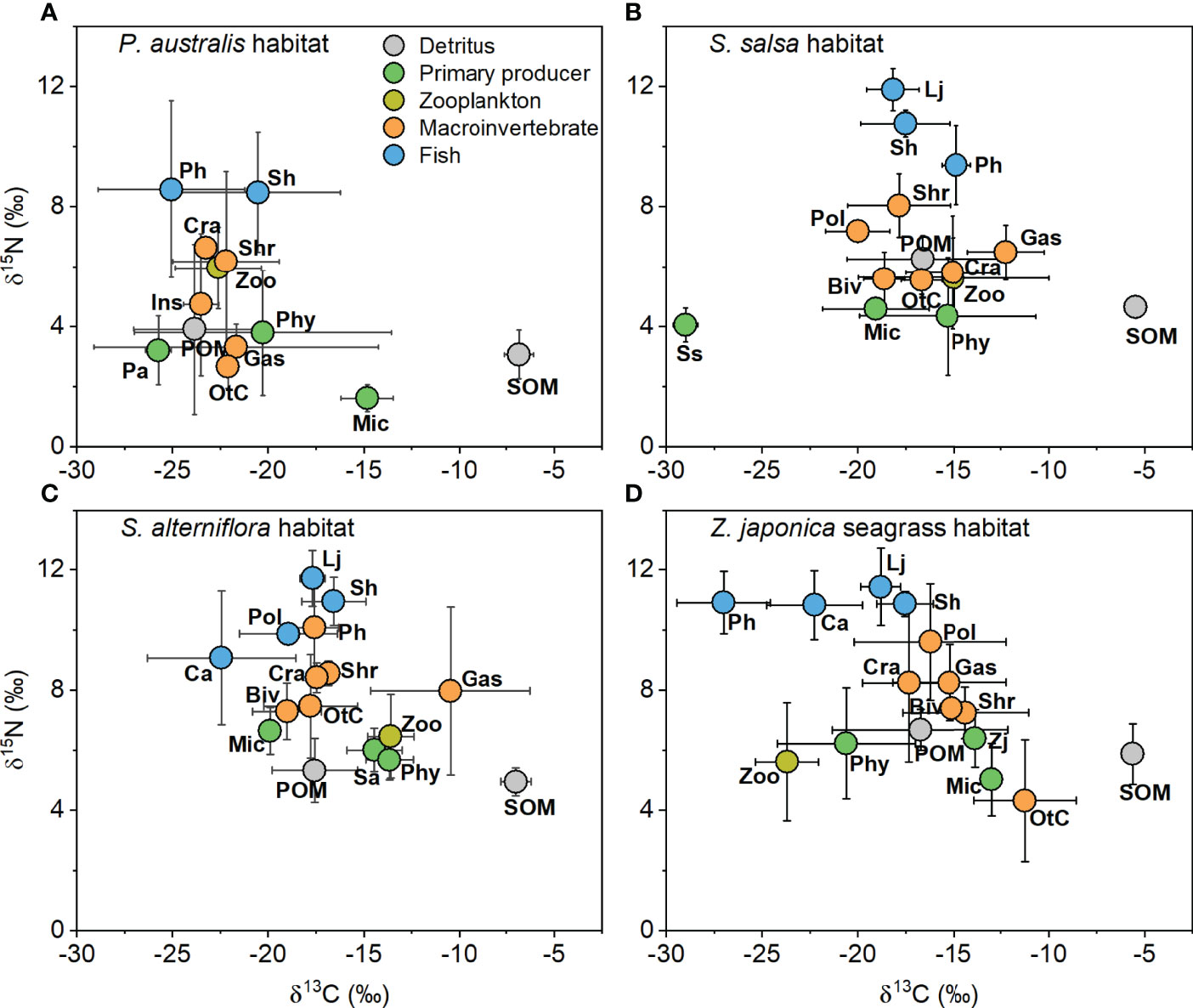
Figure 2 δ¹³C and δ¹⁵N values (mean ± SD) of trophic groups collected from (A) Phragmites australis, (B) Suaeda salsa, (C) Spartina alterniflora, and (D) Zostera japonica seagrass habitats along the coastal topographic gradient in the Yellow River Delta. Abbreviations for the trophic groups: Biv, bivalves; Ca, Carassius auratus; Cra, crabs; Gas, gastropods; Ins, Insects; Lj, Lateolabrax japonicus; Mic, microphytobenthos; OtC, other crustaceans; Pa, Phragmites australis; Ph, Planiliza haematocheila; Phy, phytoplankton; Pol, polychaetes; POM, particulate organic matter; Sa, Spartina alterniflora; Sh, Synechogobius hasta; Shr, shrimp; SOM, sediment organic matter, Ss, Suaeda salsa; Zj, Zostera japonica; Zoo, zooplankton.

In all four habitats, SOM was always the most ¹³C-enriched carbon source (Tukey’s HSD test, p < 0.05, Supplementary Table 2 to 5). In both the P. australis and Z. japonica habitats, phytoplankton (-20.28 ± 6.72‰ and -20.61 ± 3.60‰, respectively) was significantly more ¹³C-depleted than microphytobenthos (-14.82 ± 1.37‰ and -12.97 ± 0.40‰, respectively). In the S. salsa habitat, S. salsa was the most ¹³C-depleted basal source (-28.99 ± 0.63‰), with a value significantly lower than that of other carbon sources (p < 0.05; Supplementary Table 3). In the S. alterniflora habitat, phytoplankton (-13.65 ± 1.25‰) and S. alterniflora (-14.45 ± 1.45‰) were both significantly more ¹³C-enriched than POM (-17.57 ± 2.24‰) and the microphytobenthos (-19.90 ± 0.02‰) (Supplementary Table 4).

The δ¹⁵N values of the carbon sources also showed significant differences in the S. salsa habitat (ANOVA, F_4,43 = 6.37, p < 0.001) and the S. alterniflora habitat (F_4,41 = 3.17, p = 0.02), but there were no significant differences in the P. australis habitat (F_4,40 = 1.54, p = 0.21) and the Z. japonica habitat (F_4,32 = 1.20, p = 0.33). The δ¹⁵N values of the carbon sources ranged from 1.61 ± 0.45‰ to 3.90 ± 2.84‰ in the P. australis habitat, from 4.05 ± 0.56‰ to 6.26 ± 0.78‰ in the S. salsa habitat, from 4.95 ± 0.46‰ to 6.65 ± 0.78‰ in the S. alterniflora habitat, and from 5.02 ± 1.20‰ to 6.68 ± 0.68‰ in the Z. japonica habitat. POM had significantly higher δ¹⁵N values (6.26 ± 0.78‰) than phytoplankton (4.35 ± 1.97‰) in the S. salsa habitat (p < 0.05, Supplementary Table 3).

δ¹³C and δ¹⁵N Values of Consumers

Consumers also showed significant differences in δ¹³C values among the four habitats (for the P. australis habitat, F_7,44 = 3.09, p = 0.01; for the S. salsa habitat, F_9,68 = 3.41, p = 0.002; for the S. alterniflora habitat, F_10,88 = 14.95, p < 0.001; for the Z. japonica habitat, F_10,83 = 17.13, p < 0.001). The distribution of the δ¹³C values of consumers was relatively narrow in the P. australis habitat (from -25.06 ± 4.31‰ to -20.54 ± 3.83‰) compared to the ranges in the S. salsa habitat (from -20.01 ± 1.67‰ to -12.24 ± 2.01‰), the S. alterniflora habitat (from -22.44 ± 3.88‰ to -10.46 ± 4.19‰), and the Z. japonica habitat (from -27.01 ± 2.44‰ to -11.24 ± 2.67‰) (Figure 2 and Supplementary Table 2 to 5). Zooplankton showed more ¹³C-depleted values in the P. australis (-22.61 ± 2.25‰) and Z. japonica (-23.70 ± 1.64‰) habitats than in the S. salsa (-14.99 ± 5.01‰) and S. alterniflora (-13.59 ± 1.21‰) habitats. The macroinvertebrate (mean for all groups ± SD, -22.73 ± 1.85‰) and fish (-23.25 ± 4.35‰) groups both had more ¹³C-depleted values (in average) in the P. australis habitat than in the other habitats: for the S. salsa habitat, -16.20 ± 2.96‰ for macroinvertebrates and -17.66 ± 1.91‰ for fish; for the S. alterniflora habitat, -16.70 ± 3.68‰ for macroinvertebrates and -18.51 ± 3.03‰ for fish; for the Z. japonica habitat, -15.40 ± 3.23‰ for macroinvertebrates and -19.72 ± 3.30‰ for fish. This demonstrates that fish generally had more ¹³C-depleted values than macroinvertebrates in the four habitats.

The consumer δ¹⁵N values also differed significantly (for the P. australis habitat, F_7,44 = 6.16, p < 0.001; for the S. salsa habitat, F_9,68 = 40.24, p < 0.001; for the S. alterniflora habitat, F_10,88 = 10.06, p < 0.001; for the Z. japonica habitat, F_10,83 = 14.93, p < 0.001). In the P. australis habitat, the δ¹⁵N values of other crustaceans (2.66 ± 0.72‰) and gastropods (3.31 ± 0.77‰) were significantly lower than those of the fish (p < 0.001), which were 8.58 ± 2.94‰ and 8.48 ± 1.99‰ for Planiliza haematocheila and Synechogobius hasta, respectively. In the S. salsa, S. alterniflora, and Z. japonica habitats, Lateolabrax japonicus had the highest δ¹⁵N values, and the difference from other groups was often significant. In the S. salsa habitat, P. haematocheila had significantly higher δ¹⁵N values (9.38 ± 1.32‰) than zooplankton (5.63 ± 1.32‰), bivalves (5.59 ± 0.90‰), gastropods (6.48 ± 0.90‰), other crustaceans (5.54 ± 0.47‰), and crabs (5.80 ± 1.89‰) (p < 0.05). In the S. alterniflora habitat, S. hasta had a significantly (p < 0.05) higher δ¹⁵N value (10.95 ± 0.80‰) than zooplankton (6.46 ± 1.39‰), bivalves (7.29 ± 0.94‰), and crabs (7.47 ± 1.71‰). In addition, P. haematocheila, Carassius auratus, and S. hasta in the Z. japonica habitat all had significantly higher δ¹⁵N values than the zooplankton and macroinvertebrates, except for gastropods, crabs, and polychaetes.

Trophic Positions of Consumer Trophic Groups

We determined the trophic positions of consumer trophic groups based on their δ¹⁵N values relative to a baseline that equaled the average value of all detritivores and herbivores for each habitat. The highest trophic position of consumer trophic groups in the S. salsa habitat (3.92) was slightly higher than the highest position in the Z. japonica habitat (3.62), followed by the S. alterniflora (3.32) and P. australis (3.25) habitats (Figure 3). Trophic positions of zooplankton, bivalves, gastropods, C. auratus, S. hasta, and L. japonicus all differed significantly among the four habitats (p < 0.05). Specifically, zooplankton had a higher trophic position in the P. australis habitat (2.41 ± 0.43) than in other habitats, at 1.94 ± 0.42 in the S. salsa habitat, 1.65 ± 0.46 in the S. alterniflora habitat, and 1.76 ± 0.62 for the Z. japonica habitat. In the Z. japonica habitat, bivalves (2.28 ± 0.27), gastropods (2.60 ± 0.40), and C. auratus (3.42 ± 0.37) all had significantly higher trophic positions than in the other habitats (p < 0.05). The trophic positions of S. hasta and L. japonicus were both highest in the S. salsa habitat (3.58 ± 0.14 and 3.94 ± 0.22, respectively), followed by the Z. japonica habitat (3.44 ± 0.13 and 3.62 ± 0.41, respectively), and were lowest in the S. alterniflora habitat (3.08 ± 0.26 and 3.32 ± 0.30, respectively).

FIGURE 3

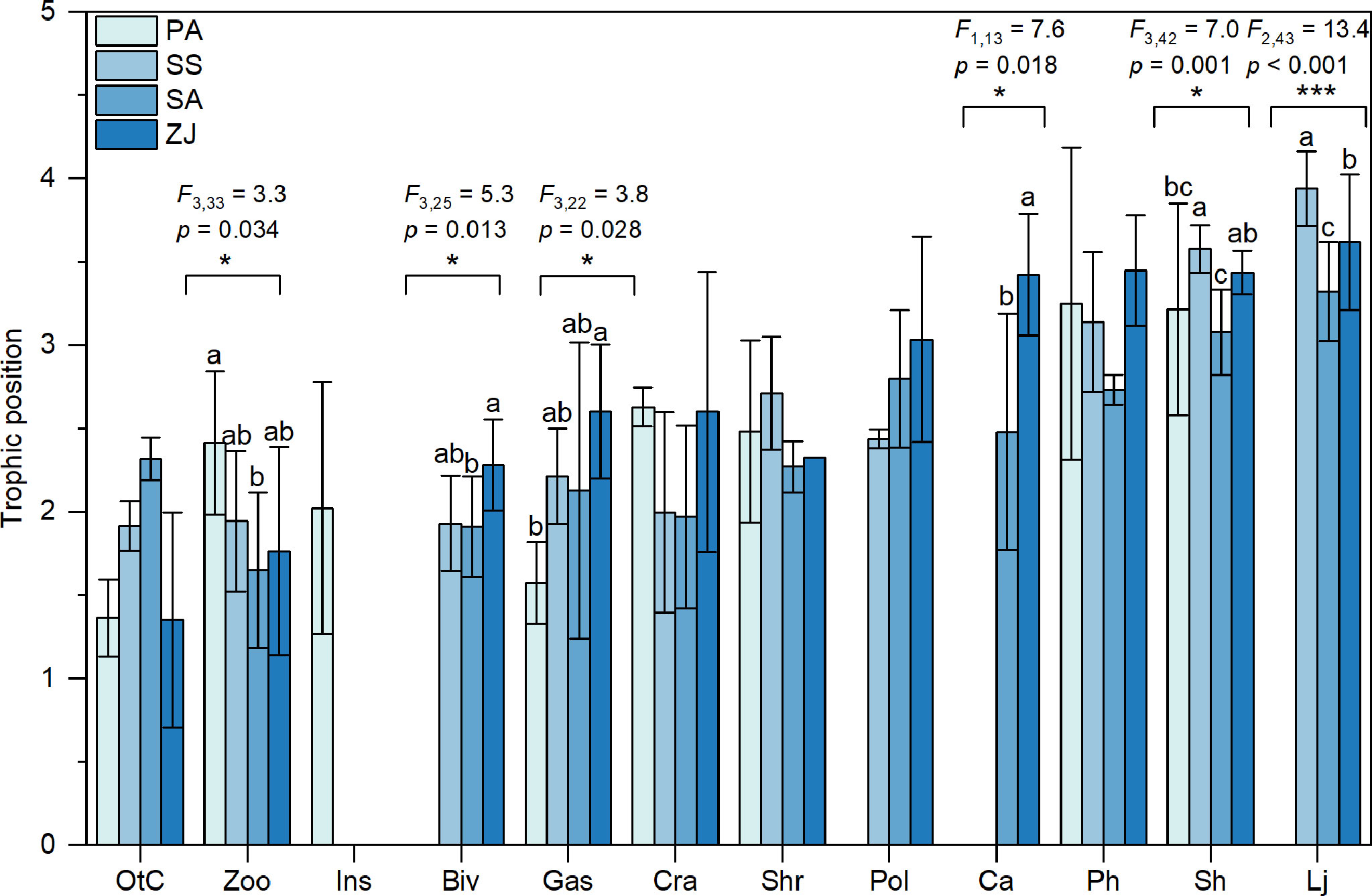
Figure 3 Trophic positions (mean ± SD) identified based on the δ¹⁵N values of consumer trophic groups collected from the Phragmites australis (PA), Suaeda salsa (SS), Spartina alterniflora (SA), and Zostera japonica seagrass (ZJ) habitats along the coastal topographic gradient in the Yellow River Delta wetland. Abbreviations for the trophic groups: Biv, bivalves; Ca, Carassius auratus; Cra, crabs; Gas, gastropods; Ins, Insects; Lj, Lateolabrax japonicus; OtC, other crustaceans; Ph, Planiliza haematocheila; Pol, polychaetes; Sh, Synechogobius hasta; Shr, shrimp; Zoo, zooplankton. The position of consumers on the x-axis from left to right represents an increase in the mean trophic position of the consumers across the four habitats. Significant differences in the trophic positions of the consumers among the four habitats were evaluated by one-way ANOVA (*p < 0.05; ***p < 0.001). Bars for a given trophic group that are labeled with different letters differ significantly (Tukey’s HSD test, p < 0.05).

Trophic Diversity of Trophic Groups

The corrected standard ellipse areas (SEA_c) for different assemblages across the four habitats were calculated by SIBER analysis to identify their relative trophic diversity (Figure 4 and Supplementary Table 6). SEA_c ellipses for the carbon sources, all consumers combined, and individual consumer trophic groups differed among the four habitats in size, shape, and position in the δ¹³C vs. δ¹⁵N plots, which suggested that some trophic groups had shifted their trophic niche along the coastal topographic gradient. In the S. alterniflora and Z. japonica habitats, the positions of the SEA_c ellipses for the carbon sources, all consumers combined, gastropods, and S. hasta showed higher δ¹³C and δ¹⁵N values than in the P. australis and S. salsa habitats (Figures 4A, B, E, I). In addition, the SEA_c of bivalves and crabs showed higher δ¹⁵N values in the S. alterniflora and Z. japonica habitats than in the S. salsa habitat (Figures 4D, F).

FIGURE 4

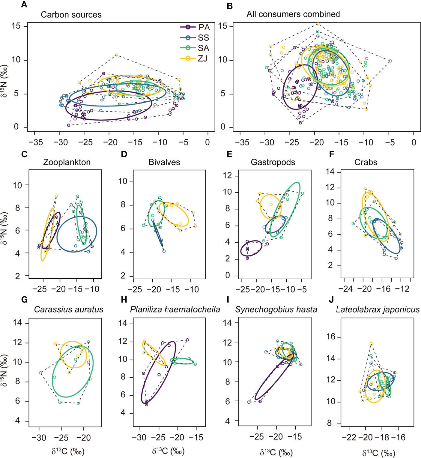
Figure 4 Corrected standard niche ellipses (solid lines) and convex hulls (dashed lines) for the isotope-based niche areas of (A) the carbon sources, consisting of detritus and primary producers; (B) all consumers combined; and (C-J) individual consumer trophic groups for the Phragmites australis (PA), Suaeda salsa (SS), Spartina alterniflora (SA), and seagrass Zostera japonica seagrass (ZJ) habitats along the coastal topographic gradient in the Yellow River Delta wetland. Graphs were produced using the SIBER package implemented in the R software. Each point shows the δ¹³C and δ¹⁵N values for a sample, with colors based on the habitat where this data was collected. The ellipses, hulls, and data points for a given consumer trophic group collected in a given habitat in (C) to (J) are only provided when the sample size is ≥ 5.

Regarding the size of SEA_c, S. alterniflora habitat had the smallest SEA_c for both carbon sources (11.32‰²) and all consumers combined (25.86‰²) (Figure 4 and Supplementary Table 6). Specifically, for zooplankton, SEA_c was largest in the S. salsa habitat (22.51‰²) and smallest in the S. alterniflora habitat (4.91‰²). Bivalves and crabs gradually had larger SEA_c from the S. salsa habitat to the S. alterniflora and Z. japonica habitats. Gastropods had the largest SEA_c in the S. alterniflora (27.41‰²), followed by the Z. japonica habitat (13.62‰²), with lower values in the P. australis and S. salsa habitats (< 9‰²). P. haematocheila and S. hasta both had the largest SEA_c in the P. australis habitat (22.90‰² and 10.41‰², respectively), whereas C. auratus had the largest SEA_c in the S. alterniflora habitat (29.08‰²). Variation of SEA_c of L. japonicus among the four habitats was small, with values ranging from 1.53‰² to 4.47‰².

Supplementary Table 7 summarizes the overlaps of the ellipses among the four sites. Trophic groups showed high overlaps among the four habitats (Figure 4), with overlaps ranging from 24.5% to 60.0% for the carbon sources, and from 27.7 to 81.5% for all consumers combined. In addition, only the overlaps for zooplankton between the P. australis and S. alterniflora habitats and for bivalves between the S. salsa and Z. japonica habitats were lower than 6%.

Layman’s community metrics also varied across habitats, but with strongly different patterns (Figure 5). CR, TA, and CD showed similar patterns across the four habitats, with their highest values in the S. salsa habitat, followed by the P. australis or Z. japonica habitat, and the lowest values in the S. alterniflora habitat. This contrasts with the NR metric, which was lowest in the S. salsa habitat and highest in the S. alterniflora habitat. MNND was highest in the S. salsa habitat, followed by the P. australis and S. alterniflora habitats, but lowest in the Z. japonica habitat. Whereas SDNND was highest in the Z. japonica habitat, followed by the S. salsa habitat, and lowest in the P. australis habitat.

FIGURE 5

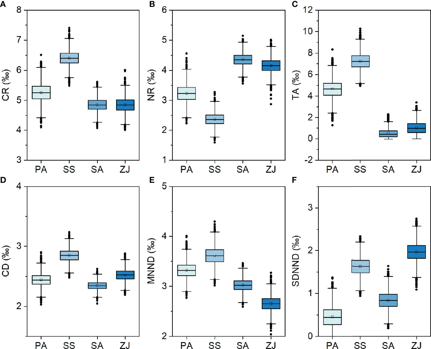
Figure 5 Boxplots representing Bayesian model estimates for six Layman community metrics: (A) the δ¹³C range (CR), (B) the δ¹⁵N range (NR), (C) the total area (TA), (D) the mean distance to the centroid (CD), (E) the mean nearest-neighbor distance (MNND), and (F) the standard deviation of the nearest-neighbor distance (SDNND) across the Phragmites australis (PA), Suaeda salsa (SS), Spartina alterniflora (SA), and Zostera japonica seagrass (ZJ) habitats along the coastal topographic gradient in the Yellow River Delta wetland.

Food Web Trophic Structure and Topological Properties

The SIAR modeling revealed high variability in the diet compositions of the consumer trophic groups across the four habitats (Figure 6), except for insects, shrimps, and polychaetes. Diagrams of the trophic structure of these food webs were shown in Supplementary Figures 1–4. The diet composition of zooplankton was relatively evenly distributed in the P. australis and Z. japonica habitats, with POM and phytoplankton accounting for 60% and 40% in the P. australis habitat, and 54% and 46% in the Z. japonica habitat, respectively. Whereas zooplankton relied almost exclusively on phytoplankton (ca. 83%) in both the S. salsa and S. alterniflora habitats. Bivalves showed a slight dietary preference for phytoplankton (61%) in the S. salsa habitat, but depended on POM (59%) in the Z. japonica habitat. Bivalves had a particularly high preference for POM (89%) in the S. alterniflora habitat. Gastropods had relatively evenly distributed diet compositions, with the highest contribution by P. australis (37%) in the P. australis habitat. In the other three habitats, gastropods mostly relied on SOM (53, 47, and 44% for the S. salsa, S. alterniflora, and Z. japonica habitats, respectively), followed by S. alterniflora (32%) in the S. alterniflora habitat and microphytobenthos in the S. salsa and Z. japonica habitats (ca. 30%). A range of prey contributed to the diet of crabs in these four habitats, with the highest contribution of 24% from P. australis in the P. australis habitat, ca. 19% from SOM in the S. salsa and Z. japonica habitats, and 24% from POM in the S. alterniflora habitat. Large differences were evident in the dietary composition of the other crustaceans across the four habitats; they relied substantially on POM in the P. australis habitat (85%) and S. alterniflora habitat (63%), but only approximately 50% on both SOM and POM in the S. salsa and Z. japonica habitats.

FIGURE 6

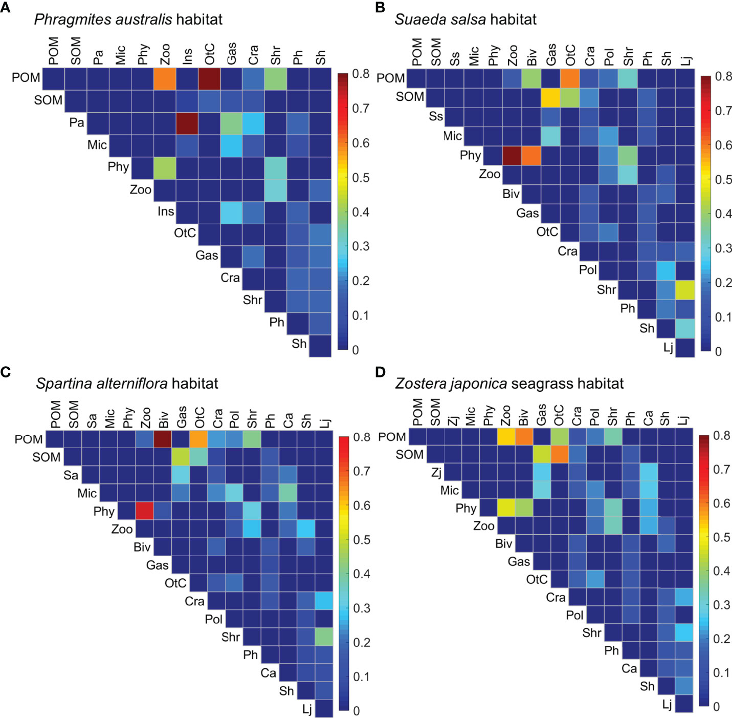
Figure 6 Diet compositions for each trophic group (in the columns) foraging on its prey (in the rows) in the (A) Phragmites australis, (B) Suaeda salsa, (C) Spartina alterniflora, and (D) Zostera japonica seagrass habitats along the coastal topographic gradient in the Yellow River Delta wetland. Color intensity is proportional to the magnitude of the diet contributions of the prey to the consumer trophic groups. Abbreviations for the trophic groups: Abbreviations for the trophic groups: Biv, bivalves; Ca, Carassius auratus; Cra, crabs; Gas, gastropods; Ins, Insects; Lj, Lateolabrax japonicus; Mic, microphytobenthos; OtC, other crustaceans; Pa, Phragmites australis; Ph, Planiliza haematocheila; Phy, phytoplankton; Pol, polychaetes; POM, particulate organic matter; Sa, Spartina alterniflora; Sh, Synechogobius hasta; Shr, shrimp; SOM, sediment organic matter, Ss, Suaeda salsa; Zj, Zostera japonica; Zoo, zooplankton.

The fish P. haematocheila, C. auratus, and S. hasta all had broad diet compositions, with no dominant prey. However, microphytobenthos accounted for 38% of the diet of C. auratus, and S. hasta preferred polychaetes and shrimp in the S. salsa habitat but zooplankton and crabs in the S. alterniflora habitat. L. japonicus had obvious diet preferences across these habitats; it preferred shrimps (46%) and S. hasta (30%) in the S. salsa habitat, shrimps (41%) and crabs (27%) in the S. alterniflora habitat, and all three prey (ranging from 20 to 26%) in the Z. japonica habitat.

We observed clear differences among the four habitats in the food web topological properties (Table 1). S, L, LD, I, and O were all higher in the S. alterniflora and Z. japonica habitats than in the S. salsa habitat, and were lowest in the P. australis habitat. In contrast, C, T, B, and MaxSim showed the opposite pattern, though the differences were very small.

TABLE 1

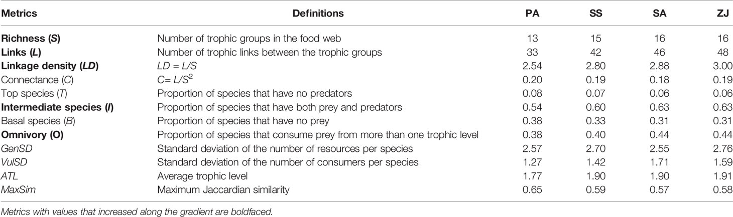
Table 1 Topological properties of the food webs in the Phragmites australis (PA), Suaeda salsa (SS), Spartina alterniflora (SA), and Zostera japonica seagrass (ZJ) habitats along the coastal topographic gradient in the Yellow River Delta.

Discussion

Despite the challenges in resolving empirical coastal food webs on a large scale, this study disentangled the spatial variation of the trophic diversity of trophic groups and the structure of the entire food web across variable vegetated habitats along a coastal topographic gradient in the Yellow River Delta. Our two initial hypotheses were both confirmed. Specifically, the measured stable isotope ratios of the trophic groups, the trophic positions of consumers, the isotopically defined trophic diversity, the quantitative diet compositions, and the topological properties all varied markedly along the coastal topographic gradient. However, we found no consistent trend for multiple metrics of trophic diversity and trophic structure. It is worth noting that trophic groups in the habitat dominated by invasive S. alterniflora mostly had rather low values of isotopically defined trophic diversity. The seaside habitats had higher values of food web topological properties than the higher-elevation habitats in terms of species richness, number of trophic links, and linkage density; that is, they had more complex food webs.

Spatial Variability in Trophic Diversity of the Trophic Groups Along the Topographic Gradient

Our measured δ¹³C values for the carbon sources in the four habitats were similar to those that were previously reported for temperate estuarine and coastal ecosystems in other parts of the world (Bristow et al., 2013; Park et al., 2017; Kim et al., 2020). However, our δ¹³C value for Z. japonica seagrass (-13.8 ± 0.3‰) was slightly lower than that for the same species along the Gudong embankment in the Yellow River Delta’s coastal wetland (-11.7 ± 0.4‰) (Li et al., 2021) and lower than the range in a review of 31 studies in seagrass ecosystems (-10 to -11‰) (Hemminga and Mateo, 1996), but approached the values (-10.1 to 14.0‰) in some temperate seagrass beds (e.g., Hanson et al., 2010; Mittermayr et al., 2014). We found that the C4 plants of S. alterniflora and Z. japonica seagrass were significantly more ¹³C-enriched than the C3 plants of P. australis and S. salsa, probably due to their different photosynthetic pathways (Peterson and Fry, 1987). SOM was more ¹³C-enriched than POM in all four habitats, which is consistent with a previously reported separation between pelagic and benthic carbon sources (Kiljunen et al., 2020). However, our comparisons between pelagic algae (i.e., phytoplankton) and benthic algae (i.e., microphytobenthos) tended to be confused among the four habitats. That is, phytoplankton were more ¹³C-depleted than microphytobenthos in both P. australis and Z. japonica habitats, but less ¹³C-depleted in the S. salsa and S. alterniflora habitats.

The phytoplankton δ¹³C values (ca. -15‰) in the S. salsa and S. alterniflora habitats were lower than the values commonly observed in temperate waters (-22 to -20‰; Cresson et al., 2012). We hypothesize that our conservative estimates for the phytoplankton stable isotope signatures in the two habitats were either influenced by water salinity and dissolved inorganic carbon (Careddu et al., 2015) or due to the fact that the collected phytoplankton may reflect a combination of phytoplankton, microorganisms, and POM of undefined origins (Young et al., 2021). The lower δ¹³C values for SOM in the higher-elevation P. australis habitat compared with the lower-elevation S. alterniflora and Z. japonica habitats are consistent with the findings of Park et al. (2017), and are also consistent with observations that the δ¹³C values of POM in freshwater are significantly lower than those in saltwater (Dibble and Meyerson, 2014; Ye et al., 2017). The microphytobenthos δ¹³C values in the P. australis and Z. japonica habitats (ca. -15‰) were slightly higher than those in the S. salsa and Z. japonica habitats (ca. -19‰), but were comparable with the range (-14.8 ± 0.8‰) reported in coastal wetlands (Kim et al., 2020).

The overall δ¹³C range of the consumers collected from the P. australis habitat was narrow and the values were lower than those in the other three habitats, possibly reflecting the carbon isotopic signatures of the dominant primary producer (Wozniak et al., 2006). Similarly, Park et al. (2015) showed that the δ¹³C values of consumers in P. australis habitat were lower than those in the Suaeda japonica habitat. Garcia et al. (2018) showed an overall increasing trend in mean consumer δ¹³C values along a river–estuary–surf zone transect. Higher consumer δ¹⁵N values were found in the seaside habitats (i.e., the S. salsa, S. alterniflora, and Z. japonica habitats) than in the P. australis habitat, which is in line with the findings of Kim et al. (2020). The highest trophic position for all consumers combined was observed in the S. salsa habitat, followed by the Z. japonica habitat, and was lower in the S. alterniflora and P. australis habitats. The trophic positions are comparable to the value (3.76) for the highest trophic position reported in the lower reaches of the Yangtze River (Mao et al., 2016). We found the highest trophic position for the sea bass, L. japonicus, in the S. salsa, S. alterniflora, and Z. japonica habitats, which is consistent with recent studies showing that L. japonicus is a typical top predator in China’s coastal and offshore waters (Islam et al., 2011; Li et al., 2021). It is worth noting that the four fish species, as well as the zooplankton, bivalves, crabs, and shrimps, had the lowest average trophic positions in the habitat dominated by the invasive S. alterniflora habitat. Thus, we hypothesize that S. alterniflora, despite its dense distribution pattern and high biomass, transferred less primary productivity to higher trophic levels. This is might because consumers rarely ingest S. alterniflora directly (Wittyngham, 2021). In addition, S. alterniflora detritus is largely buried in sediments as plant-derived carbon affected by the decomposition of microorganisms or washed to adjacent coasts due to tidal dynamics, which both imply that its production is rarely recycled to higher trophic levels (Yan et al., 2019; Zhang et al., 2021).

Based on the trophic diversity revealed by the SIBER analysis, the habitat dominated by invasive S. alterniflora showed weak ecosystem functioning, as it had the lowest SEA_c, CR, TA, and CD values for carbon sources and for all consumers combined. This suggests that there was a low separation in δ¹³C values among carbon sources in the habitat, and that consumers tended to have similar niche signatures (Abrantes et al., 2014). Similarly, Feng et al. (2018) found that communities in S. alterniflora habitat had lower SEA_c than natural mangrove forests, indicating significant resource competition among different consumers in the S. alterniflora habitat.

We observed a large overlap among the ellipses for all consumers combined in the S. salsa, S. alterniflora, and Z. japonica habitats, indicating high competition in resource utilization among consumers in the three habitats. In contrast, consumers in these three habitats overlapped less with the P. australis habitat, suggesting a large habitat heterogeneity between the P. australis habitat and the three habitats. This is probably mainly due to the composition of the macroinvertebrate consumers, which were dominated by insects in the P. australis habitat, but were dominated by bivalves, gastropods, and polychaetes in the S. salsa, S. alterniflora, Z. japonica habitats due to their living habits in brackish water and saltwater (Dauer et al., 2010; Li et al., 2020).

Habitat Heterogeneity Created Highly Variable Food Webs Along the Topographic Gradient

Though insects, shrimps, and polychaetes showed little variation across the four habitats, other consumers and the overall food web trophic structure displayed high variation based on the SIAR analysis. Zooplankton showed a much higher reliance on phytoplankton in the S. alterniflora and Z. japonica habitats than in the P. australis and S. salsa habitats, indicating that the S. alterniflora and Z. japonica habitats are strongly influenced by nutrition imports from the adjacent marine ecosystem (Heck et al., 2008). Bivalves, as typical filter-feeding organisms, showed dietary preferences for POM and phytoplankton, which is consistent with previous studies (Atkinson et al., 2014; Li et al., 2021). Gastropods showed a slight preference for direct feeding on P. australis, S. salsa, and seagrass, but ca. 32% of the diet was S. alterniflora. Similarly, Feng et al. (2014) found that gastropods in a Spartina wetland derived more than 80% of their organic carbon from Spartina. In agreement with previous studies (Evrard et al., 2012; Kim et al., 2020), we also found that gastropods relied greatly on SOM and the microphytobenthos. Unfortunately, we did not sample epiphytes attached to plant leaves, which have been determined to be one of the main energy providers to gastropods, especially in seagrass meadows (Cook et al., 2011; Voigt and Hovel, 2019). Crabs showed highly generalist feeding in the Yellow River Delta coastal wetland, as they fed on both pelagic and benthic carbon sources, as well as on detritus and primary producers. Together with their high abundance in coastal wetlands, crabs are a key component of coastal food webs, and their trophic interactions play a fundamental role in maintaining food web stability (Vermeiren et al., 2015; Hoy et al., 2019).

Since we defined a trophic group as a species cluster that shares the same prey and predators, we considered less complex food webs than in some previous studies conducted in estuarine and coastal wetlands (Vinagre and Costa, 2014; Careddu et al., 2015; Mendonça et al., 2018). Despite the small variation in the number of trophic groups, we found that other topological properties differed along the topographic gradient. The linkage density values of the four habitats (2.54 to 3.00) were lower than previously reported values (ca. 2.5 to 3.8) in an estuary–coastal system (Vinagre and Costa, 2014) and some other aquatic ecosystems (Mor et al., 2018; Kortsch et al., 2019), but fell with the range (1.6 to 25.1) for empirical food webs reported by Dunne et al. (2002). We found that our seaside habitats had higher values of the topological metrics than the higher-elevation habitats, similarly, Vinagre and Costa (2014) found upper estuary had the lowest values of linkage density than habitats in the lower estuary. The proportion of omnivorous consumers in our study ranged from 38 to 44%, which was much higher than the values (11 to 20%) reported in a riverine ecosystem (Mor et al., 2018) and (11 to 39%) in intertidal pools (Mendonça et al., 2018), but lower than the reported range (45 to 65%) for estuarine wetlands (Vinagre and Costa, 2014).

Implications for Coastal Wetland Conservation and Management

Recent research on food web changes along a coastal topographic gradient has been scarce (e.g., Robson et al., 2017) compared to the number conducted along variable environmental gradients in riverine ecosystems (Mor et al., 2018), lacustrine ecosystems (van der Lee et al., 2021), and marine ecosystems (Kortsch et al., 2015; Nordström and Bonsdorff, 2017). This is an important research gap, since coastal wetlands display significant variations in environmental factors and biological signatures such as the community composition, species stress tolerance, and trophic niche width. Thus, the heterogeneous habitats should create highly variable food web characteristics along coastal environmental or geographic gradients, which agrees with the results of our study. With the intensification of human coastal activities such as seashore reclamation, ditch diversion, and aquaculture, the habitat heterogeneity of coastal wetland has been both, directly and indirectly, decreased, leading to a decrease in species taxonomic and functional diversity, and ultimately resulting in a more homogeneous ecosystem with relatively similar food web attributes (Feit et al., 2019; Li et al., 2019). This will ultimately pose a major threat to biodiversity conservation, ecosystem functions, and the maintenance of ecosystem resilience (Thrush et al., 2008; Lohrer et al., 2015).

The invasive species S. alterniflora showed relatively weak ecosystem functions compared with the adjacent communities of native S. salsa and seagrass, especially in terms of the trophic positions of consumers and the isotopically defined trophic diversity. This suggests that S. alterniflora wetland has not formed a healthy ecosystem and has not effectively performed ecosystem functioning, even though the invasion began about 10 years before our study. Given the rapid expansion of this species, with its area increasing by 50,204 ha during the past 25 years along the Chinese coastline (Mao et al., 2019), our results suggest that more protective measures should be taken to limit its spread and thereby protect or enhance the function of coastal ecosystems. Recently, many studies have tried to identify the effects of the invasion by S. alterniflora to better control and remove the species (Ainouche and Gray, 2016; Meng et al., 2020). Unfortunately, managing this species at an ecosystem scale has proven difficult (Wails et al., 2021). Further studies will be needed to investigate how ecosystem functions such as energy transfer efficiency and ecosystem stability are affected by the S. alterniflora invasion. The results should provide new insights that will lead to the development of more effective management strategies with practical and attainable goals.

Conclusions

In this study, we combined the isotopically defined trophic diversity from the SIBER analysis with the quantitative trophic structure from the SIAR analysis to investigate the spatial variation of empirically resolved food webs across variable vegetated habitats along a coastal topographic gradient. Although we didn’t reveal a continuous overall trend for changes in the food web characteristics due to inconsistent trends for different metrics of trophic diversity and structure, we nonetheless observed that the δ¹³C values of the carbon sources and the δ¹⁵N values of the consumers were both higher in the seaside habitats than in the higher-elevation habitats. The habitat dominated by invasive S. alterniflora had the lowest values for most metrics in the SIBER analysis, indicating weak ecosystem functioning in terms of the trophic niche characteristics. The relative diet contributions for the consumers varied greatly among the four habitats, except for shrimps and polychaetes. The complexity of the food webs increased along the gradient from upland to near-shore habitats in terms of the species richness, the number of trophic links, and the linkage density. In addition, the proportions of intermediate consumers and omnivores and the average trophic level also increased along this gradient. Overall, we found that habitat heterogeneity formed highly variable food webs along the topographic gradient. This knowledge will enhance our ability to protect the coastal habitat heterogeneity, which plays a decisive role in maintaining biodiversity and ecosystem functions. Based on our results, we propose that more attention should be paid to the habitat dominated by invasive S. alterniflora in China’s coastal wetlands, and that adaptive and effective management should be implemented at an ecosystem scale to mitigate the impacts of this invasion.

Data Availability Statement

The original contributions presented in the study are included in the article/supplementary material. Further inquiries can be directed to the corresponding authors.

Author Contributions

XL and WY conceived the original idea and designed the study. XL performed the field sampling and data analysis under the joint supervision of WY, TS, and ZY. XL wrote the first draft of the manuscript. All authors contributed to manuscript revision, and have read and approved the manuscript for submission.

Funding

This study was financially supported by the Joint Funds of the National Natural Science Foundation of China (U1806217), the Program for Guangdong Introducing Innovative and Entrepreneurial Teams (2019ZT08L213), the Key Special Project for Introduced Talents Team of Southern Marine Science and Engineering Guangdong Laboratory (Guangzhou) (GML2019ZD0403), and the Guangdong Provincial Key Laboratory Project (2019B121203011).

Conflict of Interest

The authors declare that the research was conducted in the absence of any commercial or financial relationships that could be construed as a potential conflict of interest.

Publisher’s Note

All claims expressed in this article are solely those of the authors and do not necessarily represent those of their affiliated organizations, or those of the publisher, the editors and the reviewers. Any product that may be evaluated in this article, or claim that may be made by its manufacturer, is not guaranteed or endorsed by the publisher.

Acknowledgments

We are indebted to Jun Pei, Ziyue Zhang, and Xianting Fu for invaluable field assistance. We also thank Geoffrey Hart for providing language help during the writing of this paper.

Supplementary Material

The Supplementary Material for this article can be found online at: https://www.frontiersin.org/articles/10.3389/fmars.2022.920745/full#supplementary-material

References

Abrantes K. G., Barnett A., Bouillon S. (2014). Stable Isotope-Based Community Metrics as a Tool to Identify Patterns in Food Web Structure in East African Estuaries. Funct. Ecol. 28 (1), 270–282. doi: 10.1111/1365-2435.12155

CrossRef Full Text | Google Scholar

Ainouche M., Gray A. (2016). Invasive Spartina: Lessons and Challenges. Biol. Invas. 18 (8), 2119–2122. doi: 10.1007/s10530-016-1201-7

CrossRef Full Text | Google Scholar

Atkinson C. L., Kelly J. F., Vaughn C. C. (2014). Tracing Consumer-Derived Nitrogen in Riverine Food Webs. Ecosystems 17, 485–496. doi: 10.1007/s10021-013-9736-2

CrossRef Full Text | Google Scholar

Baiser B., Gravel D., Cirtwill A. R., Dunne J. A., Fahimipour A. K., Gilarranz L. J., et al. (2019). Ecogeographical Rules and the Macroecology of Food Webs. Global Ecol. Biogeogr. 28, 1204–1218. doi: 10.1111/geb.12925

CrossRef Full Text | Google Scholar

Baker R., Abrantes K., Feller I. C. (2021). Stable Isotopes Suggest Limited Role of Wetland Macrophyte Production Supporting Aquatic Food Webs Across a Mangrove-Salt Marsh Ecotone. Estuar. Coast. 44, 1619–1627. doi: 10.1007/s12237-021-00895-5

CrossRef Full Text | Google Scholar

Bang J. H., Bae M. J., Lee E. J. (2018). Plant Distribution Along an Elevational Gradient in a Macrotidal Salt Marsh on the West Coast of Korea. Aquat. Bot. 147, 52–60. doi: 10.1016/j.aquabot.2018.03.005

CrossRef Full Text | Google Scholar

Barbier E. B., Hacker S. D., Kennedy C., Koch E. W., Stier A. C., Silliman S. B. R. (2011). The Value of Estuarine and Coastal Ecosystem Services. Ecol. Monogr. 81, 169–193. doi: 10.1890/10-1510.1

CrossRef Full Text | Google Scholar

Bentivoglio F., Calizza E., Rossi D., Carlino P., Careddu G., Rossi L., et al. (2016). Site-Scale Isotopic Variations Along a River Course Help Localize Drainage Basin Influence on River Food Webs. Hydrobiologia 770, 257–272. doi: 10.1007/s10750-015-2597-2

CrossRef Full Text | Google Scholar

Bristow L. A., Jickells T. D., Weston K., Marca-Bell A., Parker R., Andrews J. E. (2013). Tracing Estuarine Organic Matter Sources Into the Southern North Sea Using C and N Isotopic Signatures. Biogeochemistry 113, 9–22. doi: 10.1007/s10533-012-9758-4

CrossRef Full Text | Google Scholar

Cardona L., Lloret-Lloret E., Moles J., Avila C. (2021). Latitudinal Changes in the Trophic Structure of Benthic Coastal Food Webs Along the Antarctic Peninsula. Mar. Environ. Res. 167, 105290. doi: 10.1016/j.marenvres.2021.105290

PubMed Abstract | CrossRef Full Text | Google Scholar

Careddu G., Costantini M. L., Calizza E., Carlino P., Bentivoglio F., Orlandi L., et al. (2015). Effects of Terrestrial Input on Macrobenthic Food Webs of Coastal Sea are Detected by Stable Isotope Analysis in Gaeta Gulf. Estuar. Coast. Shelf. Sci. 154, 158–168. doi: 10.1016/j.ecss.2015.01.013

CrossRef Full Text | Google Scholar

Christianen M. J. A., Middelburg J. J., Holthuijsen S. J., Jouta J., Compton T. J., van der Heide T., et al. (2017). Benthic Primary Producers are Key to Sustain the Wadden Sea Food Web: Stable Carbon Isotope Analysis at Landscape Scale. Ecology 98, 1498–1512. doi: 10.1002/ecy.1837

PubMed Abstract | CrossRef Full Text | Google Scholar

Colombano D. D., Litvin S. Y., Ziegler S. L., Alford S. B., Baker R., Barbeau M. A., et al. (2021). Climate Change Implications for Tidal Marshes and Food Web Linkages to Estuarine and Coastal Nekton. Estuar. Coast. 44, 1637–1648. doi: 10.1007/s12237-020-00891-1

CrossRef Full Text | Google Scholar

Cook K., Vanderklift M. A., Poore A. G. B. (2011). Strong Effects of Herbivorous Amphipods on Epiphyte Biomass in a Temperate Seagrass Meadow. Mar. Ecol. Progr. Ser. 442, 263–269. doi: 10.3354/meps09446

CrossRef Full Text | Google Scholar

Cresson P., Ruitton S., Fontaine M. F., Harmelin-Vivien M. (2012). Spatio-Temporal Variation of Suspended and Sedimentary Organic Matter Quality in the Bay of Marseilles (NW Mediterranean) Assessed by Biochemical and Isotopic Analyses. Mar. Pollut. Bull. 64 (6), 1112–1121. doi: 10.1016/j.marpolbul.2012.04.003

PubMed Abstract | CrossRef Full Text | Google Scholar

Cui B. S., He Q., An Y. (2011). Community Structure and Abiotic Determinants of Salt Marsh Plant Zonation Vary Across Topographic Gradients. Estuar. Coast. 34, 459–469. doi: 10.1007/s12237-010-9364-4

CrossRef Full Text | Google Scholar

Dauer D. M., Ewing R. M., Rodi A. J. Jr. (2010). Macrobenthic Distribution Within the Sediment Along an Estuarine Salinity Gradient. Internat. Rev. Hydrobiol. 72, 529–538. doi: 10.1002/iroh.19870720502

CrossRef Full Text | Google Scholar

Dibble K. L., Meyerson L. A. (2014). The Effects of Plant Invasion and Ecosystem Restoration on Energy Flow Through Salt Marsh Food Webs. Estuar. Coast. 37, 339–353. doi: 10.1007/s12237-013-9673-5

CrossRef Full Text | Google Scholar

Dunne J. A., Williams R. J., Martinez N. D. (2002). Food-Web Structure and Network Theory: The Role of Connectance and Size. Proc. Natl. Acad. Sci. U.S.A. 99, 12917–12922. doi: 10.1073/pnas.192407699

PubMed Abstract | CrossRef Full Text | Google Scholar

Engels J. G., Rink F., Jensen K. (2011). Stress Tolerance and Biotic Interactions Determine Plant Zonation Patterns in Estuarine Marshes During Seedling Emergence and Early Establishment. J. Ecol. 99, 277–287. doi: 10.1111/j.1365-2745.2010.01745.x

CrossRef Full Text | Google Scholar

Evrard V., Huettel M., Cook P. L. M., Soetart K., Middelburg J. J. (2012). Importance of Phytodetritus and Microphytobenthos for Heterotrophs in a Shallow Subtidal Sandy Sediment. Mar. Ecol. Progr. Ser. 455, 13–31. doi: 10.3354/meps09676

CrossRef Full Text | Google Scholar

Feit B., Blüthgen N., Traugott M., Jonsson M. (2019). Resilience of Ecosystem Processes: A New Approach Shows That Functional Redundancy of Biological Control Services is Reduced by Landscape Simplification. Ecol. Lett. 22, 1568–1577. doi: 10.1111/ele.13347

PubMed Abstract | CrossRef Full Text | Google Scholar

Feng J. X., Guo J. M., Huang Q., Jiang J. X., Huang G. M., Yang Z. W., et al. (2014). Changes in the Community Structure and Diet of Benthic Macrofauna in Invasive Spartina Alterniflora Wetlands Following Restoration With Native Mangroves. Wetlands 34, 673–683. doi: 10.1007/s13157-014-0533-2

CrossRef Full Text | Google Scholar

Feng J. X., Huang Q., Chen H., Guo J. M., Lin G. H. (2018). Restoration of Native Mangrove Wetlands can Reverse Diet Shifts of Benthic Macrofauna Caused by Invasive Cordgrass. J. Appl. Ecol. 55 (2), 905–916. doi: 10.1111/1365-2664.12987

CrossRef Full Text | Google Scholar

Garcia A. F. S., Santos M. L., Garcia A. M., Vieira J. P. (2018). Changes in Food Web Structure of Fish Assemblages Along a River-to-Ocean Transect of a Coastal Subtropical System. Mar. Freshwat. Res. 70, 402–416. doi: 10.1071/MF18212

CrossRef Full Text | Google Scholar

Hanson C. E., Hyndes G. A., Wang S. F. (2010). Differentiation of Benthic Marine Primary Producers Using Stable Isotopes and Fatty Acids: Implications to Food Web Studies. Aquat. Bot. 93 (2), 114–122. doi: 10.1016/j.aquabot.2010.04.004

CrossRef Full Text | Google Scholar

Heck K. L. Jr., Carruthers T. J. B., Duarte C. M., Hughes A. R., Kendrick G., Orth R. J., et al. (2008). Trophic Transfers From Seagrass Meadows Subsidize Diverse Marine and Terrestrial Consumers. Ecosystems 11, 1198–1210. doi: 10.1007/s10021-008-9155-y

CrossRef Full Text | Google Scholar

Hemminga M. A., Mateo M. A. (1996). Stable Carbon Isotopes in Seagrasses: Variability in Ratios and Use in Ecological Studies. Mar. Ecol. Progr. Ser. 140, 285–298. doi: 10.3354/meps140285

CrossRef Full Text | Google Scholar

Hoy S. R., Vucetich J. A., Liu R. S., Deangelis D. L., Peterson R. O., Vucetich L. M., et al. (2019). Negative Frequency-Dependent Foraging Behaviour in a Generalist Herbivore (Alces Alces) and its Stabilizing Influence on Food Web Dynamics. J. Anim. Ecol. 88 (9), 1291–1304. doi: 10.1111/1365-2656.13031

PubMed Abstract | CrossRef Full Text | Google Scholar

Islam M. S., Yamashita Y., Tanaka M. (2011). A Review on the Early Life History and Ecology of Japanese Sea Bass and Implication for Recruitment. Environ. Biol. Fish. 91, 389–405. doi: 10.1007/s10641-011-9798-y

CrossRef Full Text | Google Scholar

Jackson A. L., Parnell A. C., Inger R., Bearhop S. (2011). Comparing Isotopic Niche Widths Among and Within Communities: SIBER–Stable Isotope Bayesian Ellipses in R. J. Anim. Ecol. 80, 595–602. doi: 10.1111/j.1365-2656.2011.01806.x

PubMed Abstract | CrossRef Full Text | Google Scholar

Janousek C. N., Thorne K. M., Takekawa J. Y. (2019). Vertical Zonation and Niche Breadth of Tidal Marsh Plants Along the Northeast Pacific Coast. Estuar. Coast. 42, 85–98. doi: 10.1007/s12237-018-0420-9

CrossRef Full Text | Google Scholar

Jones A. G., Dubois S. F., Desroy N., Fournier J. (2021). Intertidal Ecosystem Engineer Species Promote Benthic-Pelagic Coupling and Diversify Trophic Pathways. Mar. Ecol. Progr. Ser. 660, 119–139. doi: 10.3354/meps13600

CrossRef Full Text | Google Scholar

Kiljunen M., Peltonen H., Lehtiniemi M., Uusitalo L., Sinisalo T., Norkko J., et al. (2020). Benthic-Pelagic Coupling and Trophic Relationships in Northern Baltic Sea Food Webs. Limnol. Oceanogr. 65 (8), 1706–1722. doi: 10.1002/lno.11413

CrossRef Full Text | Google Scholar

Kim C., Kang H. Y., Lee Y. J., Yun S. G., Kang C. K. (2020). Isotopic Variation of Macroinvertebrates and Their Sources of Organic Matter Along an Estuarine Gradient. Estuar. Coast. 43, 496–511. doi: 10.1007/s12237-019-00543-z

CrossRef Full Text | Google Scholar

Kopp D., Lefebvre S., Cachera M., Villanueva M. C., Ernande B. (2015). Reorganization of a Marine Trophic Network Along an Inshore–Offshore Gradient Due to Stronger Pelagic–Benthic Coupling in Coastal Areas. Progr. Oceanogr. 130, 157–171. doi: 10.1016/j.pocean.2014.11.001

CrossRef Full Text | Google Scholar

Kortsch S., Primicerio R., Aschan M., Lind S., Dolgov A. V., Planque B. (2019). Food-Web Structure Varies Along Environmental Gradients in a High-Latitude Marine Ecosystem. Ecography 42, 295–308. doi: 10.1111/ecog.03443

CrossRef Full Text | Google Scholar

Kortsch S., Primicerio R., Fossheim M., Dolgov A. V., Aschan M. (2015). Climate Change Alters the Structure of Arctic Marine Food Webs Due to Poleward Shifts of Boreal Generalists. Proc. R. Soc B. 282, 20151546. doi: 10.1098/rspb.2015.1546

CrossRef Full Text | Google Scholar

Kundu G. K., Kim C., Kim D., Bibi R., Kim H., Kang C. K. (2021). Phytoplankton Fuel Fish Food Webs in a Low-Turbidity Temperate Coastal Embayment: A Stable Isotope Approach. Front. Mar. Sci. 8, 751551. doi: 10.3389/fmars.2021.751551

CrossRef Full Text | Google Scholar

Layman C., Arrington D., Montaña C., Post D. (2007). Can Stable Isotope Ratios Provide for Community-Wide Measures of Trophic Structure? Ecology 88 (1), 42–48. doi: 10.1890/0012-9658(2007)88[42:CSIRPF]2.0.CO;2

PubMed Abstract | CrossRef Full Text | Google Scholar

Li X. X., Yang W., Li S. Z., Sun T., Bai J. H., Pei J., et al. (2020). Asymmetric Responses of Spatial Variation of Different Communities to a Salinity Gradient in Coastal Wetlands. Mar. Environ. Res. 158, 105008. doi: 10.1016/j.marenvres.2020.105008

PubMed Abstract | CrossRef Full Text | Google Scholar

Li X. X., Yang W., Sun T., Gaedke U. (2021). Quantitative Food Web Structure and Ecosystem Functions in a Warm-Temperate Seagrass Bed. Mar. Biol. 168, 74. doi: 10.1007/s00227-021-03878-z

CrossRef Full Text | Google Scholar

Li X. X., Yang W., Sun T., Su L. Y. (2019). Framework of Multidimensional Macrobenthos Biodiversity to Evaluate Ecological Restoration in Wetlands. Environ. Res. Lett. 14, 054003. doi: 10.1088/1748-9326/ab142c

CrossRef Full Text | Google Scholar

Lohrer A. M., Thrush S. F., Hewitt J. E., Kraan C. (2015). The Up-Scaling of Ecosystem Functions in a Heterogeneous World. Sci. Rep. 5, 10349. doi: 10.1038/srep10349

PubMed Abstract | CrossRef Full Text | Google Scholar

Mao Z. G., Gu X. H., Zeng Q. F., Chen H. H. (2016). Carbon Sources and Trophic Structure in a Macrophyte-Dominated Polyculture Pond Assessed by Stable-Isotope Analysis. Freshwat. Biol. 61, 1861–1873. doi: 10.1111/fwb.12821

CrossRef Full Text | Google Scholar

Mao D. H., Liu M. Y., Wang Z. M., Li L., Man W. D., Jia M. M., et al. (2019). Rapid Invasion of Spartina Alterniflora in the Coastal Zone of Mainland China: Spatiotemporal Patterns and Human Prevention. Sens. (Basel). 19 (10), 2308. doi: 10.3390/s19102308

CrossRef Full Text | Google Scholar

Marczak L. B., Ho C., Więski K., Vu H., Denno R. F., Pennings S. C. (2011). Latitudinal Variation in Top-Down and Bottom-Up Control of a Salt Marsh Food Web. Ecology 92, 276–281. doi: 10.1890/10-0760.1

PubMed Abstract | CrossRef Full Text | Google Scholar

Masese F. O., Abrantes K. G., Gettel G. M., Irvine K., Bouillon S., McClain M. E. (2018). Trophic Structure of an African Savanna River and Organic Matter Inputs by Large Terrestrial Herbivores: A Stable Isotope Approach. Freshwat. Biol. 63, 1365–1380. doi: 10.1111/fwb.13163

CrossRef Full Text | Google Scholar

Mendonça V., Madeira C., Dias M., Vermandele F., Archambault P., Dissanayake A., et al. (2018). What's in a Tide Pool? Just as Much Food Web Network Complexity as in Large Open Ecosystems. PloS One 13 (7), e0200066. doi: 10.1371/journal.pone.0200066

PubMed Abstract | CrossRef Full Text | Google Scholar

Meng W. Q., Feagin R. A., Innocenti R. A., Hu B. B., He M. X., Li H. Y. (2020). Invasion and Ecological Effects of Exotic Smooth Cordgrass Spartina Alterniflora in China. Ecol. Eng. 143, 105670. doi: 10.1016/j.ecoleng.2019.105670

CrossRef Full Text | Google Scholar

Mittermayr A., Fox S. E., Sommer U. (2014). Temporal Variation in Stable Isotope Composition (δ¹³c, δ¹⁵n and δ³⁴s) of a Temperate Zostera Marina Food Web. Mar. Ecol. Progr. Ser. 505, 95–105. doi: 10.3354/meps10797

CrossRef Full Text | Google Scholar

Mor J. R., Ruhí A., Tornés E., Valcárcel H., Muoz I., Sabater S. (2018). Dam Regulation and Riverine Food-Web Structure in a Mediterranean River. Sci. Tot. Environ. 625, 301–310. doi: 10.1016/j.scitotenv.2017.12.296

CrossRef Full Text | Google Scholar

Nordström M. C., Bonsdorff E. (2017). Organic Enrichment Simplifies Marine Benthic Food Web Structure. Limnol. Oceanogr. 62, 2179–2188. doi: 10.1002/lno.10558

CrossRef Full Text | Google Scholar

Nordström M. C., Demopoulos A. W. J., Whitcraft C. R., Rismondo A., McMillan P., Gonzalez J. P., et al. (2015). Food Web Heterogeneity and Succession in Created Saltmarshes. J. Appl. Ecol. 52, 1343–1354. doi: 10.1111/1365-2664.12473

CrossRef Full Text | Google Scholar

O’Gorman E., Zhao L., Pichler D., Adams G., Friberg N., Rall B. C., et al. (2017). Unexpected Changes in Community Size Structure in a Natural Warming Experiment. Nat. Clim. Change 7, 659–663. doi: 10.1038/nclimate3368

CrossRef Full Text | Google Scholar

Park H. J., Kang H. Y., Park T. H., Kang C. K. (2017). Comparative Trophic Structures of Macrobenthic Food Web in Two Macrotidal Wetlands With and Without a Dike on the Temperate Coast of Korea as Revealed by Stable Isotopes. Mar. Environ. Res. 131, 134–145. doi: 10.1016/j.marenvres.2017.09.018

PubMed Abstract | CrossRef Full Text | Google Scholar

Park H. J., Kwak J. H., Kang C. K. (2015). Trophic Consistency of Benthic Invertebrates Among Diversified Vegetational Habitats in a Temperate Coastal Wetland of Korea as Determined by Stable Isotopes. Estuar. Coast. 38, 599–611. doi: 10.1007/s12237-014-9834-1

CrossRef Full Text | Google Scholar

Parnell A. C., Inger R., Bearhop S., Jackson A. L. (2010). Source Partitioning Using Stable Isotopes: Coping With Too Much Variation. PloS One 5, e9672. doi: 10.1371/journal.pone.0009672

PubMed Abstract | CrossRef Full Text | Google Scholar

Pennings S. C., Grant M. B., Bertness M. D. (2005). Plant Zonation in Low-Latitude Salt Marshes: Disentangling the Roles of Flooding, Salinity and Competition. J. Ecol. 93, 159–167. doi: 10.1111/j.1365-2745.2004.00959.x

CrossRef Full Text | Google Scholar

Peterson B. J., Fry B. (1987). Stable Isotopes in Ecosystem Studies. Annu. Rev. Ecol. Syst. 18, 293–320. doi: 10.1146/annurev.es.18.110187.001453

CrossRef Full Text | Google Scholar

Post D. M. (2002). Using Stable Isotopes to Estimate Trophic Position: Models, Methods, and Assumptions. Ecology 83, 703–718. doi: 10.1890/0012-9658(2002)083[0703:USITET]2.0.CO;2

CrossRef Full Text | Google Scholar

Qi M., Zhao F., Sun T., Voinov A. (2021). Disentangling the Relative Influence of Regeneration Processes on Marsh Plant Assembly With a Stage-Structured Plant Assembly Model. Ecol. Model. 455, 109646. doi: 10.1016/j.ecolmodel.2021.109646

CrossRef Full Text | Google Scholar

Robson B. J., Lester R. E., Baldwin D. S., Bond N. R., Drouart R., Rolls R. J., et al. (2017). Modelling Food-Web Mediated Effects of Hydrological Variability and Environmental Flows. Water Res. 124, 108–128. doi: 10.1016/j.watres.2017.07.031

PubMed Abstract | CrossRef Full Text | Google Scholar

Rogers K., Kelleway J. J., Saintilan N. J., Megonigal P., Adams J. B., Holmquist J. R., et al. (2019). Wetland Carbon Storage Controlled by Millennial-Scale Variation in Relative Sea-Level Rise. Nature 567, 91–95. doi: 10.1038/s41586-019-0951-7

PubMed Abstract | CrossRef Full Text | Google Scholar

Saporiti F., Bearhop S., Vales D. G., Silva L., Zenteno L., Tavares M., et al. (2015). Latitudinal Changes in the Structure of Marine Food Webs in the Southwestern Atlantic Ocean. Mar. Ecol. Progr. Ser. 538, 23–34. doi: 10.3354/meps11464

CrossRef Full Text | Google Scholar

Schrama M., van der Plas F., Berg M. P., Olff H. (2017). Decoupled Diversity Dynamics in Green and Brown Webs During Primary Succession in a Saltmarsh. J. Anim. Ecol. 86, 158–169. doi: 10.1111/1365-2656.12602

PubMed Abstract | CrossRef Full Text | Google Scholar

Sierszen M. E., Peterson G. S., Trebitz A. S., Brazner J. C., West C. W. (2006). Hydrology and Nutrient Effects on Food-Web Structure in Ten Lake Superior Coastal Wetlands. Wetlands 26 (4), 951–964. doi: 10.1672/0277-5212(2006)26[951:HANEOF]2.0.CO;2

CrossRef Full Text | Google Scholar

Thrush S. F., Halliday J., Hewitt J. E., Lohrer A. M. (2008). The Effects of Habitat Loss, Fragmentation, and Community Homogenization on Resilience in Estuaries. Ecol. Appl. 18, 12–21. doi: 10.1890/07-0436.1

PubMed Abstract | CrossRef Full Text | Google Scholar

Tylianakis J. M., Morris R. J. (2017). Ecological Networks Across Environmental Gradients. Annu. Rev. Ecol. Evol. Syst. 48, 25–48. doi: 10.1146/annurev-ecolsys-110316-022821

CrossRef Full Text | Google Scholar

van der Lee G. H., Vonk J. A., Verdonschot R. C. M., Kraak M. H. S., Verdonschot P. F. M., Huisman J. (2021). Eutrophication Induces Shifts in the Trophic Position of Invertebrates in Aquatic Food Webs. Ecology 102 (3), e03275. doi: 10.1002/ecy.3275

PubMed Abstract | CrossRef Full Text | Google Scholar

vander Zanden M. J., Casselman J. M., Rasmussen J. B. (1999). Stable Isotope Evidence for the Food Web Consequences of Species Invasions in Lakes. Nature 401, 464–467. doi: 10.1038/46762

CrossRef Full Text | Google Scholar

Vermeiren P., Abrantes K., Sheaves M. (2015). Generalist and Specialist Feeding Crabs Maintain Discrete Trophic Niches Within and Among Estuarine Locations. Estuar. Coast. 38, 2070–2082. doi: 10.1007/s12237-015-9959-x

CrossRef Full Text | Google Scholar

Vinagre C., Costa M. J. (2014). Estuarine-Coastal Gradient in Food Web Network Structure and Properties. Mar. Ecol. Progr. Ser. 503, 11–21. doi: 10.3354/meps10722

CrossRef Full Text | Google Scholar

Voigt E. P., Hovel K. A. (2019). Eelgrass Structural Complexity Mediates Mesograzer Herbivory on Epiphytic Algae. Oecologia 189, 199–209. doi: 10.1007/s00442-018-4312-2

PubMed Abstract | CrossRef Full Text | Google Scholar

Wails C. N., Baker K., Blackburn R., Vallé A. D., Heise J., Herakovich H., et al. (2021). Assessing Changes to Ecosystem Structure and Function Following Invasion by Spartina Alterniflora and Phragmites Australis: A Meta-Analysis. Biol. Invas. 23 (9), 1–15. doi: 10.1007/s10530-021-02540-5

CrossRef Full Text | Google Scholar

Williams R. J. (2010). Network3D Software. (Cambridge, UK: Microsoft Research).

Google Scholar

Wittyngham S. S. (2021). Salinity and Simulated Herbivory Influence Spartina Alterniflora Traits and Defense Strategy. Estuar. Coast. 44, 1183–1192. doi: 10.1007/s12237-020-00841-x

CrossRef Full Text | Google Scholar

Wozniak A. S., Roman C. T., Wainright S. C., McKinney R. A., James-Pirri M.-J. (2006). Monitoring Food Web Changes in Tide-Restored Salt Marshes: A Carbon Stable Isotope Approach. Estuar. Coast. 29, 568–578. doi: 10.1007/BF02784283

CrossRef Full Text | Google Scholar

Yan Z. Z., Xu Y., Zhang Q. Q., Qu J. G., Li X. Z. (2019). Decomposition of Spartina Alterniflora and Concomitant Metal Release Dynamics in a Tidal Environment. Sci. Tot. Environ. 663, 867–877. doi: 10.1016/j.scitotenv.2019.01.422

CrossRef Full Text | Google Scholar

Ye F., Guo W., Shi Z., Jia G. D., Wei G. J. (2017). Seasonal Dynamics of Particulate Organic Matter and its Response to Flooding in the Pearl River Estuary, China, Revealed by Stable Isotope (δ¹³c and δ¹⁵n) Analyses. J. Geophys. Res. Ocean. 122, 6835–6856. doi: 10.1002/2017JC012931

CrossRef Full Text | Google Scholar

Yoon I., Williams R. J., Levine E., Yoon S., Dunne J. A., Martinez N. D. (2004). Webs on the Web (WoW): 3D Visualization of Ecological Networks on the WWW for Collaborative Research and Education. Proc. SPIE - Int. Soc. Opt. Eng. 5295. 124–132. doi: 10.1117/12.526956

CrossRef Full Text | Google Scholar

Young M. J., Feyrer F., Stumpner P. R., Larwood V., Patton O., Brown L. R. (2021). Hydrodynamics Drive Pelagic Communities and Food Web Structure in a Tidal Environment. Internat. Rev. Hydrobiol. 106, 69–85. doi: 10.1002/iroh.202002063

CrossRef Full Text | Google Scholar

Zhang Y. H., Ding W. X., Luo J. F., Donnison A. (2010). Changes in Soil Organic Carbon Dynamics in an Eastern Chinese Coastal Wetland Following Invasion by a C4 Plant Spartina Alterniflora. Soil Biol. Biochem. 42 (10), 1712–1720. doi: 10.1016/j.soilbio.2010.06.006

CrossRef Full Text | Google Scholar

Zhang X. H., Zhang Z. S., Li Z., Li M., Wu H. T., Jiang M. (2021). Impacts of Spartina Alterniflora Invasion on Soil Carbon Contents and Stability in the Yellow River Delta, China. Sci. Tot. Environ. 775, 145188. doi: 10.1016/j.scitotenv.2021.145188

CrossRef Full Text | Google Scholar