Future changes in the seasonal habitat suitability for anchovy (Engraulis japonicus) in Korean waters projected by a maximum entropy model

Introduction

Understanding the effects of increasing ocean temperatures on marine ecosystems is essential for fisheries. Global warming directly or indirectly affects marine species, including their growth (Rijnsdorp et al., 2009; Okunishi et al., 2012; Ito et al., 2013; Ji et al., 2020), abundance (Cheung et al., 2010; Barange et al., 2014; Holsman et al., 2020; Reum et al., 2020; Whitehouse et al., 2021), and spatial distribution (Kim et al., 2012; Alabia et al., 2016). Spatial distribution of fisheries resources is an important baseline for sustainable catch production and fisheries management. Re-distributions of species may lead to changes in the fish community, including biodiversity, community structure, and productivity. It also holds relevance to fisheries resources that the people have already exploited. The distributions of marine organisms are already affected by the increase in ocean temperatures, with range expansions, contractions, or poleward shifts taking place globally (Cianelli and Bailey, 2005; Drinkwater, 2005; Perry et al., 2005; Dulvy et al., 2008; Mueter and Litzow, 2008; Spencer, 2008; Tseng et al., 2011; Hiddink et al., 2015).

Korean waters (Figure 1) have experienced rapid warming and have been classified as a super-fast warming area (Belkin, 2009), with an increase of 0.64°C/decade during 1982–2020, which is more than 1.6 times higher than the global average of 0.40°C/decade derived from the Optimum Interpolation Sea Surface Temperature version 2 data (Reynolds et al., 2007). With this rapid warming, substantial changes have been observed in marine ecosystems in Korean waters, including long-term distribution changes in the fish community (Jung et al., 2014).

Anchovy (Engraulis japonicus), a representative small pelagic fish that is sensitive to environmental change (Cury and Roy, 1989; Peck et al., 2013; Alheit et al., 2014; Garrido et al., 2017), is a commercially important fish species in Korea, accounting for approximately 20% of Korean catch production since the 2000s (source: the Statistics Korea). The anchovy is widely distributed from Indonesia to the East Sea (ES; Food and Agriculture Organization, 2022; Froose and Pauly, 2022). The primary predators of the anchovy are the majority of piscivorous fishes, including hairtail (Trichiurus japonicus), chub mackerel (Scomber japonicus), and jack mackerel (Trachurus japonicus; Kim et al., 2015), which are also major fishery species in Korean waters. The anchovy is characterized by indeterminate multiple-batch spawning year-round, mainly from late spring to summer in the Yellow Sea (YS) and the northern part of the East China Sea (ECS) in Korean waters. Given the importance of the anchovy, extensive studies have been conducted on its distribution and abundance in response to environmental change in Korean waters. Temperature and salinity are known to be the key variables that influence the anchovy distribution in Korean waters (Kim et al., 2000; Park et al., 2004; Kim et al., 2005; Hwang et al., 2007; Ko et al., 2010; Niu and Wang, 2017; Kim et al., 2020). For instance, the anchovy catch distribution reduced with sea surface temperature (SST) warming in Korean waters during 1984–2010 (Jung et al., 2014). The ocean current and mixed layer depth (MLD) influence the anchovy distribution through dispersion, transport, or retention of the eggs and larvae (Iseki and Kiyomoto, 1997; Choo and Kim, 1998; Kim et al., 2020). Additionally, prey items, indicated by the chlorophyll-a concentration (CHL), were related to the anchovy distribution in Korean waters (Ko et al., 2010).

Previous studies have attempted to project future changes in the anchovy distribution in Korean waters. Based on the correlation between the catch per unit effort (CPUE) as the relative abundance index and water temperature in wintering grounds of the anchovy, future changes in the CPUE distribution were estimated using the predicted future ocean warming data in the YS and the ECS (Niu et al., 2014; Niu and Wang, 2017; Liu et al., 2020). The spatial distribution of the larval anchovy biomass was predicted using an individual-based model with a regional ocean model from June to October in Korean waters (Jung et al., 2016). Despite the anchovy’s commercial and biological importance in Korean waters, less work has been devoted to future projections of the seasonal spatial distribution of the anchovy habitat due to global warming. Marine fishes show seasonal variations in their behavioral characteristics, such as ontogenetic shifts in the fish life stages and migration; similarly, the anchovy presence points have also displayed seasonal variations (Figure 2).

Species distribution models (SDMs), also known as ecological niche models, based on the relationship between environmental factors and species distribution, have been used in the context of invasive species, conservation biology, and biogeography for terrestrial, freshwater, and marine species (Elith and Leathwick, 2009; Elith et al., 2010; Franklin, 2010). SDMs can be divided into presence-only and presence-absence models based on the data required. The anchovy catch data are the only data available for this study, as scientific survey data are limited to specific seasons and trawl-based sampling, which is improper for pelagic fish. Therefore, a maximum entropy model (MaxEnt), which uses presence-only data and high-performing techniques based on machine learning, was selected for this study.

In this study, future changes in the potential habitat distribution of the anchovy were investigated using a MaxEnt, focusing on the seasonal differences in habitat change, which have been less considered in previous research. This research could contribute to the recovery and management of fishery resources for sustainable fisheries, for instance, informing about creating a protected area for species and spawning biomass. Moreover, as the anchovy is a prey item for many predatory fishes in Korean waters, future projections of the anchovy distribution could provide basic information for changes in the distributions of other predatory species.

Materials and methods

Input data: Anchovy presence data

The anchovy presence data were was obtained from the monthly catch data of coastal fisheries which operate in Korean waters (Figure 2) provided by the National Federation of Fisheries Cooperatives, accounting for 13.8% (0.4–37.2%) of the total anchovy catch in Korea, and the positive catch grids (catch > 0) were used as presence points. The data were temporally limited to 2000–2015, corresponding to the environmental data, which is described later in this paper (Table 1), and data from the four mid-season months—January (winter), April (spring), July (summer), and October (fall)—were used.

TABLE 1

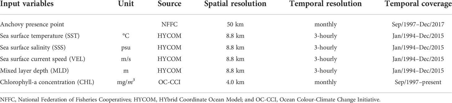
Table 1 The input dataset for the anchovy (Engraulis japonicus) MaxEnt construction.

The catch data used in this study contained no information on fishing gear, but according to the total anchovy catch production in Korea in 2006–2015 provided by the Statistics Korea, the anchovy was mainly caught using dragnets (56%), set nets (6.8%), and stow nets (5.7%). The dragnets and set nets primarily target juveniles (Kim and Lo, 2001). In Korea, the dragnets are prohibited from April to June in the northern ECS to protect the anchovy spawning biomass and early life stages, and also in the ES as the gears have possibly caused damage to other fishing equipment, including gill nets and fish pots. Therefore, the number of the presence points is relatively small in spring and in the ES (Figure 2B).

The anchovy presence data with a 0.5° spatial resolution were subdivided into four sub-grids of 0.25° as a larger dataset allowed for a greater range of MaxEnt features (Merow et al., 2013). For instance, if there were eight presence points in a 0.5° grid (i.e., the anchovy appeared eight times) during the study period, it is considered that a subdivided grid with 0.25° also has eight presence points. This subdivision method was acceptable since the environmental data had higher resolutions than the presence data. The four sub-grids were from one large grid, but since the environment data were at a high resolution, each sub-grid corresponded to different values for the environmental data. Consequently, a total of 257 grids in winter, 164 grids in spring, 361 grids in summer, and 487 grids in fall were used to project the seasonal habitat distribution of the anchovy in Korean waters (Figure 2). Data from the anchovy presence points showed high seasonal variability: in winter and spring, the presence points were mainly distributed on the northeastern part of the ECS, but in summer and fall, the points had a wider spread, mainly along the ES and the YS coasts in Korean waters (Figure 2).

Input data: Environmental data

A total of five environmental variables were available for the MaxEnt that were likely to affect the anchovy distribution: SST, sea surface salinity (SSS), sea surface current speed (VEL), MLD, and CHL (Table 1). These environmental predictors from 2000–2015 for the MaxEnt were sourced from HYbrid Coordinate Ocean Model GOFS 3.1 reanalysis data (Cummings, 2005) for SST, SSS, VEL, and MLD, and the Ocean Colour-Climate Change Initiative (Sathyendranath et al., 2020) for CHL (Table 1). The MLD was defined by a threshold method (Δ T=0.2°C) with a finite-difference criterion from a near-surface reference using water densities from temperature and salinity profiles (de Boyer Montégut et al., 2004). These high-resolution data had a horizontal resolution of 0.088° and 0.04° and were interpolated into a 0.25° grid, corresponding to the grid of the anchovy presence data.

The anchovy is distributed between the surface and mid-water or near the bottom layer (approximately 50–70 m) in Korean waters (Kang et al., 2014). The surface environmental variables were used in this study. Given that there were strong correlations between 0, 10, 30, and 50 m for both temperature and salinity and that the available environmental information for the shallow region reduced with increasing depth, environmental variables at the surface layer were selected.

MaxEnt construction

To estimate the anchovy habitat distribution in Korean waters, including the ES, YS, and ECS (Figure 1), the MaxEnt version 3.4.1k (https://biodiversityinformatics.amnh.org/open_source/maxent/) was used. MaxEnt is a commonly used machine learning based SDM shown to outperform in previous studies (Elith et al., 2006; Giovanelli et al., 2010), and the model is widely used in marine realms (Mugo et al., 2014; Alabia et al., 2016; Wang et al., 2018) as well as terrestrial, freshwater realms. MaxEnt requires presence-only data and environment covariates to estimate the presence probabilities, and in this study, the outputs were called the logistic habitat suitability index (HSI), with values ranging from 0 (lowest probability) to 1 (highest probability). MaxEnt uses the environmental covariates at species presence and background points (which can be replaced with pseudo-absences; Elith et al., 2006) to find the probability distribution of maximum entropy (i.e., most spread out or closest to uniform) and then constraint the distribution using environmental covariates at species presence. The HSI can provide explicit descriptions of how a habitat is defined, but it is unclear whether the HSI is a representative measure of relative abundance (Gomes et al., 2018).

FIGURE 1

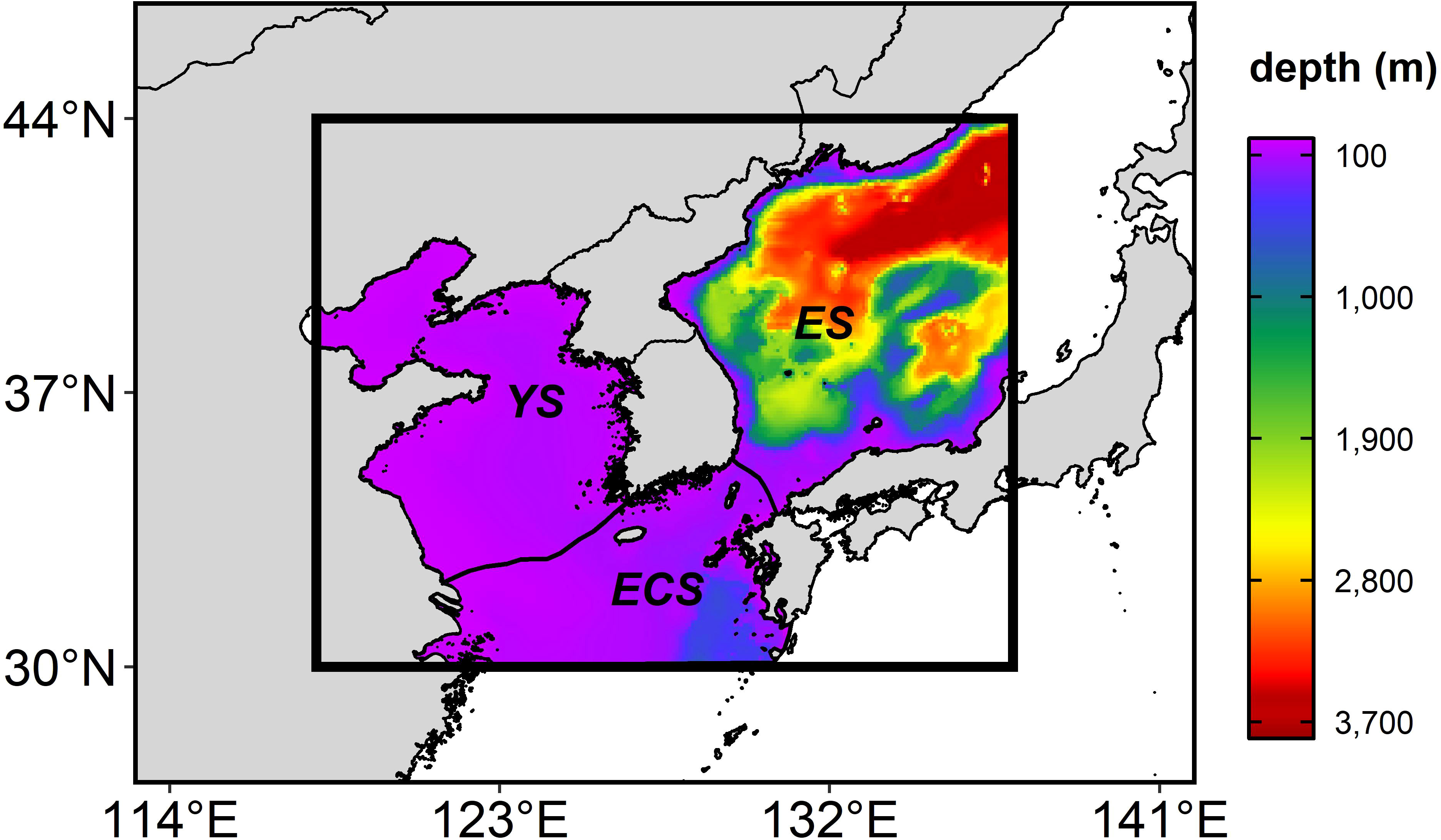
Figure 1 The study area (the thick box) (118-137°E and 33-44°N), including the East Sea (ES), the Yellow Sea (YS), and the East China Sea (ECS), overlaid with bathymetry (shade). The regional ocean boundaries are defined by the Large Marine Ecosystems Hub (https://www.lmehub.net/).

The anchovy presence points were randomly partitioned into a training set (75%) and a test set (25%), and the process was repeated ten times (10-fold cross-validation), with the average of the repetitions being presented as the results. The background points should be extracted to contrast against the presence locations (Merow et al., 2013). In this study, the background points were randomly selected from the environmental data within 300 km of the presence points, which could achieve approximately 10,000 background points—the default and recommended value for MaxEnt (Barbet-Massin et al., 2012). The number of background points per year was determined, with equal weight given to the presence points per year for model development. The final number of background points for the MaxEnt was 9,544 for winter, 10,003 for spring, 10,000 for summer, and 9,999 for fall.

MaxEnt has two main modifiable parameters: the feature class and the regularization multiplier (Morales et al., 2017). The six feature classes correspond to a mathematical transformation of the different covariates that are used in the model to allow for the complex relationships to be modeled, which include linear (L), product (P), quadratic (Q), hinge (H), threshold (T), and categorical (C; Elith et al., 2010). The feature is automatically selected using ‘auto-features’ and depends on the sample size of the training data (Morales‐Castilla et al., 2017). The regularization multiplier prevents over-complexity and overfitting, and the default value is 1 (Phillips and Dudík, 2008). Lower values of the regularization multiplier shift toward fitting the model closer to the presence points, and the higher values will progressively generalize the model and smooth out the response curves (O’Banion and Olsen, 2014). The default settings of ‘auto-feature’ and a regularization multiplier of 1 are not always the most effective (Syfert et al., 2013). Therefore, to decide on the best model, six feature class combinations (L, LQ, H, LQH, LQHP, and LQHPT) and ten regularization multipliers (0.5, 1.0, 1.5, 2.0, 2.5, 3.0, 3.5, 4.0, 4.5, and 5.0) were used. These were suggested as case studies in the ENMeval package (Muscarella et al., 2014).

The model performances were evaluated using the area under the curve (AUC) of the receiver operating characteristic (ROC) curve, widely used to evaluate the predictive performance of SDMs. A ROC curve is created by the true positive rate—the proportion of instances correctly predicted as presence—on the y-axis, against the false positive rate—the proportion of instances of absence wrongly predicted as presence—on the x-axis, and the area underneath the ROC curves, as an AUC, provided a measure of model performance in the SDM, where it can be classified as failing (0.5–0.6), bad (0.6–0.7), reasonable (0.7–0.8), good (0.8–0.9), or great (0.9–1) (Swets, 1988). In this study, The MaxEnt was evaluated by the mean values of ten replicates for the training and testing AUC values, and the models with the highest testing AUC values were selected as the best models from the 60 combination models (six feature classes and ten regularization multipliers).

Moreover, the continuous outputs of the MaxEnt were converted into binary maps as habitat versus non-habitat using the 10^th percentile training presence. The threshold was calculated as the 10^th percentile of the HSI at the training presence points, and the areas with an HSI higher than the threshold were distinguishable the anchovy habitat. This threshold is commonly used in MaxEnt studies (Kershaw et al., 2013; Padalia et al., 2014).

Future projection of the anchovy habitat distribution

Future changes in the anchovy HSI in Korean waters during the 2050s (2050–2059) were projected using the Coupled Model Intercomparison Project Phase 5 (CMIP5) global circulation models (GCMs) from the Intergovernmental Panel on Climate Change (IPCC) under the three Representative Concentration Pathway (RCP) climate change scenarios: RCP 2.6, RCP 4.5, and RCP 8.5. The three pathways represent mitigation, stabilization, and business-as-usual scenarios assuming low, medium, or high greenhouse gas emissions, respectively, by 2100. Seven GCMs provided the source environment variables from the historical data, and the three RCPs were selected: CanESM2, CNRM-CM5, HadGEM2-ES, IPSL-CM5A-LR, IPSL-CM5A-MR, MPI-ESM-LR, MPI-ESM-MR (Table 2). The future changes in the HSI were presented with a multi-model ensemble. The coarse resolution of the seven GCMs was interpolated into a finer grid at 0.25° to correspond with the subdivided anchovy presence data using bilinear interpolation. To reduce the bias of the GCMs, a delta method, a widely used bias-correction technique, was applied. The delta method is designed to use differences (Δ ) between the present and future data derived from the GCMs to correct for bias, and this was added to the present reanalysis or observation dataset (Navarro-Racines et al., 2020). To apply this method, the reference period of the variables from the HYbrid Coordinate Ocean Model, including the SST, SSS, VEL, and MLD, was set to 1994–2005, and the CHL from the Ocean Colour-Climate Change Initiative was set to 1998–2005. The reference period was the common period for the GCMs’ historical data and each set of observation/reanalysis data. The delta method was applied as follows:

$$\Delta T=T_{GCM}\left(future\right)- T_{GCM}\left(historical\right)$$

$$T^\left(future\right)=\Delta T+ T_{reanalysis}\left(historical\right)$$

TABLE 2

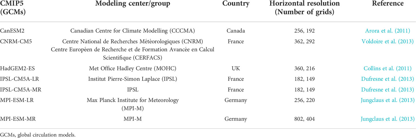
Table 2 List of the Coupled Model Intercomparison Project Phase 5 (CMIP5) models for the projection of the anchovy (Engraulis japonicus) habitat in Korean waters.

where $T^\left(future\right)$ indicates the bias-corrected GCMs output in the future. T_GCM(historical) and T_GCM(future) represent the output of the GCMs in the historical reference period and the future, respectively. T_reanalysis(historical) represents the reanalysis/observation data in the historical reference period.

The anchovy habitat gain and loss were calculated by dividing differences in the habitat area between future and historical periods by the total area of each region. The coverage of the future anchovy habitat was calculated by dividing the future habitat area by the total area of each region.

Results

Habitat model evaluation

The mean training and testing AUC in all the seasons were above 0.85, indicating that the seasonal MaxEnt has a high level of accuracy in model predictions (Table 3): the mean training and mean testing AUC values were 0.92, 0.91, 0.88, and 0.85 and 0.93, 0.94, 0.88, and 0.85 in winter, spring, summer, and fall, respectively. Small differences between the training and testing AUC values were in the range of -0.03–0.01, indicating low overfitting in the models (Warren and Seifert, 2011; Table 3).

TABLE 3

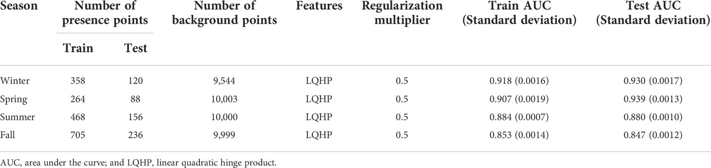
Table 3 Description and performance measures of the best MaxEnt.

Habitat characteristics of the anchovy derived from the MaxEnt

Of the five environmental variables used for the MaxEnt construction, SST, SSS, and CHL were the primary factors determining the historical habitat of the anchovy; however, the primary contribution depended on the season (Figure 3). In winter, the SST contributed the most (46.2%), followed by SSS (24.2%), VEL (14.0%), CHL (8.3%), and MLD (7.3%). In spring, the SST contributed the most (49.5%), followed by SSS (28.0%), MLD (11.0%), VEL (7.3%), and CHL (4.3%). In summer, the SSS contributed the most (53.0%), followed by SST (23.9%), VEL (15.5%), CHL (4.8%), and MLD (2.9%). In fall, the CHL contributed the most (48.4%), followed by MLD (17.4%), SST (12.5%), VEL (11.7%), and SSS (10.0%).

FIGURE 2

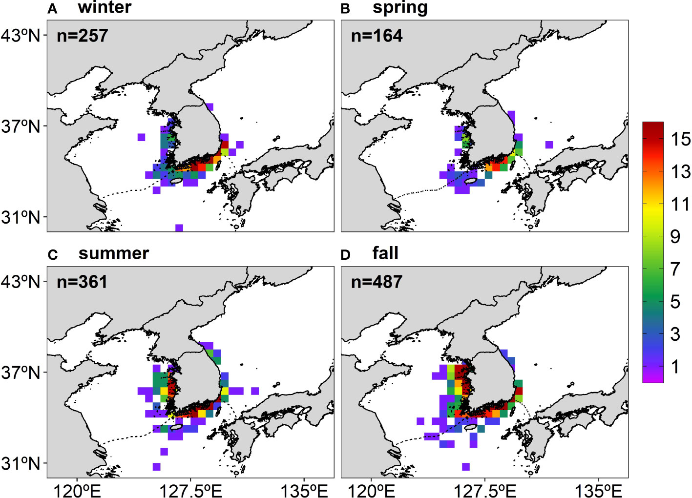
Figure 2 The number of the anchovy presence points for each season during the study period (16 years, 2000–2015) from the catch data archived by the National Federation of Fisheries Cooperatives in Korea: (A) winter, (B) spring, (C) summer, and (D) fall. The total number of presence points used for the MaxEnt construction is marked on the upper left side of each figure.

The map of the historical HSI for the anchovy was derived from the average yearly hindcasting from 2000–2015 (Figure 4). In winter and spring, the most suitable area was located mainly in the ECS (Figures 4A, B), and in summer and fall, it expanded northward along the Korean coast, reaching up to around 37°N in summer and over 38°N in fall (Figures 4C, D).

FIGURE 3

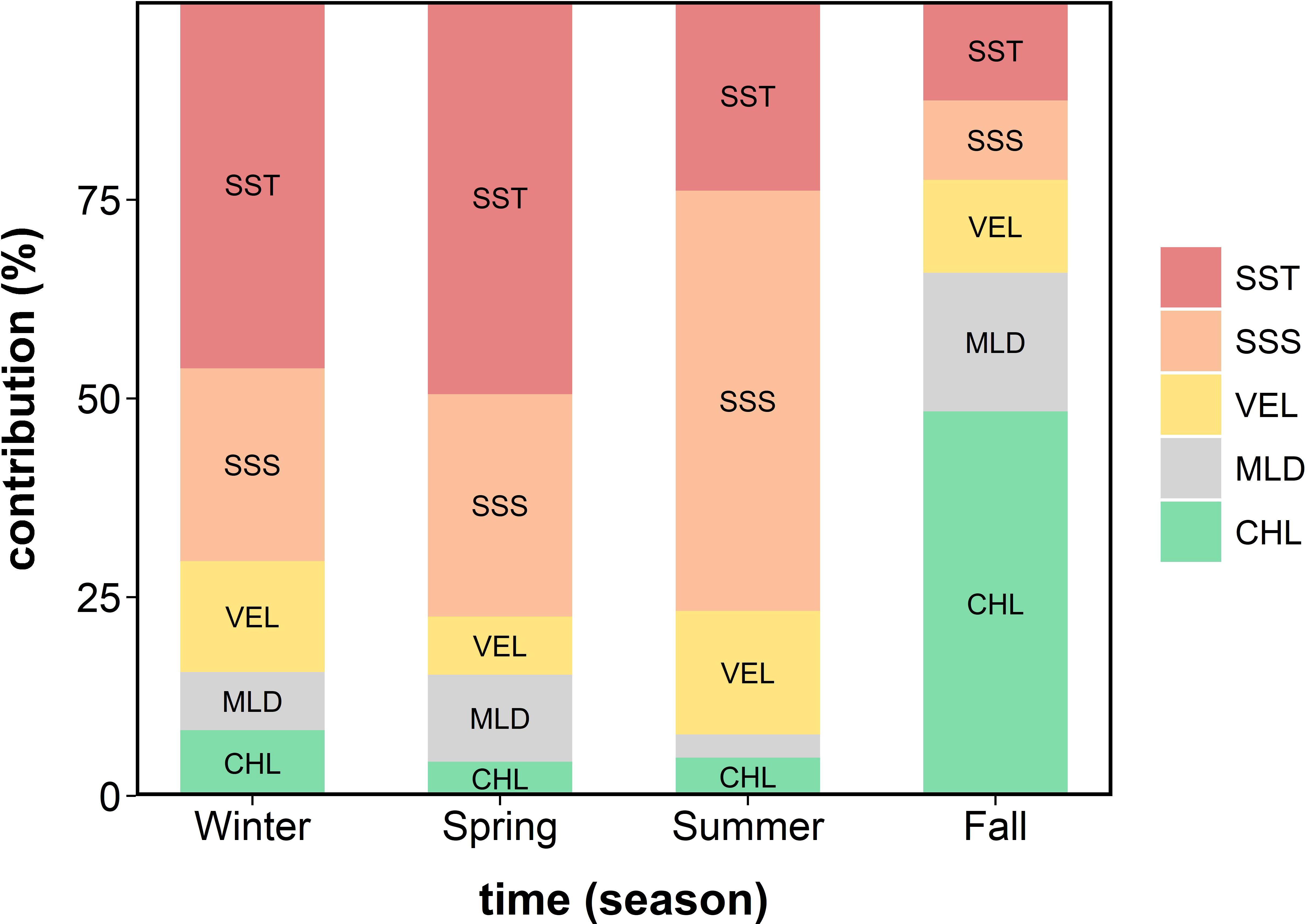
Figure 3 The seasonal variation in the relative contribution (%) of the five environmental variables for the potential anchovy habitat in Korean waters over 16 years (2000–2015) derived from the MaxEnt. SST, sea surface temperature; SSS, sea surface salinity; VEL, sea surface current speed; MLD, mixed layer depth; and CHL, chlorophyll-a concentration.

Future changes in the anchovy habitat distribution in Korean waters

In winter and spring, the HSI was projected to increase substantially in the southern ES and the southern YS and decrease in the ECS (Supplementary Figure 1). Meanwhile, in summer and fall, the HSI was projected to increase in the ES along the Korean coast and decrease in the YS and ECS (Supplementary Figure 1). These HSI changes are more pronounced for pathways with high carbon emissions, indicating rapid warming. As a result of the changes in the HSI distribution, the spatial distribution of the anchovy habitat also changed. The anchovy habitat is represented as a binary map showing areas where the anchovy habitat was in the historical period and where it will be in the future (Figure 5). The HSI thresholds were calculated to be 0.18 in winter, 0.15 in spring, 0.18 in summer, and 0.23 in fall, with the anchovy habitat being defined by the area with an HSI higher than the thresholds. In winter and spring, the habitat was projected to expand substantially northward to higher latitudes in the ES. However, in the ECS, a northward contraction in winter and a latitudinal expansion in spring were projected to occur in the future (Figures 5A, B). In summer and fall, the anchovy habitat was projected to expand northward along the coastal regions of North Korea in the ES, while contract northward in the ECS and coastward in the YS. In particular, a substantial contraction of the anchovy habitat was projected in the YS in the summer, and the habitat is no longer available under RCP 8.5 (Figures 5C, D).

FIGURE 4

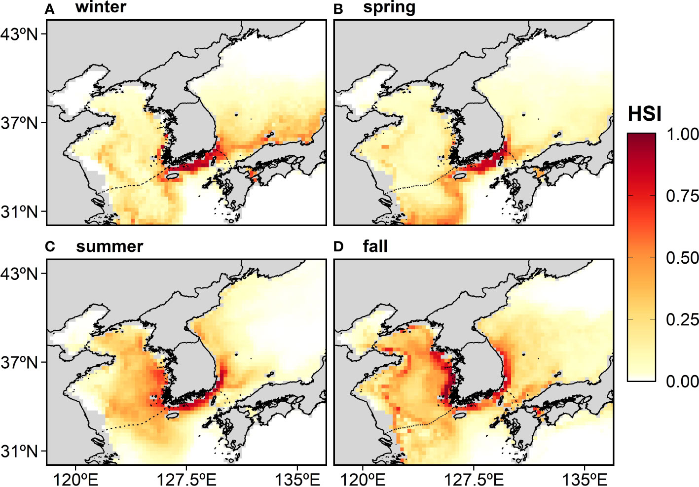
Figure 4 The distribution of the anchovy habitat suitability index (HSI) in Korean waters averaged over 16 years (2000–2015) and derived from the MaxEnt: (A) winter, (B) spring, (C) summer, and (D) fall. The reddish color indicates a highly suitable area or a high probability of occurrence.

The relative geographical areas provide information on the habitat gain or loss for the anchovy in Korean waters (Figure 6). The future changes in the anchovy habitat were projected to increase by 19.4–21.3% in winter and 32.1–38.4% in spring, while decreased by 13.1–19.4% in summer and 1.5–8.3% in fall within Korean waters under the three RCPs (Figure 6A). Substantial differences in the anchovy habitat area between the regional seas were identified. In the ES, the future habitat area was projected to increase in all the seasons under the three RCPs, with a considerable increase (39.4–48.3%) observed during spring (Figure 6B). In contrast, in the YS and the ECS, the future habitat area was projected to increase in winter and spring and decrease in summer and fall (Figures 6C, D). In winter and spring, the YS and the ECS showed positive habitat changes, increasing by 19.9–42.8% in the YS and 2.0–17.4% in the ECS. In contrast, in summer and fall, the YS and the ECS showed negative changes, decreasing by 12.2–60.8% in the YS and 12.2–23.9% in the ECS (Figures 6C, D).

FIGURE 5

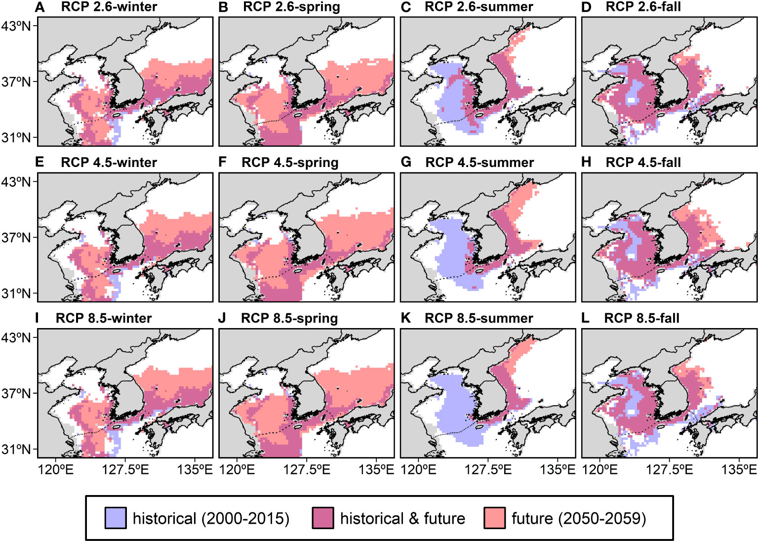
Figure 5 The seasonal changes in the spatial distribution of the anchovy habitat in the past (2000–2015) and future (the 2050s) under RCP 2.6 (A–D), RCP 4.5 (E–H), and RCP 8.5 (I–L) represent low (mitigation), medium (stabilization), or high (business-as-usual) greenhouse gas emissions, respectively. The anchovy habitat defined areas with HSIs above the 10^th percentile of the training presence as thresholds. Blue indicates historical habitat, pink indicates future habitat, and purple indicates the habitat in both the historical period and the future. RCP; representative concentration pathway.

Major drivers of the future changes in the anchovy habitat distribution in Korean waters

To identify the main drivers of the climate-induced changes in the anchovy habitat distribution in Korean waters, the relationships between the HSI and the top three environmental factors (SST, SSS, and CHL) selected by their contribution, as derived from MaxEnt (Figure 3) and the environmental variables at the anchovy presence points in both the historical and future period, are presented (Figure 7). Non-linear relationships existed between the environment variables as the predictor and the HSI as the response variable. The response of the SST was unimodal from winter to summer: the highest habitat probabilities were 16.6°C in winter, 14.9°C in spring, and 21.0°C in summer (Figures 7A–C). However, a bimodal response of the SST occurred in the fall, with peak probabilities at 19.2°C and 22.9°C (Figure 7D). The response of the SSS was also unimodal, with the highest probabilities at 32.7 psu in winter, 32.2 psu in spring, 33.0 psu in summer, and 32.4 psu in fall (Figures 7E–H). The CHL response curves showed a peak of 0–1 mg/m³ in all the seasons (Figures 7I–L). The small standard deviations in the response curves for the SST, SSS, and CHL of the ten replicated MaxEnt runs for all the seasons indicate that the HSI can be consistently predicted and that the constructed models are robust. The main contributors depended on the seasons according to the MaxEnt output when using historical data.

FIGURE 6

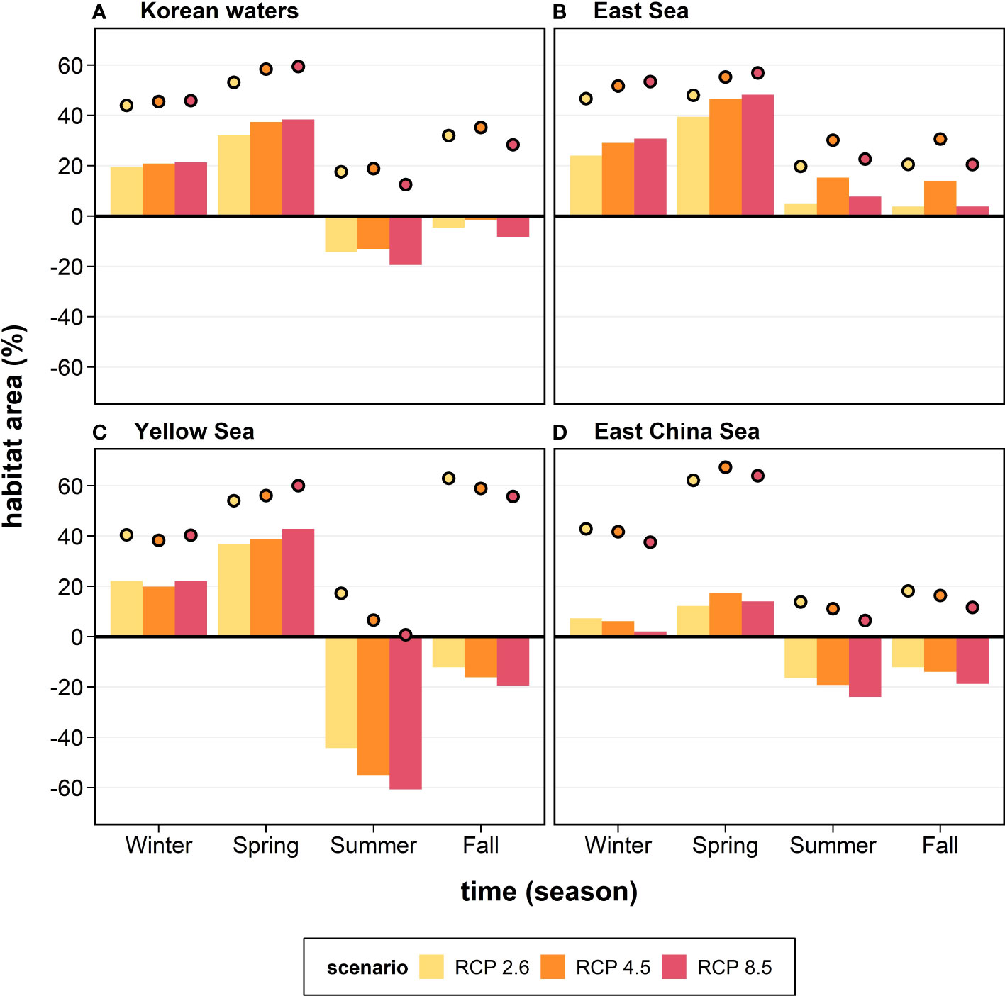
Figure 6 The anchovy habitat gain and loss (%; bars) in the future (the 2050s) under the three different future scenarios (colors) in each region: (A) Korean waters, (B) the East Sea, (C) the Yellow Sea, and (D) the East China Sea. The habitat gain and loss are the differences in the habitat area between future (the 2050s) and historical (2000–2015) periods divided by the total area of each region. The coverage (closed circles) of the future anchovy habitat (%) relative to the total area of each region is also shown.

However, the environmental contributors of the anchovy distribution estimated from the historical data and the major drivers of the future changes may differ. The CMIP5 multi-model ensemble used in the current study projected that Korean waters would undergo an SST increase (1–3°C), SSS decrease (maximum 0.5 psu), and CHL decrease (maximum 2 mg/m³) in all the seasons under the three RCPs in the 2050s. Thus, for the historical presence points of the anchovy, the environmental variables are projected to change in the future. Under RCP 8.5, as SST increases due to global warming, the SST ranges at the anchovy presence points were projected to include SSTs with a high HSI in winter and spring, while the ranges appear to deviate from the SSTs with a high HSI in summer and fall (Figures 7A–D). As SSS decreases in the future, the SSS ranges at the presence points were projected to include the SSSs with a high HSI in winter and spring, while the ranges tend to deviate and contract from the SSSs with a high HSI in summer and fall, respectively (Figures 7E–H). In the case of CHL, substantial changes were observed between the past and the future, mainly due to changes in the maximum values of the ranges from 5.0 mg/m³ to 9.3 mg/m³ in all the seasons (Figures 7I–L). Therefore, in winter and spring, the SST and SSS ranges cover the thermal and saline optima, but in summer and fall, there is a deviation from the optima. Among the two variables, given that the SST changes are greater than salinity, the HSI changes are likely related to the SST. This suggests that the anchovy habitat in Korean waters is likely to change with SST changes in the future.

Discussion

Spatial and temporal distributions of the anchovy

The spatial distribution of the HSI according to the historical (2000–2015) data based on MaxEnt reflects the distribution of the presence points for the anchovy over the same period (Figure 2) and previous studies (Kim et al., 2020). For all the seasons, the highest predicted HSI for the anchovy occurred in the ECS—one of the main spawning grounds for the anchovy in Korean waters (Figure 4). In the ECS, the anchovy catch productivity was more than 200,000 t, accounting for 88% of the total anchovy catch in Korean waters in 2000–2015 from the Statistics Korea database. The total anchovy catch was also high in the areas with a high HSI. In the YS and the ES, the HSI was high in summer and fall, consistent with the anchovy migration route in Korean waters. The anchovy moves from the ECS to the central ES and the northern YS with the East Korea Warm Current that branches off the Tsushima Warm Current in the ES and the Yellow Sea Warm Current that branches off the Kuroshio Current in the YS and expands northward during late spring and early summer (NFRDI, 2010).

FIGURE 7

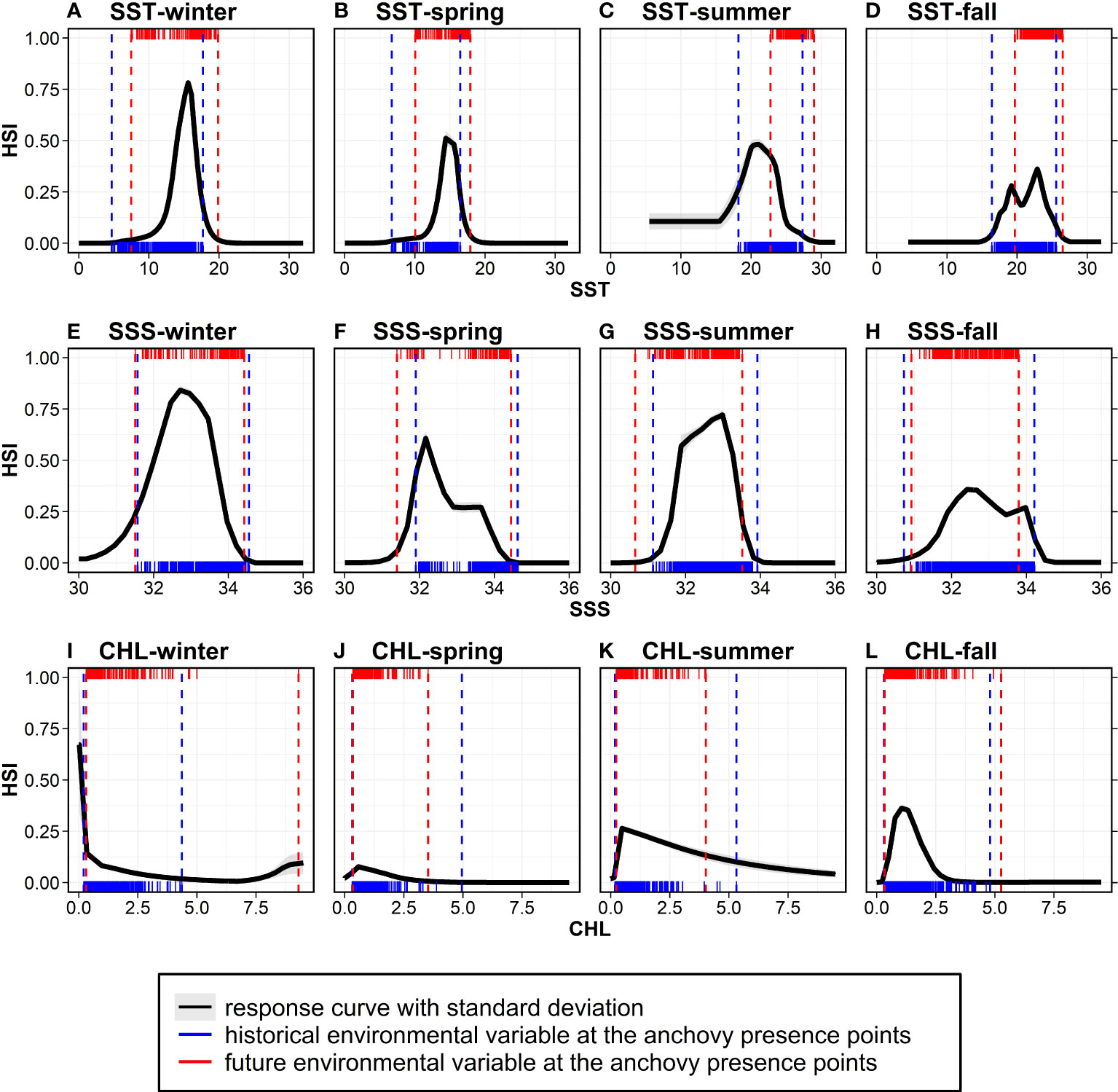
Figure 7 The species response curves of the environmental variables derived from the MaxEnt: (A–D) SST, (E–H) SSS, and (I–L) CHL from winter to fall. Black solid lines and grey shading indicate the averages and standard deviations of the ten replicated responses. Blue rug plots indicate the values of the environmental variables at the anchovy presence points, and blue vertical dashed lines show the ranges of the environmental variables (minima and maxima of the blue rug) during the study period (2000–2015). The red rug plots indicate the future environmental variables at the anchovy presence points (identical points to the historical period), and the red vertical dashed lines show the future environmental ranges under RCP 8.5. HSI, habitat suitability index.

The contributions of environmental variables in the MaxEnt indicate that CHL was one of the strongest determinants in the anchovy habitat in the fall (Figure 3). The CHL is related to anchovy feeding habitat, and the seasonal variations in CHL are highly affected by phytoplankton bloom which occurs in spring and fall (Yamada et al., 2004; Kim et al., 2006; Oh and Suh, 2006). Although phytoplankton bloom is more considerable in spring than in fall, the CHL contribution was not high in spring. This might be because CHL could not be limiting factor for the anchovy distribution since high CHL was distributed widely in spring. The optimum CHL—areas with CHL higher than the 10^th percentile of the temporally averaged CHL during 2000–2015 at the anchovy presence points—prevailed in Korean waters in the spring and the YS in the fall (Supplementary Figure 2). In contrast, the distribution was limited to the ECS and the ES in the fall (Supplementary Figure 2B). Therefore, the substantial contribution of CHL to anchovy distribution in the fall seems to be associated with CHL acting as a limiting factor for anchovy distribution.

Projected future changes in the anchovy habitat area in Korean waters under the three RCPs from the lowest to highest CO₂ emissions (RCP 2.6, RCP 4.5, and RCP 8.5) using the CMIP5 showed considerable seasonal variation. Global warming was found to provide favorable habitat for the anchovy in the ES throughout the year and the YS and the ECS in winter and spring, while unfavorable habitat in the YS and the ECS in summer and fall. Based on predicted model outputs for the 2030s under the Special Report on Emission Scenarios A1B, which indicates emission scenarios with medium CO₂ concentrations (703 ppm in 2100) from the CMIP3, during summer, the larval anchovy biomass was projected to decrease in the YS and the ECS but increase in the ES (Jung et al., 2016). During fall, a decrease in the larval anchovy biomass was predicted, except for the southeastern part of the ES in the 2030s (Jung et al., 2016). Furthermore, it is expected that wintering anchovy will be positively affected by global warming based on the positive correlations between the anchovy CPUE in winter and temperature using historical data (Niu et al., 2014; Niu and Wang, 2017; Liu et al., 2020). These seasonal and regional changes in the biomass of the anchovy in early life stages based on previous research (Niu et al., 2014; Jung et al., 2016; Niu and Wang, 2017; Liu et al., 2020) were largely consistent with the spatial-temporal changes in the projected HSI in the future with climate change in this study.

The individual size of the anchovy caught in Korean waters mainly depends on the fishing season, and small-sized anchovy, in the juvenile stage, accounts for a significant portion of the anchovy catch in Korean waters (NFRDI, 2010). The immatures are generally considered more vulnerable to environmental changes in the early life stages compared to adults (Halley et al., 2018) due to a narrow tolerance range (Dahlke et al., 2020). Thus, the HSI changes are likely to affect the population size through recruitment and survival in their early life stages.

Future changes in the spawning habitat suitability of the anchovy

Based on the results of this study, during the summer, the peak spawning season of the anchovy, the HSI was projected to substantially decrease in the ECS and the YS, which are major anchovy spawning grounds. The spawning ground, where marine organisms mate, spawn, hatch, and breed, is critical for small pelagic fish, primarily in the larval stages when they are most vulnerable to environmental change. In the western North Pacific, egg production (Kim and Lo, 2001; Takasuka et al., 2005), the mortality rate at the embryonic stage (Kim and Lo, 2001), and recruitment (Yu et al., 2020) are affected by environmental factors, such as temperature, salinity, and food availability. In the North Sea, an increase in the abundance of European anchovy (E. encrasicolus) originated from improved the population productivity associated with an expansion in the thermal habitat (Petitgas et al., 2012). In southern Benguela, a decline in the population biomass of anchovy (E. capensis) was affected by declining egg abundance resulting from a decrease in the spawning area during 1984–1998 (Van der Lingen et al., 2001). Based on the findings of previous studies, habitats in the early life stages determines population size and can decrease recruitment through the mortality of the fish species.

The future changes in the anchovy HSI were projected to increase in the ES in all the seasons. The anchovy adults migrate inshore for spawning (Choi et al., 2001; Kim and Lo, 2001), with the eggs and larvae located in the coastal area (Kang et al., 1996; Shin et al., 2021). They inhabit shallow water ranging from 0–100 m (Kang et al., 1996) and mainly inhabit the surface layer in the early life stages (Iseki and Kiyomoto, 1997). Unlike the YS and the ECS, which are characterized by a shallow depth of less than 100 m and complex coastlines due to the archipelago structure, the ES has a less topographically complex coastline, with an average depth of 1,700 m (Figure 1). If the ES replaces the current spawning grounds for the anchovy, successful transport to the coastal area may be an important contributing factor to the habitat of the early life anchovy. Therefore, continuous monitoring is necessary to evaluate whether the ES can serve as the new spawning ground of the anchovy. If the ES is to be a newly spawning ground of the anchovy, it is necessary to effectively respond to climate change by expanding the current closure area in the ECS to ES.

Fish can avoid unfavorable spawning habitats by relocating the spawning area and changing the timing of reproduction. A few studies have documented phenological changes in spawning periods due to environmental changes. In the northeast Pacific, a prolonged spawning duration due to anomalous warm conditions was observed for northern anchovy (E. mordax) in 2015–2016 using ichthyoplankton sampling (Auth et al., 2018). In the Bay of Biscay, an advanced peak spawning for European anchovy was observed at a rate of 5.5 days/decade from 1987–2015, with an increasing gonadosomatic index, which might be associated with changes in phytoplankton abundance (Erauskin-Extramiana et al., 2019). The anchovy target species in this study also showed an increase in the total reproductive effort due to the shortening of batch intervals in water at a higher temperature based on a rearing experiment (Yoneda et al., 2014). With the changes in the distribution of anchovy spawning grounds, the spawning date might change as well, and thus, the currently enforced fishing closure from April to June in Korean waters for the protection of the anchovy spawning biomass may need to be adjusted in the future depending on the impact of climate change. There are possibilities of temporal mismatches between fish in early life stages and prey due to the changes in the spawning date, which may also negatively affect the anchovy abundance.

Limitations and future studies

The anchovy mainly feed on zooplankton and phytoplankton (Kim et al., 2013; Kim et al., 2017), but zooplankton was not considered directly in this study since the zooplankton biomass data from the Korea Ocean Data Center have a narrower spatial distribution than the area required for MaxEnt construction. Thus, the CHL, as an indicator of phytoplankton, which is associated with changes in zooplankton biomass (Kang and Kim, 2008; Kim and Kang, 2020), was considered in this study.

In addition, there are limitations to the fisheries-dependent data we used since the data are affected by the issues faced by fisheries. The data have biases in (1) a catch (quantitative bias) of species, such as catchability depending on fishing gears, quality control, standardization in data collection, and misreporting catches (Olin and Malinen, 2003; Thorson and Simpfendofer, 2009; Pennino et al., 2016; Orue et al., 2020) and (2) spatial distribution. The catch bias would be negligible since only the presence data were used in this study. The primary issues are spatial biases from preferential sampling by fishing fleets driven commercially and constraints imposed by management (Pennino et al., 2016; Orue et al., 2020). For instance, the anchovy population is widely distributed in Korean waters based on our results (Figures 4, 5) and previous studies (Kim et al., 2020). However, the anchovy fisheries mainly operate in the coastal regions (Figure 2), probably due to the high catch density and efficiency at the shallow depths, and the economic cost of being close to the coast. Due to the bias in the the presence point distribution focusing on coastal areas, coastal environmental data would be considered more in the MaxEnt. With regard to constraints imposed by management, model uncertainties could arise from the prohibition of the anchovy dragnets, responsible for up to 50–60% of the total anchovy catch (Kim and Lo, 2001), in the spring and in the ES through insufficient reflections of the anchovy presence. Furthermore, it is possible that MaxEnt with the fisheries-dependent data would project a stricter distribution of the anchovy habitat than the fishery-independent data (DiNardo et al., 2021). Fisheries-independent data (scientific survey data) could reduce bias and uncertainty because sampling statistics and the biological information of the target species-area are considered during survey design (Pennino et al., 2016). Estimating the anchovy distribution using fisheries-independent datasets is also needed for future studies.

Implications

Despite these uncertainties, this study has provided a comprehensive understanding and identified threats to the anchovy habitat under climate change to ensure sustainable yields of the anchovy in the future. This study suggests some possibilities for the seasonal changes in the spatial distribution of the anchovy habitat in Korean waters, and the HSI changes are more pronounced for pathways with high carbon emissions, indicating rapid warming under climate change scenarios from the lowest to the highest CO₂ emissions using seven GCMs. Under RCP 2.6, the changes in the anchovy habitat distribution are relatively minor, while under RCP 8.5, substantial habitat losses were projected in Korean waters, with a complete disappearance in the YS during the major spawning period. If the rate of climate change is controlled, the rate of changes in the anchovy distribution resulting from global warming may be reduced. These results hold value in guiding the maintenance of the potential productivity of ocean and ecosystem services. Therefore, the effects of climate change on the seasonal distribution of fisheries resources should be considered in the planning of future management strategies, including the development of fisheries-independent monitoring in Korean waters in the context of climate change, particularly for environmentally sensitive species.

Conclusion

This study investigated potential future changes in the seasonal distribution of the anchovy (Engraulis japonicus) habitat in Korean waters using a maximum entropy model with anchovy presence points and five environmental variables. It was found that the anchovy habitat in the 2050s can undergo seasonal variations, with a northward expansion in winter and spring and a coastward reduction in the Yellow Sea during summer and fall. The sea surface temperatures in winter and spring were close to the lower boundaries of the thermal optimum for the anchovy in Korean waters, while the sea surface temperatures in summer and fall were close to the higher boundary of the thermal optimum for the anchovy. An increase in water temperature due to global warming could contribute to habitat gain in winter and spring and habitat loss in summer and fall. In summer, the summer could experience substantial habitat loss in the Yellow Sea and the East China Sea, which are the main spawning grounds in Korean waters, and this might lead to a biomass reduction, relocation of spawning areas, and changes in the timing of reproduction. Findings from the current study suggest that seasonal differences in future fish distributions should be considered for planning future management strategies, including evaluation of spawning grounds projected to be newly replaced, adjustment of the fishing closure period from potential changes in the spawning date, limiting the current closure period in only the East Sea, projected replaced spawning habitat.

Data availability statement

The original contributions presented in the study are included in the article/Supplementary Material. Further inquiries can be directed to the corresponding author.

Author contributions

MB and CJ devised the main conceptual ideas and carried out the experiments. DS encouraged MB to set the model configuration. JK and CK collected the fisheries data and interpreted the results. WC collected oceanographic data and calculated the oceanic variables. All authors contributed to defining the scope of the research, provided critical feedback, and assisted in shaping the discussion of the research.

Funding

This work was funded by the National Institute of Fisheries Science as part of the project "An investigation on the rigorous analysis for fluctuation of fishing condition and the advancement for fishing forecasting in the Korean waters (R2022040)" and the Korea Meteorological Administration, as a part of the projects "Projection and evaluation of ocean climate and extreme events based on AR6 scenarios (KMI2021-01511)".

Acknowledgments

First of all, we would like to thank Dr. Sukyung Kang for giving us the opportunity to start this research project and for her valuable and constructive suggestions during the planning and development of this research work. We also acknowledge the World Climate Research Programme’s Working Group on Coupled Modelling, which is responsible for CMIP, and we thank the climate modeling groups (listed in Table 2 of this paper) for producing and making available their model output. For CMIP, the U.S. Department of Energy’s Program for Climate Model Diagnosis and Intercomparison provides coordinating support and leads the development of software infrastructure in partnership with the Global Organization for Earth System Science Portals.

Conflict of interest

The authors declare that the research was conducted in the absence of any commercial or financial relationships that could be construed as a potential conflict of interest.

Publisher’s note

All claims expressed in this article are solely those of the authors and do not necessarily represent those of their affiliated organizations, or those of the publisher, the editors and the reviewers. Any product that may be evaluated in this article, or claim that may be made by its manufacturer, is not guaranteed or endorsed by the publisher.

Supplementary material

The Supplementary Material for this article can be found online at: https://www.frontiersin.org/articles/10.3389/fmars.2022.922020/full#supplementary-material

References

Alabia I. D., Saitoh S. I., Igarashi H., Ishikawa Y., Usui N., Kamachi M., et al. (2016). Ensemble squid habitat model using three-dimensional ocean data. ICES. J. Mar. Sci. 73 (7), 1863–1874. doi: 10.1093/icesjms/fsw075

CrossRef Full Text | Google Scholar

Alheit J., Licandro P., Coombs S., Garcia A., Giráldez A., Santamaría M. T. G., et al. (2014). Reprint of “Atlantic multidecadal oscillation (AMO) modulates dynamics of small pelagic fishes and ecosystem regime shifts in the eastern north and central atlantic”. J. Mar. Syst. 133, 88–102. doi: 10.1016/j.jmarsys.2014.02.005

CrossRef Full Text | Google Scholar

Arora V. K., Scinocca J. F., Boer G. J., Christian J. R., Denman K. L., Flato G. M., et al. (2011). Carbon emission limits required to satisfy future representative concentration pathways of greenhouse gases. Geophys. Res. Lett. 38 (5), L05805. doi: 10.1029/2010GL046270

CrossRef Full Text | Google Scholar

Auth T. D., Daly E. A., Brodeur R. D., Fisher J. L. (2018). Phenological and distributional shifts in ichthyoplankton associated with recent warming in the northeast pacific ocean. Glob. Change Biol. 24 (1), 259–272. doi: 10.1111/gcb.13872

CrossRef Full Text | Google Scholar

Barange M., Merino G., Blanchard J. L., Scholtens J., Harle J., Allison E. H., et al. (2014). Impacts of climate change on marine ecosystem production in societies dependent on fisheries. Nat. Clim. Change 4 (3), 211–216. doi: 10.1038/nclimate2119

CrossRef Full Text | Google Scholar

Barbet-Massin M., Jiguet F., Albert C. H., Thuiller W. (2012). Selecting pseudo-absences for species distribution models: how, where and how many? Methods Ecol. Evol. 3 (2), 327–338. doi: 10.1111/j.2041-210X.2011.00172.x

CrossRef Full Text | Google Scholar

Belkin I. M. (2009). Rapid warming of Large marine ecosystems. Prog. Oceanogr. 81 (1-4), 207–213. doi: 10.1016/j.pocean.2009.04.011

CrossRef Full Text | Google Scholar

Cheung W. W., Lam V. W., Sarmiento J. L., Kearney K., Watson R. E. G., Zeller D., et al. (2010). Large-Scale redistribution of maximum fisheries catch potential in the global ocean under climate change. Glob. Change Biol. 16 (1), 24–35. doi: 10.1111/j.1365-2486.2009.01995.x

CrossRef Full Text | Google Scholar

Choi S. G., Kim J. Y., Kim S. S., Choi Y. M., Choi K. H. (2001). Biomass estimation of anchovy (Engraulis japonicus) by acoustic and trawl surveys during spring season in the southern Korean waters. J. Korean. Soc. Fish. Res. 4, 20–29.

Google Scholar

Choo H. S., Kim D. S. (1998). The effect of variations in the tsushima warm currents on the egg and larval transport of anchovy in the southern Sea of Korea. Korean. J. Fish. Aquat. Sci. 31 (2), 226–244.

Google Scholar

Ciannelli L., Bailey K. M. (2005). Landscape dynamics and resulting species interactions: the cod-capelin system in the southeastern Bering Sea. Mar. Ecol.-Prog. Ser. 291, 227–236. doi: 10.3354/meps291227

CrossRef Full Text | Google Scholar

Collins W. J., Bellouin N., Doutriaux-Boucher M., Gedney N., Halloran P., Hinton T., et al. (2011). Development and evaluation of an earth-system model–HadGEM2. Geosci. Model. Dev. 4 (4), 1051–1075. doi: 10.5194/gmd-4-543-2011

CrossRef Full Text | Google Scholar

Cummings J. A. (2005). Operational multivariate ocean data assimilation. Quart. J. R. Met. Soc. Part C. 131 (613), 3583–3604. doi: 10.1256/qj.05.105

CrossRef Full Text | Google Scholar

Cury P., Roy C. (1989). Optimal environmental window and pelagic fish recruitment success in upwelling areas. Can. J. Fish. Aquat. Sci. 46 (4), 670–680. doi: 10.1139/f89-086

CrossRef Full Text | Google Scholar

Dahlke F. T., Wohlrab S., Butzin M., Pörtner H. O. (2020). Thermal bottlenecks in the life cycle define climate vulnerability of fish. Science 369 (6499), 65–70. doi: 10.1126/science.aaz3658

PubMed Abstract | CrossRef Full Text | Google Scholar

de Boyer Montégut C., Madec G., Fischer A. S., Lazar A., Iudicone D. (2004). Mixed layer depth over the global ocean: An examination of profile data and a profile-based climatology. J. Geophys. Res.-Oceans. 109, (C12003). doi: 10.1029/2004JC002378

CrossRef Full Text | Google Scholar

DiNardo J., Stierhoff K. L., Semmens B. X. (2021). Modeling the past, present, and future distributions of endangered white abalone (Haliotis sorenseni) to inform recovery efforts in California. PloS One 16 (11), e0259716. doi: 10.1371/journal.pone.0259716

PubMed Abstract | CrossRef Full Text | Google Scholar

Drinkwater K. F. (2005). The response of Atlantic cod (Gadus morhua) to future climate change. ICES. J. Mar. Sci. 62 (7), 1327–1337. doi: 10.1016/j.icesjms.2005.05.015

CrossRef Full Text | Google Scholar

Dufresne J. L., Foujols M. A., Denvil S., Caubel A., Marti O., Aumont O., et al. (2013). Climate change projections using the IPSL-CM5 earth system model: from CMIP3 to CMIP5. Clim. Dyn. 40 (9), 2123–2165. doi: 10.1007/s00382-012-1636-1

CrossRef Full Text | Google Scholar

Dulvy N. K., Baum J. K., Clarke S., Compagno L. J., Cortés E., Domingo A., et al. (2008). You can swim but you can't hide: the global status and conservation of oceanic pelagic sharks and rays. Aquat. Conserv.-Mar. Freshw. Ecosyst. 18 (5), 459–482. doi: 10.1002/aqc.975

CrossRef Full Text | Google Scholar

Elith J., Graham C. H., Anderson R. P., Dudík M., Ferrier S., Guisan A., et al. (2006). Novel methods improve prediction of species’ distributions from occurrence data. Ecography 29 (2), 129–151. doi: 10.1111/j.2006.0906-7590.04596.x

CrossRef Full Text | Google Scholar

Elith J., Leathwick J. R. (2009). Species distribution models: ecological explanation and prediction across space and time. Annu. Rev. Ecol. Evol. Syst. 40, 677–697. doi: 10.1146/annurev.ecolsys.110308.120159

CrossRef Full Text | Google Scholar

Elith J., Phillips S. J., Hastie T., Dudík M., Chee Y. E., Yates C. J. (2010). A statistical explanation of MaxEnt for ecologists. Divers. Distrib. 17 (1), 43–57. doi: 10.1111/j.1472-4642.2010.00725.x

CrossRef Full Text | Google Scholar

Erauskin-Extramiana M., Alvarez P., Arrizabalaga H., Ibaibarriaga L., Uriarte A., Cotano U., et al. (2019). Historical trends and future distribution of anchovy spawning in the bay of Biscay. Deep-Sea. Res. Part II-Top. Stud. Oceanogr. 159, 169–182. doi: 10.1016/j.dsr2.2018.07.007

CrossRef Full Text | Google Scholar

Food and Agriculture Organization (2022) Aquatic species distribution map viewer. Available at: https://www.fao.org/figis/geoserver/factsheets/species.html (Accessed February 15, 2022).

Google Scholar

Franklin J. (2010). Mapping species distributions: Spatial inference and prediction (Cambridge: Cambridge University Press).

Google Scholar

Froose R., Pauly D. (2022) Fishbase. Available at: www.fishbase.org, version (Accessed February 15, 2022).

Google Scholar

Garrido S., Silva A., Marques V., Figueiredo I., Bryère P., Mangin A., et al. (2017). Temperature and food-mediated variability of European Atlantic sardine recruitment. Prog. Oceanogr. 159, 267–275. doi: 10.1016/j.pocean.2017.10.006

CrossRef Full Text | Google Scholar

Giovanelli J. G., de Siqueira M. F., Haddad C. F., Alexandrino J. (2010). Modeling a spatially restricted distribution in the neotropics: How the size of calibration area affects the performance of five presence-only methods. Ecol. Model. 221 (2), 215–224. doi: 10.1016/j.ecolmodel.2009.10.009

CrossRef Full Text | Google Scholar

Gomes V. H. F., Ijff S. D., Raes N., Amara I. L., Salomão R. P., de Souza Coelho L., et al. (2018). Species distribution modelling: Contrasting presence-only models with plot abundance data. Sci. Rep. 8 (1), 1–12. doi: 10.1038/s41598-017-18927-1

PubMed Abstract | CrossRef Full Text | Google Scholar

Halley J. M., Van Houtan K. S., Mantua N. (2018). How survival curves affect populations’ vulnerability to climate change. PloS One 13 (9), e0203124. doi: 10.1371/journal.pone.0203124

PubMed Abstract | CrossRef Full Text | Google Scholar

Hiddink J. G., Burrows M. T., García Molinos J. (2015). Temperature tracking by north Sea benthic invertebrates in response to climate change. Glob. Change Biol. 21 (1), 117–129. doi: 10.1111/gcb.12726

CrossRef Full Text | Google Scholar

Holsman K. K., Haynie A. C., Hollowed A. B., Reum J. C. P., Aydin K., Hermann A. J., et al. (2020). Ecosystem-based fisheries management forestalls climate-driven collapse. Nat. Commun. 11, 4579. doi: 10.1038/s41467-020-18300-3

PubMed Abstract | CrossRef Full Text | Google Scholar

Hwang S. D., McFarlane G. A., Choi O. I., Kim J. S., Hwang H. J. (2007). Spatiotemporal distribution of pacific anchovy (Engraulis japonicus) eggs in the West Sea of Korea. Fish. Aquat. Sci. 10 (2), 74–85. doi: 10.5657/fas.2007.10.2.074

CrossRef Full Text | Google Scholar

Iseki K., Kiyomoto Y. (1997). Distribution and settling of Japanese anchovy (Engraulis japonicus) eggs at the spawning ground off changjiang river in the East China Sea. Fish. Oceanogr. 6 (3), 205–210. doi: 10.1046/j.1365-2419.1997.00040.x

CrossRef Full Text | Google Scholar

Ito S. I., Okunishi T., Kishi M. J., Wang M. (2013). Modelling ecological responses of pacific saury (Cololabis saira) to future climate change and its uncertainty. ICES. J. Mar. Sci. 70 (5), 980–990. doi: 10.1093/icesjms/fst089

CrossRef Full Text | Google Scholar

Ji F., Guo X., Takayama K. (2020). Response of the Japanese flying squid (Todarodes pacificus) in the Japan Sea to future climate warming scenarios. Clim. Change 159, 601–618. doi: 10.1007/s10584-020-02689-3

CrossRef Full Text | Google Scholar

Jungclaus J. H., Fischer N., Haak H., Lohmann K., Marotzke J., Matei D., et al. (2013). Characteristics of the ocean simulations in the max planck institute ocean model (MPIOM) the ocean component of the MPI-earth system model. J. Adv. Model. Earth Syst. 5 (2), 422–446. doi: 10.1002/jame.20023

CrossRef Full Text | Google Scholar

Jung S., Pang I.-C., Lee J.-H., Choi I., Cha H. K. (2014). Latitudinal shifts in the distribution of exploited fishes in Korean waters during the last 30 years: a consequence of climate change. Rev. Fish. Biol. Fish. 24, 443–462. doi: 10.1007/s11160-013-9310-1

CrossRef Full Text | Google Scholar

Jung S., Pang I.-C., Lee J.-H., Lee K. (2016). Climate-change driven range shifts of anchovy biomass projected by bio-physical coupling individual based model in the marginal seas of East Asia. Ocean. Sci. J. 51 (4), 563–580. doi: 10.1007/s12601-016-0055-3

CrossRef Full Text | Google Scholar

Kang M., Choi S.-G., Hwang B. (2014). Acoustic characteristics of anchovy schools, and visualization of their connection with water temperature and salinity in the southwestern Sea and the westsouthern Sea of south Korea. J. Korean. Soc. Fish. Ocean. Technol. 50 (1), 39–49. doi: 10.3796/KSFT.2014.50.1.039

CrossRef Full Text | Google Scholar

Kang J. H., Kim W. S. (2008). Spring dominant copepods and their distribution pattern in the yellow Sea. Ocean. Sci. J. 43 (2), 67–79. doi: 10.1007/BF03020583

CrossRef Full Text | Google Scholar

Kang M.-H., Yoon G.-D., Choi Y.-M., Kim J.-K. (1996). Hydroacoustic investigations on the distribution characteristics of the anchovy at the south region of East Sea. J. Korean. Soc. Fish. Ocean. Technol. 32 (1), 16–23.

Google Scholar

Kershaw F., Waller T., Micucci P., Draque J., Barros M., Buongermini E., et al. (2013). Informing conservation units: barriers to dispersal for the yellow anaconda. Divers. Distrib. 19 (9), 1164–1174. doi: 10.1111/ddi.12101

CrossRef Full Text | Google Scholar

Kim H. J., Jeong J. M., Park J. H., Baeck G. W. (2017). Feeding habits of larval Japanese anchovy Engraulis japonicus in Eastern jinhae bay, Korea. Korean. J. Fish. Aquat. Sci. 50 (1), 92–97. doi: 10.5657/KFAS.2017.0092

CrossRef Full Text | Google Scholar

Kim J.-Y., Kang Y.-S., Oh H.-J., Suh Y.-S., Hwang J.-D. (2000). Spatial distribution of early life stages of anchovy (Engraulis japonicus) and hairtail (Trichiurus lepturus) and their relationship with oceanographic features of the East China Sea during the 1997–1998 El niño event. Estuar. Coast. Shelf. Sci. 63 (1-2), 13–21. doi: 10.1016/j.ecss.2004.10.002

CrossRef Full Text | Google Scholar

Kim J.-I., Kim J.-Y., Choi Y.-K., Oh H.-J., Chu E.-K. (2005). Distribution of the anchovy eggs associated with coastal frontal structure in southern coastal waters of Korea. Korean. J. Ichthyol. 17 (3), 205–216. https://www.koreascience.or.kr/article/JAKO200510103490693.page.

Google Scholar

Kim J. Y., Lee J. B., Suh Y. S. (2020). Oceanographic indicators for the occurrence of anchovy eggs inferred from generalized additive models. Fish. Aquat. Sci. 23, 1–14. doi: 10.1186/s41240-020-00161-y

CrossRef Full Text | Google Scholar

Kim H., Lim Y. N., Jeong J. M., Kim H. J., Baeck G. W. (2015). Diet composition of juvenile Trachurus japonicus in the coastal waters of geumodo yeosu, Korea. J. Korean. Soc. Fish. Ocean. Technol. 51 (4), 637–643. doi: 10.3796/KSFT.2015.51.4.637

CrossRef Full Text | Google Scholar

Kim J., Lo N. C. (2001). Temporal variation of seasonality of egg production and the spawning biomass of pacific anchovy, Engraulis japonicus, in the southern waters of Korea in 1983–1994. Fish. Oceanogr. 10 (3), 297–310. doi: 10.1046/j.1365-2419.2001.00175.x

CrossRef Full Text | Google Scholar

Kim J. J., Min H. S., Kim C. H., Yoon J. H., Kim S. A. (2012). Prediction of the spawning ground of Todarodes pacificus under IPCC climate A1B scenario. Ocean. Polar. Res. 34 (2), 253–264. doi: 10.4217/OPR.2012.34.2.253

CrossRef Full Text | Google Scholar

Kim D., Shim J., Yoo S. (2006). Seasonal variations in nutrients and chlorophyll-a concentrations in the northern East China Sea. Ocean. Sci. J. 41 (3), 125–137. doi: 10.1007/BF03022418

CrossRef Full Text | Google Scholar

Kim M. J., Youn S. H., Kim J. Y., Oh C.-W. (2013). Feeding characteristics of the Japanese anchovy, Engraulis japonicus according to the distribution of zooplankton in the coastal waters of southern Korea. Korean. J. Environ. Biol. 31 (4), 275–287. doi: 10.11626/KJEB.2013.31.4.275

CrossRef Full Text | Google Scholar

Ko J. C., Seo Y. I., Kim H. Y., Lee S. K., Cha H. K., Kim J. I. (2010). Distribution characteristics of eggs and larvae of the anchovy Engraulis japonica in the yeosu and tongyeong coastal waters of Korea. Korean. J. Ichthyol. 22 (4), 256–266.

Google Scholar

Liu S., Liu Y., Alabia I. D., Tian Y., Ye Z., Yu J., et al. (2020). Impact of climate change on wintering ground of Japanese anchovy (Engraulis japonicus) using marine geospatial statistics. Front. Mar. Sci. 7. doi: 10.3389/fmars.2020.00604

CrossRef Full Text | Google Scholar

Merow C., Smith M. J., Silander J. J.A. (2013). A practical guide to MaxEnt for modeling species’ distributions: what it does, and why inputs and settings matter. Ecography 36, 1058–1069. doi: 10.1111/j.1600-0587.2013.07872.x

CrossRef Full Text | Google Scholar

Morales-Castilla I., Davies T. J., Pearse W. D., Peres-Neto P. (2017). Combining phylogeny and co-occurrence to improve single species distribution models. Glob. Ecol. Biogeogr. 26 (6), 740–752. doi: 10.1111/geb.12580

CrossRef Full Text | Google Scholar

Morales N. S., Fernández I. C., Baca-González V. (2017). MaxEnt's parameter configuration and small samples: are we paying attention to recommendations? a systematic review. PeerJ 5, e3093. doi: 10.7717/peerj.3093

PubMed Abstract | CrossRef Full Text | Google Scholar

Mueter F. J., Litzow M. A. (2008). Sea Ice retreat alters the biogeography of the Bering Sea continental shelf. Ecol. Appl. 18 (2), 309–320. doi: 10.1890/07-0564.1

PubMed Abstract | CrossRef Full Text | Google Scholar

Mugo R. M., Saitoh S. I., Takahashi F., Nihira A., Kuroyama T. (2014). Evaluating the role of fronts in habitat overlaps between cold and warm water species in the western north pacific: A proof of concept. Deep-Sea. Res. Part II-Top. Stud. Oceanogr. 107, 29–39. doi: 10.1111/2041-210X.12261

CrossRef Full Text | Google Scholar

Muscarella R., Galante P. J., Soley-Guardia M., Boria R. A., Kass J. M., Uriarte M. (2014). ENMeval: An R package for conducting spatially independent evaluations and estimating optimal model complexity for Maxent ecological niche models. Methods Ecol. Evol. 5(11), 1198–1205. doi: 10.1111/2041-210X.12261

CrossRef Full Text | Google Scholar

Navarro-Racines C., Tarapues J., Thornton P., Jarvis A., Ramirez-Villegas J. (2020). High-resolution and bias-corrected CMIP5 projections for climate change impact assessments. Sci. Data 7 (1), 1–14. doi: 10.1038/s41597-019-0343-8

PubMed Abstract | CrossRef Full Text | Google Scholar

NFRDI (2010). Korean Coastal and offshore fishery census. (National Fisheries Research and Development Institute, Busan), 289–282.

Google Scholar

Niu M., Jin X., Li X., Wang J. (2014). Effects of spatiotemporal and environmental factors on distribution and abundance of wintering anchovy Engraulis japonicus in central and southern yellow Sea. Chin. J. Oceanol. Limnol. 32 (3), 565–575. doi: 10.1007/s00343-014-3166-7

CrossRef Full Text | Google Scholar

Niu M., Wang J. (2017). Variation in the distribution of wintering anchovy Engraulis japonicus and its relationship with water temperature in the central and southern yellow Sea. Chin. J. Oceanol. Limnol. 35 (5), 1134–1143. doi: 10.1007/s00343-017-6134-1

CrossRef Full Text | Google Scholar

O’Banion M. S., Olsen M. J. (2014). “Predictive seismically-induced landslide hazard mapping in Oregon using a maximum entropy model (MaxEnt)”, in Proceedings of the 10th national conference in earthquake engineering (Earthquake Engineering Research Institute, Alaska).

Google Scholar

Oh H. J., Suh Y. S. (2006). Temporal and spatial characteristics of chlorophyll α distributions related to the oceanographic conditions in the Korean waters. J. Korean. Assoc. Geogr. Inf. Stud. 9 (3), 36–45.

Google Scholar

Okunishi T., Ito S. I., Hashioka T., Sakamoto T. T., Yoshie N., Sumata H., et al. (2012). Impacts of climate change on growth, migration and recruitment success of Japanese sardine (Sardinops melanostictus) in the western north pacific. Clim. Change 115 (3), 485–503. doi: 10.1007/s10584-012-0484-7

CrossRef Full Text | Google Scholar

Olin M., Malinen T. (2003). Comparison of gillnet and trawl in diurnal fish community sampling. Hydrobiologia 506 (1), 443–449. doi: 10.1023/B:HYDR.0000008545.33035.c4

CrossRef Full Text | Google Scholar

Orue B., Lopez J., Pennino M. G., Moreno G., Santiago J., Murua H. (2020). Comparing the distribution of tropical tuna associated with drifting fish aggregating devices (DFADs) resulting from catch dependent and independent data. Deep-Sea. Res. Part II-Top. Stud. Oceanogr. 175, 104747. doi: 10.1016/j.ecoinf.2014.04.002

CrossRef Full Text | Google Scholar

Padalia H., Srivastava V., Kushwaha S. P. S. (2014). Modeling potential invasion range of alien invasive species, Hyptis suaveolens (L.) Poit. in India: Comparison of MaxEnt and GARP. Ecol. Inform. 22, 36–43. doi: 10.1016/j.ecoinf.2014.04.002

CrossRef Full Text | Google Scholar

Park J. H., Lim Y. J., Cha H. K., Suh Y. S. (2004). The relationship between oceanographic and fishing conditions for anchovy, Engraulis japonica, in the southern Sea of Korea. J. Korean. Soc. Fish. Res. 6 (2), 46–53.

Google Scholar

Peck M. A., Reglero P., Takahashi M., Catalán I. A. (2013). Life cycle ecophysiology of small pelagic fish and climate-driven changes in populations. Prog. Oceanogr. 116, 220–245. doi: 10.1016/j.pocean.2013.05.012

CrossRef Full Text | Google Scholar

Pennino M. G., Conesa D., Lopez-Quilez A., Munoz F., Fernández A., Bellido J. M. (2016). Fishery-dependent and-independent data lead to consistent estimations of essential habitats. ICES. J. Mar. Sci. 73 (9), 2302–2310. doi: 10.1093/icesjms/fsw062

CrossRef Full Text | Google Scholar

Perry A. L., Low P. J., Ellis J. R., Reynolds J. D. (2005). Climate change and distribution shifts in marine fishes. Science 308 (5730), 1912–1915. doi: 10.1126/science.1111322

PubMed Abstract | CrossRef Full Text | Google Scholar

Petitgas P., Alheit J., Peck M. A., Raab K., Irigoien X., Huret M., et al. (2012). Anchovy population expansion in the north Sea. Mar. Ecol.-Prog. Ser. 444, 1–13. doi: 10.3354/meps09451

CrossRef Full Text | Google Scholar

Phillips S. J., Dudík M. (2008). Modeling of species distributions with maxent: new extensions and a comprehensive evaluation. Ecography 31 (2), 161–175. doi: 10.1111/j.0906-7590.2008.5203.x

CrossRef Full Text | Google Scholar

Reum J. C. P., Blanchard J. L., Holsman K. K., Aydin K., Hollowed A. B., Hermann A. J., et al. (2020). Ensemble projections of future climate change impacts on the Eastern Bering Sea food web using a multispecies size spectrum model. Front. Mar. Sci. 7. doi: 10.3389/fmars.2020.00124

CrossRef Full Text | Google Scholar

Reynolds R. W., Smith T. M., Liu C., Chelton D. B., Casey K. S., Schlax M. G. (2007). Daily high-resolution-blended analyses for sea surface temperature. J. Clim. 20 (22), 5473–5496. doi: 10.1175/2007JCLI1824.1

CrossRef Full Text | Google Scholar

Rijnsdorp A. D., Peck M. A., Engelhard G. H., Möllmann C., Pinnegar J. K. (2009). Resolving the effect of climate change on fish populations. ICES. J. Mar. Sci. 66 (7), 1570–1583. doi: 10.1093/icesjms/fsp056

CrossRef Full Text | Google Scholar

Sathyendranath S., Jackson T., Brockmann C., Brotas V., Calton B., Chuprin A., et al. (2020) Data from: ESA ocean colour climate change initiative (Ocean_Colour_cci): Global chlorophyll-a data products gridded on a sinusoidal projection, version 4.2. centre for environmental data analysis. Available at: https://catalogue.ceda.ac.uk/uuid/99348189bd33459cbd597a58c30d8d10.

Google Scholar

Shin U. C., Yoon S., Kim J.-K., Choi G. (2021). Species composition of ichthyoplankton off dokdo in the East Sea. Korean. J. Fish. Aquat. Sci. 54 (4), 498–507. doi: 10.5657/KFAS.2021.0498

CrossRef Full Text | Google Scholar

Spencer P. D. (2008). Density-independent and density-dependent factors affecting temporal changes in spatial distributions of eastern Bering Sea flatfish. Fish. Oceanogr. 17 (5), 396–410. doi: 10.1111/j.1365-2419.2008.00486.x

CrossRef Full Text | Google Scholar

Swets J. A. (1988). Measuring the accuracy of diagnostic systems. Science 240 (4857), 1285–1293. doi: 10.1126/science.3287615

PubMed Abstract | CrossRef Full Text | Google Scholar

Syfert M. M., Smith M. J., Coomes D. A. (2013). The effects of sampling bias and model complexity on the predictive performance of MaxEnt species distribution models. PloS One 8 (2), e55158. doi: 10.1371/journal.pone.0055158

PubMed Abstract | CrossRef Full Text | Google Scholar

Takasuka A., Oozeki Y., Kubota H., Tsuruta Y., Funamoto T. (2005). Temperature impacts on reproductive parameters for Japanese anchovy: Comparison between inshore and offshore waters. Fish. Res. 76 (3), 475–482. doi: 10.1016/j.fishres.2005.07.003

CrossRef Full Text | Google Scholar

Thorson J. T., Simpfendorfer C. A. (2009). Gear selectivity and sample size effects on growth curve selection in shark age and growth studies. Fish. Res. 98 (1–3), 75–84. doi: 10.1016/j.fishres.2009.03.016

CrossRef Full Text | Google Scholar

Tseng C. T., Sun C. L., Yeh S. Z., Chen S. C., Su W. C., Liu D. C. (2011). Influence of climate-driven sea surface temperature increase on potential habitats of the pacific saury (Cololabis saira). ICES. J. Mar. Sci. 68 (6), 1105–1113. doi: 10.1093/icesjms/fsr070

CrossRef Full Text | Google Scholar

Van der Lingen C. D., Hutchings L., Merkle D., van der Westhuizen J. J., Nelson J. (2001). “Comparative spawning habitats of anchovy (Engraulis capensis) and sardine (Sardinops sagax) in the southern benguela upwelling ecosystem”, in The spatial processes and management of marine populations. Eds. Kruse G. H., Bez N., Booth A., Dorn M. W., Hills S., Lipcius R. N., Pelletier D., Roy C., Smith S. J., Witherell D., (University of Alaska Sea Grant, Alaska) 185–209. Available at: https://nsgl.gso.uri.edu/aku/akuw99004/akuw99004_full.pdf#page=195.

Google Scholar

Voldoire A., Sanchez-Gomez E., Salas y Mélia D., Decharme B., Cassou C., Sénési S., et al. (2013). The CNRM-CM5. 1 global climate model: description and basic evaluation. Clim. Dyn. 40 (9), 2091–2121. doi: 10.1007/s00382-011-1259-y

CrossRef Full Text | Google Scholar

Wang L., Kerr L. A., Record N. R., Bridger E., Tupper B., Mills K. E., et al. (2018). Modeling marine pelagic fish species spatiotemporal distributions utilizing a maximum entropy approach. Fish. Oceanogr. 27 (6), 571–586. doi: 10.1890/10-1171.1

CrossRef Full Text | Google Scholar

Warren D. L., Seifert S. N.. (2011). Ecological niche modeling in Maxent: the importance of model complexity and the performance of model selection criteria. Ecol. Appl. 21, 335–342. doi: 10.1890/10-1171.1

PubMed Abstract | CrossRef Full Text | Google Scholar

Whitehouse G. A., Aydin K. Y., Hollowed A. B., Holsman K. K., Cheng W., Faig A., et al. (2021). Bottom–up impacts of forecasted climate change on the Eastern Bering Sea food web. Front. Mar. Sci. 8. doi: 10.3389/fmars.2021.624301

PubMed Abstract | CrossRef Full Text | Google Scholar

Yamada K., Ishizaka J., Yoo S., Kim H. C., Chiba S. (2004). Seasonal and interannual variability of sea surface chlorophyll a concentration in the Japan/East Sea (JES). Prog. Oceanogr. 61 (2-4), 193–211. doi: 10.1016/j.pocean.2004.06.001

CrossRef Full Text | Google Scholar

Yoneda M., Kitano H., Tanaka H., Kawamura K., Selvaraj S., Ohshimo S., et al. (2014). Temperature-and income resource availability-mediated variation in reproductive investment in a multiple-batch-spawning Japanese anchovy. Mar. Ecol.-Prog. Ser. 516, 251–262. doi: 10.3354/meps10969

CrossRef Full Text | Google Scholar

Yu H., Yu H., Ito S. I., Tian Y., Wang H., Liu Y., et al. (2020). Potential environmental drivers of Japanese anchovy (Engraulis japonicus) recruitment in the yellow Sea. J. Mar. Syst. 212, 103431. doi: 10.1016/j.jmarsys.2020.103431

CrossRef Full Text | Google Scholar