KECANet: A novel convolutional kernel network for ocean SAR scene classification with limited labeled data

1 Introduction

The synthetic aperture radar (SAR) has been widely applied in different fields as a result of its unique advantages, including its high resolution, wide swath, and all-time and all-weather application. However, SAR imagery has speckle noise interference and a unique imaging mechanism, which makes target classification in SAR images challenging (Gommenginger et al., 2019; Wang et al., 2020b). Ocean SAR scene classification is particularly difficult due to the following four issues:

1. Environmental conditions, e.g., ocean eddies and wind speed, give rise to the complex features typical of oceanic phenomena in SAR images (Marghany, 2014; Wang et al., 2019a);

2. The distinguishability of backscattering characteristics among various ocean phenomena in SAR images is relatively poor, as compared with their different geometric properties exhibited in the real world (Yan et al., 2020);

3. Limited labeled data are available for modeling due to the long acquisition period and expensive labeling process (Xie et al., 2021);

4. The transmitted signal from the ocean scene to the SAR image can be extended to include nonlinearity and dispersive effects (Krogstad et al., 1994).

To resolve the aforementioned problems, a variety of interesting works have been published with acceptable results (Clausi, 2001; Wu and Liu, 2003; Salberg and Larsen, 2018). These include the especially impressive performances achieved by Convolutional Neural Network (CNN)-based deep learning methods in recent years (Lima et al., 2017; Franz et al., 2018; Krestenitis et al., 2019; Wang et al., 2019b; Li et al., 2020; Li et al., 2022). Lima et al. (2017) attempted to implement automated detection of oceanic fronts in sea surface temperature images using a fine-tuned CNN model, which obtained a significantly higher accuracy than other methods in the experiments. Lguensat et al. (2018) developed a network named EddyNet to achieve effective oceanic eddy detection in sea surface height images. Bao et al. (2020) proposed a detection framework for internal waves using faster regions with convolutional neural networks. This not only obtains nearly 95% recognition accuracy, but achieved a high detection speed of 0.22 s/image. A variant of Inception-v3 CNNs (denoted CMwv) (Wang et al., 2019b) was also employed for automatic SAR image classification, thereby obtaining the optimal accuracy in the detection of geophysical phenomena predefined in the Sentinel-1 satellite SAR dataset. Owing to the multilayer structure, these CNN-based models can robustly extract high-level features of different oceanic phenomena, which is challenging for automated classification in marine environments (Wang et al., 2020a; Yan et al., 2020). One of the core layers in CNNs is the convolutional layer. This helps the networks extract features from original data using several learnable filters (Qaraei et al., 2021). Training of such filters in conventional CNNs is implemented by the Adam (Kingma and Ba, 2014) or Stochastic Gradient Descent rule (Bottou, 2012). Although these rules can obtain state-of-the-art results, training CNNs remains difficult since conventional CNNs are required to learn millions of parameters, which in turn requires a huge amount of computational resources (Qaraei et al., 2021). In response to this problem, Chan et al. (2015) proposed an efficient CNN (known as PCANet), which uses a two-layer Principal Component Analysis (PCA) structure to learn filters. PCANet is not only layer-wise trained, but can achieve performances on par with the complex deep learning methods for object detection and image classification in the remote sensing field (Gao et al., 2016; Low et al., 2017; Du et al., 2019; Zhang et al., 2020). One limitation of PCANet, however, is that it seeks a linear subspace in which the variance of the input data is maintained at its maximum, meaning that PCANet cannot reveal nonlinear information within remote sensing imagery (Qaraei et al., 2021).

In order to extract more nonlinear features from input data, Mairal et al. (2014) established a new CNN scheme, known as the Convolutional Kernel Network (CKN), bridging a gap between neural networks and kernel methods. CKNs mainly use kernel approximation tricks, such as the Nyström method (Bo and Sminchisescu, 2009) or Random Fourier Features (RFF) (Rahimi and Recht, 2007), to obtain a stack of kernel feature maps, which can be received as multilayer neural networks. Mohammadnia-Qaraei et al. (2018) proposed a new CKN using a fast approximation method based on RFF, which achieved a higher accuracy and faster speed for face recognition than conventional CKNs. Mairal (2016) designed a convolutional kernel network in the context of unsupervised learning, whose applicability has been demonstrated in image classification and super-resolution experiments. Qaraei et al. (2021) developed a CKN that is structurally similar to PCANet, known as RNPCANet, which extends the training techniques of PCANet to a nonlinear case using a randomized kernel approximation trick. The core of RNPCANet relies on the theory of Kernel Principal Component Analysis (KPCA) (Schölkopf et al., 1998). More specifically, RNPCANet implicitly maps the patches from the input data to a higher dimensional feature space, i.e., Reproducing Kernel Hilbert Space (RKHS), using kernel approximation. Then, the principal components extracted in RKHS, i.e., the eigenvectors associated with the top eigenvalues, are employed to assign the filters of each layer (Qaraei et al., 2021). Although RNPCANet equipped with KPCA is superior to traditional CKNs and PCANet in image classification experiments, it performs feature extraction by selecting the top eigenvalues and the corresponding eigenvectors, which cannot reveal the underlying structure of the input data from the perspective of information theory (Zhang and Hancock, 2012).

A novel information-theoretic method, namely kernel entropy component analysis (KECA), was proposed for the nonlinear processing of image patches (Jenssen, 2009). KECA aims to seek optimal eigenvectors (defined as entropic components) in RKHS that can compress the Rényi entropy information of the input space as much as possible instead of selecting top eigenvalues (Bai et al., 2019; Bai et al., 2020a). As compared to the principal components obtained by KPCA that solely correspond to the ranking order of eigenvalues, entropic components are strikingly different and oriented towards the maximum Rényi entropy of the input data (Jenssen, 2009). More specifically, KECA preserves the maximum Rényi entropy in the input space via a kernel matrix using Parzen windowing. Then, only the eigenvectors contributing the most entropy to the input data are selected as the nonlinear features extracted in RKHS. These distinguished characteristics make KECA superior to KPCA in image classification and data transformation (Gomez-Chova et al., 2011; Izquierdo-Verdiguier et al., 2016; Bai et al., 2020b). Despite the theoretical appeal, KECA suffers from low efficiency of representation and high computational complexity, as it engages in computing entropic components of the kernel matrix. This leads to the relatively poor performance in computer vision tasks when using KECA as compared to CNN- or CKN-based methods, since KECA cannot penetrate deep for finer feature extraction.

To address the aforementioned problems in ocean SAR scene classification using machine learning methods, we propose an efficient multistage CKN, namely KECANet, to automatically classify several typical geophysical phenomena observed in the sea. In every stage of KECANet, every patch is explicitly mapped to a RKHS or feature space using a kernel approximation technique called the pivoted Cholesky decomposition (Harbrecht et al., 2012). Thus, each patch can be projected on a nonlinear subspace using Nyström-type low-rank KECA as convolution filters. An adjacent layer with mean pooling was also added to average the filter responses. Then, multiple convolution layers can be used to learn the high-level features of oceanic phenomena. At the end of all the stages, similar to PCANet, we use binary hashing in combination with block-wise histograms to capture nonlinear information and encode the features. KECANet was evaluated in image classification tasks using a hand-annotated SAR dataset (Wang et al., 2019a) in terms of the detection of 10 geophysical phenomena that often occur on the ocean surface. The experimental results show that KECANet outperforms traditional and state-of-the-art methods in terms of classification accuracy. The code was made publicly available for result reproduction.

The main contributions of this work are as follows.

1. In comparison to CKNs, KECANet is structurally more similar to CNNs but can be trained with the goal of retaining the maximum Rényi entropy of the input data. In contrast to CNNs, KECANet has fewer hyperparameters and layers, making training much easier.

2. In each stage of the network, KECANet can capture the nonlinear structure of the patches, unlike PCANet, which utilizes linear PCA. Additionally, KECANet can achieve more accurate classification results using less memory than PCANet (please refer to section 3).

3. To the best of our knowledge, this is the first time KECA has been utilized in the context of deep learning methods. Additionally, it can mitigate the high computational complexity often required for kernel matrix evaluation.

4. KECANet is not only robust in handling image noise, but it can obtain the regional and seasonal statistics of different geophysical phenomena (e.g., sea ice) and help evolve certain aspects of numerical ocean models.

The remainder of this paper is divided into the following three sections: data description and the design of the proposed method, the analysis of the experimental results, and the concluding remarks.

2 Material and methods

In this section, to facilitate understanding of KECANet, the datasets utilized in this study are first described. Thereafter, we review several basic concepts related to KECA. Finally, we present a detailed description of the ocean SAR scene classification process of the new network.

2.1 Data illustration

Since SEASAT in 1978, several satellite missions, including ERS-1/2 (1991–2003), RADARSAT-1/2 (1995–present), TerraSAR-X (2007–present), Sentinel-1 (S–1) (2014–present), and Gaofen (GF)-3 (2016–present), have provided ever-improving ocean SAR images. The S-1 mission receives the most attention as it is the only satellite that provides publicly available routine SAR wave mode (WV) measurements at the global scale (Torres et al., 2012; Potin et al., 2016; Bioresita et al., 2018; Bjerreskov et al., 2021). Additionally, its production is characterized by the outstanding characteristics of a large scene footprint and a fine spatial resolution. Therefore, S–1 SAR data were adopted in this paper to implement global-scale classification of an ocean SAR scene.

2.1.1 Sentinel-1 wave mode

WV is the default imaging mode operated by the microwave SAR instruments on S-1 satellites, which are two polar-orbiting and sun-synchronous, namely, S-1A and S-1B. WV obtains small SAR image scenes (defined as imagettes) at two alternating center incidence angles of 23° (WV1) and 36.5° (WV2). Both angles often apply in linear vertical (VV) image transmission and polarization receival, although certain horizontal (HH) images have been acquired during special phases. The size of each imagette is 20 × 20 km with a 5 m spatial resolution. This paper mainly focuses on S–1A WV data, as S–1B SAR data essentially have equivalent characteristics (Wang et al., 2019b).

2.1.2 TenGeoP-SARwv dataset

Wang et al. (2019a) constructed an ocean SAR dataset that includes more than 37,000 S–1 20 × 20 km imagettes, namely, the TenGeoP-SARwv dataset, which is of great use for scholars and users when modeling in geoscience, remote sensing, and deep learning applications. Specifically, the total number of imagettes in this dataset is 16,068 and 21,485, which were obtained under the WV1 and WV2 modes, respectively. Each imagette in this dataset is labeled corresponding to 10 atmospheric or oceanic phenomena (please refer to Figure 1): atmospheric fronts (AF); biological slicks (BS); icebergs (IB); low-wind areas (LWA); microconvective cells (MCC); oceanic fronts (OF); pure ocean waves (PW); rain cells (RC); sea ice (SI); and windstreaks (WS). Additionally, data quality control was implemented according to the following two steps: first, the raw products were converted into the Normalized Radar Cross Section (NRCS) by applying the nominal calibration method proposed by the European Space Agency; second, the NRCS was recalibrated to reduce the incidence angle effect with the CMOD5n model function. The dataset was made publicly available at http://www.seanoe.org/data/00456/56796/ provided by the French Research Institute for Exploitation of the Sea (IFREMER). Figure 2 shows the distribution of the TenGeoP-SARwv dataset in a 5 × 5° global spatial grid. As can be seen, the data coverage is nearly complete over the Pacific, Indian, and South Atlantic oceans. However, the SAR image density in each region is relatively low considering that the largest number of WV images is smaller than 50. Carrying out geophysical phenomena classification is made difficult by this lack of data.

FIGURE 1

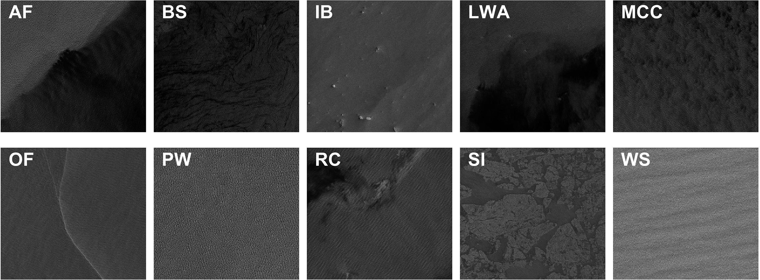
Figure 1 Description of the TenGeoP-SARwv dataset. Ten examples of defined geophysical phenomena: atmospheric fronts (AF); biological slicks (BS); icebergs (IB); low-wind areas (LWA); microconvective cells (MCC); oceanic fronts (OF); pure ocean waves (PW); rain cells (RC); sea ice (SI); and windstreaks (WS).

FIGURE 2

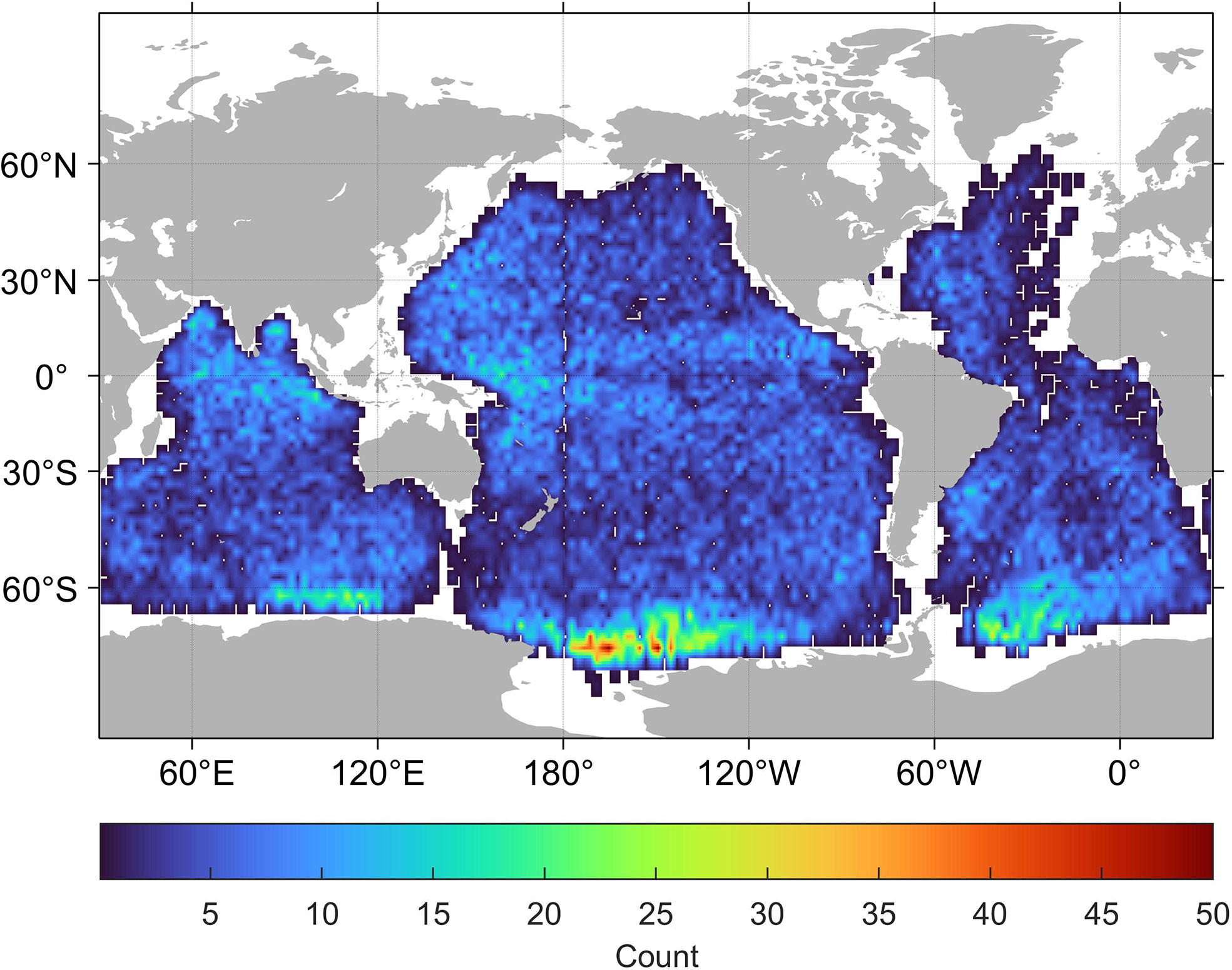
Figure 2 SAR data coverage under VV polarization in 2016. The color represents the number of WV images within each 5° by 5° spatial bin.

2.2 Kernel entropy component analysis

As the name implies, KECA attempts to select the most entropic components instead of variance-based or principal components in KPCA to extract features of interest. As is well known, the concept of Rényi quadratic entropy is as follows:

$\begin{array}{ll}H(p)=-\log {\displaystyle \int p^2(x)dx}& (1)\end{array}$

where p(x) denotes the probability density function. Equation (1) can be regarded as the measure of information derived from the given input images $X=\left[x_1,\dots ,x_N\right]$$(x_i\in {ℝ}^D)$

in KECA (Jenssen, 2009). Considering the monotonic property of logarithmic function, Equation (1) can be simplified as follows:

$\begin{array}{ll}V(p)={\displaystyle \int p^2(x})dx& (2)\end{array}$

Using a kernel $k_{\sigma }(x,x_t)$ of the Parzen window density estimator combined with the width coefficient σ (Jenssen, 2009), Equation (2) is converted to

$\begin{array}{ll}\begin{array}{l}V(p)\approx \widehat{V}(p)\\ =\frac{1}{N}{\displaystyle \sum _{x\in X}p(x)}\\ =\frac{1}{N}{\displaystyle \sum _{x_i\in X}\frac{1}{N}{\displaystyle \sum _{x_j\in X}{k}_{\sigma }(x_i,x_j)}}\\ =\frac{1}{N^2}{1}^{T}K1\end{array}& (3)\end{array}$

where $K=\left\{K_{ij}|K_{ij}=k_{\sigma }(x_i,x_j)\right\}$ is the kernel matrix and 1 is an N-dimensional vector containing all ones. Employing eigendecomposition (Jenssen, 2009)

$\begin{array}{ll}K=A{A}^T=\left(W{D}^{\frac{1}{2}}\right)\left(D^{\frac{1}{2}}{W}^T\right)& (4)\end{array}$

Equation (9) can be transformed into

$\begin{array}{ll}\widehat{V}(p)=\frac{1}{N^2}{\displaystyle \sum _{i=1}^N{\left(\sqrt{{\lambda }_i}{1}^T{\omega }_i\right)}^2}& (5)\end{array}$

where the eigenvalues ${\lambda }_1,\cdots ,{\lambda }_N$ corresponding to ${\omega }_1,\cdots ,{\omega }_N$ is reserved as the entropy estimate. In another word, KECA performs feature extraction not by the eigenvectors associated with the top N_c eigenvalues but by the axes contributing most to the Rényi entropy estimate $\widehat{V}(p)$ (Jenssen, 2009; Bai et al., 2020a). This can be concluded as the most distinct difference between KECA and KPCA (Jenssen, 2009).

2.3 KECANet for ocean SAR scene classification

In the interest of easy understanding for the reader, we first present the main flowchart of an ocean SAR scene classification based on KECA in Figure 3, whose main steps can be summarized as follows. 1) The SAR imagettes are preprocessed using a batch normalization technique and are then used as input into KECANet. 2) Noting that KECANet consists of multiple stages of successive convolutional layers and pooling layers, an approximation of KECA by the pivoted Cholesky decomposition (Harbrecht et al., 2012) is adopted for learning the filters to extract features in its convolutional layers. 3) The features of different imagettes are introduced to a final stage of spectral histogram (SH) encoding. Then, the output of classification results can be accomplished by the most naïve nearest neighbor classifier with cosine similarity scores. The internal structure of KECANet is also shown in Figure 4 for experimental reproduction. In the following sections, we describe the entirety of the process in detail.

FIGURE 3

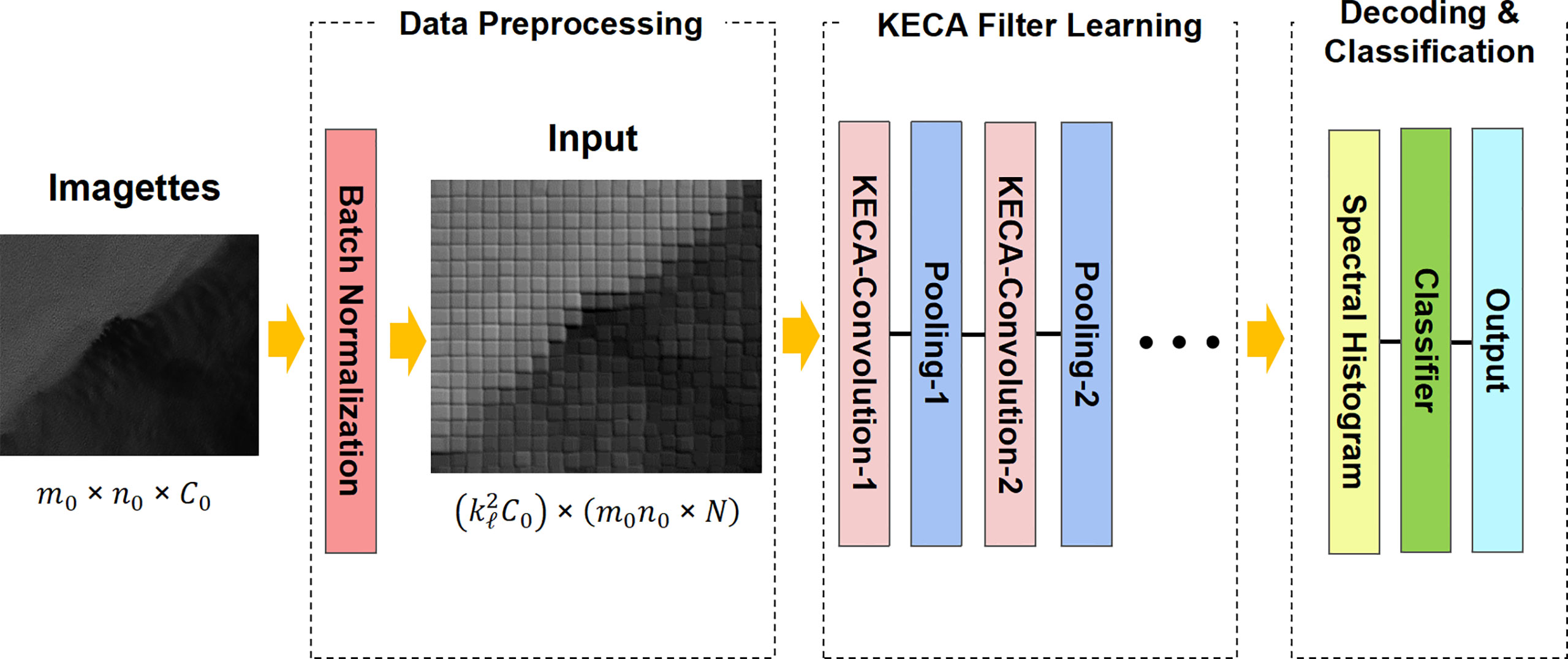
Figure 3 The workflow of ocean SAR scene classification using KECANet.

FIGURE 4

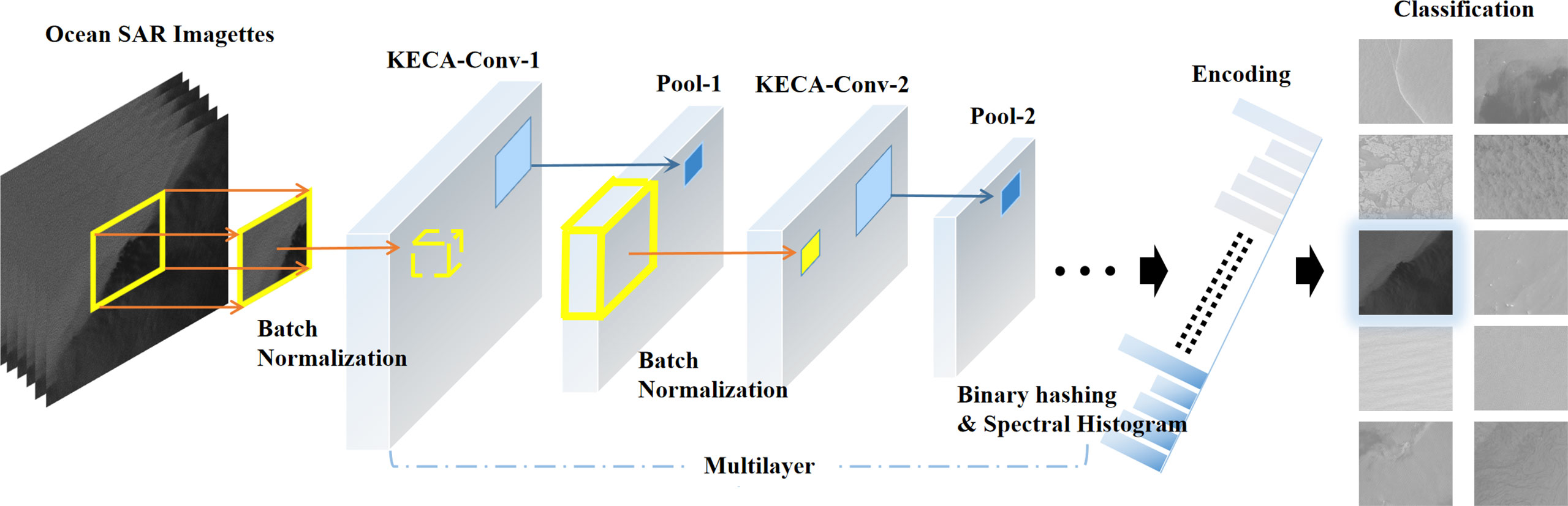
Figure 4 Architecture of the KECANet algorithm: batch normalization, multilayer convolution using KECA filters and mean pooling (nonlinearity), and SH feature encoding on layerwise feature maps.

2.3.1 Data preprocessing

Assuming that N ocean SAR imagettes ${\left\{X_i^{(0)}\in {ℝ}^{m_0\times n_0\times C_0}\right\}}_{i=1}^N$

derived from the TenGeoP-SARwv dataset penetrate deep into the ℓth layer of KECANet, where the channel C₀ = 1 denotes the grayscale input, the overlapping (stride- S_ℓ , S_ℓ = 1 adopted in our work) patches of k_ℓ × k_ℓ are extracted from each $X_i^{(0)}$ . We subtract batch normalization from each patch using the z-score technique and obtain a cluster of ${\left\{{\overline{X}}_i^{(0)}\in {ℝ}^{\left(k_{\ell }^2{C}_0\right)\times \left(m_0{n}_0\times N\right)}\right\}}_{i=1}^N$ , which is fed into the following chain of convolution and pooling operations.

2.3.2 KECA filter learning

${\left\{{\overline{X}}_i^{(0)}\in {ℝ}^{(k_{\ell }^2{C}_0)\times \left(m_0{n}_0\times N\right)}\right\}}_{i=1}^N$ D_ℓ -dimensional RKHS using the Equations (3)–(5). Thereafter, the ℓ th layer can obtain the feature maps from the preceding (ℓ−1) th layer

$\begin{array}{ll}{\overline{X}}_i^{(\ell )}=\beta \left({\overline{X}}_i^{(\ell -1)}\ast W^{(\ell )}\right)\in {ℝ}^{m_{\ell -1}\times n_{\ell -1}\times C_{\ell }}& (6)\end{array}$

where * represents a convolution operator and β(·) denotes the nonlinear mean pooling with a pooling window of θ_ℓ × θ_ℓ such that m_ℓ = (m_ℓ−1−θ_ℓ)/s_ℓ + 1 and $n_{\ell }=(n_{\ell -1}-{\theta }_{\ell })/s_{\ell }+1$. $W^{(\ell )}\in {ℝ}^{(k_{\ell }^2{C}_{\ell -1})\times C_{\ell }}$ is defined as the layerwise filter ensemble with c_ℓ KECA filters prelearned from the (ℓ−1) th layer. However, there are several limitations in directly using the KECA algorithm, e.g., too many computations when calculating the kernel matrix (as many as O(N³) , where N is often more than 1K) and low efficiency of the representation as compared to deep learning methods (Bengio and LeCun, 2007). Hence, we provide an efficient algorithm (please refer to Algorithm 1) to obtain a low-rank approximation of the kernel matrix, while effectively maintaining the outstanding performance of KECA. The key to the mathematical analysis of Algorithm 1 is illustrated as follows. Let $K_i^{(\ell )}\in {ℝ}^{(m_{\ell }{n}_{\ell })\times (m_{\ell }{n}_{\ell })}$ be a kernel matrix derived from ${\overline{X}}_i^{(\ell )}$. In order to save time and memory when obtaining $K_i^{(\ell )}$ , on the basis of Equation (4), we carry out the eigendecomposition on a smaller feature space, i.e., of size $r_{\ell }\ll m_{\ell }{n}_{\ell }$ . Then, we expand the results back up to $m_{\ell }{n}_{\ell }$ dimensions. In other words, our intention here is to seek a Nyström-type low-rank approximation ${\tilde{K}}_i^{(\ell )}$ of $K_i^{(\ell )}$ that satisfies the approximation error $\Vert E_i^{(\ell )}\Vert =\Vert K_i^{(\ell )}-{\tilde{K}}_i^{(\ell )}\Vert \le \epsilon$. Finally, after substituting ${\tilde{K}}_i^{(\ell )}$ into Equations (4) and (5), we can obtain the KECA learning filters $w^{(\ell )}$ from the $(\ell -1)$ th layer for feature extraction.

Lemma 1. The low-rank approximation ${\tilde{K}}_i^{(\ell )}$ derived from the Algorithm 1 satisfies $\Vert E_i^{(\ell )}\Vert =\Vert K_i^{(\ell )}-K_i^{(\ell )}\Vert \le \epsilon$, where ϵ denotes a minimum value.

Proof of Lemma 1. For simplicity, let $\tilde{K}$ and $K_i^{(\ell )}$ represent ${\tilde{K}}_i^{(\ell )}$ and K with N_ℓ = m_ℓ n_ℓ , respectively. Considering that ${\tilde{K}}_j$ obtained in the j th iteration is a positive semidefinite matrix (Harbrecht et al., 2012), ${\tilde{K}}_j$ can be decomposed by the Cholesky technique (Harbrecht et al., 2012; Zhou, 2015).

$\begin{array}{ll}{\tilde{K}}_j=K^{N_l\times j}{\left(K^{j\times j}\right)}^{-1}{\left(K^{N_1\times j}\right)}^T=P_j{\left(P_j\right)}^T& (7)\end{array}$

Without loss of generality, we assume

$\begin{array}{ll}{\tilde{K}}_{j+1}=K^{N_l\times (j+1)}{\left(K^{\left(j+1\right)\times \left(j+1\right)}\right)}^{-1}{\left(K^{N_1\times \left(j+1\right)}\right)}^T=P_{j+1}{\left(P_{j+1}\right)}^T& (8)\end{array}$

On the basis of Cholesky factorization:

$\begin{array}{ll}{K}^{j\times j}=L_j{L}_j^T& (9)\end{array}$

where L_j is a lower triangular matrix. Then, substituting Equation (9) into Equation (7), we obtain

$\begin{array}{ll}{P}_j=K^{N_l\times j}{\left(L_j\right)}^{-T}& (10)\end{array}$

Motivated by the pivoted Cholesky decomposition (Harbrecht et al., 2012; Zhou, 2015), let

$\begin{array}{ll}{K}^{\left(j+1\right)\times \left(j+1\right)}=\left[{}_{K_t^{j\times 1}}^{K^{j+1}}{}_{K_{tt}}{}^{K_t^{j\times 1}}\right]={\left(L_{j+1}\right)}^T{L}_{j+1}& (11)\end{array}$

where $K_t^{j\times 1}={\left(K_{1t},\cdots ,K_{jt}\right)}^T$ , i.e., the tth kernel column. Using Equations (9)–(11), we can obtain Step 4 in Algorithm 1:

$\begin{array}{ll}{L}_{j+1}=[{}_{u^T}^{L_j}{}_{\mu }{}^0]& (12)\end{array}$

where $u={(L_j)}^{-1}{K}_t^{j\times 1}$ is exactly the tth column of $P_j$ and $\mu ={\sqrt{K}}_{tt}-u^{T}u$ . Let

$\begin{array}{ll}{P}_{j+1}=[P_j{p}_j]& (13)\end{array}$

On the basis of Equations (8) and (12), we obtain

$\begin{array}{ll}{P}_{j+1}=K^{N_l\times \left(j+1\right)}{L}_{j+1}^{-T}=[P_j{\mu }^{-1}\left(K_t^{N_l\times 1}{L}_{j}u\right)]& (14)\end{array}$

Therefore, the approximation error in iterations is

$\begin{array}{ll}{E}_{j+1}={\tilde{K}}_j-{\tilde{K}}_{j+1}=P_j{\left(P_j\right)}^T=E_j-p_j^2& (15)\end{array}$

which means that the error is monotonically decreasing until it meets the error tolerance ϵ.

For convenient computing, the trace norm is chosen in Step 9 as the error measurement in Algorithm 1. □

ALGORITHM 1

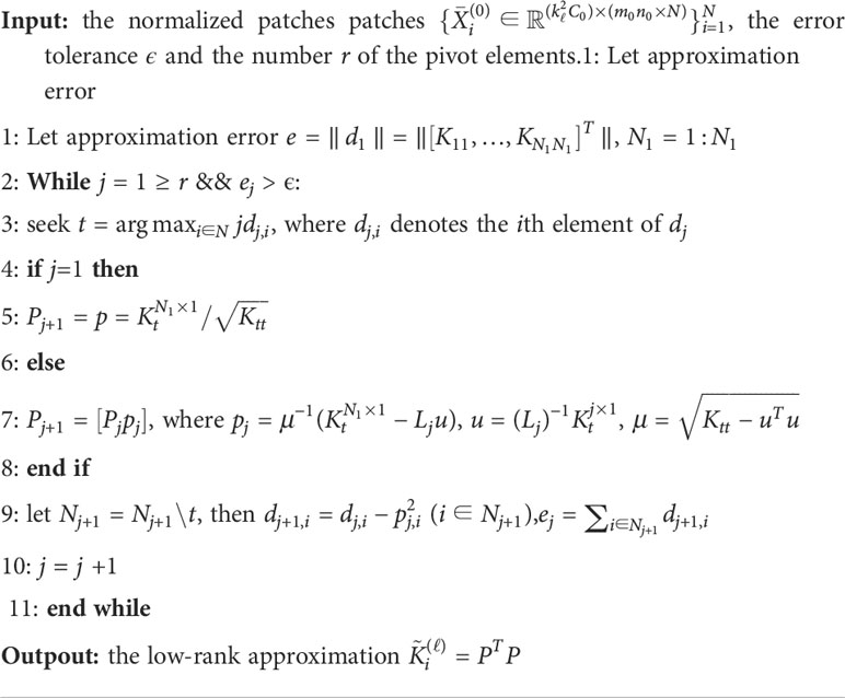
Algorithm 1

2.3.3 Encoding and classification

After the aforementioned stages, involving the convolutional, mean pooling, and KECA layers, a binary hashing similar to PCANet"s is employed in KECANet to compute the block-wise histograms in encoding stage. Specifically, we first binarize the outputs of $(X{}^{\left(\ell -1\right)}\ast W^{(\ell )})\in {ℝ}^{m_{\ell -1}\times n_{\ell -1}\times C_{\ell }}$ before pooling. The hashed feature maps are divided into $C_{\ell }/C_{\lambda }$ (pre-fixed $C_{\lambda }$ to 8 after fine tuning) different sets and each set is encoded with a $C_{\ell }$ bit integer. Secondly, we can obtain

$\begin{array}{ll}{S}_t^{\left(\ell \right)}={\displaystyle \sum _{c=1}^{C_{\lambda }}unit\left({\overline{X}}^{\left(\ell -1\right)}\ast {\left(W^{\left(\ell \right)}\right)}_{C_{\lambda }\left(t-1\right)+c}\right)}{2}^{c-1}{t}_{}& (16)\end{array}$

where $t=1,\dots ,H_{\ell }$ and $unit(\cdot )$ represents the unit step function (Low et al., 2017). Thirdly, $S_t^{\left(\ell \right)}$ is clustered into $B_{\ell }$ nonoverlapping blocks, each of whom is histogrammed into $2^{C_{\lambda }}$ bins. Thus, in each layer, $H_{\ell }{B}_{\ell }$ blockwise histograms are cascaded to form the final feature vector of the input SAR imagette. Finally, the feature vectors derived from KECANet can be trained by the most naïve nearest neighbor classifier with Cosine similarity scores and achieve ocean scene recognition.

2.4 Computational complexity

In the data preprocessing stage, the main cost of z-score normalization is $O\left(N{m}_0{n}_0\right)$ computations. In the KECA filter learning stage, the complexity of Algorithm 1 is $O\left(r^{2}N\right)$. This is very efficient as compared to O(N³), which is required by the conventional kernel method ($r\le 9$). The eigendecomposition of approximation kernel matrix needs $O\left(D_{\ell }^3\right)$ computations. The cost of mapping the patches to the RKHS space is $O\left(D_{\ell }^{2}N\right)$. In the final stage, the binary hashing and block-wise histograms require $O\left(2D_{\ell }N\right)$ and $O\left(H_{\ell }{B}_{\ell }{D}_{\ell }N{\log }_2\right)$. Considering $N\gg \max \left(m_{\ell },n_{\ell },D_{\ell },H_{\ell },B_{\ell }\right)$, the overall cost of KECANet is presented as follows:

$\begin{array}{ll}O\left({\displaystyle \sum _{\ell =1}^{L}N{m}_{\ell }{n}_{\ell }+{\displaystyle \sum _{\ell =1}^{L}N\left(r^2+D_{\ell }^2\right)}}\right)& (17)\end{array}$

which can be simplified as (due to $D_{\ell }\gg r$ )

$\begin{array}{ll}O\left({\displaystyle \sum _{\ell =1}^{L}N\left(D_{\ell }^2+m_{\ell }{n}_{\ell }\right)}\right)& (18)\end{array}$

Considering that the complexity of a two-stage PCANet is $O({{\sum }_{\ell =1}^2{\displaystyle N(m_{\ell }{n}_{\ell })}}^2)$ (Chan et al., 2015) and $D_{\ell }/m_{\ell }{n}_{\ell }\ll 1$ for SAR imagery, the complexity of KECANet is lower than PCANet, which requires far fewer computations than CKNs (Mairal et al., 2014; Mohammadnia-Qaraei et al., 2018; Qaraei et al., 2021). In the next section, we demonstrate the potential and performance of KECANet in detail.

3 Experiment and results

This section starts with a detailed ablation study to analyze the contributions of deep learning architecture and the pivoted Cholesky decomposition to a conventional KECA method. Afterward, considering that deep kernelized methods are greatly impacted by the number of layers and the width coefficient, we implemented a sensitivity analysis on these two important coefficients using the TenGeoP-SARwv dataset. Then, another experiment on noise-filled SAR imagettes was also performed to test the noise robustness of KECANet. To further validate the model performance, a geophysical map of sea ice in Antarctica, as detected by KECANet, is analyzed and compared with the global gridded product. Finally, we compared KECA with several different methods and presented state-of-the-art results for undertaking the task of ocean SAR scene auto-classification. For the training strategies in this section, we adopted the set proposed by Wang et al. (2019b). A total of 320 imagettes per class (N = 320) were randomly chosen as the input dataset from the annotated TenGeoP-SARwv dataset separated by WV1 and WV2. Notably, the size of the input was relatively small. Moreover, 70% and 30% of the dataset were selected as the training and testing subsets, respectively. All of the experiments without data augmentation were implemented by MATLAB R2021b on a server with GN7.2XLARGE32 processors, 32 GB memory, and a Windows Server 2016 operating system. All results were averaged over 10 runs. The reported values of the recall (R), precision (P), and F-score (F) were averaged over 10 repeated experiments. The values of these three parameters were all expected to approach one (Wang et al., 2019b). KECANet was implemented using the parameter configuration shown in Table 1.

TABLE 1

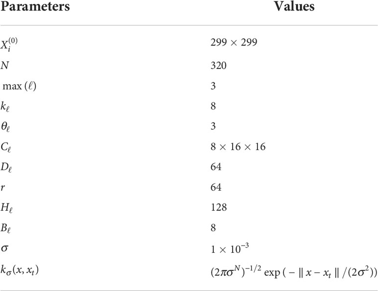
Table 1 KECANet parameter configuration for the TenGeoP-SARwv database.

3.1 Ablation study

Table 2 shows the classification results of various variants of KECA on the test set of the TenGeoP-SARwv dataset. Noting that KECA is the original method (Jenssen, 2009), KECANet-1 and KECANet-2 denote a KECA, which has penetrated deep into the 1st and 2nd layers, respectively, without using the accelerating technique of the pivoted Cholesky decomposition. Low-rank KECANet-1 and Low-rank KECANet-2 integrate the deep learning architecture and the accelerating technique with the conventional KECA (Jenssen, 2009). Table 2 empirically validates the effectiveness of using deep learning methods, considering that KECANet-1 improves the averaged classification result of KECA by 6.48%, 23.25%, and 12.96% in R, P, and F statistics, respectively. Table 2 also shows that using the accelerating technique can significantly reduce computing time and memory since KECANet-2 was so prone to exhausting its memory that it severely impeded its functionality. Compared to the original KECA, we progressively improved classification accuracy in R, P, and F statistics by 46.21%, 44.99%, and 46.53%, respectively.

TABLE 2

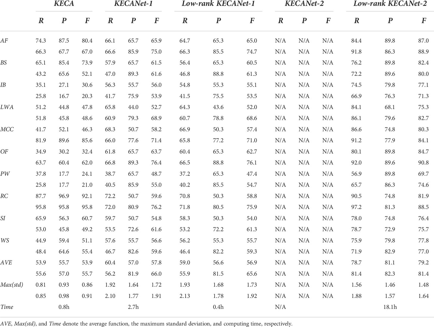
Table 2 Ablation Study of KECA on WV1 (upper) and WV2 (lower) imagette recognition (%).

3.2 Impact of the number of layers

We evaluated KECANet"s performance on the selected dataset using different numbers of layers. The KECA filter ensemble $C_{\ell }$ of $8\times 8\times 16\times 16$ was selected in layer 4. Table 3 illustrates the overall performance for multilayer KECANet. It can be observed that KECANet"s average performance regarding R, P, and F increased from 58.99%, 56.63%, and 56.87% in layer 1, to 86.40%, 84.73%, and 84.95% in layer 4. Considering a tradeoff between computing time and classification performance (the advantage of KECANet-4 is almost negligible as compared to KECANet-3), the maximum number of layers, i.e., $\max \left(\ell \right)=3$, was adopted in this study. KECANet-3 is denoted as KECANet for simplicity in the rest of the article unless otherwise stated.

TABLE 3

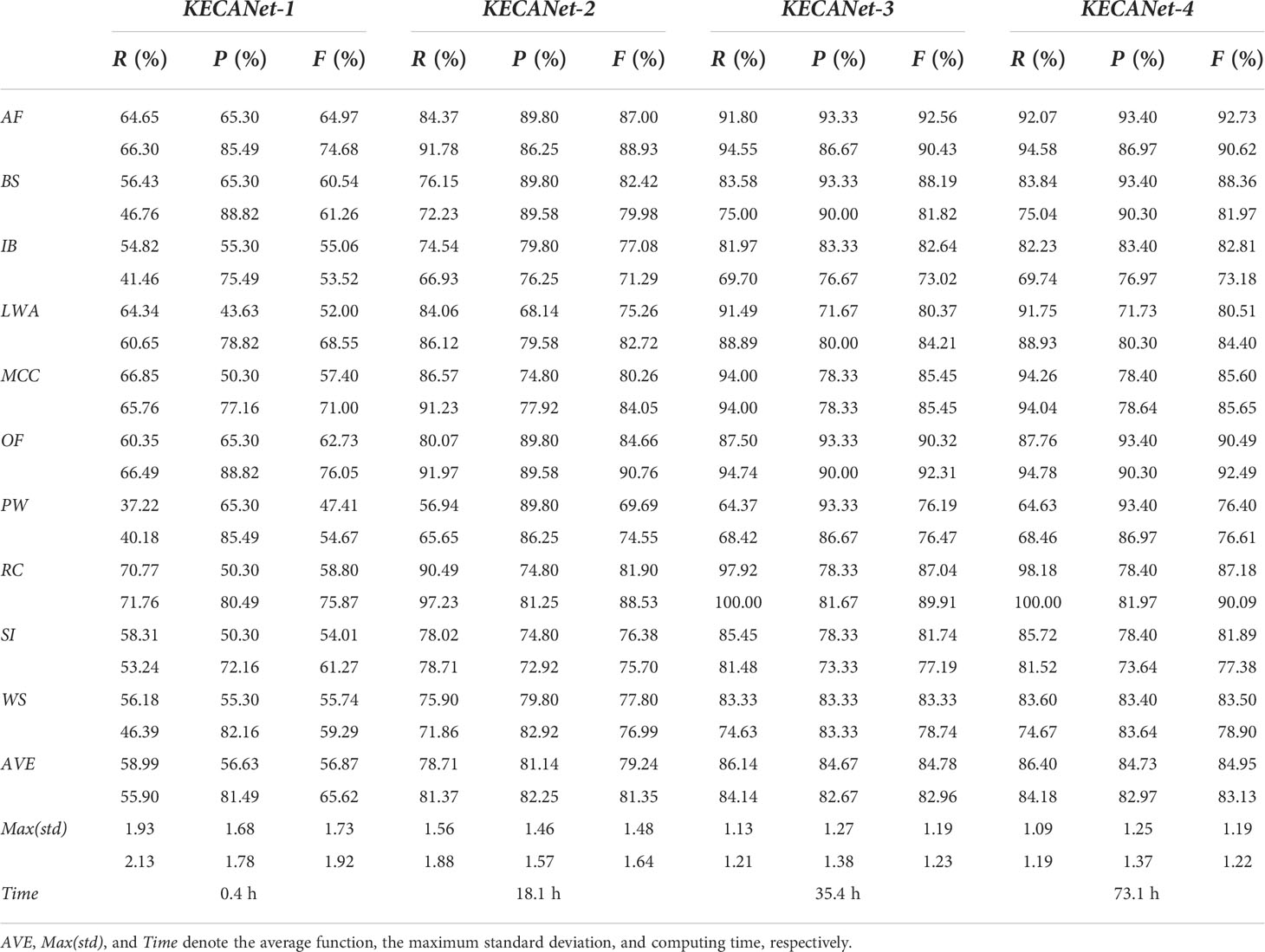
Table 3 Classification performance (%) in WV1 (upper) and WV2 (lower) imagette recognition for KECANet using different layers.

3.3 Impact of the width coefficient

The width coefficient, also known as the kernel width σ , plays a role in kernel-based methods (Bai et al., 2019; Bai et al., 2020a). We evaluated the impact of the width of KECANet on the selected dataset. The average results of classifying 10 geophysical phenomena are shown in Figure 5. The width coefficients of three layers were the same and ranged from $1\times {10}^{-4}$ to 1. The results show that the classification performances increase significantly as a result of properly choosing the width coefficient. Therefore, $1\times {10}^{-3}$ was adopted in this study. More details are shown in Table 4.

FIGURE 5

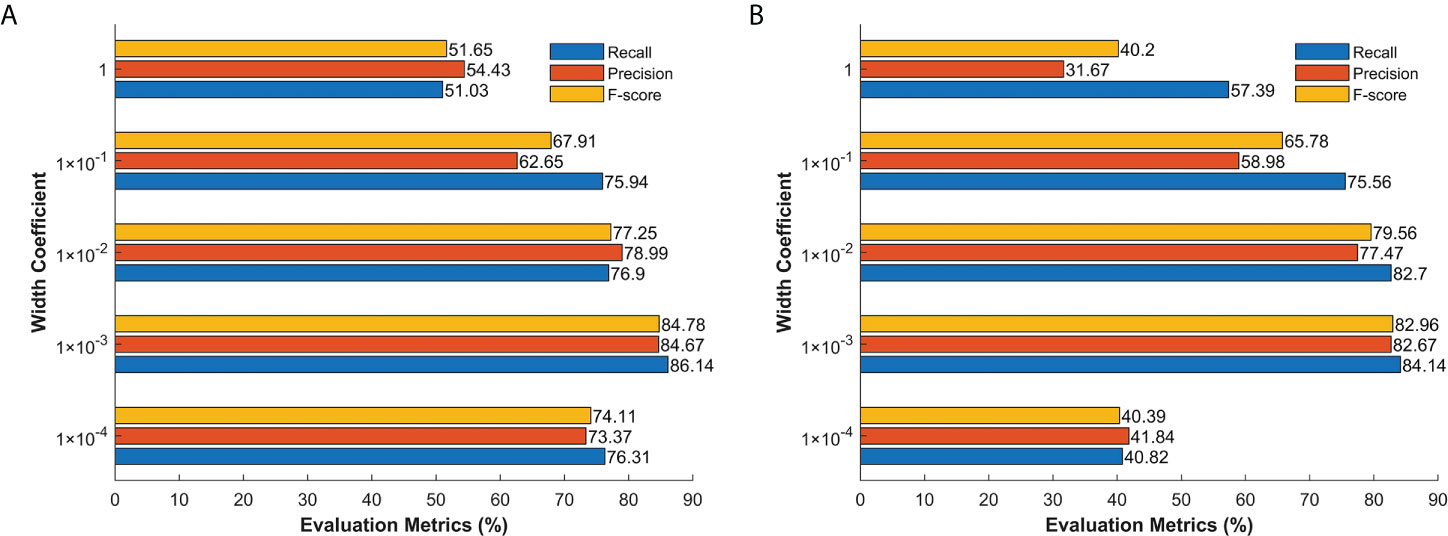
Figure 5 Average classification performance in WV1 (A) and WV2 (B) imagette classification of KECANet equipped with different width coefficients.

TABLE 4

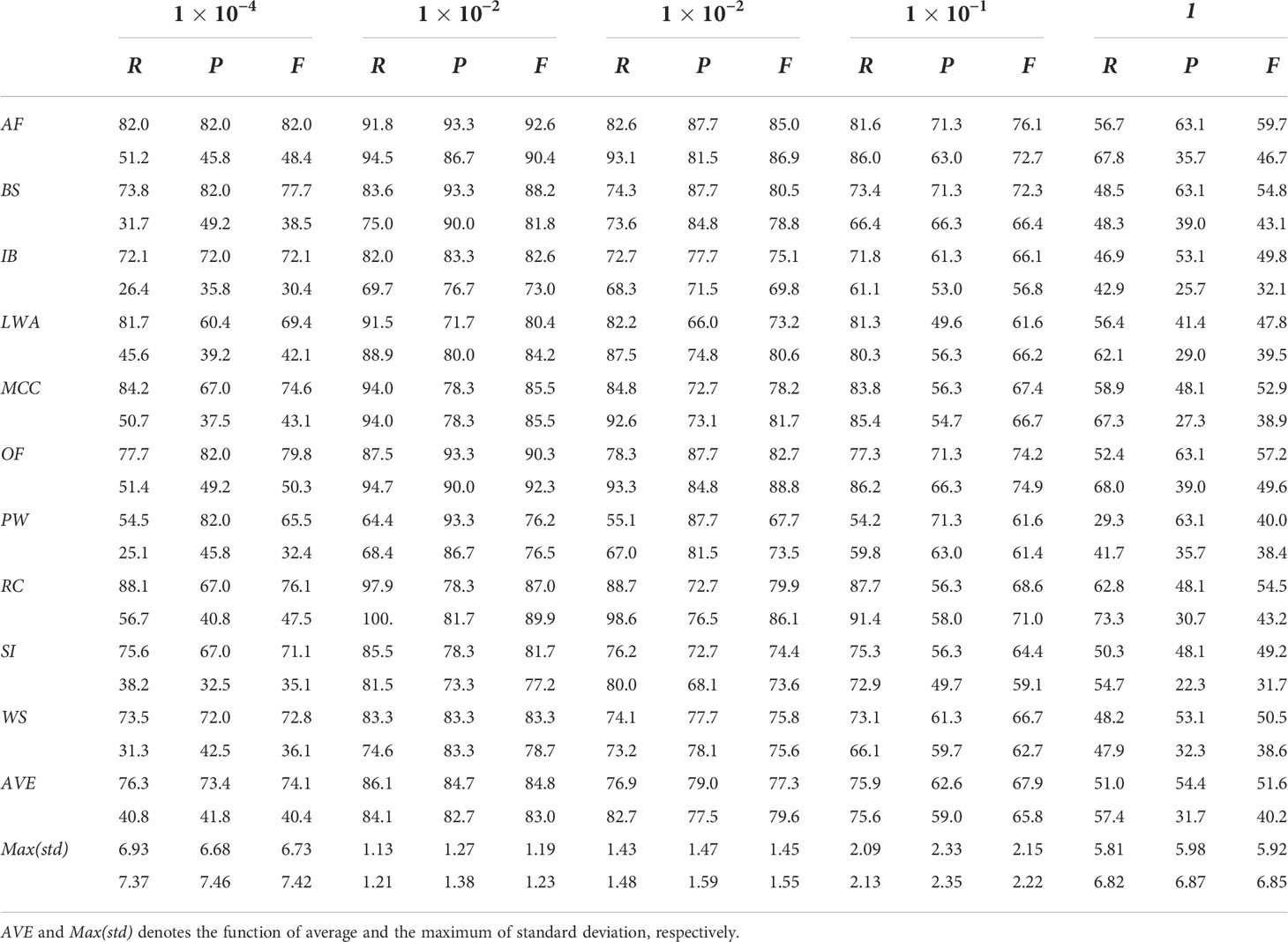
Table 4 Classification performance (%) in WV1 (upper) and WV2 (lower) imagette recognition of KECANet equipped with different width coefficients.

3.4 KECANet for denoising

In this subsection, we evaluate the noise robustness of KECANet. We randomly selected 200 imagettes of each oceanic phenomenon and added block noise to the input datasets. All noise insertions accounted for 0.01 to 0.15 of the image area and were located within a rectangle with randomly distributed positions (please refer to Figure 6). Thus, we established a new gallery split into two subsets for the classification experiment. One subset was used for training, including 140 noisy imagettes and 84 noise-free imagettes per class. The other subset contained the remainder for testing. We ran this process 10 times. Table 5 shows the classification results versus those derived from KECANet on the original dataset. By comparative analysis, we can conclude that KECANet can provide relatively acceptable robustness in SAR data denoising, considering it obtained more than 82% in R, P, and F statistics, even though the classification performances deteriorated by about 1–2% in calibration metrics.

FIGURE 6

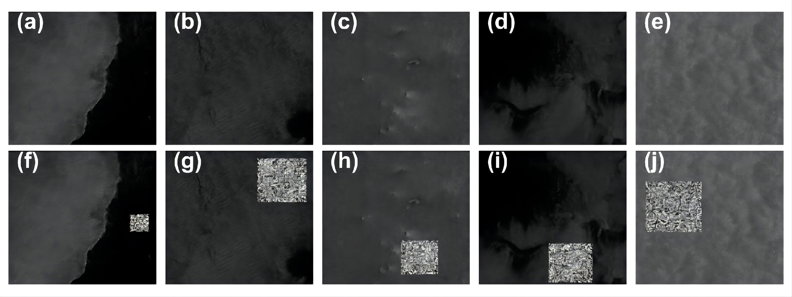
Figure 6 The first row (A–E) presents randomly selected 5 imagettes in the TenGeoP-SARwv dataset. The second row (F–J) show the associated noisy imagettes.

TABLE 5

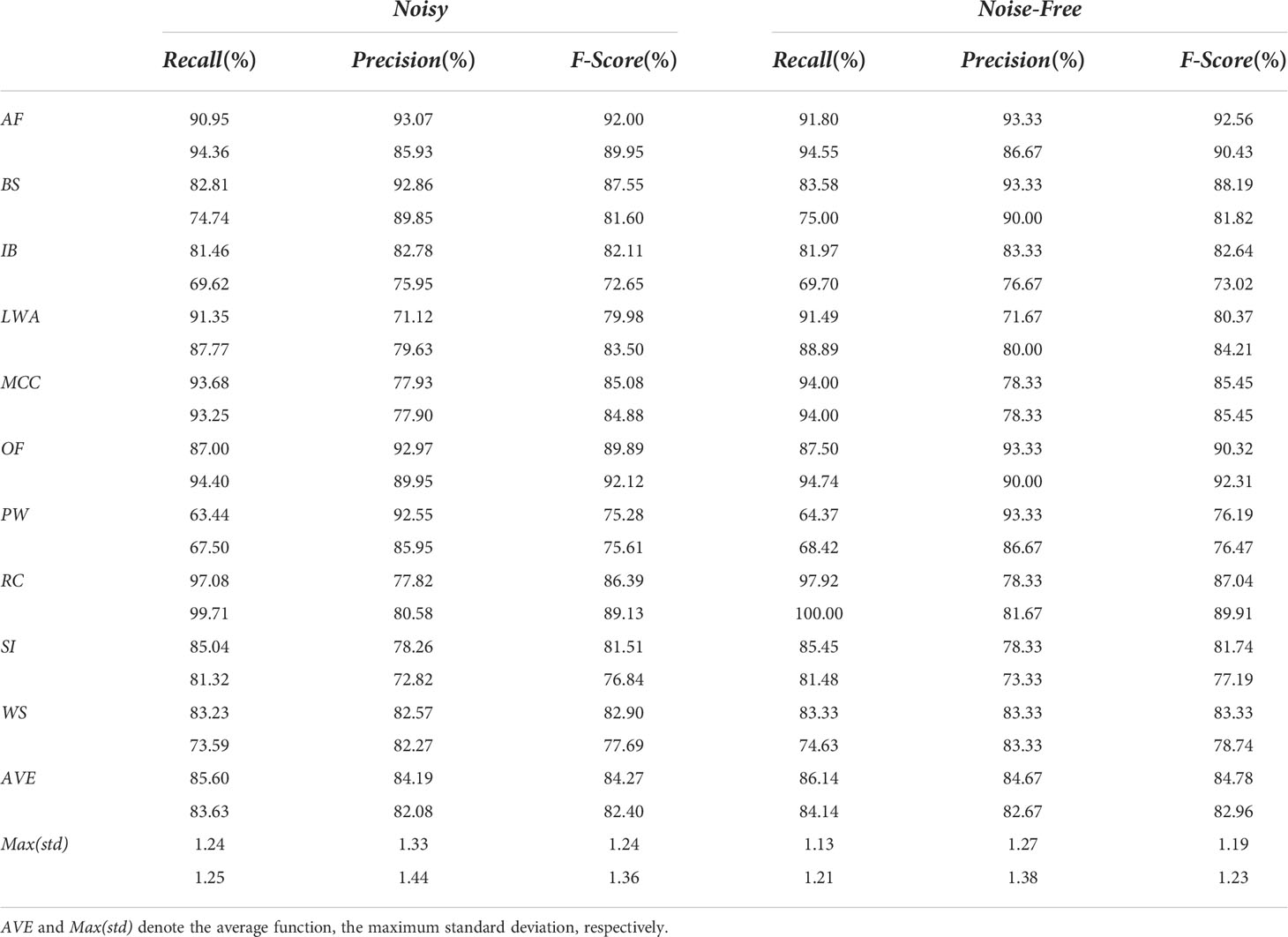
Table 5 Classification performance (%) in WV1 (upper) and WV2 (lower) imagette recognition for KECANet using noisy and noise-free datasets.

3.5 A geophysical application

To further verify the credibility capabilities of KECANet, the deep learning method was applied to all SAR imagettes from January to December 2016 in the TenGeoP-SARwv dataset. We examined the geophysical map of detected sea ice comparable to the NOAA/NSIDC Climate Data Record of Passive Microwave Sea Ice Concentration (Version 4, CDRPM-SIC) (Meier et al., 2021). From January to December 2016, nearly 5% of SAR imagettes are classified as SI by KECANet. More than 90% of them are distributed near Antarctica due to the satellite coverage and perennial low temperatures around the polar Southern Ocean. The mapping of classified SI occurrence in Figures 7A–D shows a clear seasonal variability, increasing from early April to a maximum in the Antarctic winter period (from June to October) before decreasing after that. Specifically, in the austral winter (please refer to Figures 7B, C), there is abundant sea ice from 20°E to 60°W and from 100°W to 150°E. Most of it is distributed around Antarctica and poleward of 60°S, or even 54°S. As can be seen in Figure 7D, the summer period sea ice significantly decreases compared to the winter, especially from 120°W to 180°. Sea ice concentration data from the National Snow and Ice Data Center (NSDIC) are also compared in Figures 7E–H. Although the CDRPM-SIC aims at the gridded polar SIC product leading to greatly different resolutions between the first and the second rows of Figure 7, most areas of higher SI occurrence, as detected by KECANet, mirror the high SIC areas. For example, this is especially true for the sea ice extent that expands to the north of 60°S (20°E to 60°W) in the April–June season (see Figures 7B, F). This agreement is another measure of the capability of KECANet as an ocean SAR scene classification tool.

FIGURE 7

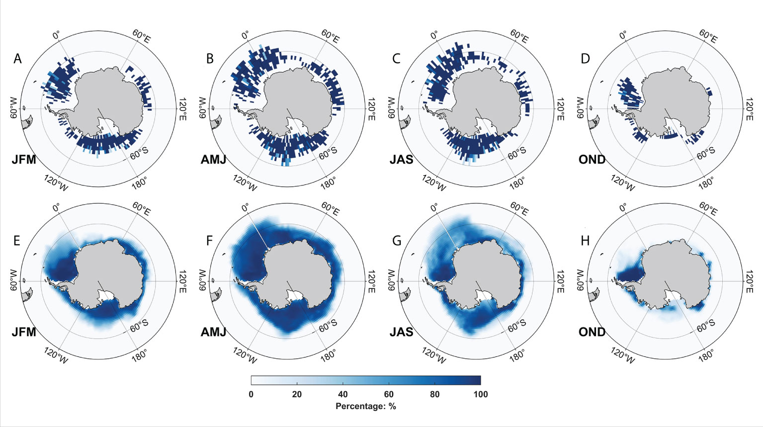
Figure 7 Sea ice around the Antarctica from January 2016 to December 2016. Sea ice coverage detected by KECANet in seasons: January-February-March (JFM), April-May-June (AMJ), July-August-September (JAS) and October-November-December (OND) are shown in (A-D) with color denoting the occurrence percentage in 2° × 2° boxes. (E-H) show the mean sea ice concentration from the NSIDC monthly product.

3.6 Comparison with state-of-the-art methods

In this subsection, we present the averaged results for the task of ocean SAR scene classification using several well-known models over 10 runs for comparison. The same training strategies with KECANet were adopted here. CMwv (Wang et al., 2019b), a CNN-type model, was selected as the baseline as a result of its notable ability in ocean SAR scene classification. Additionally, CKN, as proposed by Mairal et al. (2014) (denoted Gauss-CKN), and RNPCANet (Qaraei et al., 2021) were also employed as state-of-the-art representative models for CKN. We also selected PCANet (Chan et al., 2015) for comparison considering its impressive results in face recognition tasks. As proposed in (Qaraei et al., 2021), for PCANet and RNPCANet, the number of layers was set to 2. The size of both filters and blocks was 7 × 7 and the overlap ratio of the blocks was 0.5. The parameter set for Gauss-CKN was the default set in the code provided by Dr. Mairal, which is available at https://lear.Inrialpes.fr/people/mairal/solaris/software.html. CMwv was fine-tuned as suggested in (Wang et al., 2019b). The performances of the aforementioned methods are summarized in Figure 8 including average recall, precision, and F-score statistics. More details can be found in Table 6. Our observations are as follows:

1. KECANet yielded the best classification accuracy considering that F-score statistics are a combined index of both precision and recall statistics, when no data augmentation is applied. This is because the feature extracted by KECA optimally reveals the structure corresponding to the maximum Rényi entropy of the original SAR data and encodes the discriminant information. Overall, the average recall, precision, and F-score values obtained with KECANet were 86.1% (84.1%), 84.7% (82.7%), and 84.8% (83.0%) higher than the other methods when applied in WV1 (WV2) imagette classification, excepting the recall achieved with Gauss-CKN on WV2;

2. Although KECANet performs marginally better than Gauss-CKN, Gauss-CKN requires more computational resources and time than KECANet;

3. The classification performances of CKN models (i.e., KECANet, Gauss-CKN, and RNPCANet) are superior to those of CNN-type models (i.e., PCANet and CMwv) on ocean SAR imagettes.

FIGURE 8

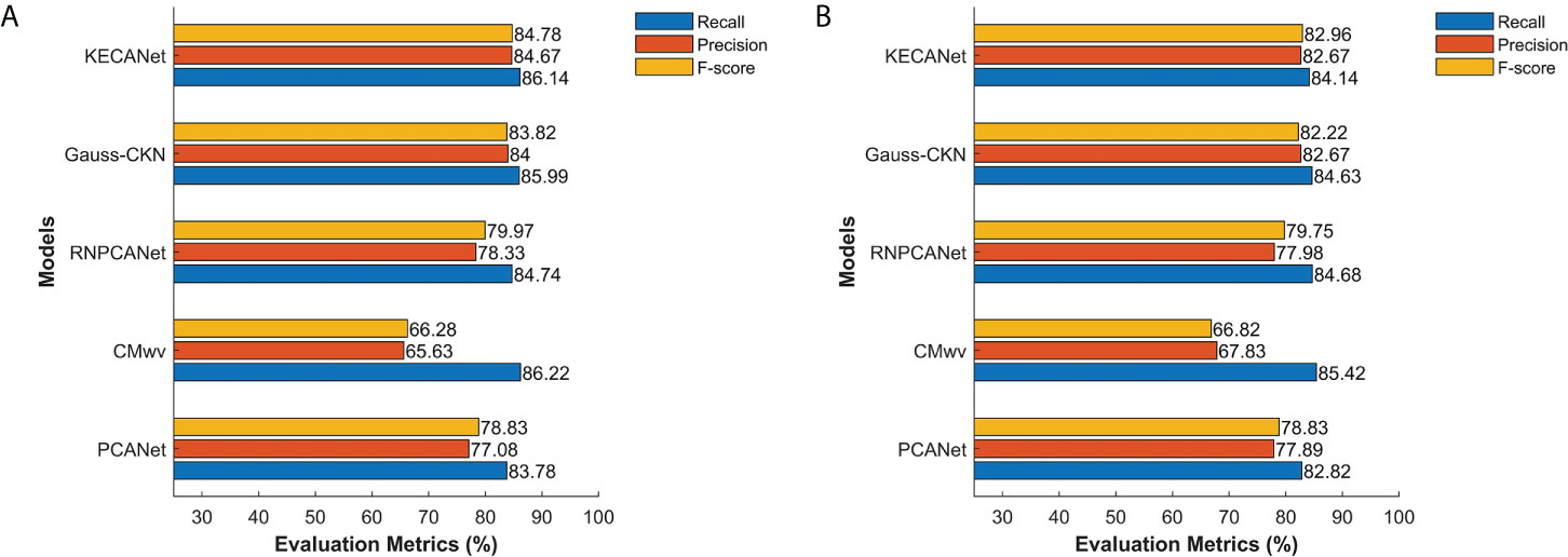
Figure 8 Average classification performance in WV1 (A) and WV2 (B) imagette classification of different methods.

TABLE 6

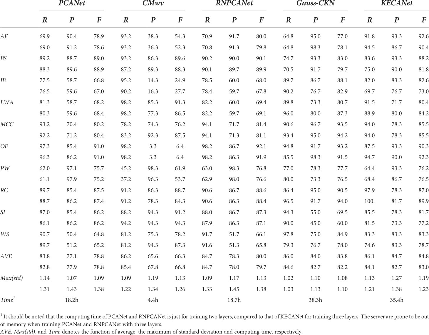
Table 6 Classification performance (%) in WV1 (upper) and WV2 (lower) imagette recognition of different methods.

4 Discussion and conclusions

This paper proposes a new deep learning method, KECANet, for combining kernel entropy component analysis with the pivoted Cholesky decomposition and convolutional kernel networks. Through an ablation study, we demonstrate that mixing these three concepts is fruitful. We also achieved an acceptable performance compared with several conventional and state-of-the-art models (e.g., PCANet, RNPCANet, CMwv, etc.) on a high-quality SAR dataset called TenGeoP-SARwv, which has a simple architecture and limited labeled samples. Although KECANet has shown potential for automated ocean SAR scene classification, various challenges related to our model remain open for future research. One such challenge concerns the use of GPU acceleration technology to improve classification task efficiency. Another involves leveraging the theoretical interpretation of our convolutional kernel networks to better understand network function.

Data availability statement

The original contributions presented in the study are included in the article/supplementary material. Further inquiries can be directed to the corresponding author.

Author contributions

MM designed and conceived the experiments; CB and HY implemented the experiments; LQ analyzed the data; CB and SZ wrote the paper. All authors contributed to the article and approved the submitted version.

Funding

This work was supported by the National Natural Science Foundation of China (Grant No. 42106200).

Conflict of interest

The authors declare that the research was conducted in the absence of any commercial or financial relationships that could be construed as a potential conflict of interest.

Publisher's note

All claims expressed in this article are solely those of the authors and do not necessarily represent those of their affiliated organizations, or those of the publisher, the editors and the reviewers. Any product that may be evaluated in this article, or claim that may be made by its manufacturer, is not guaranteed or endorsed by the publisher.

References

Bai L., Han Z., Ren J., Qin X. (2020b). Research on feature selection for rotating machinery based on supervision kernel entropy component analysis with whale optimization algorithm. Appl. Soft Comput. 92, 106245. doi: 10.1016/j.asoc.2020.106245

CrossRef Full Text | Google Scholar

Bai C., Zhang R., Xu Z., Cheng R., Jin B., Chen J. (2019). L1-norm-based kernel entropy components. Pattern Recognit. 96, 106990. doi: 10.1016/j.patcog.2019.106990

CrossRef Full Text | Google Scholar

Bai C., Zhang R., Xu Z., Jin B., Chen J., Zhang S., et al. (2020a). Kernel low-rank entropic component analysis for hyperspectral image classification. IEEE J. Sel. Top. Appl. Earth Obs. Remote Sens. 13, 5682–5693. doi: 10.1109/jstars.2020.3024241

CrossRef Full Text | Google Scholar

Bao S., Meng J., Sun L., Liu Y. (2020). Detection of ocean internal waves based on faster r-CNN in SAR images. J. Oceanol. Limnol. 38, 55–63. doi: 10.1007/s00343-019-9028-6

CrossRef Full Text | Google Scholar

Bengio Y., LeCun Y. (2007). Scaling learning algorithms towards AI. in Large-Scale Kernel Mach. (Boston, America: MIT Press): 34, 1–41.

Google Scholar

Bioresita F., Puissant A., Stumpf A., Malet J. P. (2018). A method for automatic and rapid mapping of water surfaces from sentinel-1 imagery. Remote Sens. 10, 217. doi: 10.3390/rs10020217

CrossRef Full Text | Google Scholar

Bjerreskov K. S., Nord-Larsen T., Fensholt R. (2021). Classification of nemoral forests with fusion of multi-temporal sentinel-1 and 2 data. Remote Sens. 13, 950. doi: 10.3390/rs13050950

CrossRef Full Text | Google Scholar

Bo L., Sminchisescu C. (2009). Efficient match kernel between sets of features for visual recognition. Adv. Neural Inf. Process. Syst. 22, 1–9.

Google Scholar

Bottou L. (2012). “Stochastic gradient descent tricks,” in Neural networks: Tricks of the trade. Eds. Montavon G., Orr G. B., Müller K. R. (Berlin/Heidelberg, Germany: Springer), 421–436.

Google Scholar

Chan T. H., Jia K., Gao S., Lu J., Zeng Z., Ma Y. (2015). PCANet: a simple deep learning baseline for image classification? IEEE Trans. Image Process. 24, 5017–5032. doi: 10.1109/tip.2015.2475625

PubMed Abstract | CrossRef Full Text | Google Scholar

Clausi D. A. (2001). Comparison and fusion of co-occurrence, gabor and MRF texture features for classification of SAR sea-ice imagery. Atmos. Ocean 39, 183–194. doi: 10.1080/07055900.2001.9649675

CrossRef Full Text | Google Scholar

Du Y., Song W., He Q., Huang D., Liotta A., Su C. (2019). Deep learning with multi-scale feature fusion in remote sensing for automatic oceanic eddy detection. Inf. Fusion 49, 89–99. doi: 10.1016/j.inffus.2018.09.006

CrossRef Full Text | Google Scholar

Franz K., Roscher R., Milioto A., Wenzel S., Kusche J. (2018). Ocean eddy identification and tracking using neural networks, Proceedings of the IGARSS 2018 IEEE International Geoscience and Remote Sensing Symposium, Valencia, Spain. 6887–6890 (IEEE). doi: 10.1109/IGARSS.2018.8519261

CrossRef Full Text | Google Scholar

Gao F., Dong J., Li B., Xu Q. (2016). Automatic change detection in synthetic aperture radar images based on PCANet. IEEE geosci. Remote Sens. Lett. 13, 1792–1796. doi: 10.1109/lgrs.2016.2611001

CrossRef Full Text | Google Scholar

Gomez-Chova L., Jenssen R., Camps-Valls G. (2011). Kernel entropy component analysis for remote sensing image clustering. IEEE Geosci. Remote Sens. Lett. 9, 312–316. doi: 10.1109/lgrs.2011.2167212

CrossRef Full Text | Google Scholar

Gommenginger C., Chapron B., Hogg A., Buckingham C., Fox-Kemper B., Eriksson L., et al. (2019). SEASTAR: A mission to study ocean submesoscale dynamics and small-scale atmosphere-ocean processes in coastal, shelf and polar seas. Front. Mar. Sci. 6. doi: 10.3389/fmars.2019.00457

CrossRef Full Text | Google Scholar

Harbrecht H., Peters M., Schneider R. (2012). On the low-rank approximation by the pivoted cholesky decomposition. Appl. Numer. Math. 62, 428–440. doi: 10.1016/j.apnum.2011.10.001

CrossRef Full Text | Google Scholar

Izquierdo-Verdiguier E., Laparra V., Jenssen R., Gomez-Chova L., Camps-Valls G. (2016). Optimized kernel entropy components. IEEE Trans. Neural Netw. Learn. Syst. 28, 1466–1472. doi: 10.1109/tnnls.2016.2530403

PubMed Abstract | CrossRef Full Text | Google Scholar

Jenssen R. (2009). Kernel entropy component analysis. IEEE Trans. Pattern Anal. Mach. Intell. 32, 847–860. doi: 10.1109/tpami.2009.100

CrossRef Full Text | Google Scholar

Kingma D. P., Ba J. (2014). Adam: a method for stochastic optimization. arXiv 1412, 6980. doi: 10.48550/arXiv.1412.6980

CrossRef Full Text | Google Scholar

Krestenitis M., Orfanidis G., Ioannidis K., Avgerinakis K., Vrochidis S., Kompatsiaris I. (2019). Oil spill identification from satellite images using deep neural networks. Remote Sens. 11, 1762. doi: 10.3390/rs11151762

CrossRef Full Text | Google Scholar

Krogstad H. E., Samset O., Vachon P. W. (1994). Generalizations of the non-linear ocean-SAR transform and a simplified SAR inversion algorithm. Atmos. Ocean 32, 61–82. doi: 10.1080/07055900.1994.9649490

CrossRef Full Text | Google Scholar

Lguensat R., Sun M., Fablet R., Tandeo P., Mason E., Chen G. (2018). “EddyNet: a deep neural network for pixel-wise classification of oceanic eddies,” in Proceedings of the IGARSS 2018 IEEE International Geoscience and Remote Sensing Symposium, Valencia, Spain. 1764–1767 (IEEE). doi: 10.1109/IGARSS.2018.8518411

CrossRef Full Text | Google Scholar

Li H., Huang H., Chen L., Peng J., Huang H., Cui Z., et al. (2020). Adversarial examples for CNN-based SAR image classification: an experience study. IEEE J. Sel. Top. Appl. Earth Obs. Remote Sens. 14, 1333–1347. doi: 10.1109/jstars.2020.3038683

CrossRef Full Text | Google Scholar

Li W., Liu L., Zhang J. (2022). AdaRW training optimization algorithm for deep learning model of marine target detection based on SAR. Int. J. Remote Sens. 43, 120–131. doi: 10.1080/01431161.2021.2005841

CrossRef Full Text | Google Scholar

Lima E., Sun X., Dong J., Wang H., Yang Y., Liu L. (2017). Learning and transferring convolutional neural network knowledge to ocean front recognition. IEEE Geosci. Remote Sens. Lett. 14, 354–358. doi: 10.1109/lgrs.2016.2643000

CrossRef Full Text | Google Scholar

Low C. Y., Teoh A. B. J., Toh K. A. (2017). Stacking PCANet+: an overly simplified ConvNets baseline for face recognition. IEEE Signal Process. Lett. 24, 1581–1585. doi: 10.1109/lsp.2017.2749763

CrossRef Full Text | Google Scholar

Mairal J. (2016). End-to-end kernel learning with supervised convolutional kernel networks. Adv. Neural Inf. Process. Syst. 29, 1–9.

Google Scholar

Mairal J., Koniusz P., Harchaoui Z., Schmid C. (2014). Convolutional kernel networks. Adv. Neural Inf. Process. Syst. 27, 1–10.

Google Scholar

Marghany M. (2014). Utilization of a genetic algorithm for the automatic detection of oil spill from RADARSAT-2 SAR satellite data. Mar. pollut. Bull. 89 (1-2), 20–29. doi: 10.1016/j.marpolbul.2014.10.041

PubMed Abstract | CrossRef Full Text | Google Scholar

Meier W. N., Fetterer F., Windnagel A. K., Stewart J. S. (2021). NOAA/NSIDC climate data record of passive microwave Sea ice concentration, version 4 (Boulder, Colorado USA: NSIDC: National Snow and Ice Data Center). doi: 10.7265/efmz-2t65

CrossRef Full Text | Google Scholar

Mohammadnia-Qaraei M. R., Monsefi R., Ghiasi-Shirazi K. (2018). Convolutional kernel networks based on a convex combination of cosine kernels. Pattern Recognit. Lett. 116, 127–134. doi: 10.1016/j.patrec.2018.09.016

CrossRef Full Text | Google Scholar

Potin P., Rosich B., Miranda N., Grimont P., Bargellini P., Monjoux E., et al. (2016). “Sentinel-1 mission status,” in Proceedings of the EUSAR 2016: 11th European Conference on Synthetic Aperture Radar, (Hamburg, Germany: IEEE). 1–6.

Google Scholar

Qaraei M., Abbaasi S., Ghiasi-Shirazi K. (2021). Randomized non-linear PCA networks. Inf. Sci. 545, 241–253. doi: 10.1016/j.ins.2020.08.005

CrossRef Full Text | Google Scholar

Rahimi A., Recht B. (2007). Random features for large-scale kernel machines. Adv. Neural Inf. Process. Syst. 20, 1–8.

Google Scholar

Salberg A.-B., Larsen S. O. (2018). Classification of ocean surface slicks in simulated hybrid-polarimetric SAR data. IEEE Trans. Geosci. Remote Sens. 56, 7062–7073. doi: 10.1109/tgrs.2018.2847724

CrossRef Full Text | Google Scholar

Schölkopf B., Smola A., Müller K.-R. (1998). Nonlinear component analysis as a kernel eigenvalue problem. Neural Comput. 10, 1299–1319. doi: 10.1162/089976698300017467

CrossRef Full Text | Google Scholar

Torres R., Snoeij P., Geudtner D., Bibby D., Davidson M., Attema E., et al. (2012). GMES sentinel-1 mission. Remote Sens. Environ. 120, 9–24. doi: 10.1016/j.rse.2011.05.028

CrossRef Full Text | Google Scholar

Wang C., Mouche A., Tandeo P., Stopa J. E., Longépé N., Erhard G., et al. (2019a). A labelled ocean SAR imagery dataset of ten geophysical phenomena from sentinel-1 wave mode. Geosci. Data J. 6, 105–115. doi: 10.1002/gdj3.73

CrossRef Full Text | Google Scholar

Wang C., Tandeo P., Mouche A., Stopa J. E., Gressani V., Longepe N., et al. (2019b). Classification of the global sentinel-1 SAR vignettes for ocean surface process studies. Remote Sens. Environ. 234, 111457. doi: 10.1016/j.rse.2019.111457

CrossRef Full Text | Google Scholar

Wang C., Vandemark D., Mouche A., Chapron B., Li H., Foster R. C. (2020a). An assessment of marine atmospheric boundary layer roll detection using sentinel-1 SAR data. Remote Sens. Environ. 250, 112031. doi: 10.1016/j.rse.2020.112031

CrossRef Full Text | Google Scholar

Wang W., Wu J., Pei J., Mao X., Yang J. (2020b). An antideceptive jamming method for multistatic synthetic aperture radar based on collaborative localization and spatial suppression. IEEE J. Sel. Top. Appl. Earth Obs. Remote Sens. 13, 2757–2768. doi: 10.1109/jstars.2020.2997345

CrossRef Full Text | Google Scholar

Wu S. Y., Liu A. K. (2003). Towards an automated ocean feature detection, extraction and classification scheme for SAR imagery. Int. J. Remote Sens. 24, 935–951. doi: 10.1080/01431160210144606

CrossRef Full Text | Google Scholar

Xie D., Ma J., Li Y., Liu X. (2021). “Data augmentation of sar sensor image via information maximizing generative adversarial net,” in Proceedings of the 2021 IEEE 4th International Conference on Electronic Information and Communication Technology (ICEICT), Xi"an, China. 454–458 (IEEE). doi: 10.1109/ICEICT53123.2021.9531250

CrossRef Full Text | Google Scholar

Yan Z., Chong J., Zhao Y., Sun K., Wang Y., Li Y. (2020). Multifeature fusion neural network for oceanic phenomena detection in SAR images. Sensors 20, 210. doi: 10.3390/s20010210

CrossRef Full Text | Google Scholar

Zhang Z., Hancock E. R. (2012). Kernel entropy-based unsupervised spectral feature selection. Int. J. Pattern Recognit. Artif. Intell. 26, 1260002. doi: 10.1142/s0218001412600026

CrossRef Full Text | Google Scholar

Zhang X., Liu G., Zhang C., Atkinson P. M., Tan X., Jian X., et al. (2020). Two-phase object-based deep learning for multi-temporal SAR image change detection. Remote Sens. 12, 548. doi: 10.3390/rs12030548

CrossRef Full Text | Google Scholar

Zhou S. (2015). Sparse LSSVM in primal using cholesky factorization for large-scale problems. IEEE Trans. Neural Netw. Learn. Syst. 27, 783–795. doi: 10.1109/tnnls.2015.2424684

PubMed Abstract | CrossRef Full Text | Google Scholar