Identification of ventilated and submarine glacial meltwaters in the Amundsen Sea, Antarctica, using noble gases

1 Introduction

Antarctic ice shelves lose 2400–2800 Gt of mass every year (Depoorter et al., 2013; Rignot et al., 2013). Ice calving, the falling down of ice chunks from the edge of a glacier, has long been considered an important process responsible for the loss of ice shelves (Jacobs et al., 1992; Depoorter et al., 2013). Along with ice calving, recent studies have suggested that basal melting, i.e., melting at depth by warm seawater, is equally responsible for the loss of ice shelves. Studies have estimated that 1300–1500 Gt of ice shelves disappear every year as a result of basal melting (Depoorter et al., 2013; Rignot et al., 2013).

Basal melting introduces freshwater, known as the submarine meltwater (SMW), which influences the physical and biological processes taking place in high-latitude seas. Cape et al. (2019), for example, argued that SMW is a driving force that contributes to the pumping of nutrient-rich subsurface waters to surface layers, resulting in an increase in primary production. This phenomenon may be an important mechanism for iron supply and might explain the good correlation between the basal melting rate and primary production found in polynyas around Antarctica (Arrigo et al., 2015). Furthermore, the spread of additional SMW may initiate changes in ocean circulation. Recent modeling studies have argued that more than half of the SMW produced in the Amundsen Sea flows westwards and freshens the Ross Sea (Nakayama et al., 2014; Nakayama et al., 2017). The freshening may impede the formation of Antarctic Bottom Water (AABW), leading to changes in global heat distribution.

One of the most frequently adopted methods to identify SMW distribution in Antarctic shelves involves using a pair of tracers, chosen from temperature, salinity, and dissolved oxygen, which are readily available from CTD observations (Jenkins, 1999; Jenkins and Jacobs, 2008). This method assumes that all the observed water properties near Antarctic ice shelves should be mixtures of the properties of three components: modified Circumpolar Deep Water (mCDW), Winter Water (WW), and SMW. Using this Composite Tracer (CT) method, Wåhlin et al. (2010) first reported that the intermediate layer between WW and mCDW in the central Amundsen Sea (Dotson-Getz Trough, DGT) is occupied by a 100 – 150 m-thick mixture of mCDW and SMW. The CT method has also been used to quantify SMW fractions as high as 1 – 2% at the outflow from the Dotson Ice Shelf (DIS; Randall-Goodwin et al., 2015). Retaining the same assumption as three-component mixing, Biddle et al. (2017) adopted Optimum Multiparameter Analysis (OMPA; Tomczak and Large, 1989) to deduce the SMW fraction in the Amundsen Sea. Because OMPA is an overdetermined system, it requires at least as many tracers as the assumed components, in addition to the mass conservation equation; the three tracers used were temperature, salinity, and oxygen. This method, as pointed out by Biddle et al. (2017), may produce a false meltwater signature owing to biological production and consumption of oxygen.

Another method often adopted is based on the oxygen isotope analysis of water molecules (Östlund and Hut, 1984). This δ¹⁸O method also assumes three-component mixing but with different components. In Antarctic continental shelves, the components often considered are mCDW, sea ice meltwater (SIM), and meteoric water (MET) (Meredith et al., 2008; Meredith et al., 2013; Randall-Goodwin et al., 2015). The δ¹⁸O method exploits the fact that MET has a markedly lower δ¹⁸O level (-20 – -30‰; Jenkins and Jacobs, 2008; Randall-Goodwin et al., 2015) than mCDW (~0‰) and SIM (~2‰). MET may not only include SMW, but also inputs through the surface layer, such as precipitation on sea, surface melt runoff, and ventilated SMW (VMW). Therefore, the MET fraction derived from the δ¹⁸O method is expected to be larger than the SMW fraction, especially near the surface layer.

Owing to the limited number of tracers, both the CT and δ¹⁸O methods assume three-component mixing and consider only a part of the potential components, ignoring components in the surface layer, such as Antarctic Surface Water (AASW) and VMW. Their inertness, wide range of solubilities, and diffusivities make noble gases an ideal suite of tracers for overcoming previous limitations in tracer number. Loose and Jenkins (2014), for the first time, used five noble gases as tracers of OMPA and demonstrated their use in unambiguously distinguishing SMW. This combination of noble gases and OMPA, hereafter referred to as the NG−OMPA method, has been successfully adopted to trace meltwater from Greenland (Beaird et al., 2015; Beaird et al., 2018).

In this study, we adopted NG−OMPA, which uses CTD data and noble gases simultaneously, to delineate the spreading of glacial meltwaters in the Amundsen Sea. This study is an extension of previous studies that have used limited sets of noble gases to identify SMW in the Amundsen Sea (Kim et al., 2016b; Biddle et al., 2019). Here, the addition of noble gas tracers enabled the explicit definition of potential components in the surface layer (AASW and VMW), along with mCDW, WW, and SMW.

2 Materials and methods

2.1 Sample collection and analysis

Hydrographic observations and sample collection for noble gas analysis were conducted onboard IBRV Araon in January 2011 along the DGT and near the Dotson and Getz ice shelves (DIS and GIS) in the Amundsen Sea (Figure 1). The temperature, salinity, and dissolved oxygen were measured using the CTD package (SBE911plus and SBE43). Approximately 40 g of seawater samples were collected using Niskin bottles mounted on the CTD/Rosette system into Cu tubes with an ID of 16 mm for noble gas analysis, and the tubes were crimp-sealed using hydraulic equipment. Noble gases in the Cu tubes were extracted under vacuum and analyzed at the Isotope Geochemistry Facility, Woods Hole Oceanographic Institute (Massachusetts, USA). The precisions for the five noble gases (He, Ne, Ar, Kr, and Xe) were better than 1%, and the accuracy was approximately 1% (Stanley et al., 2009). Isotopic ratios of oxygen in seawater, δ¹⁸O, were analyzed at the Leibniz Laboratory (Kiel, Germany) using the CO₂-H₂O equilibration technique on a Finnigan Gas Bench II system coupled to a Finnigan DeltaPlus XL. The overall precision of δ¹⁸O measurements was ± 0.03‰ or better.

FIGURE 1

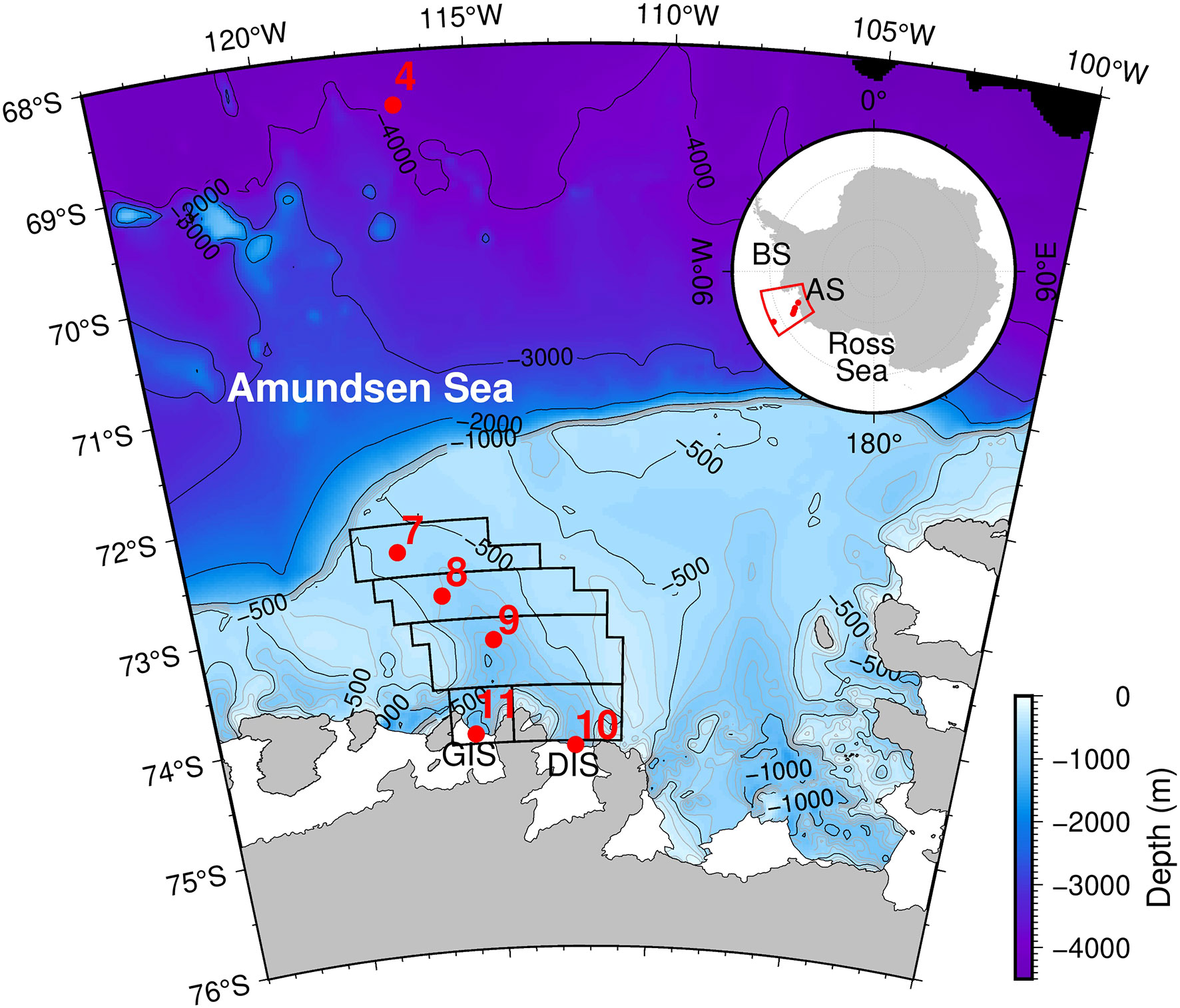
Figure 1 Map depicting sampling locations. The Amundsen Sea (AS) is situated between the Ross and Bellingshausen Seas (BS in the inset). Water samples for the noble gas analysis were collected along the Dotson-Getz Trough (DGT), which links modified circumpolar deep water (mCDW) to the Dotson and Getz Ice Shelves (DIS and GIS). Red circles indicate sampling locations. Black polygons depict the areas considered for calculating the volume of the Dotson-Getz Trough for the melting rate calculation as mentioned in Section 3.5.

The isotopic ratio of He (δ¹⁸He) reported in this study is defined as

$\begin{array}{ll}{\delta }^{3}He(\%)=(\frac{3^{He}{/}^{4}He}{R_A}-1)\times 100& (1)\end{array}$

where R_A is the helium isotopic ratio (³He/⁴He) in the atmosphere (1.384 x 10^-6; Clarke et al., 1976).

The saturation anomaly of each noble gases (ΔC) was calculated from the equation

$\begin{array}{ll}\text{Δ}C(\%)=\left(\frac{C}{C_{eq}}-1\right)\times 100,& (2)\end{array}$

where C_eq is the concentration of each noble gas at equilibrium with the atmosphere (Wood and Caputi, 1966; Weiss, 1971; Weiss and Kyser, 1978; Hamme and Emerson, 2004).

2.2 Optimum multiparameter analysis

Optimum multiparameter analysis assumes that the distribution of tracers is the result of conservative linear mixing of predefined source waters. The analysis requires at least the same number of tracers as that of source waters to find optimal solutions for the fractions of source waters with an overdetermined set of simultaneous equations (Tomczak and Large, 1989). The optimal solutions are determined as the fractions that minimize the residual (R in Eq. 3) between observations and the linear combination of source waters with non-negative constraints on the fractions. We used five noble gases and a He isotope (³He), in addition to potential temperature and salinity, for the tracers of the OMPA.

Two potential source waters at surface layer (AASW and VMW) were added to mCDW, WW, and SMW, often assumed source waters in the CT method (See Section 3.2 for the definitions of the source waters). The system of linear equations of the tracers is represented as

$\begin{array}{ll}\left(\begin{array}{ccccc}{T}_{mCDW}& T_{WW}& T_{AASW}& T_{SMW}& T_{VMW}\\ S_{mCDW}& S_{WW}& S_{AASW}& S_{SMW}& S_{VMW}\\ 3^H{e}_{mCDW}& 3^H{e}_{WW}& 3^H{e}_{AASW}& 3^H{e}_{SMW}& 3^H{e}_{VMW}\\ 4^H{e}_{mCDW}& 4^H{e}_{WW}& 4^H{e}_{AASW}& 4^H{e}_{SMW}& 4^H{e}_{VMW}\\ N{e}_{mCDW}& N{e}_{WW}& N{e}_{AASW}& N{e}_{SMW}& N{e}_{VMW}\\ A{R}_{mCDW}& A{r}_{WW}& A{r}_{AASW}& A{r}_{SMW}& A{r}_{VMW}\\ K{r}_{mCDW}& K{r}_{WW}& K{r}_{AASW}& K{r}_{SMW}& K{r}_{VMW}\\ X{e}_{mCDW}& X{e}_{WW}& X{e}_{AASW}& X{e}_{SMW}& X{e}_{VMW}\\ 1& 1& 1& 1& 1\end{array}\right)\left(\begin{array}{c}{f}_{mCDW}\\ f_{WW}\\ f_{AASW}\\ f_{SMW}\\ f_{VMW}\end{array}\right)=\left(\begin{array}{l}{T}_{obs}\hfill \\ S_{obs}\hfill \\ 3^H{e}_{obs}\hfill \\ 4^H{e}_{obs}\hfill \\ N{e}_{obs}\hfill \\ A{r}_{obs}\hfill \\ K{r}_{obs}\hfill \\ X{e}_{obs}\hfill \\ 1\hfill \end{array}\right)+R,& (3)\end{array}$

where f is the fraction of the source water and the subscript obs stands for the observed values. As tracers have different value ranges, they were normalized with the mean and standard deviation values of each tracer. The tracers were further weighted to account for the different resolving powers of the source waters and reliabilities, according to Beaird et al. (2015) (Table 1). We set the weight of the unity-sum constraint to 100, which is similar to that of the potential temperature. To assess the uncertainty of the NG-OMPA, we performed a Monte Carlo simulation with 10,000 sets of perturbed tracer properties within the uncertainties of the tracers presented in Table S1. The average and standard deviation of 10,000 solutions were chosen as the final solution and error of the NG-OMPA. The SMW and meteoric fractions (SMW plus VMW) calculated using the NG-OMPA method were compared with those obtained from the conventional CT method and the MET from the δ¹⁸ O method. A summary of the CT and δ¹⁸O methods is provided in the Supplementary Material.

TABLE 1

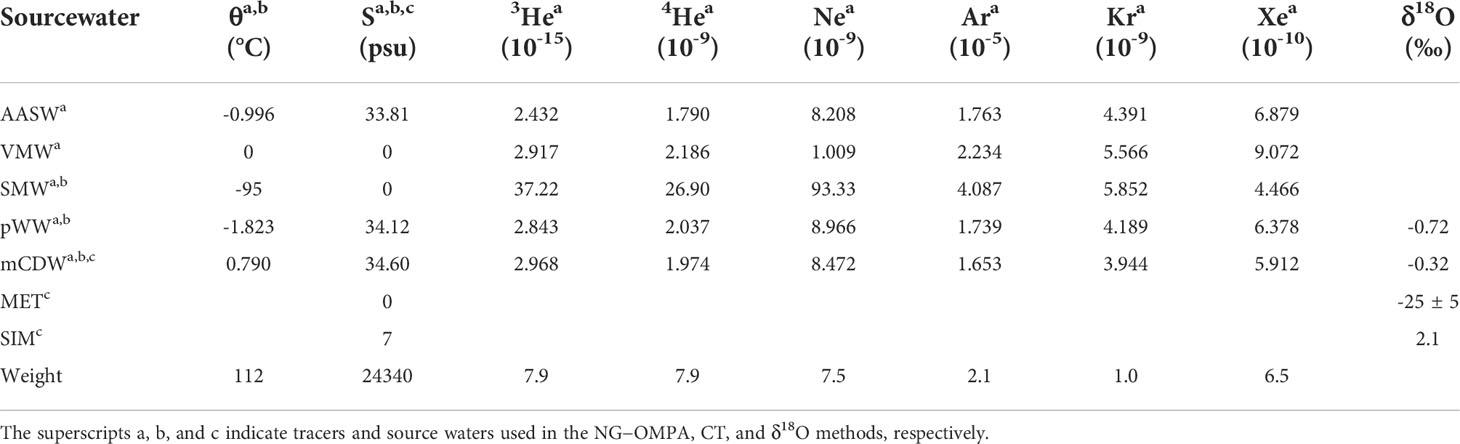
Table 1 Properties of the source waters for water mass analysis. Gas concentration units are mol kg^-1.

3 Results and discussion

3.1 Vertical distributions of the tracers

The vertical profiles of the potential temperature and salinity revealed the major water masses (mCDW, WW, and AASW) in the Amundsen Sea (Figure 2A, B). The warm and saline mCDW (θ ≈ 0.73°C and S ≈ 34.6 psu) occupied the deep layer (>400 m) in the DGT. WW with a relatively low temperature and salinity (θ ≈ -1.8°C and S ≈ 34.1 psu) was observed above the mCDW at depths of <300 m. Higher temperatures and salinities were observed at mid-depths (200 – 400 m) in front of the DIS at Station 10. The increase in temperatures and salinities has been ascribed to active vertical mixing between the mCDW and WW near the DIS (Kim et al., 2016b). AASW, with a higher temperature and lower salinity than the WW, resided in the surface layer. Increased solar radiation and ice melting in the summer contributed to the formation of the AASW.

FIGURE 2

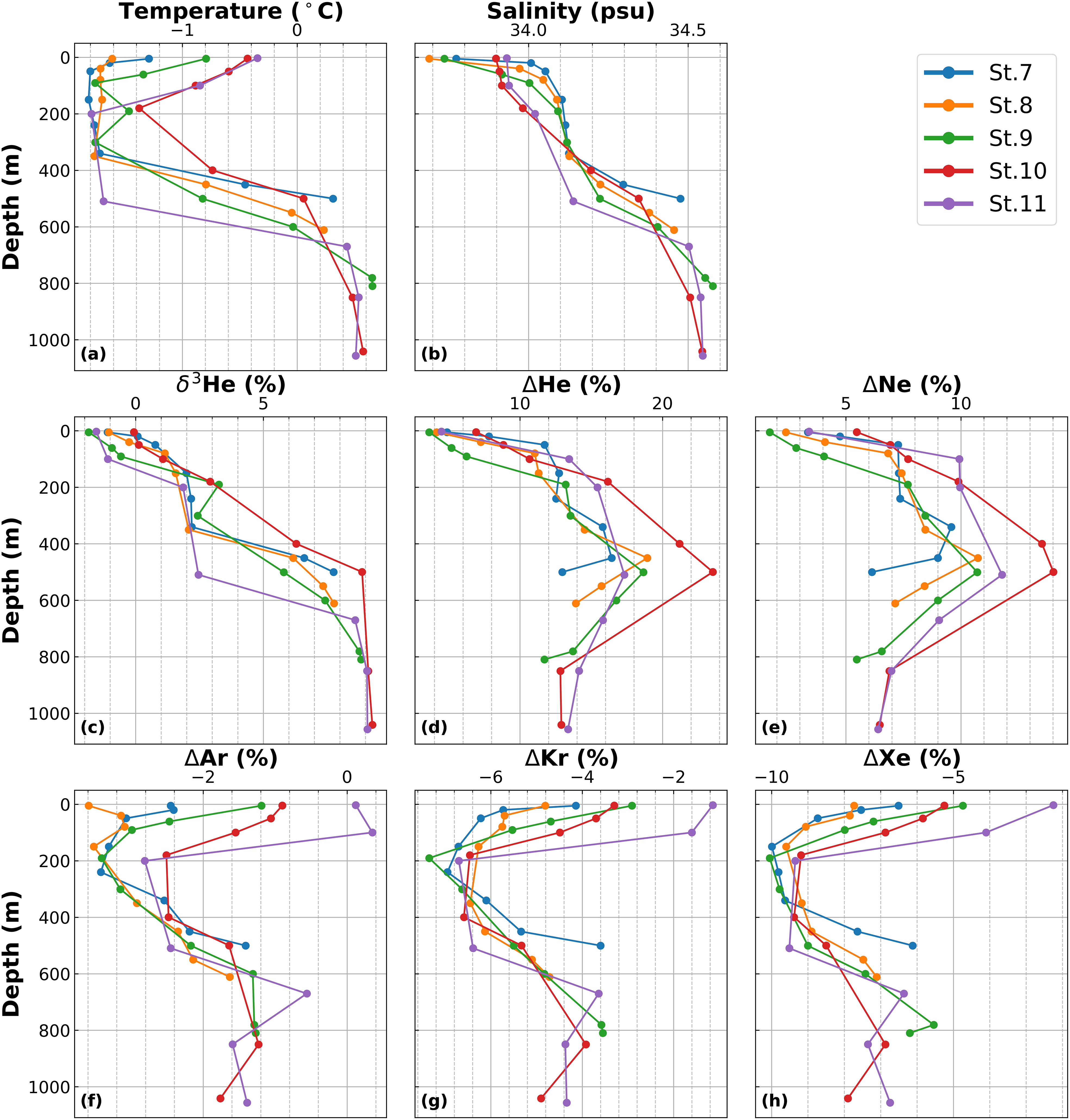
Figure 2 Vertical profiles of the tracers used for the NG-OMPA. (A) Potential temperature, (B) salinity, and (C) isotopic ratio of helium defined as δ³He = [(³He/⁴He) _sample/R_A - 1]× 100,where (³He/⁴He) _sample is the measured ratio of a sample and R_A is the isotopic ratio of the atmosphere. (D−H) Saturation anomalies of the noble gases, defined as (C_sample/C_sat - 1)100, where C_sample and C_sat are the measured and solubility equilibrium concentrations, respectively.

The saturation anomalies of light noble gases (ΔHe and ΔNe) were higher at depths of 400 – 600 m along the DGT than in the upper and deep layers (Figure 2D, E). The maximum ΔNe gradually decreased from 14% in front of the DIS to 9% at Station 7, accompanying an increase in the distance from the DIS. This phenomenon has been attributed to mixing with ambient water as glacial meltwater spreads away from the DIS (Kim et al., 2016b). In the upper layer, the saturation anomalies decreased with an increase in gas exchange with the atmosphere. ΔHe was higher than ΔNe at similar depths (e.g., 24% vs. 14% at Station 10). The elevated He concentration accompanied by a positive δ³He indicates additional input of mantle He from the submarine hydrothermal system. The Pacific sector of the Southern Ocean is known to have a larger mantle He signal because the deep water accumulates hydrothermal helium during meridional overturning circulation, and the Pacific has higher mid-ocean ridge spreading rates (Jenkins, 2020). The highest δ³He values in the mCDW layer were also consistent with the input of hydrothermal helium with high ³He/⁴He ratios (Figure 2C). Crustal He is another source of excess He. Crustal He accumulates in the bedrocks of glaciers by α-decay of U/Th-series radionuclides and has ³He/⁴He ratio markedly lower than the atmosphere (Craig and Scarsi, 1997). Although the crustal He is known to be incorporated into glacial meltwater in the Greenland (Beaird et al., 2015; Huhn et al., 2021), this component should be negligible in the Amundsen Sea given that ³He/⁴He ratios in the Amundsen Sea are explained by the the addition of SMW, which has “air-like” isotopic ratio, to the CDW (Refer to Figure 4 of Kim et al., 2016b). We note that the He (³He and ⁴He) and Ne data were the same as those reported by Kim et al. (2016b).

Although light noble gases showed supersaturation in the DGT, the heavy noble gases (Ar, Kr, and Xe) were undersaturated at all depths (Figure 2F–H). The undersaturation of heavy noble gases is attributed to rapid cooling during water formation (Hamme and Severinghaus, 2007). Because heavy noble gases are more soluble and temperature-sensitive than the light gases, if newly formed water does not remain on the surface long enough for the gases to re-equilibrate with the atmosphere, the heavy gases will remain undersaturated. The lowest saturation anomalies observed at the depths of the WW layer (200 – 500 m) further indicate that sea ice cover obstructs gas exchange (Rutgers van der Loeff et al., 2014) during WW-forming vertical mixing, resulting in intensified undersaturation of the heavy noble gases. In the surface layer above the WW layer, the saturation anomalies increased owing to the temperature increase induced by solar irradiation and enhanced air−sea gas exchange by sea ice melting in summer.

3.2 Source waters for the NG-OMPA

Because both the CT and δ¹⁸O methods use a pair of tracers, they are bound to represent only three source waters, lacking the representation of potential source waters in the upper layer. In Figure 3A, some of the observed values lie outside the triangle created by the mixing lines among the three often-presumed source waters: mCDW, WW (pure WW, pWW), and SMW. The outliers are more clearly visible in the He vs. salinity plot (Figure 3B, and S1 for other noble gases). Most of the samples from depths <200 m plotted close to binary mixing between pWW and AASW. This finding indicates that the addition of AASW as a source water and noble gases as tracers can improve the estimation of SMW near the surface layer. We also considered the VMW, in addition to the usual mCDW, WW, and SMW, as a source water at the surface. VMW may largely represent ventilated meltwater either from upwelled SMW or from laterally transported meltwater at the surface, both of which spend sufficient time (>1 – 2 weeks) to equilibrate with the atmosphere. It is noted that the SIM was not considered as a source water in the NG-OMPA. Although the SIM is considered as a source water in the δ¹⁸O method, its contribution to the Amundsen Sea is negative, indicating the dominance of sea ice formation rather than of sea ice melting (Randall-Goodwin et al., 2015; Bett et al., 2020). Although the constraint of non-negativity when using the NG-OMPA method does not allow for explicit inclusion of the SIM, the effects of sea ice melting in summer and formation in winter were implicitly incorporated into the properties of pWW and AASW, respectively, in the NG-OMPA. The tracer properties of the five source waters are defined in the following subsections and summarized in Table 1.

FIGURE 3

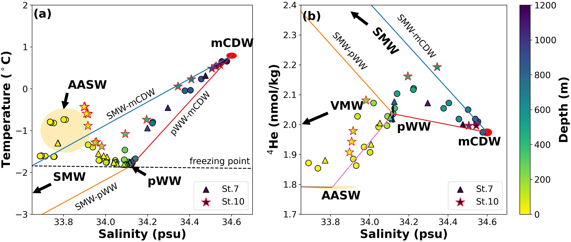
Figure 3 Bivariate plots of (A) potential temperature−salinity and (B) ⁴He−salinity. The circles, triangles, and stars represent samples collected in the DGT. Many samples in the shallow layer (≤200 m) plot above the line of binary mixing between mCDW and SMW in (A). These samples plot along the line of binary mixing between pWW and AASW in (B), suggesting that AASW is necessary as an additional source water for NG-OMPA. The orange and red shades represent the variabilities of AASW and mCDW, respectively.

3.2.1 Antarctic surface water

The AASW, present during spring and summer in the surface layer, has a wide range of temperatures and salinities owing to different degrees of solar insolation and ice melting. We set the temperature and salinity of the AASW to the average of the observed values in the upper 50 m at stations without sea ice (Stations 8 – 10). The concentrations of the noble gases were set to the solubility equilibrium values at the temperature and salinity of the AASW (Wood and Caputi, 1966; Weiss, 1971; Weiss and Kyser, 1978; Hamme and Emerson, 2004). The surface samples plotted close to the mixing line between pWW and AASW (Figure 3B). As the uncertainties in temperature and salinity propagate into the solubility concentrations of gases, the noble gas concentrations in the AASW were perturbed in the range of concentrations defined by the standard deviations in the temperature and salinity of the AASW observed in the Monte Carlo simulation (Table S1).

3.2.2 Ventilated meltwater

VMW potentially represents all freshwater in solubility equilibrium with the atmosphere, including the surface melt of icebergs, ice shelves, and direct precipitation to the ocean. These freshwaters may be produced in the DGT and transported from the upstream such as Pine Island Bay in the Amundsen Sea, and the Bellingshausen Sea (Nakayama et al., 2014; St-Laurent et al., 2019). The VMW also includes ventilated SMW, which has reached the surface after the melting of ice shelves and icebergs at depth and spent some time (>1 – 2 weeks) equilibrating with the atmosphere. We set the temperature and salinity of the VMW to 0°C and 0 psu, respectively. The noble gas concentrations were set to the solubility equilibrium values at the given temperature and salinity.

3.2.3 Modified circumpolar deep water

The temperature and salinity of the mCDW were determined as the intersection between the SMW−mCDW and WW−mCDW mixing lines that enveloped the values observed in 2011 (Jenkins et al., 2018). To account for potential sampling bias, the uncertainties in temperature and salinity were set to include the mCDW properties of previous studies (Randall-Goodwin et al., 2015; Jenkins et al., 2018). The noble gas concentrations were set to the averages of the samples with the highest temperature and salinity found at depths > 800 m at Stations 9–11.

3.2.4 ‘Pure’ winter water

WW, which is replenished every winter by heat loss to the atmosphere and deep mixing, is colder and fresher than the mCDW. Because the observed WW in summer often contains a small fraction of other source waters, we defined ‘pure’ WW (pWW) according to Jenkins et al. (2018). Briefly, the temperature and salinity were set to the point where the extension of the mixing line between the mCDW and the observed WW met the freezing line in the T−S diagram (Figure 3A). The properties of pWW should be determined from each year’s measurements to properly reflect the inter-annual variability of water masses in the Amundsen Sea (Dutrieux et al., 2014; Jenkins et al., 2018). The difference in temperature and salinity properties between the observed WW and pWW indicates that the observed WW was produced by the addition of 0.6% mCDW to pWW. The noble gas concentrations in the pWW were calculated from those in the mCDW and the observed WW, considering the mixed fractions of the water masses. The noble gas concentrations in the observed WW were set to the average values observed at depths of 200 – 350 m at Stations 7 and 8, where sea ice appeared to stabilize the upper water column.

3.2.5 Submarine meltwater

The temperature of the SMW was set to an effective potential temperature of -95°C, which takes account of the heats required for ice to warm to freezing point, for phase change from ice to water, and for mixing with ambient water (Jenkins, 1999). The salinity of SMW was set to 0 psu. The noble gas concentrations were determined as the concentrations in the air bubbles (0.11 cm³ in glacial ice; Martinerie et al., 1992), assuming complete dissolution of the air under high pressure at the depth of basal melting (Schlosser, 1986).

3.3 Distributions of source waters

The deep layer (>500 m) along the DGT appeared to be occupied by >80% mCDW (Figure 4). This is consistent with previous observations indicating persistent inflow of mCDW along the DGT (Wåhlin et al., 2010; Randall-Goodwin et al., 2015; Kim et al., 2016b). The mid-depth layer above the mCDW was occupied by WW. The partially ice-covered areas (near Station 7 with an ice fraction of approximately ~50%) retained large fractions of WW (>70%), even at the surface. In contrast, the surface layer within the Amundsen Sea Polynya (Stations 9 and 10) was largely occupied by AASW (>50%).

FIGURE 4

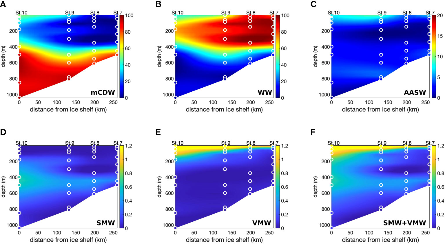
Figure 4 Fractional contributions of different source waters (A–F) for the section along the Dotson-Getz Trough calculated by the NG-OMPA. Fractions at the water sample locations (circles) are superimposed on the interpolated values. Five noble gases, in addition to temperature and salinity, were used as tracers for the analysis. The values shown are the averages of 10,000 results produced by Monte Carlo simulation.

The SMW fractions were most prominent at Station 10 in front of the DIS, with the highest values at depths of 400 – 600 m (>0.6%). These depths are close to the underside of the DIS at ~400 m depth (Gourmelen et al., 2017). The SMW was observed to spread out along the approximately 500 m-deep layer between mCDW and WW. On reaching Station 7, near the continental shelf break, the SMW fraction decreased to 0.2%. This result is in good agreement with previous studies that reported the spreading of SMW beyond the continental shelf break (Randall-Goodwin et al., 2015; Kim et al., 2016b).

Notable fractions of VMW (0.5 – 0.9%), along with the dominant AASW, existed in the surface layer in the DGT. The penetration of VMW was more pronounced at Station 10, with a VMW fraction > 0.4% as deep as 200 m. This higher VMW fraction may be attributed to the direct input of subaerial meltwater from the adjacent DIS, ventilated SMW, and/or the advection of upstream meltwater laden on the westward-flowing coastal currents (Nakayama et al., 2014; St-Laurent et al., 2017). Previous modeling studies have predicted surface meltwater fractions in the range of 0.4 – 1.5% in the DGT ( (Kimura et al., 2017; St-Laurent et al., 2019) consistent with our total SMW and VMW fractions of approximately 1% (Figures 5, 6). The persistently high VMW fractions north of the DIS (Stations 7 and 8) may be ascribed to the clockwise circulation of meltwater around the edges of the DGT (St-Laurent et al., 2017). Alternatively, VMW may result from the melting of icebergs drifting from the east of the trough, which can be an important source of freshwater at the surface (Mazur et al., 2019; Bett et al., 2020). The profiles of the tracers reconstructed from the NG-OMPA predicted fractions of the source waters were comparable to the observed profiles of the tracers (Figures S2 and S3); the profiles of temperature and salinity with higher weightings for optimization were virtually identical to the observed profiles.

FIGURE 5

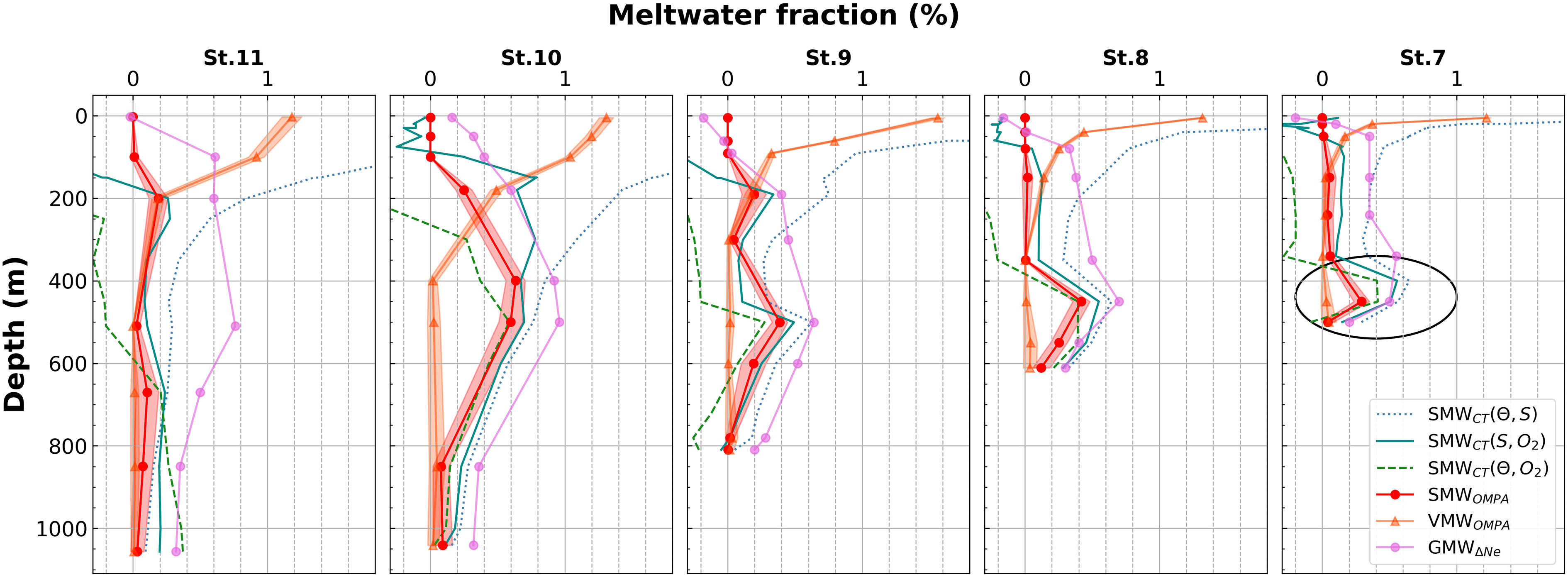
Figure 5 Comparison of SMW fractions calculated by the NG-OMPA and CT methods. Red lines and shaded areas show the averages and the uncertainties of NG-OMPA method. The uncertainties are one standard deviation of 10,000 fractions calculated by Monte Carlo simulation with perturbed values. SMW fractions calculated by the CT method with different pairs of tracers are shown as teal lines. The circle at the bottom of Station 7 highlights a large discrepancy between the SMW fractions estimated by the NG-OMPA and CT methods. Given the lower ΔHe and ΔNe at Station 7 (Figure 2), compared with those at Station 10, it is likely that the SMW fraction at Station 7 is lower than that at Station 10. The fractions of ventilated SMW (VMW) calculated by the NG-OMPA are shown as orange lines. The fractions of glacial meltwater derived from excess Ne are depicted as purple lines.

FIGURE 6

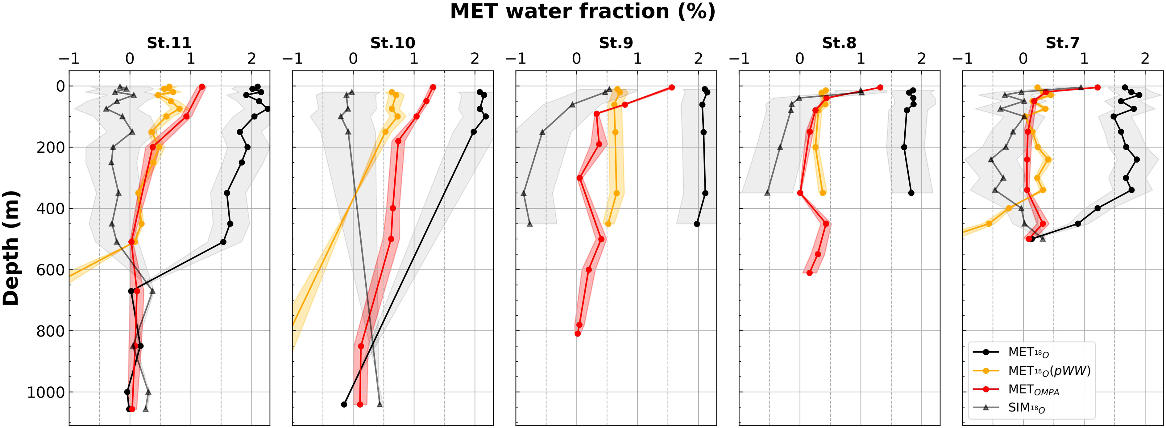
Figure 6 Comparison of MET fractions calculated by the NG-_OMPA (MET_OMPA = SMW + VMW) and δ¹⁸O methods. The MET fractions calculated using the δ¹⁸O method with mCDW as a source water, in addition to SIM and MET, are shown in black. If pWW, instead of mCDW, is considered as a source water, the differences in the fractions calculated by the δ¹⁸O (shown as orange lines) and NG-OMPA methods (shown as red lines) become smaller. SIM_18O are the fraction of sea ice meltwater calculated using δ¹⁸O method. Negative fractions of SIM_18O indicate sea ice formation.

3.4 Improvement on the estimation of submarine glacial meltwater

Both the NG-OMPA and CT methods yielded similar SMW fractions in the mid-depth layer between 400 and 600 m (Figure 5). One notable discrepancy is the gradual decrease in SMW fractions from near the ice shelf to the continental shelf break (0.6% to 0.2%) when employing the NG-OMPA method (SMW_OMPA). This decrease was consistent with the fact that the saturation anomalies of Ne (ΔNe), which are proportional to the meltwater fractions, decreased gradually from the ice shelf to the shelf break (Figure 2E). In contrast, the fractions obtained using the CT method did not vary remarkably, with values ranging from 0.8% to 0.6%, resulting in an overestimation of 0.4% at Station 7. The degrees of deviation from the WW−mCDW mixing line to the SMW property, which is proportional to the meltwater fraction, were not significantly different for the water samples at Stations 7 and 10 (Figure 3A). However, the samples from Station 10 plotted further above the WW−mCDW mixing line in the He salinity plot than did those from Station 7 (Figure 3B), suggesting higher SMW fractions. In the upper layer, the three SMW fractions estimated using CT method with different pairs of tracers deviated from one other because there was no source water defined to account for atmospheric interaction and additional freshwater sources (Jenkins and Jacobs, 2008). The overall similarity between the fractions obtained by the salinity−O₂ pair and the SMW_OMPA fractions also supports the plausibility of the NG-OMPA method. Jenkins and Jacobs (2008) argued that the counteracting effects of freshening of salinity and air–sea equilibrium of O₂, respectively, fortuitously compensate for each other and produce the most reliable SMW estimates among the three tracer pairs in the surface layer.

The SMW_OMPA fractions appeared to be smaller than those estimated using the He and Ne concentrations alone (Kim et al., 2016b). The authors attributed the He and Ne excess over the concentrations at a background site located 400 km north of the continental shelf break of the Amundsen Sea to glacial melting. Intrinsically, the SMW fractions by Kim et al. (2016b) represent meltwater added within the DGT as well as those added during the transit of the water mass from off the continental shelf to the trough. If the water mass overwintered in the trough, the fractions would also include meltwater from the previous year, incorporated through WW-forming vertical mixing. In this respect, a slightly higher meltwater fraction estimated from excess Ne over the background concentrations (GMW_ΔNe) than SMW_OMPA (Figure 5) is not surprising because the latter represents meltwater addition after the most recent WW formation. The largest discrepancy between GMW_ΔNe and SMW_OMPA (0.7% vs. approximately 0% at 500 m at Station 11) was found in front of the GIS (Figure 5). This finding indicates that the majority of GMW_ΔNe was added to the layer via vertical mixing in winter, while meltwater addition after the formation of WW was negligible near the GIS. The apparently lower basal melting rate may have also resulted from weaker intrusion of mCDW into the cavity of the GIS compared with that in the DIS. While previous hydrographic observations have indicated that strong inflow and outflow existed on the eastern and western sides of the DIS front, a similar along-shelf hydrographic variation indicating strong flows was not found in front of the GIS (Randall-Goodwin et al., 2015; Kim et al., 2016b). The deviation of GMW_ΔNe from SMW_OMPA became most pronounced in the layer occupied by WW (100 – 400 m), where the fraction of pWW was high (Figure 4). The conservation of excess Ne in the WW layer corroborates the suggestion that gas exchange at the time of WW formation is restricted by sea ice cover (Rutgers van der Loeff et al., 2014).

3.5 Calculation of basal melting rate from the SMW fractions

To convert the SMW fractions to the amount of meltwater, we calculated the mean fractions at each station for the upper and deep layers of the water column by integrating the vertical profile of the SMW fractions at each site with the corresponding depth intervals. The boundary between the two layers was set to 300 m according to St-Laurent et al. (2017). The researchers regarded the upper layer as subject to deep convection that replenished it with nutrients and dissolved iron in winter. Furthermore, they argued that iron, which supports high primary production in summer, is mainly supplied to the upper layer by buoyancy-driven overturning circulation, the so-called “meltwater pump” (St-Laurent et al., 2017; St-Laurent et al., 2019). The mean fractions of the upper and deep layers at each sampling site were assumed to be representative of the water column adjacent to the site. The eastern and western boundaries of the water columns roughly followed the ridges flanking the DGT (see the polygons in Figure 1). The mean fractions were multiplied by the volume of the layers and the resultant SMW amounts were 8.9 km³ and 22.3 km³ for the upper and deep layers, respectively (Table 2).

TABLE 2

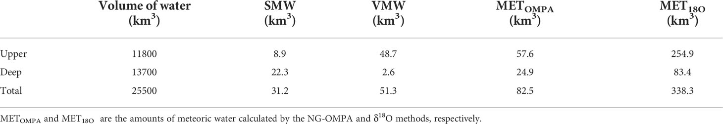
Table 2 Meltwater in the upper (<300 m) and deep layers of the Dotson-Getz Trough. SMW and VMW stand for submarine meltwater and ventilated meltwater, respectively.

It is likely that the SMW in the deep layer is produced within the DGT because the Bear Ridge, located on the eastern side of the DGT, rises to <300 m below the sea surface, prohibiting the direct input of upstream glacial meltwater to the deep layer (St-Laurent et al., 2019; Bett et al., 2020). However, it is difficult to specify the origin of the SMW in the upper layer at a depth of approximately 200 m (Figure 4) because westward-flowing coastal currents may carry upstream glacial meltwater to the DGT (Nakayama et al., 2014). We speculate that the coastal currents mostly carry VMW rather than SMW, based on the observations showing that the coastal currents were mostly confined to the surface layer <100 m (Kim et al., 2016a). Additional support for this speculation comes from the fact that upstream glacial meltwater, mainly from the Pine Island Ice Shelf, travels for several months with a mean westward velocity of 0.03 m s^-1 (Nakayama et al., 2014) to reach the DGT, providing enough time to equilibrate with the atmosphere.

To deduce the basal melting rates of the ice shelves in the DGT, we assumed that the SMW fraction represents meltwater accumulated after the formation of the WW because pWW is included as a source water in the NG-OMPA. Owing to the lack of direct observation, it is difficult to specify when pWW forms. We used a time series of climatological sea ice concentrations (Figure S2) to infer probable months in which the properties of the pWW were set. We postulate that the rapid increase in the sea ice concentration in March and April and resultant brine rejection promote pWW formation, the properties of which do not change markedly when sea ice concentrations are close to the maximum (≥90% from June to August). Consequently, the SMW fractions observed in early January 2011 reflect the amount of SMW introduced over the past 4 – 7 months, depending on the timing of pWW formation. The basal melting rate was estimated to be in the range of 53 – 94 Gt yr^-1 by combining an SMW amount of 31.2 km³ during a duration of 4 – 7 months. If only the amount of SMW in the deep layer is taken into consideration, the melting rate becomes 38 – 67 Gt yr^-1. However, we favor the estimates that include SMW amounts from both the upper and deep layers because the depths of approximately 200 m, where the SMW fraction in the upper layer is high, are similar to the depths with a strong outflow of melt-laden overturned water from the DIS (Randall-Goodwin et al., 2015; Kim et al., 2016b). This suggests that 29% (8.9 km³ out of 31.2 km³) of the SMW produced in the DGT is upwelled to the upper layer. This upwelled SMW is eventually brought to the surface layer by deep convection in winter and replenishes the surface layer with iron, which is in turn available for primary production in the subsequent summer. The estimates of the basal melting rate were mostly ascribed to the DIS because the SMW amount of 1.9 km³ in the water column adjacent to the GIS (Figure 1) was only 6% of the total amount of SMW.

Although our estimates have a relatively large range owing to the uncertain timing of pWW formation, the melting rates are in the range of previous estimates for the DIS. For example, Jenkins et al. (2018) demonstrated a large temporal variation in the melting rate in the range of 20 – 90 Gt yr^-1 from 16 years of CTD observations in front of the DIS. They estimated a melting rate of 55 ± 15 Gt yr^-1 in 2011. Similarly, Rignot et al. (2013) estimated a melting rate of 45 ± 4 Gt yr^-1 using 2003 – 2008 satellite data. Because melts near the surface are subject to gas exchange and classified as VMW in the NG-OMPA, the basal melting rate calculated from SMW alone should be considered a lower bound.

3.6 Comparison of meteoric water fractions from the NG-_OMPA and δ¹⁸O methods

Both the SMW and VMW from the NG-OMPA constitute meteoric water, i.e., freshwater originated from the atmosphere, either as falling snow or melts of glacial ice. While SMW dominated the sum of the SMW and VMW fractions (MET_OMPA) in the deep layer, VMW became the major component of MET_OMPA at the depths <200 m (Figures 5, 6 and Table 2). The MET_OMPA fractions did not exceed 0.6%, except in the upper layer where the values were as high as 1.5%. It is intriguing that the MET_OMPA fractions were much less than the meteoric water fraction estimated by the δ¹⁸O (MET_18O; Meredith et al., 2008; Randall-Goodwin et al., 2015). The latter fractions were obtained by assuming the often-adopted three source waters: MET, SIM, and mCDW (refer to Supplementary Material for the method). Most of the fractions of MET_18O fell within a narrow range of 1.5 – 2% from the surface to >400 m depths (Figure 6).

We speculate that the large discrepancy between MET_OMPA and MET_18O results from the fact that the δ¹⁸O method calculates meteoric fractions accumulated relative to the mCDW. In contrast, the NG-OMPA, which includes pWW as a source water, estimates the meteoric water accumulated since the previous pWW formation. This speculation seems plausible, given the fact that if mCDW is replaced with pWW, the δ¹⁸O method gives meteoric water fractions similar to MET_OMPA (MET_18O (pWW) in Figure 6) This also suggests that the inventory of meteoric water in the DGT (MET_18O) is much larger than the amount of meteoric water accumulated since the previous pWW formation (MET_OMPA). The four times larger inventory (Table 2) may be ascribed to the combined effects of high meteoric water content at the surface and periodic delivery of the surface water to the deep layer by deep convection in winter. The negative SIM fraction from the δ^18O method (SIM_18O in Figure 6) implies that brine produced by sea ice formation is delivered to the deep layer in winter. Westward-flowing coastal currents seem to play an important role in keeping the surface layer rich in meteoric water (1 – 2%) by carrying upstream meltwater. The meltwater laden on coastal currents flows along the ice shelves year-round, and part of it spreads along the edges of the DGT, forming a clockwise circulation (St-Laurent et al., 2017). Assuming a volume transport of 4 – 5 Sv for the coastal current (St-Laurent et al., 2019) and a volume of 1.18 × 10⁴ km³ for the seawater in the upper layer (Table 2), the upper layer of the DGT is replaced every month with upstream water. Although it is often implicitly assumed that MET is proportional to the melting rate of adjacent ice shelves, it appears that MET_18O represents accumulation relative to mCDW, integrating meltwaters from a larger space and time compared with SMW estimated using CT or NG–OMPA methods.

4 Concluding remarks

In this study, noble gases were used as additional tracers in the OMPA method to separate ventilated and submarine meltwaters in the Dotson-Getz Trough in the Amundsen Sea.The increased number of tracers provided better constraints on the distribution of glacial meltwater on the surface. We demonstrated that noble gases are an invaluable set of tools that can be used for verifying and correcting the meltwater distributions depicted using the CT method. Clear identification of SMW and VMW allowed us to provide a reasonable basal melting rate of 53 – 94 Gt yr^-1 for ice shelves in the DGT. Information on the timing of winter water formation is important for reducing the uncertainty regarding the melting rate. This information may be obtained from overwinter time-series observations of the physical and chemical tracers used in the NG-OMPA.

The meteoric fractions obtained from the NG-OMPA, assumed to be the sum of SMW and VMW, were four-fold lower than those obtained using the δ¹⁸O method with mCDW as one of the source waters. While the meteoric fractions determined using NG-OMPA represent locally produced fractions since the previous WW formation, the fraction from the δ¹⁸O method appeared to represent the amount of meteoric water accumulated over multiple years, which was likely strongly influenced by upstream meltwater. To better understand the distribution of meteoric water and its potential impact on bottom water formation in downstream regions, it is necessary to collect information on meltwater transport to and from the upper layer, under the strong influence of westward-flowing coastal currents, and the propagation of surface meltwater to the deep layer by vertical mixing in winter. Thus, separation of VMW from SMW using NG-OMPA and comparison with MET from the δ¹⁸Omethod is an important tool for distinguishing upstream meltwater from locally produced waters.

Data availability statement

The datasets for this study can be found in the Korea Polar Data Center (http://kpdc.kopri.re.kr) with the data ID of KOPRI-KPDC-00001633.

Author contributions

DH and TR contributed to conception and design of the study. DS and DH were responsible for data analysis and writing the manuscript. SL conceived the project and led the fieldwork. T-WK, KP, JP, YK, MK and TL contributed to discussion and the data acquisition during cruises. All authors contributed to manuscript revision, read, and approved the submitted version.

Funding

This work was supported by grant from Korea Polar Research Institute PE22110 and PE21140 funded by the Ministry of Oceans and Fisheries. DS and DH were partially supported by the Basic Science Research Program through the National Research Foundation of Korea (NRF) funded by the Ministry of Science and ICT (NRF-2020R1A2C1009440).

Acknowledgments

We thank the captain and all the crew members of Araon for the help on board. The constructive comments from the reviewers and editor have greatly improved the manuscript.

Conflict of interest

The authors declare that the research was conducted in the absence of any commercial or financial relationships that could be construed as a potential conflict of interest.

Publisher’s note

All claims expressed in this article are solely those of the authors and do not necessarily represent those of their affiliated organizations, or those of the publisher, the editors and the reviewers. Any product that may be evaluated in this article, or claim that may be made by its manufacturer, is not guaranteed or endorsed by the publisher.

Supplementary material

The Supplementary Material for this article can be found online at: https://www.frontiersin.org/articles/10.3389/fmars.2022.951471/full#supplementary-material

References

Arrigo K. R., van Dijken G. L., Strong A. L. (2015). Environmental controls of marine productivity hot spots around Antarctica. J. Geophys. Res. 120, 5545–5565. doi: 10.1002/2015JC010888

CrossRef Full Text | Google Scholar

Beaird N. L., Straneo F., Jenkins W. (2015). Spreading of Greenland meltwaters in the ocean revealed by noble gases. Geophys. Res. Lett. 42, 7705–7713. doi: 10.1002/2015GL065003

CrossRef Full Text | Google Scholar

Beaird N. L., Straneo F., Jenkins W. (2018). Export of strongly diluted Greenland meltwater from a major glacial fjord. Geophys. Res. Lett. 45, 4163–4170. doi: 10.1029/2018GL077000

CrossRef Full Text | Google Scholar

Bett D. T., Holland P. R., Naveira Garabato A. C., Jenkins A., Dutrieux P., Kimura S., et al. (2020). The impact of the amundsen Sea freshwater balance on ocean melting of the West Antarctic ice sheet. J. Geophys. Res. 125, 1–18. doi: 10.1029/2020JC016305

CrossRef Full Text | Google Scholar

Biddle L. C., Heywood K. J., Kaiser J., Jenkins A. (2017). Glacial meltwater identification in the amundsen Sea. J. Phys. Oceanogr. JPO–D–16–0221.1–22, 933–954. doi: 10.1175/JPO-D-16-0221.1

CrossRef Full Text | Google Scholar

Biddle L. C., Loose B., Heywood K. J. (2019). Upper ocean distribution of glacial meltwater in the amundsen Sea, Antarctica. J. Geophys. Res. 124, 6854–6870. doi: 10.1029/2019JC015133

CrossRef Full Text | Google Scholar

Cape M. R., Straneo F., Beaird N., Bundy R. M., Charette M. A. (2019). Nutrient release to oceans from buoyancy-driven upwelling at Greenland tidewater glaciers. Nat. Geosci. 12, 1–9. doi: 10.1038/s41561-018-0268-4

CrossRef Full Text | Google Scholar

Clarke W. B., Jenkins W. J., Top Z. (1976). Determination of tritium by mass spectrometric measurement of 3He. Int. J. Appl. Radiat. Isotopes. 27, 515–522. doi: 10.1016/0020-708X(76)90082-X

CrossRef Full Text | Google Scholar

Craig H., Scarsi P. (1997). Helium isotope stratigraphy in the gisp2 ice core. EOS. Trans. Am. Geophys. Union. 78, F7.

Google Scholar

Depoorter M. A., Bamber J. L., Griggs J. A., Lenaerts J. T. M., Ligtenberg S. R. M., van den Broeke M. R., et al. (2013). Calving fluxes and basal melt rates of antarctic ice shelves. Nature. 502, 89–92. doi: 10.1038/nature12567

PubMed Abstract | CrossRef Full Text | Google Scholar

Dutrieux P., De Rydt J., Jenkins A., Holland P. R., Ha H. K., Lee S. H., et al. (2014). Strong sensitivity of pine island ice-shelf melting to climatic variability. Science 343, 174–178. doi: 10.1126/science.1244341

PubMed Abstract | CrossRef Full Text | Google Scholar

Gourmelen N., Goldberg D. N., Snow K., Henley S. F., Bingham R. G., Kimura S., et al. (2017). Channelized melting drives thinning under a rapidly melting antarctic ice shelf. Geophys. Res. Lett. 44, 9796–9804. doi: 10.1002/2017GL074929

CrossRef Full Text | Google Scholar

Hamme R. C., Emerson S. R. (2004). The solubility of neon, nitrogen and argon in distilled water and seawater. Deep-Sea. Res. I. 51, 1517–1528. doi: 10.1016/j.dsr.2004.06.009

CrossRef Full Text | Google Scholar

Hamme R., Severinghaus J. P. (2007). Trace gas disequilibria during deep-water formation. Deep-Sea. Res. Part I. 54, 939–950. doi: 10.1016/j.dsr.2007.03.008

CrossRef Full Text | Google Scholar

Huhn O., Rhein M., Kanzow T., Schaffer J., Sültenfuß J. (2021). Submarine meltwater from nioghalvfjerdsbræ(79 north glacier), northeast greenland. J. Geophys. Res.: Oceans. 126, e2021JC017224. doi: 10.1029/2021JC017224

CrossRef Full Text | Google Scholar

Jacobs S. S., Helmer H. H., Doake C. S. M., Jenkins A., Frolich R. M. (1992). Melting of ice shelves and the mass balance of Antarctica. J Glaciology 38, 375–387. doi: 10.1017/S0022143000002252

CrossRef Full Text | Google Scholar

Jenkins A. (1999). The impact of melting ice on ocean waters. J. Phys. Oceanogr. 29, 2370–2381. doi: 10.1175/1520-0485(1999)029<2370:TIOMIO>2.0.CO;2

CrossRef Full Text | Google Scholar

Jenkins W. J. (2020). Using excess ³He to estimate southern ocean upwelling time scales. Geophys. Res. Lett. 47, e2020GL087266. doi: 10.1029/2020GL087266

CrossRef Full Text | Google Scholar

Jenkins A., Jacobs S. (2008). Circulation and melting beneath George VI ice shelf, Antarctica. J. Of. Geophys. Research-Oceans. 113, C04013. doi: 10.1029/2007JC004449

CrossRef Full Text | Google Scholar

Jenkins A., Shoosmith D., Dutrieux P., Jacobs S., Kim T. W., Lee S. H., et al. (2018). West Antarctic Ice sheet retreat in the amundsen Sea driven by decadal oceanic variability. Nat. Geosci. 11, 733–738. doi: 10.1038/s41561-018-0207-4

CrossRef Full Text | Google Scholar

Kim I., Hahm D., Rhee T. S., Kim T. W., Kim C.-S., Lee S. (2016b). The distribution of glacial meltwater in the amundsen Sea, Antarctica, revealed by dissolved helium and neon. J. Geophys. Res. 121, 1654–1666. doi: 10.1002/2015JC011211

CrossRef Full Text | Google Scholar

Kim C.-S., Kim T.-W., Cho K.-H., Ha H. K., Lee S., Kim H.-C., et al. (2016a). Variability of the Antarctic coastal current in the amundsen Sea. Estuarine. Coast. Shelf. Sci. 181, 123–133. doi: 10.1016/j.ecss.2016.08.004

CrossRef Full Text | Google Scholar

Kimura S., Jenkins A., Regan H., Holland P. R., Assmann K. M., Whitt D. B., et al. (2017). Oceanographic controls on the variability of ice-shelf basal melting and circulation of glacial meltwater in the amundsen Sea embayment, Antarctica. J. Geophys. Res.: Oceans. 122, 10131–10155. doi: 10.1002/2017JC012926

CrossRef Full Text | Google Scholar

Loose B., Jenkins W. J. (2014). The five stable noble gases are sensitive unambiguous tracers of glacial meltwater. Geophys. Res. Lett. 41, 2835–2841. doi: 10.1002/2013GL058804

CrossRef Full Text | Google Scholar

Martinerie P., Raynaud D., Etheridge D. M., Barnola J.-M., Mazaudier D. (1992). Physical and climatic parameters which influence the air content in polar ice. Earth Planet. Sci. Lett. 112, 1–13. doi: 10.1016/0012-821X(92)90002-D

CrossRef Full Text | Google Scholar

Mazur A. K., Wåhlin A. K., Kalén O. (2019). The life cycle of small- to medium-sized icebergs in the amundsen Sea embaymen. Polar. Res. 38, 1–17. doi: 10.33265/polar.v38.3313

CrossRef Full Text | Google Scholar

Meredith M. P., Brandon M. A., Wallace M. I., Clarke A., Leng M. J., Renfrew I. A., et al. (2008). Variability in the freshwater balance of northern Marguerite bay, Antarctic peninsula: Results from δ18O. Deep-Sea. Res. Part II-Topical. Stud. In. Oceanogr. 55, 309–322. doi: 10.1016/j.dsr2.2007.11.005

CrossRef Full Text | Google Scholar

Meredith M. P., Venables H. J., Clarke A., Ducklow H. W., Erickson M., Leng M. J., et al. (2013). The freshwater system West of the Antarctic peninsula: Spatial and temporal changes. J. Climate. 26, 1669–1684. doi: 10.1175/JCLI-D-12-00246.1

CrossRef Full Text | Google Scholar

Nakayama Y., Menemenlis D., Schodlok M., Rignot E. (2017). Amundsen and bellingshausen seas simulation with optimized ocean, sea ice, and thermodynamic ice shelf model parameters. J. Geophys. Res. 122, 6180–6195. doi: 10.1002/2016JC012538

CrossRef Full Text | Google Scholar

Nakayama Y., Timmermann R., Rodehacke C. B., Schroder M., Hellmer H. H. (2014). Modeling the spreading of glacial meltwater from the amundsen and bellingshausen seas. Geophys. Res. Lett. 41, 7942–7949. doi: 10.1002/2014GL061600

CrossRef Full Text | Google Scholar

Östlund H. G., Hut G. (1984). Arctic Ocean water mass balance from isotope data. J. Of. Geophys. Research-Oceans. 89, 6373–6310. doi: 10.1029/JC089iC04p06373

CrossRef Full Text | Google Scholar

Randall-Goodwin E., Meredith M. P., Jenkins A., Yager P. L., Sherrell R. M., Abrahamsen E. P., et al. (2015). Freshwater distributions and water mass structure in the amundsen Sea polynya region, Antarctica. Elementa.: Sci. Anthropocene. 3, 000065–000022. doi: 10.12952/journal.elementa.000065

CrossRef Full Text | Google Scholar

Rignot E., Jacobs S., Mouginot J., Scheuchl B. (2013). Ice-shelf melting around Antarctica. Science. 341, 266–270. doi: 10.1126/science.1235798

PubMed Abstract | CrossRef Full Text | Google Scholar

Rutgers van der Loeff M. M., Cassar N., Nicolaus M., Rabe B., Stimac I. (2014). The influence of sea ice cover on air-sea gas exchange estimated with radon-222 profiles. J. Geophys. Res. 119, 2735–2751. doi: 10.1002/2013JC009321

CrossRef Full Text | Google Scholar

Schlosser P. (1986). Helium: a new tracer in Antarctic oceanography. Nature 321, 233–235. doi: 10.1038/321233a0

CrossRef Full Text | Google Scholar

Stanley R. H. R., Baschek B., Lott D. E., Jenkins W. J. (2009). A new automated method for measuring noble gases and their isotopic ratios in water samples. Geochem. Geophys. Geosyst. 10, 1–18. doi: 10.1029/2009GC002429

CrossRef Full Text | Google Scholar

St-Laurent P., Yager P. L., Sherrell R. M., Oliver H., Dinniman M. S., Stammerjohn S. E. (2019). Modeling the seasonal cycle of iron and carbon fluxes in the amundsen Sea polynya, Antarctica. J. Geophys. Res.: Oceans. 124, 1544–1565. doi: 10.1029/2018JC014773

PubMed Abstract | CrossRef Full Text | Google Scholar

St-Laurent P., Yager P. L., Sherrell R. M., Stammerjohn S. E., Dinniman M. S. (2017). Pathways and supply of dissolved iron in the amundsen Sea (Antarctica). J. Geophys. Res. 122, 7135–7162. doi: 10.1002/2017JC013162

CrossRef Full Text | Google Scholar

Tomczak M., Large D. G. B. (1989). Optimum multiparameter analysis of mixing in the thermocline of the eastern Indian ocean. J. Geophys. Res. 94, 16141–16149. doi: 10.1029/JC094iC11p16141

CrossRef Full Text | Google Scholar

Wåhlin A., Bjork G., Nohr C. (2010). Inflow of warm circumpolar deep water in the central amundsen shelf. J. Phys. Oceanogr. 1427–1434. doi: 10.1175/2010JPO4431.1

CrossRef Full Text | Google Scholar

Weiss R. F. (1971). Solubility of helium and neon in water and seawater. J. Chem. Eng. Data. 16, 235–241. doi: 10.1021/je60049a019

CrossRef Full Text | Google Scholar

Weiss R. F., Kyser T. K. (1978). Solubility of krypton in water and sea water. J. Chem. Eng. Data. 23, 69–72. doi: 10.1021/je60076a014

CrossRef Full Text | Google Scholar

Wood D., Caputi R. (1966). Solubilities of kr and xe in fresh and sea water. Tech. Rep, 1–12. doi: 10.21236/AD0631557

CrossRef Full Text | Google Scholar