Fragility of marine photosynthesis

1 Introduction

Historically, the study of ocean primary production relied on laboratory and field measurements coupled with mathematical models representing photosynthetic processes (Platt and Sathyendranath, 1991; Regaudie-de Gioux et al., 2014), with the goal of capturing the spatial and temporal variability in its magnitude, with increasing use of satellite ocean-colour data in recent decades to capture basin- and global-scale variability (Platt and Sathyendranath, 1988; Longhurst et al., 1995; Sathyedranath et al., 1995; Kulk et al., 2021). These models used radiative transfer and light transmission models to capture the spectrally- and angularly-resolved light field in the ocean, coupled with physiological models of photosynthetic response of phytoplankton to available light.

Another long-standing interest in the oceanographic community has been the role of ocean dynamics in controlling the supply of nutrients into the surface layer of the ocean, and the mixing in the layer, thereby controlling phytoplankton growth and formation of blooms (Sverdrup, 1953; Platt et al., 1991; Sathyendranath et al., 2015; Kovač et al., 2021). There has also been considerable investment of effort in embedding primary production models into large-scale simulation models of marine ecosystems, which in turn are embedded in general circulation models of the ocean (Laufkötter et al., 2015).

In recent years, stability and resilience of primary production have emerged as novel themes in the study of the pelagic ecosystem using analytical models (Kovač et al., 2020). At their core both terms attempt to quantify how sustainable primary production is: a topic of paramount interest due to climate change. Unfortunately, easily measurable and practically quantifiable definitions of both have proven to be rather elusive thus far in case of primary production. While stability, fragility, resilience and tipping points are of general interest in today’s context of a changing climate, phytoplankton primary production is of particular interest: it is, arguably, one of the oldest productive systems on Earth; and though it is known to have undergone long-term changes in regional magnitude over geological time scales, it is not known to have collapsed at any time, to make room for another type of productive system in the pelagic ocean. Efforts to forecast likely changes in primary production over the next century using simulation models have yielded results with large uncertainties (Frölicher et al., 2016; Kwiatkowski et al., 2020), which have been attributed, among other factors, to “incomplete understanding of fundamental processes”. Recent studies of time series of satellite data to extract trends in primary production admittedly suffer from the short length of the time series (Watson and Rouusseaux, 2019; Kulk et al., 2021).

Here we follow an alternative approach, combining marine primary-production models with the rich literature in economics on production theory (Acemoglu, 2009; Perman et al., 2011; Richmond et al., 2013). The two disciplines have not communicated well up to now, and the cross-disciplinary flux of ideas has been virtually non-existent, testifying to the chasm between the two fields, in contrast to other ecological fields where the transfer of knowledge did occur, for example, in fisheries (Clark and Munro, 1975; Munro, 1992).

Of major concern in the context of climate change is the response of primary production to changing surface ocean stratification and consequently mixed-layer depth, which exert a strong control on both phytoplankton blooms and primary production (Da et al., 2021). In Climate Model Intercomparison Project 6 (CMIP6), the surface warming is expected to increase stratification, contributing to shallower mixed layer, a reduction in the supply of nitrogen into the surface layer and a decrease in the ventilation of sub-surface oxygen (Kwiatkowski et al., 2020). For oceanic primary production, variability in the mixed-layer depth presents a strong disturbance, controlling the average light levels in the mixed-layer as well as the supply of nutrients into the layer (Platt et al., 2003b). Mixed-layer shallowing favours phytoplankton growth, as it increases the average light conditions in the mixed layer, whereas mixed-layer deepening decreases it. However, there is an asymmetry in the response of mixed layer production to deepening, in contrast to shallowing. This asymmetry is caused by the exponential light attenuation with depth and the response of production to light, both being nonlinear. In relative terms, shallowing can cause a greater increase in mixed-layer production, than the reduction caused by a mixed-layer deepening of the same magnitude. This asymmetry calls for a re-examination of the notions of stability and resilience in aquatic primary production.

2 Theory

2.1 Photosynthesis irradiance function

Let the rate of carbon assimilation by phytoplankton per unit biomass P^B be given by a photosynthesis irradiance function p^B of the form:

$\begin{array}{ll}{P}^B=p^B(I),& (1)\end{array}$

where irradiance is given as I (Figure 1). In the literature there are numerous examples of photosynthesis irradiance functions (Platt and Jassby, 1976; Jones et al., 2014; Kovač et al., 2017) and the exact mathematical expression for the dependence of production on light varies amongst these functions. However, all exhibit a linear response to light at low irradiance:

$\begin{array}{ll}\underset{I\to 0}{\lim }{p}^B(I)={\alpha }^{B}I& (2)\end{array}$

FIGURE 1

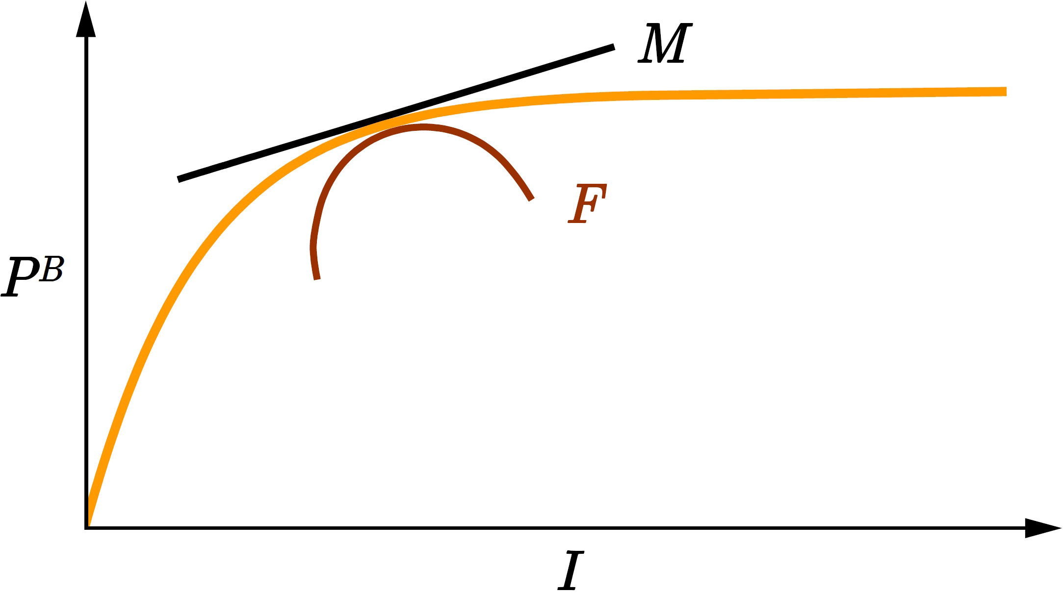
Figure 1 Graphical representation of marginal production M (first derivative, black) and fragility F (second derivative, red) for the photosynthesis irradiance function (orange curve), where production per unit biomass P^B is given asa function of irradiance I.

and a decline in the rate of response with increasing irradiance, which leads to production saturation at high irradiance:

$\begin{array}{ll}\underset{I\to \infty }{\lim }{p}^B(I)=P_m^B& (3)\end{array}$

where α^B is the initial slope and $P_m^B$ is the assimilation number, which setts the rate of carbon assimilation per unit biomass at saturation (Platt and Jassby, 1976; Jassby and Platt, 1976). Mathematically, we say the photosynthesis irradiance function is curved with respect to light (Jones et al., 2014). We should stress that here we do not consider photoinhibition, a phenomenon in which production declines at sufficiently high irradiance (Platt et al., 1980).

The observed decline in the rate of response has consequences for oceanic primary production as it eventually sets an upper limit on how productive the ocean can be. A more subtle consequence of the curvature is manifested in the dynamical response of primary production to perturbations in the light field. In the ocean these perturbations arise naturally over a wide range of temporal and spatial scales. To precisely quantify the effect of irradiance variability on primary production we introduce to the oceanographic literature the notions of marginal production and fragility, inspired by the economic concepts from Taleb (2012). In economics, marginal production quantifies the change in output due to a unit change in input, whereas fragility is a more subtle concept. As investigated by Taleb (2012), fragility and closely related antifragiltiy, arise due to nonlinearities in the response of an output to a change in input. These nonlinear responses may make the system decrease/increase output under stochastic variability of the input, in which case we would say the system is fragile/antifragile. To be mathematically precise and to avoid ambiguity in applying these concepts in the oceanographic literature, we proceed as follows.

First, we define marginal production M:

$\begin{array}{ll}M=\frac{d{p}^B(I)}{dI}& (4)\end{array}$

As is well known, increasing irradiance leads to increasing production, therefore marginal production is positive (Figure 1):

$\begin{array}{ll}M>0& (5)\end{array}$

Marginal production itself is a function of irradiance M=M(I) . To describe how M behaves as a function of I we define fragility as:

$\begin{array}{ll}F=\frac{d^2{p}^B(I)}{d{I}^2}& (6)\end{array}$

It is also well known that the rate of increase in production, now termed marginal production, declines with increasing irradiance making fragility negative:

$\begin{array}{ll}F<0& (7)\end{array}$

We say the photosynthesis irradiance function is fragile with respect to variability in irradiance. Fragility imples that under variable light conditions average photosynthesis will be lower than it would otherwise be under constant irradiance.

These definitions apply to the photosynthesis irradiance function and as such describe the response of phytoplankton photosynthesis to light at known irradiance. Typically such functions are determined in experiments under controlled and predetermined light conditions (Platt and Jassby, 1976; Jones et al., 2014). However, in the real ocean phytoplankton are distributed over a light gradient. Therefore, a continuum of light intensities, from the surface to the bottom of the euphotic zone (or the sea bed, whichever comes first), needs to be considered when quantifying marginal watercolumn production and watercolumn production fragility. We now proceed to do that.

2.2 Watercolumn production

Consider a water column with uniform biomass B exposed to sinusoidally varying surface irradiance $I_0(t)=I_0^m\sin \text{ (}\pi t/D)$ attenuated with depth according to the Beer-Lambert law, such that irradiance at depth equals:

$\begin{array}{ll}I(z,t)=I_0^m\sin (\pi t/D)\exp (-Kz)& (8)\end{array}$

where I₀(t) is surface irradiance, $I_0^m$ noon irradiance, D is daylength and K is the diffuse attenuation coefficient of downwelling irradiance (Kirk, 2011). Time is continuous and equals zero at sunrise. To quantify production at depth we use the Platt et al. (1980) photosynthesis irradiance function:

$\begin{array}{ll}{p}^B(I)=P_m^B(1-\exp (-{\alpha }^{B}I/P_m^B))& (9)\end{array}$

Inserting I(z,t) in p^B[I(z,t)] and integrating over depth (from surface till infinity) and daylength yields the canonical solution for watercolumn production P_Z,T (Platt et al., 1990):

$\begin{array}{ll}{P}_{Z,T}=\frac{B{P}_m^{B}D}{K}f(I_{*}^m)& (10)\end{array}$

where $I_{*}^m={\alpha }^B{I}_0^m/P_m^B$ is the scaled noon irradiance (dimensionless) and $f(I_{*}^m)$ is a known function (Figure 2). Modification of this solution for a finite depth watercolumn is straightforward (Platt et al., 1991).

FIGURE 2

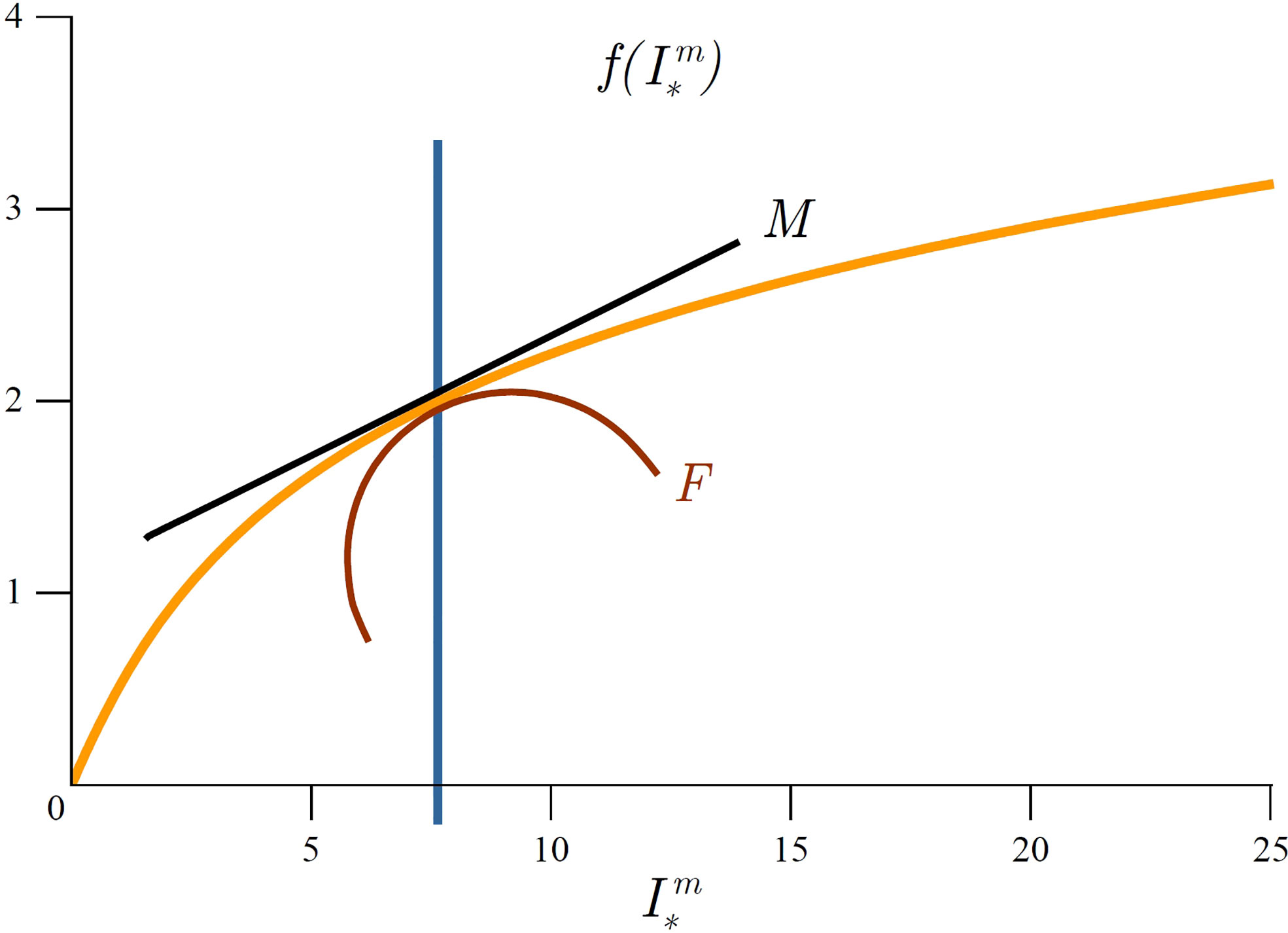
Figure 2 Graphical representation of marginal watercolumn production and watercolumn production fragility. The orange curve is the $f\left(I_{*}^m\right)$function (ordinate, dimensionless) from the canonical solution (10) for watercolumn production (Platt et al., 1990). Marginal watercolumn production M_I equals the first derivative of $f\left(I_{*}^m\right)$with respect to $I_{*}^m$ (black line). Watercolumn production fragility F_I equals the second derivative of $f\left(I_{*}^m\right)$ with respect to $I_{*}^m$ (red curve). $I_{*}^m$ is the scaled noon irradiance (dimensionless). As $I_{*}^m$ increases M_I declines and we say watercolumn production is fragile with respect to irradiance F_I< 0.

Following (4) we define marginal watercolumn production as:

$\begin{array}{ll}{M}_I=\frac{d{P}_{Z,T}}{d{I}_0^m}& (11)\end{array}$

which is measured in (mgCW^-1). Here noon irradiance is taken as representative of the watercolumn light conditions. To derive an exact expression for M₁ we begin with a prior result from Platt et al. (2017) (their equation 10):

$\begin{array}{ll}\frac{d{P}_{Z,T}}{d{I}_{*}^m}=\frac{B{P}_m^B}{K{I}_{*}^m}\underset{0}{\overset{D}{\int }}(1-\exp (-I_{*}^{m}g(t)))\text{d}t& (12)\end{array}$

which gives the change in watercolumn production P_Z,T with respect to $I_{*}^m$. By setting g(t)=sin (πt/D) , as used in our model, we get:

$\begin{array}{ll}\frac{d{P}_{Z,T}}{d{I}_{*}^m}=\frac{B{P}_m^B}{K{I}_{*}^m}\underset{0}{\overset{D}{\int }}(1-\exp (-I_{*}^m\sin (\pi t/D)))\text{d}t& (13)\end{array}$

The integral on the right hand side is recognized as surface production and is given by the analytical solution for the production profile:

$\begin{array}{ll}{P}_T(0)=B{P}_m^{B}D{f}_z(I_{*}^m)& (14)\end{array}$

where P_T(z) is the daily production at depth z and $f_z(I_{*}^m{e}^{-Kz})$ is a known function (Kovač et al., 2016a). Taking this solution into account transforms (13) into:

$\begin{array}{ll}\frac{d{P}_{Z,T}}{d{I}_{*}^m}=\frac{B{P}_m^{B}D}{K{I}_{*}^m}{f}_z(I_{*}^m)& (15)\end{array}$

By noting $\text{d}{I}_0^m=I_k \text{d}{I}_{*}^m$ the previous expression becomes:

$\begin{array}{ll}\frac{d{P}_{Z,T}}{d{I}_0^m}=\frac{P_T(0)}{K{I}_0^m}& (16)\end{array}$

and following (11) we recognize the result as marginal watercolumn production:

$\begin{array}{ll}{M}_I=\frac{P_T(0)}{K{I}_0^m}& (17)\end{array}$

Therefore, marginal watercolumn production M_I is proportional to surface production divided by the product of K and $I_0^m$ . Given that all the quantities on the right hand side are positive, marginal watercolumn production M_I is positive (Figure 2):

$\begin{array}{ll}{M}_I>0& (18)\end{array}$

Following (6) we define watercolumn production fragility:

$\begin{array}{ll}{F}_I=\frac{d{M}_I}{d{I}_0^m}& (19)\end{array}$

which is measured in (mg C m^-2 W^-2). To calculate F_I we take the derivative of (17) to get:

$\begin{array}{ll}{F}_I=\frac{1}{I_0^m}\left(\frac{1}{K}\frac{d{P}_T(0)}{d{I}_0^m}-M_I\right)& (20)\end{array}$

which is negative (Figure 2):

$\begin{array}{ll}{F}_I<0& (21)\end{array}$

implying watercolumn primary production is fragile with respect to surface irradiance.

Fragility being negative implies that fluctuations in surface irradiance will act to reduce mean primary production from what would otherwise result under steady surface irradiance. This further implies there is a lower limit on marginal watercolumn production:

$\begin{array}{ll}{M}_I>\frac{1}{K}\frac{d{P}_T(0)}{d{I}_0^m}& (22)\end{array}$

Visual interpretation of (18) and (21) is straightforward. In Figure 2 marginal production equals the first derivative of $f(I_{*}^m)$ with respect to $I_{*}^m$ and fragility equals the second derivative of $f(I_{*}^m)$ with respect to $I_{*}^m$. Ecological interpretation is also straightforward. As surface irradiance increases, light penetrates deeper into the watercolumn and production increases, but the rate of increase declines due to light saturation.

2.3 Mixed-layer production

Surface irradiance is not the only controlling factor of underwater light climate and consequently primary production. Typically, surface layer of the ocean has uniform properties up to a certain depth, termed the mixed-layer depth. In this layer phytoplankton are actively mixed (Franks, 2015) and experience uniform production, which is determined by surface irradiance and mixed-layer depth (Jackson et al., 2017). Therefore, mixed-layer depth variability has to be considered in a discussion of marginal production and fragility.

Let the depth of the mixed layer be given by Z_m and let P_Zm,T mark average mixed layer production (Figure 3), which following Kovač et al. (2020) equals:

$\begin{array}{ll}\langle P\rangle Z_m,T=\frac{B{P}_m^{B}D}{K{Z}_m}\left[f(I_{*}^m)-f(I_{*}^m{e}^{-K{Z}_m})\right]& (23)\end{array}$

We define marginal mixed-layer production as:

$\begin{array}{ll}{M}_Z=\frac{d\langle P\rangle Z_m,T}{d{Z}_m}& (24)\end{array}$

which quantifies the change in average mixed layer production caused by a change in mixed layer depth and is measured in in (mgCm⁻⁴). Following Kovač et al. (2020), due to light attenuation with depth, marginal mixed-layer production is lees than zero:

$\begin{array}{ll}{M}_Z<0& (25)\end{array}$

Simply stated, average mixed-layer production decreases with increasing mixed-layer depth (Figure 3). Further following Kovač et al. (2020) (their equation 71) we have:

$\begin{array}{ll}{M}_Z=\frac{1}{Z_m}\left[P_T(Z_m)-\langle PT(z)\rangle \right]& (26)\end{array}$

FIGURE 3

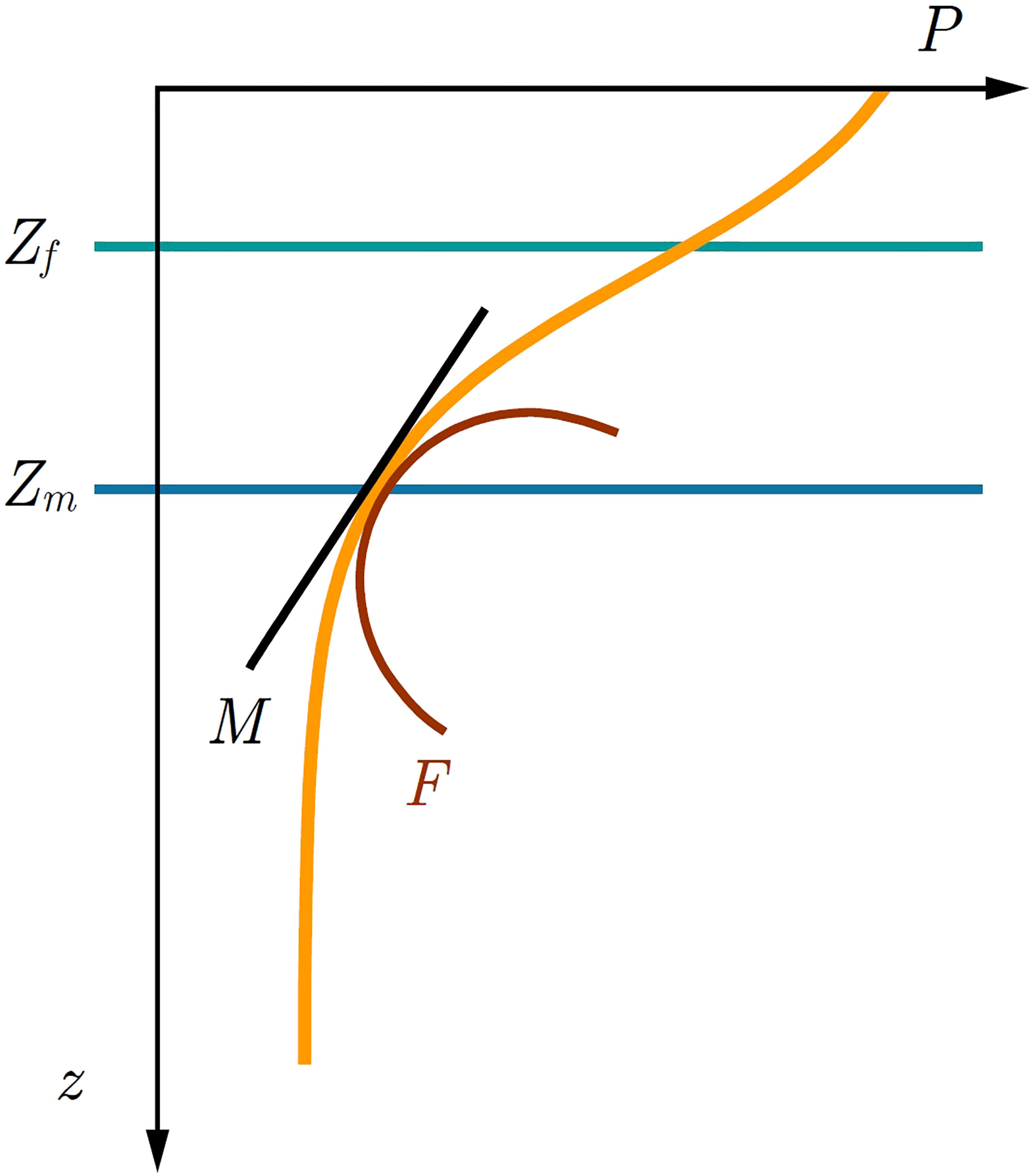
Figure 3 Graphical representation of marginal mixed-layer production and mixed-layer production fragility. Orange curve represents average mixed-layer production 〈P〉_Zm,_T as a function of depth (23). For a given mixed-layer depth Z_m (blue line) marginal production M_Z equals the first derivative of 〈P〉_Zm,_T with respect to Z_m and is indicated by the tangent (black line) and fragility is indicated by the curvature (red curve). Above Z_f (green line) the system is fragile, whereas below it the system is antifragile. Graphically, Z_f corresponds to the inflexion point and satisfies condition (31).

where P_T(Z_m) is the production at the mixed-layer base and 〈P_T(z)〉 is the average mixed layer production.

Having defined and expressed M_Z we now define mixed-layer production fragility F_Z as:

$\begin{array}{ll}{F}_Z=\frac{d{M}_Z}{d{Z}_m}& (27)\end{array}$

which is measured in (mgCm⁻⁵). Fragility due to mixed-layer depth variability quantifies the change in marginal production caused by a change in mixed-layer depth. Graphically, M_Z is the derivative of average mixed-layer production with depth and F_Z is the second derivative of average mixed-layer production with depth (Figure 3). Taking the derivative of (26) with respect to Z_m we get:

$\begin{array}{ll}{F}_Z=\frac{1}{Z_m}\left(\frac{d{P}_T(z)}{dz}{|}_{Z_m}-2M_Z\right)& (28)\end{array}$

Since ​dP_T(z)/​dz<0 (Kovač et al., 2016a) and M_Z<0 (25) the sign of F_Z can be positive, implying mixed-layer production could display antifragility, with variability in mixed-layer depth Z_m acting favourably on average mixed-layer production.

We term mixed-layer production fragile when mixed-layer deepening leads to a greater loss in average production, than the gain in production due to shallowing of the same magnitude. Mathematically we have:

$\begin{array}{ll}{F}_Z<0& (29)\end{array}$

We term mixed-layer production antifragile when mixed-layer deepening leads to a lesser loss in average production, than the gain in production due to shallowing of the same magnitude. Mathematically we have:

$\begin{array}{ll}{F}_Z>0& (30)\end{array}$

In contrast to watercolumn production fragility, mixed-layer production can be either fragile or antifragile. By considering F_Z=0 from (28) we get:

$\begin{array}{ll}\frac{d{P}_T(z)}{dz}{|}_Z=2M_Z& (31)\end{array}$

We term the depth at which this condition holds as the fragility depth Z_f as it represents the tipping point for primary production. Since fragility equals the first derivative of marginal production, zero fragility corresponds to an inflexion point of average mixed-layer production (Figure 3). At this depth marginal mixed-layer production has a minimum. If the mixed-layer depth is deeper than the fragility depth Z_m>Z_f , then mixed-layer variability acts favourably on primary production, whereas if the opposite holds (Z_m<Z_f) mixed-layer variability acts unfavourably on primary production.

3 Measurements

Here we use the available data from the Bermuda Atlantic Time-Series Study (BATS) and the Hawaii Ocean Time Series (HOT) to quantify marginal production and fragility. Both marginal production and fragility can be estimated directly from in situ measurements routinely done at these stations, which are comprised of: chlorophyll profile, production profile, attenuation coefficient and surface irradiance, all measured on a monthly basis. Complementary to these measurements, marginal production and fragility require information on the photosynthesis parameters. Following the methodology of Kovač et al. (2016b) these parameters were estimated from the aforementioned measurements, both at HOT (Kovač et al., 2016a) and BATS (Kovač et al., 2018) stations. More details on HOT data set can be found in Section 5 of Kovač et al. (2016a), whereas more details on the BATS data set can be found in Kovač et al. (2018).

We first quantified marginal watercolumn production M_I and watercolumn production fragility F_I , as derived in (17) and (20), respectively. The obtained values of M_I and F_I are shown in Figure 4 for both HOT and BATS. As expected, marginal watercolumn production is positive, whereas watercolumn fragility is negative. We then fitted the obtained values of F_I as a function of M_I . For HOT we obtained F_I=2.02−7.7M_I and for BATS F_I=2.05−9.1M_I . These relations help to quantify fragility from the knowledge of marginal production, which, following (17), can be computed from measurements of surface production, surface irradiance and the attenuation coefficient. Therefore, watercolumn fragility, as defined in (19), can be estimated from routine measurements for stations with a rich data archive, such as HOT and BATS.

FIGURE 4

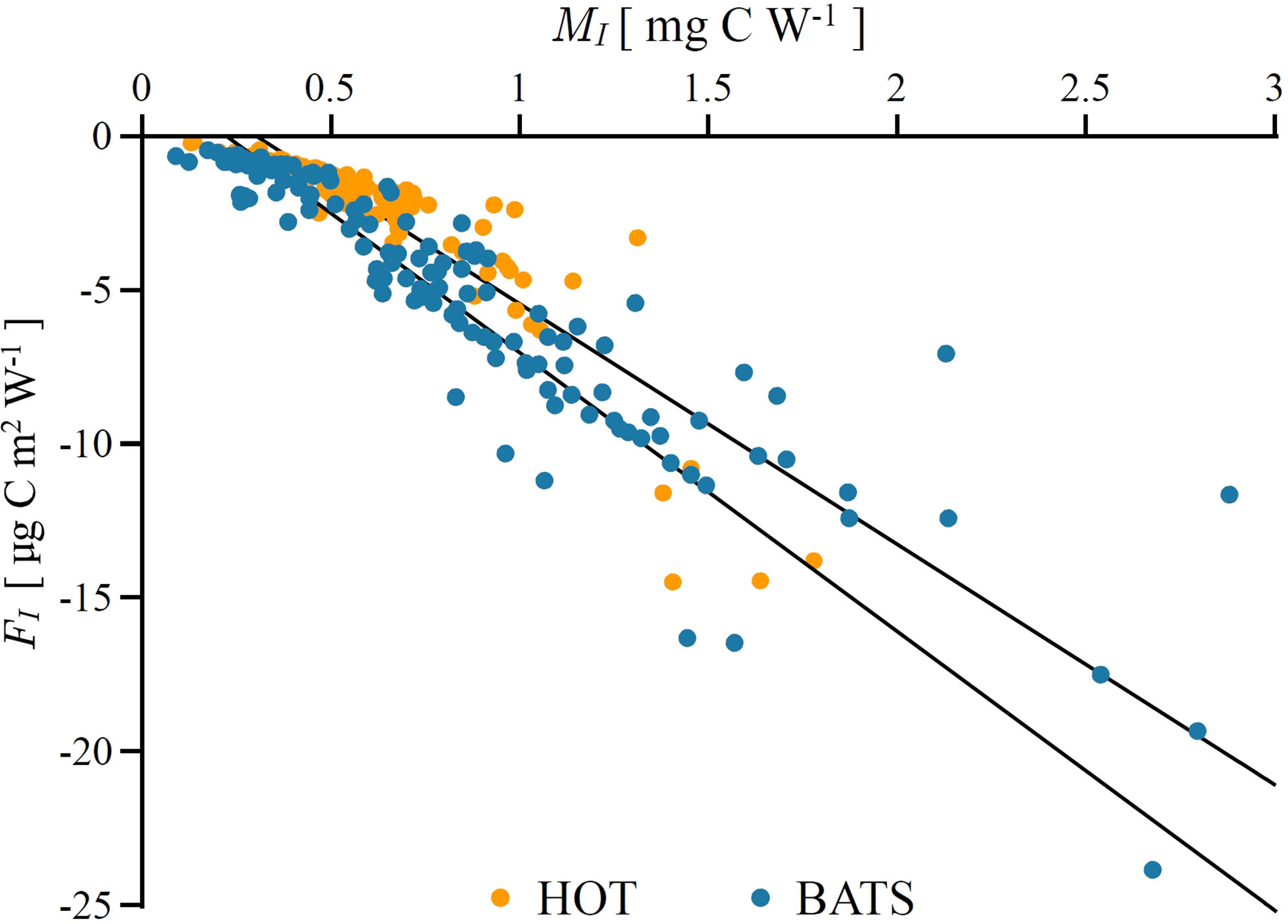
Figure 4 Marginal watercolumn production M_I and watercolumn production fragility F_I, as defined in (11) and (19), estimated from in situ data at Bermuda Atlantic Time-Series Study (blue dots) and Hawaii Ocean Time Series (orange dots). Black lines give a linear fit of F_I as a function of M_I for each station. All points are fragile implying variability in surface irradiance acts to suppresses biomass and production.

The estimated values of marginal mixed-layer production M_Z and mixed-layer production fragility F_Z , as derived in (26) and (28), are shown in Figure 5 for both HOT and BATS. As expected, following (25), marginal mixed-layer production is negative, whereas mixed-layer production fragility can be both negative or positive. This implies that at both stations primary production crosses the fragility tipping point as defined in (31). Histograms of Z_f are also shown in Figure 5. For HOT average Z_f equals 65 m with the standard deviation of 18 m. For BATS average Z_f equals 54 m with the standard deviation of 18 m. However, estimating marginal production and fragility from data only provides an insight into the instantaneous state of the system at the time of measurement. In order to provide a broader dynamical picture we now proceed to discuss how these concepts fit into a dynamical framework.

FIGURE 5

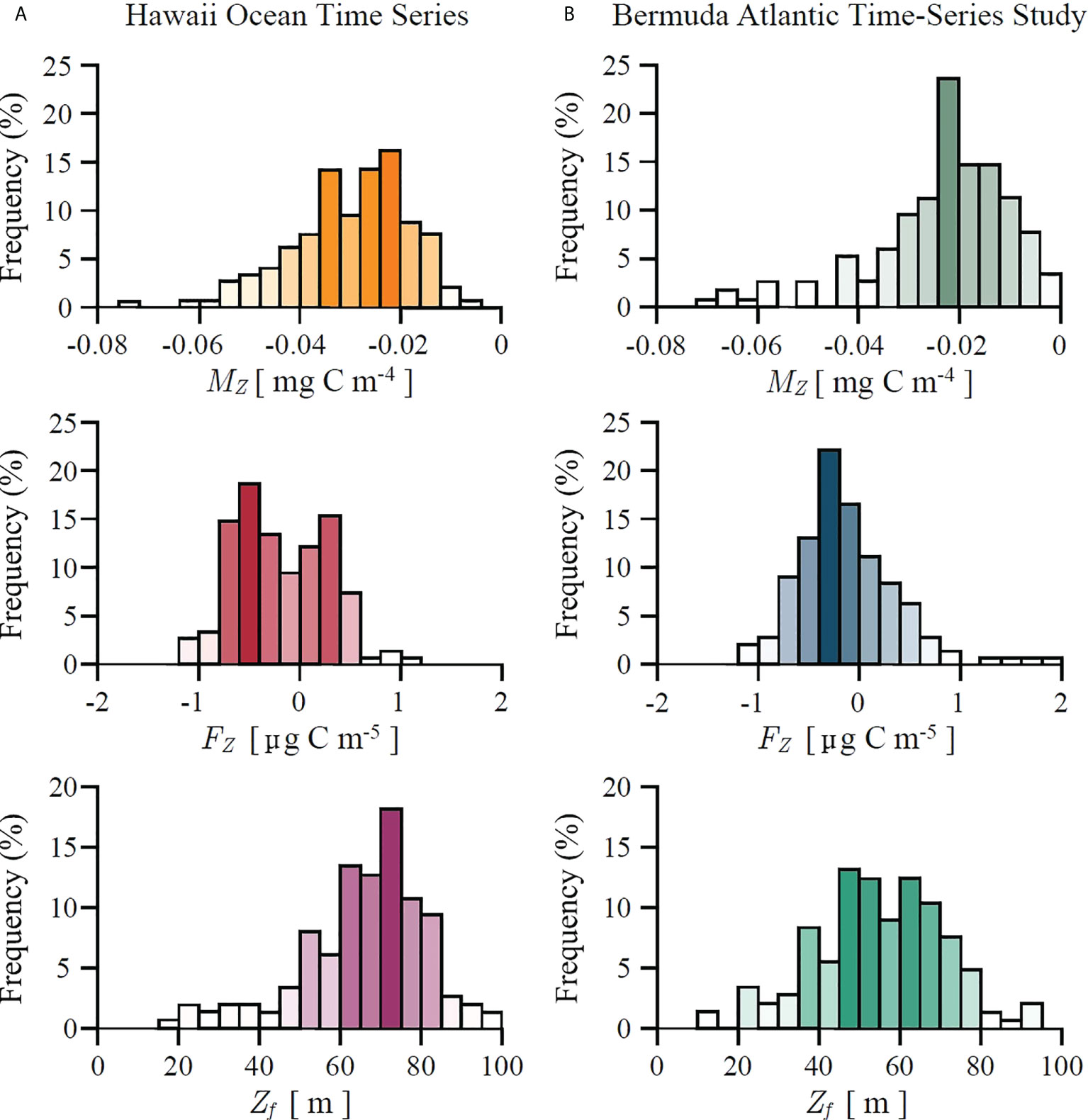
Figure 5 Histograms of marginal mixed-layer production M_Z, mixed-layer production fragility F_Z and fragility depth Z_f, as defined in (24), (27) and (31) respectively, estimated from in situ data at: (A) Hawaii Ocean Time Series and (B) Bermuda Atlantic Time-Series Study. At both stations marginal production M_Z is negative. Positive F_Z corresponds to antifragile states for which variability in mixed-layer depth acts favourably on biomass and production. Negative F_Z corresponds to fragile states for which variability in mixed-layer depth acts unfavourably on biomass and production. When the mixed-layer is shallower than Z_f the system is in a fragile state. When it is deeper than Z_f the system is in an antifragile state.

4 Dynamics

In order to demonstrate the effect of fragility on phytoplankton dynamics we place it in a dynamical context. Consider phytoplankton biomass in the mixed layer governed by the following equation (Platt et al., 2003a):

$\begin{array}{ll}B(t+1)=B(t)+\frac{1}{\chi }\langle P\rangle Z_m,T-L^{B}B(t)& (32)\end{array}$

where χ is the carbon-to-chlorophyll ratio and L^B is a generalized loss term. Time is discrete and B(t) marks biomass on day t=1,2,…N, where N is the simulation run time. We also include the effect of shading on the attenuation coefficient:

$\begin{array}{ll}K(t)=K_w+k_{B}B(t)& (33)\end{array}$

where K_w is the attenuation coefficient of sea water and k_B is the specific attenuation coefficient of phytoplankton (Kirk, 2011). Via (33) a bio-optical feedback is in effect, whereby increased biomass reduces light penetration, affecting mixed-layer production (23) and vice versa. Full list of parameters, their respective units and values used is provided in Table 1. We note that these values are not representative of HOT and BATS, but are based on previous literature values (Platt et al., 2003b; Edwards et al., 2004; Kovač et al., 2020) and serve to demonstrate the dynamical consequences of the introduced concepts via simulations. The code provided in the Supplementary material can be used to change parameter values and further explore the parameter space.

TABLE 1

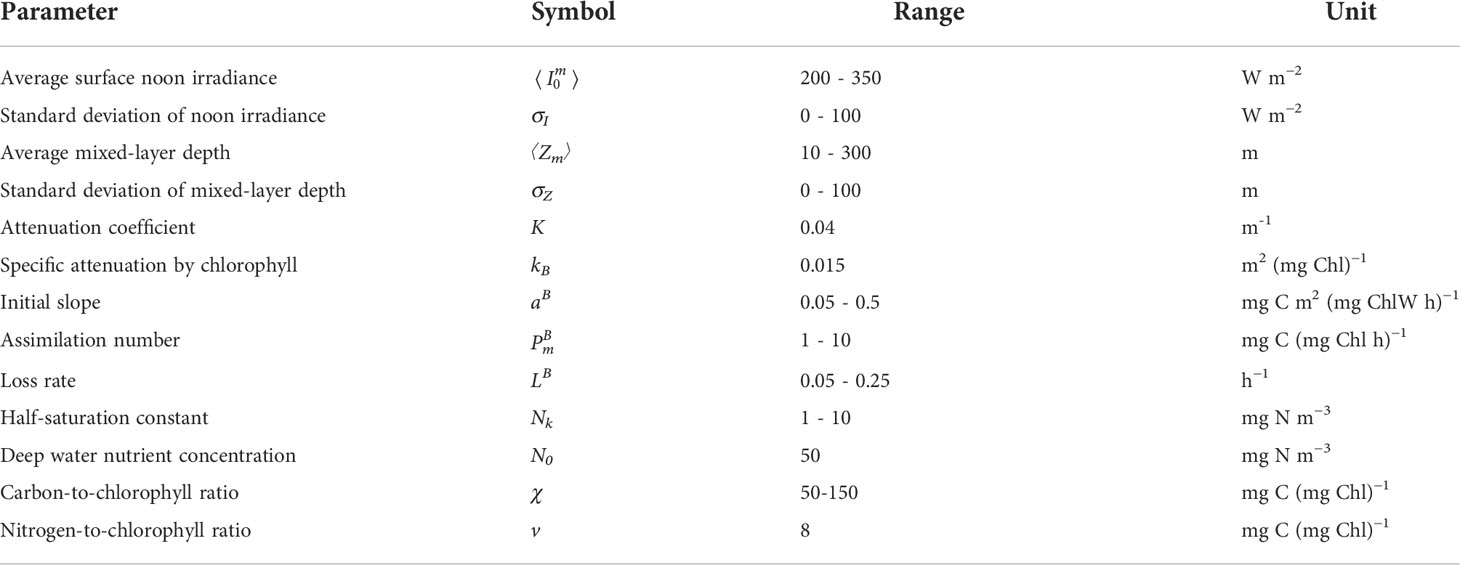
Table 1 Parameters and their typical values used in simulations.

The solution to this equation is either a trivial steady state biomass B^*=0 , when the loss term dominates, or a non-trivial steady state biomass B^*>0 , when the bio-optical feedback limits phytoplankton growth (Platt et al., 2003a; Edwards et al., 2004). At the non-trivial steady state production equals losses and therefore the critical depth, which by definition is the depth at which vertically integrated production equals losses (Sverdrup, 1953; Kovač et al., 2021), equals the mixed-layer depth. Upon mixed-layer depth change, the critical depth starts converging to the new mixed-layer depth, accompanied with a corresponding change in biomass, which now converges to the new steady state (Platt et al., 2003a; Edwards et al., 2004; Kovač et al., 2020).

However, this holds in a scenario where it is assumed that surface irradiance and mixed-layer depth are slowly varying in comparison to the growth rate of phytoplankton. Under these assumptions the phytoplankton have time to adjust to the new state after being perturbed, a condition that is hardly ever fulfilled in the real ocean, where variability in surface irradiance and mixed-layer depth is ever present. To take into account this variability, we model both surface irradiance and mixed-layer depth as random variables with a well-defined mean and normally distributed fluctuations. By doing so we explore the extent to which the notion of fragility is useful in explaining the response to rapid fluctuations. We expect that irradiance variability will induce unfavourable effects for phytoplankton biomass due to fragility (21). We also expect that mixed-layer variability could induce both favourable and unfavourable effects due to fragility and antifragility, indicated by (29) and (30).

4.1 Surface irradiance

To demonstrate these effects let us first consider surface irradiance of the form:

$\begin{array}{ll}{I}_0^m(t)=I_0^m+\delta I_0^m& (34)\end{array}$

where $I_0^m$is the average surface noon irradiance and $\delta I_0^m$is a normally distributed random variable with zero mean and standard deviation σ_I . Mixed-layer depth is held constant in order to first study the effect of surface irradiance variability. By integrating surface irradiance over time we get the average total received energy at the surface as:

$\begin{array}{ll}E=I_0^{m}T& (35)\end{array}$

where T is the interval of integration. Considering that the average total received energy is independent of the variability in surface irradiance one would naturally assume that the total realized production and therefore biomass would also be independent of the variably in surface irradiance. However, this is not the case.

Due to the non linear response of production to light, variability in surface irradiance acts to reduce the average realized biomass in the mixed layer, from what would otherwise result due to constant surface irradiance. In Figure 6 we provide an example model run to demonstrate this effect. Therefore, although on average the total received energy is the same, the realized biomass is not, demonstrating that primary production is indeed fragile with respect to surface irradiance (21). As the variability in surface irradiance σ_I increases, biomass declines still further.

FIGURE 6

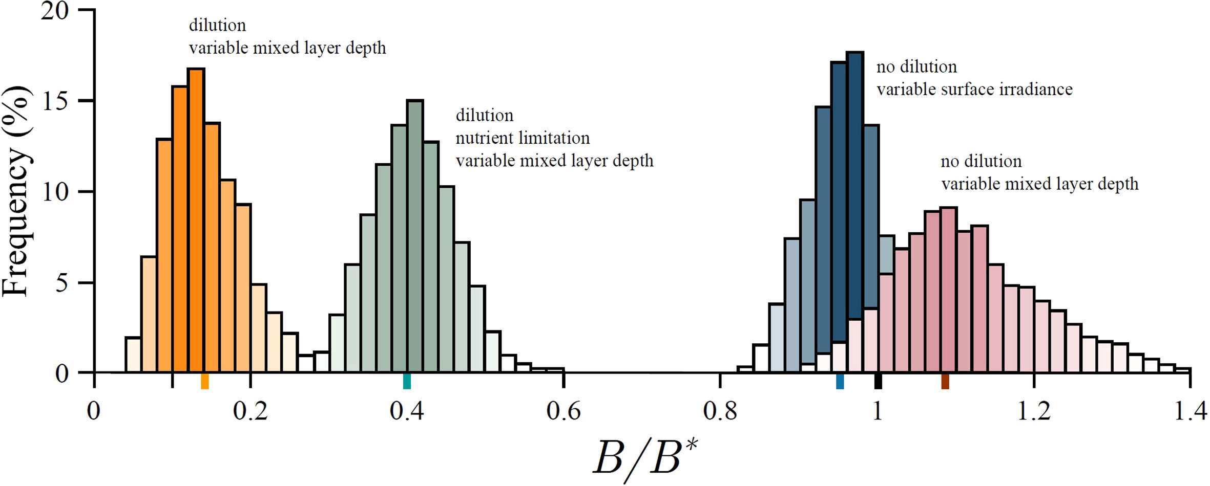
Figure 6 Distribution of the ratio of realized biomass B to the steady state biomass B^∗ for an example model run. Because of fragility biomass under variable surface irradiance (blue histogram) is on average lower (blue marker) than the steady state biomass under constant surface irradiance (black marker). In case of no dilution, and due to antifragility, biomass under variable mixed-layer depth (red histogram) is on average higher (red marker) than under constant mixed-layer depth (black marker). Taking dilution into account suppresses the biomass (orange histogram). However, taking dilution and nutrient limitation into account simultaneously raises the biomass from this suppressed state (green histogram). Average biomass for each scenario is given by the coloured marker on the abscissa. See Supplementary material for more information.

4.2 Mixed-layer depth

We now proceed to investigate fragility due to mixed-layer variability. In contrast to fragility due to irradiance variability, there are two possibilities: the system may be fragile or antifragile. We first provide an idealized case where deepening does not dilute mixed layer biomass. This is a reasonable assumption for the regions of the ocean with a deep chlorophyll maximum. Following the same procedure as for exploring the effect of the surface irradiance, we consider mixed-layer depth of the form:

$\begin{array}{ll}{Z}_m(t)=Z_m+\delta Z_m& (36)\end{array}$

where Z_m is the average mixed-layer depth and δZ_m is a normally distributed random variable with zero mean and standard deviation σ_Z . Surface irradiance is kept constant. In Figure 6 we provide an example model run where the average mixed-layer depth is greater than the fragility depth Z_m>Z_f (red histogram in Figure 6), therefore the system is in the antifragile state. As expected we notice an increase in biomass, from what would otherwise be obtained under constant mixed-layer depth.

To further explore the effect mixed-layer fragility has on biomass dynamics we extend equation (32) to include dilution as a consequence of mixed-layer deepening:

$\begin{array}{ll}B(t+1)=\left[B(t)+\frac{1}{\chi }{P}_{Z_m,T}-L^{B}B(t)\right]\frac{Z_m(t)}{Z_m(t+1)}& (37)\end{array}$

Dilution takes place in regions of the ocean where biomass is low below the mixed-layer. Here we set it equal to zero, to represent unfavourable growth conditions, a common assumption in the models of mixed layer dynamics (Edwards et al., 2004; Behrenfeld and Boss, 2014). Therefore, equation (32) holds for mixed-layer shallowing, whereas equation (37) holds for mixed-layer deepening. As the mixed-layer depth varies over time the system description alternates between these two equations.

During deepening there are two effects which work in unison to reduce biomass: dilution and production reduction due to reduced irradiance (caused by deepening under constant surface irradiance). During shallowing the production increase (due to increased average irradiance) acts to counterbalance the prior two effects. Results from an example model run are provided in Figure 6. In the figure we observe a biomass drop from a steady state value it would have otherwise achieved under constant or variable mixed-layer depth.

4.3 Nutrient concentration

To further investigate the dynamical effects of fragility on biomass and production we explicitly model the dependence of production on nutrients. Average mixed-layer production now becomes:

$\begin{array}{ll}\langle P\rangle Z_m,T=\frac{N}{N+N_k}\frac{B{P}_m^{B}D}{K{Z}_m}\left[f(I_0^m)-f(I_{*}^m{e}^{-K{Z}_m})\right]& (38)\end{array}$

where N stands for nutrients and N_k is the half-saturation constant for nutrient limitation (Kovač et al., 2020).We also explicitly model nutrient concentration N(t) during shallowing as:

$\begin{array}{ll}N(t+1)=N(t)-\frac{\nu }{\chi }{\mathrm{\langle P\rangle }}_{Z_m,T}& (39)\end{array}$

where ν is the nitrogen-to-chlorophyll ratio. During deepening, mixed-layer nutrient concentration increases due to entrainment and we have:

$\begin{array}{ll}N(t+1)=N(t)-\frac{\nu }{\chi }{\mathrm{\langle P\rangle }}_{Z_m,T}\frac{Z_m(t)}{Z_m(t+1)}+(N_0-N(t))\left(1-\frac{Z_m(t)}{Z_m(t+1)}\right)& (40)\end{array}$

where N₀ is the deep water nutrient pool. Therefore when Z_m(t+1)<Z_m(t) we employ (32) and (39), whereas when Z_m(t+1)>Z_m(t) we employ (37) and (40).

In Figure 6 we provide results from an example model run where the effects of biomass dilution and nutrient enrichment due to mixed-layer deepening are both taken into account. Now, deepening has an additional effect on average mixed-layer production: potential increase in production due to increased nutrients. This effect will manifest itself if the mixed-layer system is in a nutrient-limited state. In Figure 6 we observe an increase in biomass from what is observed under no nutrient limitation.

4.4 Seasonal cycle

So far we have analysed the response to variability in surface irradiance and mixed-layer depth, modelled by (34) and (36) around fixed mean values for both quantities. We next explore the effect of a seasonal cycle. We wish to investigate the change in dynamics resulting from crossing the fragility depth Z_f , which may occur sometime during the seasonal cycle. To model the crossing of Z_f we assume an annual cycle of mixed-layer depth with superimposed stochastic variability, of the form:

$\begin{array}{ll}{Z}_m(t)=Z_m^0+Z_m^a\cos (2\pi t/365)+\delta Z_m(t)& (41)\end{array}$

where now $Z_m^a$is the amplitude of the mixed-layer seasonal cycle. All other variables are the same as in (36). Likewise, for surface irradiance we assume:

$\begin{array}{ll}{I}_0^m(t)=I_0^m+I_0^a\cos (2\pi t/365)+\delta I_m^0& (42)\end{array}$

where now $I_0^a$is the amplitude of the surface irradiance seasonal cycle. Again, all other variables are the same as in (34).

A series of simulations of the seasonal cycle were performed. The model was run for up to 100 seasonal cycles. A typical result is provided in Figure 7, whereas longer model runs are provided in the Supplement. After the start of the simulation biomass quickly becomes phase locked to the seasonal cycle, dictated by mixed-layer depth and surface irradiance.,

However, the seasonal cycle in biomass becomes distorted as soon as the mixed-layer depth crosses the fragility depth (red arrow in Figure 7). The system entered the fragile regime at this point. The distortion is noticed as a drop in biomass over time (black arrow in Figure 7), which lasts until the system exits the fragile regime, which occurs when the mixed-layer depth becomes deeper than the fragility depth once again (orange arrow in Figure 7). The red and orange arrows only indicate the first and final times when F_z is negative and should not be confused with exact timing of the changes in system state due to stochastic variability in the variables. Although the variability in mixed-layer depth is constant over time it is amplified during the fragile regime, which is manifested in higher biomass variability. Mixed-layer fragility F_Z, defined in (27), correctly predicts the timing of this change in dynamics, namely by changing sign (Figure 7), highlighting that fragility is a good measure for quantifying these changes.

FIGURE 7

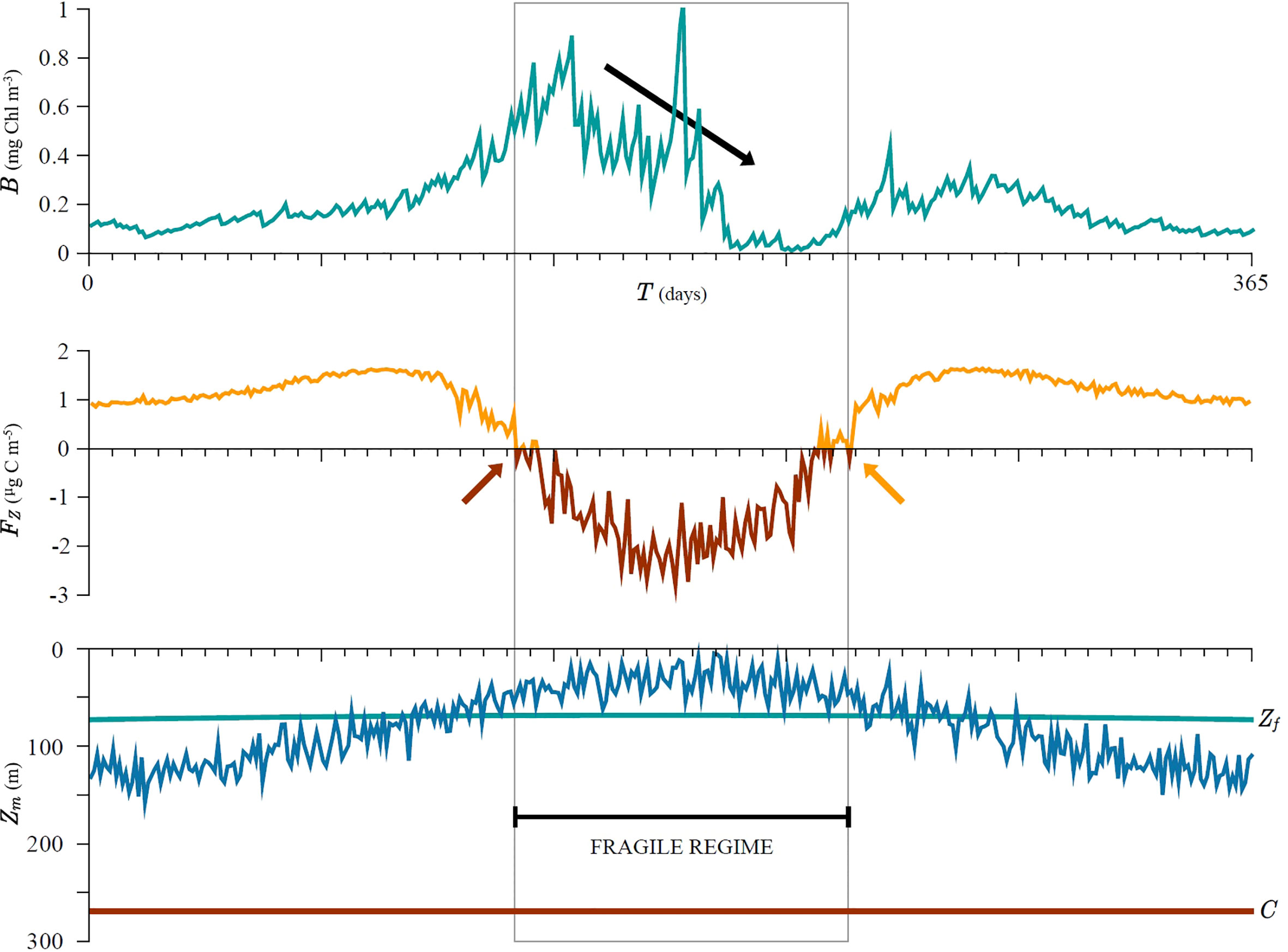
Figure 7 Simulated seasonal cycle of biomass, mixed layer depth and the resulting fragility. The seasonal cycle in biomass becomes distorted as soon as the mixed-layer depth (blue curve) crosses the fragility depth (green line). The distortion is noticed as a sharp drop in biomass over time (black arrow) which lasts until the system remains in the fragile state (grey area). Although the variability in mixed layer depth is constant over time it is amplified during the fragility regime and losses from dilution are harder to compensate by increased production from subsequent shallowing. The start and end of the fragility regime are correctly predicted as F_Z becomes negative and vice versa (orange and red curves/arrows). The critical depth C (red line) is deeper than the mixed-layer depth Z_m (blue curve) during the entire simulation, therefore the critical depth criterion is satisfied. See Supplementary material for more information.

We also observe that nutrient concentration remains high, but production and subsequently biomass decline (see Supplement), highlighting that the system naturally tends to a high nutrient low chlorophyll state, something that was also observed prior by Platt et al. (2003a) and Edwards et al. (2004). The production cycle also becomes distorted and acquires multiple seasonal peaks (see Supplement).

We wish to stress that during the whole model run the critical depth criterion is met, yet we notice a decline in biomass as a response to mixed-layer depth variability. This is a manifestation of fragility. In the beginning of the simulation mixed-layer depth is deeper than the fragility depth and the system is in an antifragile state with respect to mixed-layer variability. Therefore, after shallowing the relative gain in biomass can compensate the loss due to dilution from prior deepening and consequently biomass increases over time. Once the mixed-layer depth comes close to, or shallower than the fragility depth, the relative gain from shallowing can no longer compensate the loss from deepening and consequently biomass declines over time. The system entered the fragile state. Perhaps counter-intuitively, whilst the critical depth criterion is met the biomass can still decline due to fragility.

5 Discussion

The ocean ecosystem provides numerous societal services which are now under threat due to climate change (Henson et al., 2021). The socioeconomic value of the ocean ecosystem rests largely on the shoulders of phytoplankton primary production, the basis of the oceanic food web, which at present is estimated at 50 giga tons of carbon per year globally (Kulk et al., 2020; Kulk et al., 2021). The carbon assimilated in photosynthesis is transferred up the food chain, supporting fisheries, which consequently support the ever growing human population with food.

A sobering reminder that the consequences of changes in ecosystem functioning are not limited to the biological component of ecosystems alone and have socio-economical repercussions, are the crashes of Peruvian anchoveta and cod in Canada, which serve as stark reminders of the interplay between the ocean and the economy (Pauly et al., 2002). Arguably, if we are to build a sustainable blue economy, that keeps providing welfare to society, we should venture into thinking about phytoplankton as a productive system in an economic way and use the available economic theory to our advantage. As demonstrated in this work, using the economic concept of fragility enabled us to pinpoint a previously unknown tipping point for primary production.

At present, it is considered that one of the biggest threats ocean ecosystems face is posed by climate tipping points, critical thresholds after which perturbations irreversibly alter the dynamics of the system (Lenton et al., 2008; Lenton et al., 2019). Whereas physical tipping points in the ocean have been explored theoretically for some time now (Stommel, 1961; Weijer et al., 2019), the theoretical basis for tipping points in phytoplankton photosynthesis has not been well developed thus far. The stability of phytoplankton photosynthesis as a productive system has not been questioned on a theoretical basis, although numerous studies on climate change and phytoplankton have been published: Hays et al. (2005); Falkowski and Oliver (2007); Boyce et al. (2010), to name a few. Foremost, the tipping elements themselves have not been identified for phytoplankton prior to this work.

As we have demonstrated here, primary production is fragile with respect to surface irradiance (21) and both fragile and antifragile with respect to mixed-layer depth (29, 30). Fragility with respect to surface irradiance means that for the same amount of light energy received the average realized biomass in the mixed-layer is higher when surface irradiance is constant. For variable irradiance the realized biomass is lower. This highlights the significance of the fragility concept, as it grasps this asymmetry easily. Whereas the diurnal variability in surface irradiance under clear-sky conditions is fixed for a given location and day of year, and insensitive to climate change, the light available to phytoplankton could change with changes in clouds and to a lesser extent with storms and sea-surface roughness, which are indeed likely to be modified with climate change.

Similarly, for variable mixed-layer depth the realized biomass can be both higher or lower than the biomass corresponding to the constant mixed-layer depth. Higher than average biomass is associated with antifragility and lower with fragility. Antifragility is associated with deeper mixed layers and fragility with shallower mixed layers. Therefore, we demonstrated that variability acts favourably for biomass in deeper mixed layers and unfavourably for biomass in shallower mixed layers. Again, this may seem counter-intuitive, as one would expect phytoplankton to be more fragile in average low light due to greater mixed-layer depth. However, at low light any increase in light intensity is more favourable than at high light (as at low light, the photosynthetic response of phytoplankton to light available is a linear one). In economy this is the well known law of diminishing returns. Thought of it in this way the first photon is the most valuable, the second one less so, and so on.

It is important to note that although the concepts of fragility and antifragility did not come from the physical sphere, but rather from the economic one (Taleb, 2012), they were easily transferable to the biophysical models of primary production. Historically, the economic theory of capital has largely been incorporated into fisheries models for some time now (Schaefer, 1957; Clark, 1976; Clark et al., 1979). This is to be expected, since fisheries provide food and economic benefits for society. Unfortunately, the same line of reasoning has not been extended down the food web and economic theory of production has not yet been incorporated into marine primary production models. Here we have to distinguish the term primary production as used in oceanography, where it refers to carbon assimilation in phytoplankton photosynthesis, from the term production in fisheries economics, where it refers to the rate of harvesting.

Another more important distinction is the usage of theoretical terms in model structure. Economic theory as thus far used in fisheries literature augmented the biological theory by providing additional constraints and information on the optimal control of fisheries (Munro, 1992). In our work we have used economic insight to study a fundamental property of primary production in the pelagic ecosystem, namely fragility. The fragility property was hidden in the fundamental equations of primary production models, which rest on the photosynthesis light relation, represented by the photosyntehsis irradiance function (Platt and Jassby, 1976). It is at the level of the photosynthesis irradiance function that bio-physical coupling arises and consequently permeates to the ecosystem level by making watercolumn production either fragile or antifragile. Mathematically, the basic equations are non-autonomous and non-linear with respect to light which in turn makes these fragility effects possible.

Prior to this work fragility was an unrecognised property of marine primary production. Historically, stability of phytoplankton was viewed mostly through the lens of the Critical Depth Hypothesis (Lindeman and St. John, 2014; Sathyendranath et al., 2015; Behrenfeld and Boss, 2018). At its heart the Critical Depth Hypothesis, as mathematically formulated by Sverdrup (1953), asserts that mixed-layer phytoplankton biomass is sustainable if the critical depth surpasses the mixed-layer depth and vice versa (Figure 8). In their work Platt et al. (2003a) and Edwards et al. (2004) recognized the convergence of the critical depth to the mixed-layer depth and consequential suppression of biomass under stochastic forcing, which was stated as a potential explanation of the high nutrient low chlorophyll regions of the ocean. However, they only used two mixed-layer depths which consequently produced two steady states in biomass, a shallow and a deep state, and the system alternated between the two. Due to the bio-optical feedback the critical depth converged onto each mixed-layer depth and by doing so the biomass converged onto a steady state biomass. The deeper the mixed-layer the lower the biomass.

FIGURE 8

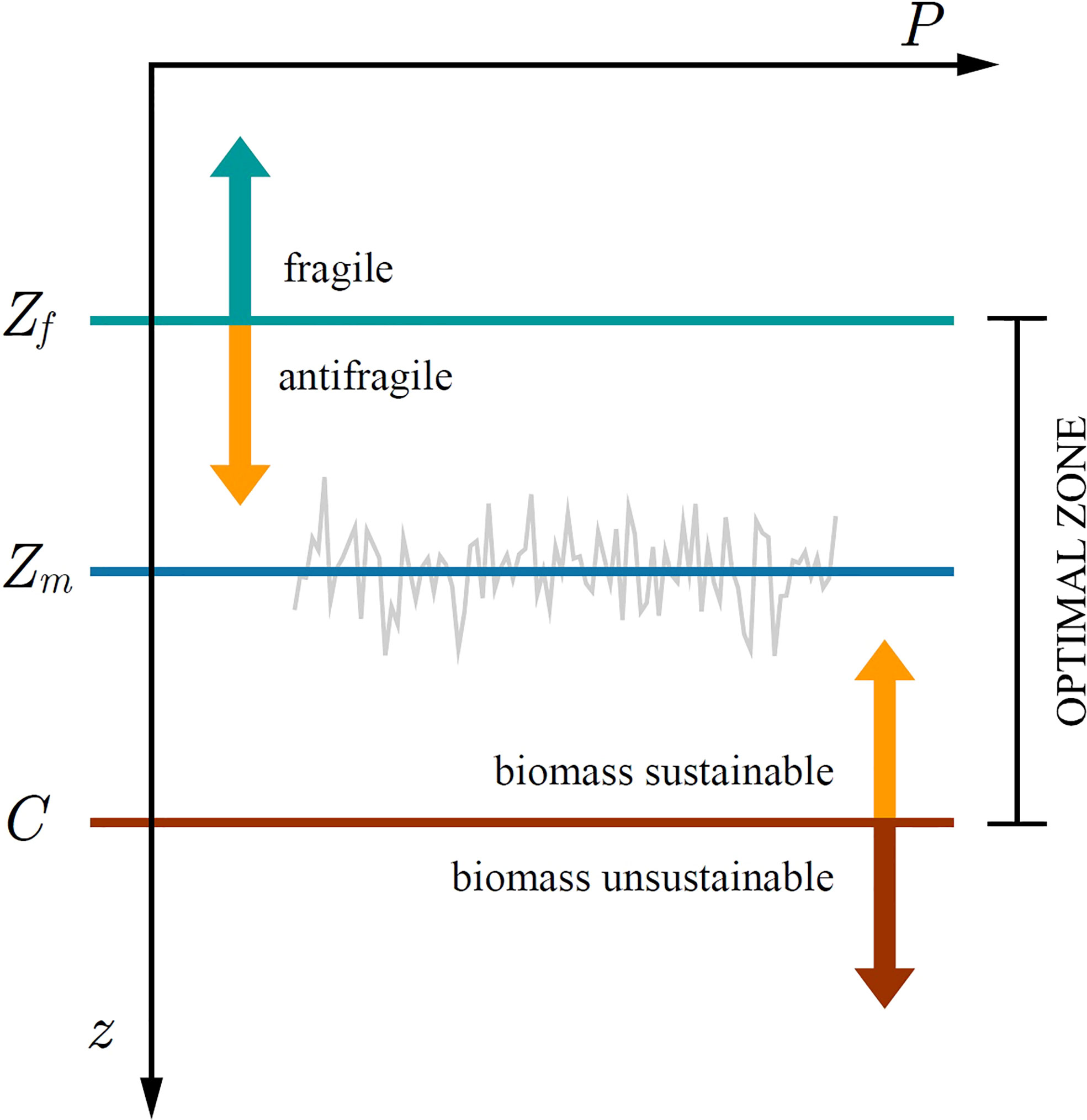
Figure 8 Illustration of the optimal zone for phytoplankton growth. At steady state the critical depth S converges onto the mixed layer depth Z_m. Below the optically uncoupled critical depth C biomass is unsustainable, whereas above C it is sustainable. Above the fragility depth Z_f phytoplankton biomass is suppressed from mixed-layer variability, whereas below Z_f it is increased. In the depth range from Z_f up to C phytoplankton can both be sustained and is antifragile to variability in mixed-layer depth.

Recently, Kovač et al. (2021) extended the Critical Depth Theory by redefining the critical depth as either: optically uncoupled critical depth C (phytoplankton shading not taken into account) and optically coupled critical depth S (phytoplankton shading taken into account). Kovač et al. (2021) demonstrated that the condition C>Z_m is necessary for the mixed-layer biomass to be sustained (Figure 8). In a sense, the optically uncoupled critical depth defines the carrying capacity for the biomass in the mixed-layer. Having met C>Z_m the sign of the growth rate is then determined by the difference between S and Z_m , with the biomass converging onto a steady state B^*. However, upon adding perturbations in the form of δZ_m the picture changes, as now the steady state biomass is either increased or suppressed, depending on the difference between Z_m and Z_f , where we recognize Z_f as a new depth horizon defined in (31). For mixed layers deeper than Z_f fragility acts favourably, whereas for mixed layers shallower than Z_f variability acts unfavourably. Below the fragility depth and above the optically uncoupled critical depth primary production can be sustained and is antifragile to perturbations in the mixed-layer depth (Figure 8).

Therefore, we conclude there is an optimal zone for the phytoplankton to thrive. If the mixed-layer depth is greater than the tipping depth and shallower than the optically uncoupled critical depth, variability acts favourably on primary production and consequently biomass. If the mixed-layer depth is shallower than the tipping depth, variability acts unfavourably on primary production and consequently biomass, regardless of the fact that it is shallower than the optically uncoupled critical depth. Even though the critical depth criterion is met, biomass can be suppressed due to variability in mixed-layer depth. Sverdrup’s critical depth criterion remains a necessary condition for initiation of phytoplankton blooms. However, it may not be a sufficient condition, as noted by Platt et al. (1991). Fragility arising from fluctuations in the light or nutrient field would add an additional argument in support of that statement.

We should stress that this behaviour would not have been observed if we had not used a non-linear production light relationship, such as (9). If a linear production light relationship of the form p^B(I)=α^BI was used, the model would display neither fragile nor antifragile behaviour with respect to surface irradiance, since it would respond linearly to surface irradiance. It would however display only antifragility with respect to mixed-layer depth, the reason being that the average mixed-layer production is a positively curved strictly declining function of depth for a linear photosynthesis irradiance function and therefore does not exhibit fragility, but only antifragility. In this case the fragility depth Z_f equals zero. This implies mixed-layer production fragility is a consequence of production saturation. Therefore, when modelling photosynthesis it is important to use a proper description of the photosynthesis-light relationship, as the effect of fragility will only manifest in the case of a saturating photosynthesis irradiance function.

Other important aspects that were not taken into account are photoinhibition and photoadaptation. In case of photoinhibiton the condition of marginal production being positive (5) would cease to hold after certain light intensities. This would split the photosynthesis irradiance function into two regimes: fragile and antifragile. However, in the ocean photoinhibition takes place close to the surface and in most waters does not have a strong effect on total watercolumn production. Similarly, photoadaptation should also have an effect on marginal production and fragility, as due to photoadaptation phytoplankton may alter its photosynthesis parameters to adapt to the ambient light, and therefore directly change the magnitude of marginal production and fragility. Exploring the effect of photoinhibition and photoadaptation on fragility is straightforward mathematically in the framework presented in this work. Both are plausible courses for future research.

6 Conclusions

The theory of ocean primary production has to a large extent survived untouched by the economic theory of production. As demonstrated in this paper, economic consideration of fragility has landed on fertile grounds in case of primary production. An economic concept of antifragility (Taleb, 2012) provided new insight into the biophysical system dynamics and revealed nuanced stability properties of phytoplankton photosynthesis. Going further, the economic theory of production and the biophysical theory of ocean primary production could benefit from stronger exchange of ideas, primarily with the goal of ocean conservation. Great care must be directed towards not flipping ocean primary production into a fragile regime and we must be careful that in our pursuit of a sustainable economy we do not make oceanic production, the base of oceanic economy, unsustainable due to our lack of knowledge about the system. The response of primary production to environmental perturbations needs to be explored in more detail and placed on firmer theoretical grounds if we are to understand the threats faced by the pelagic ecosystem in the near future. With this respect, investigating the differences between fragile and antifragile states at HOT and BATS would be a potential course for future research.

Data availability statement

Publicly available datasets were analyzed in this study. This data can be found here: https://hahana.soest.hawaii.edu/hot/hot-dogs/interface.html http://www.oceancolor.ucsb.edu/bbop

Author contributions

ŽK had the original idea. ŽK and SS formulated the mathematical model. ŽK derived the analytical expressions and implemented the model on the data sets. ŽK and SS wrote the original draft, both provided critical reviews and commentary on the draft, and wrote the final manuscript. All authors contributed to the article and approved the submitted version.

Funding

This work was supported by the Simons Collaboration on Computational Biogeochemical Modeling of Marine Ecosystems/CBIOMES (549947). This work is also a contribution to the Ocean-Colour Climate Change Initiative (OC-CCI) and the Biological Pump and Carbon Export Processes (BICEP) project of the European Space Agency. This work is a part of the activities of the National Centre for Earth Observations of the Natural Environmental Research council of the UK. This work has been supported in part by Croatian Science Foundation under the project MAUD (9849).

Conflict of interest

The authors declare that the research was conducted in the absence of any commercial or financial relationships that could be construed as a potential conflict of interest.

Publisher’s note

All claims expressed in this article are solely those of the authors and do not necessarily represent those of their affiliated organizations, or those of the publisher, the editors and the reviewers. Any product that may be evaluated in this article, or claim that may be made by its manufacturer, is not guaranteed or endorsed by the publisher.

Supplementary material

The Supplementary Material for this article can be found online at: https://www.frontiersin.org/articles/10.3389/fmars.2022.963395/full#supplementary-material

References

Acemoglu D. (2009). Introduction to modern economic growth. 1st ed (New Jersey, USA:University Press).

Google Scholar

Behrenfeld M. J., Boss E. S. (2014). Resurrecting the ecological underpinnings of ocean plankton blooms. Annu. Rev. Mar. Sci. 6, 167–194. doi: 10.1146/annurev-marine-052913-021325

CrossRef Full Text | Google Scholar

Behrenfeld M. J., Boss E. S. (2018). Student’s tutorial on bloom hypotheses in the context of phytoplankton annual cycles. Global Change Biol. 24, 55–77. doi: 10.1111/gcb.13858

CrossRef Full Text | Google Scholar

Boyce D. G., Lewis M. R., Worm B. (2010). Global phytoplankton decline over the past century. Nature 466, 591–596. doi: 10.1038/nature09268

PubMed Abstract | CrossRef Full Text | Google Scholar

Clark C. W. (1976). Mathematical bioeconomics (New Jersey, USA:Wiley-Interscience).

Google Scholar

Clark C. W., Clarke F. H., Munro G. R. (1979). The optimal exploitation of renewable resource stocks: Problems of irreversible investment. Econometrica 47 (1), 25–47. doi: 10.2307/1912344

CrossRef Full Text | Google Scholar

Clark C. W., Munro G. R. (1975). The economics of fishing and modern capital theory: A simplified approach. J. Environ. Economics Manage. 2, 92–106. doi: 10.1016/0095-0696(75)90002-9

CrossRef Full Text | Google Scholar

Da N., Foltz G. R., Balaguru K. (2021). Observed global increases in tropical cyclone-induced ocean cooling and primary production. Geophys. Res. Lett. 48, e2021GL092574. doi: 10.1029/2021GL092574

CrossRef Full Text | Google Scholar

Edwards A. E., Platt T., Sathyendranath S. (2004). The high-nutrient, low-chlorophyll regime of the ocean: limits on biomass and nitrate before and after iron enrichment. Ecol. Model. 171, 103–125. doi: 10.1016/j.ecolmodel.2003.06.001

CrossRef Full Text | Google Scholar

Falkowski P. G., Oliver M. J. (2007). The power of plankton. Nat. Rev. Microbiol. 5, 813–819. doi: 10.1038/nrmicro1751

PubMed Abstract | CrossRef Full Text | Google Scholar

Franks P. J. S. (2015). Has sverdrup’s critical depth hypothesis been tested? mixed layers vs. turbulent layers. ICES J. Mar. Sci. 72, 1897–1907. doi: 10.1093/icesjms/fsu175

CrossRef Full Text | Google Scholar

Frölicher T., Rodgers K. B., Stock C. A., Ceung W. W. L. (2016). Sources of uncertainties in 21st century projections of potential ocean ecosystem stressors. Global Biogeochem. Cycles 30, 1224–1243. doi: 10.1002/2015GB005338

CrossRef Full Text | Google Scholar

Hays G., Richardson A. J., Robinson C. (2005). Climate change and marine plankton. Trends Ecol. Evol. 20 (6), 337–344. doi: 10.1016/j.tree.2005.03.004

PubMed Abstract | CrossRef Full Text | Google Scholar

Henson S. A., Cael B. B., Allen S. R., Dutkiewicz S. (2021). Future phytoplankton diversity in a changing climate. Nat. Commun. 12, 5372. doi: 10.1038/s41467-021-25699-w

PubMed Abstract | CrossRef Full Text | Google Scholar

Jackson T., Sathyendranath S., Platt T. (2017). An exact solution for modeling photoacclimation of the carbon-to-chlorophyll ratio in phytoplankton. Front. Mar. Sci. 4, 283. doi: 10.3389/fmars.2017.00283

CrossRef Full Text | Google Scholar

Jassby A. D., Platt T. (1976). Mathematical formulation of the relationship between photosynthesis and light for phytoplankton. Limnol. Oceanogr. 21, 540–547. doi: 10.4319/lo.1976.21.4.0540

CrossRef Full Text | Google Scholar

Jones C. T., Craig S. E., Barnett A. B., MacIntyre H. L., Cullen J. J. (2014). Curvature in models of the photosynthesis-irradiance response. J. Phycol. 50, 341–355. doi: 10.1111/jpy.12164

PubMed Abstract | CrossRef Full Text | Google Scholar

Kirk J. T. O. (2011). Light and photosynthesis in quatic ecosystems. 3rd ed (Cambridge, UK:Cambridge University Press).

Google Scholar

Kovač Ž., Platt T., S. S., Antunović S. (2017). Models for estimating photosynthesis parameters from in situ production profiles. Prog. Oceanogr. 159, 255–266. doi: 10.1016/j.pocean.2017.10.013

CrossRef Full Text | Google Scholar

Kovač Ž., Platt T., Sathyendranath S. (2020). Stability and resilience in a nutrient-phytoplankton marine ecosystem model. ICES J. Mar. Sci. 77 (4), 1556–1572. doi: 10.1093/icesjms/fsaa067

CrossRef Full Text | Google Scholar

Kovač Ž., Platt T., Sathyendranath S. (2021). Sverdrup meets lambert: analytical solution for sverdrup’s critical depth. ICES J. Mar. Sci. fsab013, 78(4), 1398–1408. doi: 10.1093/icesjms/fsab013

CrossRef Full Text | Google Scholar

Kovač Ž., Platt T., Sathyendranath S., Morović M., Jackson T. (2016b). Recovery of photosynthesis parameters from in situ profiles of phytoplankton production. ICES J. Mar. Sci. 73 (2), 275–285. doi: 10.1093/icesjms/fsv204

CrossRef Full Text | Google Scholar

Kovač Ž., Platt T., Sathyendranath S., Morović M., Lomas M. W. (2018). Extraction of photosynthesis parameters from time series measurements of in situ production: Bermuda atlantic time-series study. Remote Sens. 10, 1–23. doi: 10.3390/rs10060915

CrossRef Full Text | Google Scholar

Kovač Ž., Platt T., S. S., Morović M. (2016a). Analytical solution for the vertical profile of daily production in the ocean. J. Geophys. Res.: Oceans 121. doi: 10.1002/2015JC011293

CrossRef Full Text | Google Scholar

Kulk G., Platt T., Dingle J., Jackson T., Johnsson B., Bouman H. A., et al. (2020). Primary production, an index of climate change in the ocean: Satellite-based estimates over two decades. Remote Sens. 12 (5), 826. doi: 10.3390/rs12050826

CrossRef Full Text | Google Scholar

Kulk G., Platt T., Dingle J., Jackson T., Johnsson B., Bouman H. A., et al. (2021). Correction: Primary production, an index of climate change in the ocean: Satellite-based estimates over two decades. Remote Sens. 13 (17), 3462.

Google Scholar

Kwiatkowski L., Torres O., Bopp L., Aumont O., Chamberlain M., Christian J. R., et al. (2020). Twenty-first century ocean warming, acidification, deoxygenation, and upper-ocean nutrient and primary production decline from cmip6 model projections. Biogeosciences 17, 3439–3470. doi: 10.5194/bg-17-3439-2020

CrossRef Full Text | Google Scholar

Laufkötter C., Vogt M., Gruber N., Aita-Noguchi M., Aumont O., Bopp L., et al. (2015). Drivers and uncertainties of future global marine primary production in marine ecosystem models. Biogeosciences 12, 6955–6984. doi: 10.5194/bg-12-6955-2015

CrossRef Full Text | Google Scholar

Lenton T. M., Held H., Kriegler E., Hall J. W., Lucht W., Rahmstorf S., et al. (2008). Tipping elements in the earth’s climate system. Proc. Natl. Acad. Sci. 105, 1786–1793. doi: 10.1073/pnas.0705414105

CrossRef Full Text | Google Scholar

Lenton T., Rockstrom J., Gaffney O., Rahmstorf S., Richardson K., Steffen W., et al. (2019). Climate tipping points - too risky to bet against. Nature 575, 592–595. doi: 10.1038/d41586-019-03595-0

PubMed Abstract | CrossRef Full Text | Google Scholar

Lindeman C., St. John M. A. (2014). A seasonal diary of phytoplankton in the north atlantic. Front. Mar. Sci. 1 (37), 1–6. doi: 10.3389/fmars.2014.00037

CrossRef Full Text | Google Scholar

Longhurst A., Sathyendranath S., Platt T. (1995). An estimate of global primary production in the ocean from satellite radiometer data. J. Plankton Res. 17, 1245–1271. doi: 10.1093/plankt/17.6.1245

CrossRef Full Text | Google Scholar

Munro G. R. (1992). Mathematical bioeconomics and the evolution of modern fisheries economics. Bull. Math. Biol. 54 (2/3), 163–184. doi: 10.1016/S0092-8240(05)80021-7

PubMed Abstract | CrossRef Full Text | Google Scholar

Pauly D., Christensen V., Guenette S., Pitcher T. J., Sumila U. R., Walters C. J., et al. (2002). Towards sustainability in world fisheries. Nature 418, 689–695. doi: 10.1038/nature01017

PubMed Abstract | CrossRef Full Text | Google Scholar

Perman R., Ma Y., Common M., Maddison D., McGilvray J. (2011). Natural resource and environmental economics. 4th ed (Gosport, UK:Pearson Education Limited).

Google Scholar

Platt T., Bird D. F., Sathyendranath S. (1991). Critical depth and marine primary production. Proc. R. Soc. B 246, 205–217. doi: 10.1098/rspb.1991.0146

CrossRef Full Text | Google Scholar

Platt T., Broomhead D. S., Sathyendranath S., Edwards A. M., Murphy E. J. (2003a). Phytoplankton biomass and residual nitrate in the pelagic ecosystem. Proc. R. Soc. A 459, 1063–1073. doi: 10.1098/rspa.2002.1079

CrossRef Full Text | Google Scholar

Platt T., Gallegos C. L., Harrison W. G. (1980). Photoinhibition of photosynthesis in natural assemblages of marine phytoplankton. J. Mar. Res. 38, 687–701.

Google Scholar

Platt T., Jassby A. (1976). The relationship between photosynthesis and light for natural assemblages of coastal marine phytoplankton. J. Phycol. 12, 421–430. doi: 10.1111/j.1529-8817.1976.tb02866.x

CrossRef Full Text | Google Scholar

Platt T., Sathyendranath S. (1988). Oceanic primary production: Estimation by remote sensing at local and regional scales. Science 241, 1613–1620. doi: 10.1126/science.241.4873.1613

PubMed Abstract | CrossRef Full Text | Google Scholar

Platt T., Sathyendranath S. (1991). Biological production models as elements of coupled, atmosphere-ocean models for climate research. J. Geophys. Res. 96, 2585–2592. doi: 10.1029/90JC02305

CrossRef Full Text | Google Scholar

Platt T., Sathyendranath S., Edwards A. M., Broomhead D. S., Ulloa O. (2003b). Nitrate supply and demand in the mixed layer of the ocean. Mar. Ecol. Prog. Ser. 254, 3–9. doi: 10.3354/meps254003

CrossRef Full Text | Google Scholar

Platt T., Sathyendranath S., Ravindran P. (1990). Primary production by phytoplankton: Analytic solutions for daily rates per unit area of water surface. Proc. R. Soc. B 241, 101–111. doi: 10.1098/rspb.1990.0072

CrossRef Full Text | Google Scholar

Platt T., Sythyendranath S., White G. N., Jackson T., Saux Picart S., Bouman H. (2017). Primary production: Sensitivity to surface irradiance and implications for archiving data. Front. Mar. Sci. 4, 387. doi: 10.3389/fmars.2017.00387

CrossRef Full Text | Google Scholar

Regaudie-de Gioux A., Lasternas S., Agusti S., Duarte C. M. (2014). Comparing marine primary production estimates through different methods and development of conversion equations. Front. Mar. Sci. 19), 1–14. doi: 10.3389/fmars.2014.00019

CrossRef Full Text | Google Scholar

Richmond P., Mimkes J., Hutzler S. (2013). Econophysics and physical economics. 1st ed (Oxford University Press).

Google Scholar

Sathyedranath S., Longhurst A., Caverhill C. M., Platt T. (1995). Regionally and seasonally differentiated primary production in the north Atlantic. Deep Sea Res. 1 42, 1773–1802. doi: 10.1016/0967-0637(95)00059-F

CrossRef Full Text | Google Scholar

Sathyendranath S., Ji R., Browman H. I. (2015). Revisiting sverdrup’s critical depth hypothesis. ICES J. Mar. Sci. 72, 1892–1896. doi: 10.1093/icesjms/fsv110

CrossRef Full Text | Google Scholar

Schaefer M. B. (1957). Some considerations of populatiorr dynarnics and economics in relation to the managernent of the commercial fisheries. J. Fish. Board Canada 14 (5), 669–681. doi: 10.1139/f57-025

CrossRef Full Text | Google Scholar

Stommel H. (1961). Thermohahe convection with two stable regimes of flow. Tellus 13, 224–230. doi: 10.3402/tellusa.v13i2.9491

CrossRef Full Text | Google Scholar

Sverdrup H. U. (1953). On conditions for the vernal blooming of phytoplankton. J. du Conseil Int. pour l’Exploration la Mer 18, 287–295.

Google Scholar

Taleb N. N. (2012). Antifragile: things that gain from disorder (United States:The Random House Publishing).

Google Scholar

Watson W. G., Rouusseaux C. S. (2019). Global ocean primary production trends in the modern ocean color satellite record, (1998–2015). Environ. Res. Lett. 14, 124011. doi: 10.1088/1748-9326/ab4667

CrossRef Full Text | Google Scholar

Weijer W., Cheng W., Drijfhout S. S., Fedorov A. V., Hu A., Jackson L. C., et al. (2019). Stability of the atlantic meridional overturning circulation: A review and synthesis. J. Geophys. Res.: Oceans 124 (8), 5336–5375. doi: 10.1029/2019JC015083

CrossRef Full Text | Google Scholar