Estimating abundance of an elusive cetacean in a complex environment: Harbor porpoises (Phocoena phocoena) in inland waters of Southeast Alaska

Introduction

Marine mammals are susceptible to anthropogenic threats, including incidental mortality in fisheries operations and habitat degradation (Reeves et al., 2013; Avila et al., 2018). Monitoring abundance and trends is critical to understanding the effect of these threats to their populations. The harbor porpoise (Phocoena phocoena) is one of the smallest cetaceans and is considered to be a sentinel species due to its sensitivity to many anthropogenic threats, including noise, fishery interactions, and habitat degradation (Read et al., 1997; Braulik et al., 2020; Carlén et al., 2021). This species is widely distributed in temperate waters of the Northern Hemisphere; typically in coastal environments (Read, 1999), but some individuals may occur in oceanic habitats (Nielsen et al., 2018). At a global level, the harbor porpoise is listed as “Least Concern” on the International Union for the Conservation of Nature (IUCN) Red List (Braulik et al., 2020), but some regional populations are believed to be at greater risk (Birkun and Frantzis, 2008; Hammond et al., 2008; Carlén et al., 2021).

Along the western coast of North America, from the waters off California to the Beaufort Sea in Alaska, multiple stocks of harbor porpoise are recognized (Carretta et al., 2019; Muto et al., 2020). Until recently, harbor porpoise in Southeast Alaska (SEAK) were considered part of a single stock that included porpoise in Yakutat Bay, open ocean areas of the Gulf of Alaska between approximately 55 and 60°N, and inland waters of SEAK (Muto et al., 2020). Analysis of sighting data from ship surveys conducted by the Marine Mammal Laboratory of NOAA’s Alaska Fisheries Science Center (MML/AFSC) between 1991 and 2012 suggested that numbers of harbor porpoise in the northern portion of the inland waters were stable. However, in the southern portion, numbers declined significantly in the mid-2000s and increased again in early 2010 (Dahlheim et al., 2015). The decline was observed in a region where the salmon drift gillnet fisheries operate (Manly, 2015). Such contrasting trends in abundance between the northern and southern portions of SEAK inland waters suggested that substructure exists within the SEAK harbor porpoise stock. Subsequently, genetic analysis, based on tissue and environmental DNA (e-DNA), provided evidence of at least two areas where harbor porpoise are genetically differentiated within the inland waters of SEAK (Parsons et al., 2018; Parsons et al., 2021). Information on distribution patterns, trends in abundance, and genetics led to the recognition of two demographically independent populations (DIPs) in inland waters of SEAK, the northern (N-SEAK) and southern (S-SEAK) Southeast Alaska inland water DIPs (Zerbini et al., 2022). It is likely that multiple DIPs exist within the remaining SEAK harbor porpoise stock, including porpoise in Yakutat Bay, and along the SEAK outer coast and offshore waters. However, as there is insufficient data to delineate units within that area, harbor porpoise were grouped into a single unit called the Yakutat/Southeast Alaska Offshore Waters unit (Zerbini et al., 2022). Currently, the US government is in the process of recognizing the N-SEAK and the S-SEAK DIPs and the Yakutat/SEAK Offshore unit as three separate stocks.

There is evidence that incidental mortality of harbor porpoise in the salmon drift gillnet fishery in SEAK inland waters may exceed the maximum allowable level under the United States Marine Mammal Protection Act (MMPA) (Muto et al., 2018). The most recent estimates of harbor porpoise abundance for the whole of SEAK (Hobbs and Waite, 2010) and for SEAK inland waters (Dahlheim et al., 2015) are more than eight years old and considered outdated for use in management under the MMPA (Angliss and Wade, 1997). Therefore, a new estimate is needed to update estimates of the potential impact of bycatch on SEAK harbor porpoise.

Developing statistically robust abundance surveys in inland waters of SEAK is challenging because of the region’s complex geography, consisting of a network of open waterways interspersed by hundreds of islands, narrow fjords, and inlets. The inland waters of SEAK correspond to the northern terminus of the Inside Passage, which also includes the northern coastal waters of Washington State in the US and the coast of British Columbia in Canada. This relatively protected and complex region provides important habitats for many cetacean species (Dahlheim et al., 2009), but it is difficult and expensive to design surveys that sample all possible habitats.

Here, we describe the results of a ship survey developed using a combination of line- and strip-transect methods to sample different habitats in SEAK inland waters in the summer 2019. The main goal of the survey was to assess distribution and to compute new density and abundance estimates for N-SEAK and S-SEAK harbor porpoise DIPs in inland waters. These estimates are discussed in the context of the estimated human-induced mortality in the region and the potential conservation consequences for a cetacean species widely known to be vulnerable to entanglements in fishing gear.

Methods

Study area and survey design

The study area encompassed inland waters of SEAK from Cross Sound in the north to Dixon Entrance in the south (Figure 1), a region of 23,821 km². The survey only covered the range of the two SEAK harbor porpoise DIPs within inland waters. None of the habitats in the Yakutat/Southeast Alaska Offshore waters unit was sampled during this cruise. Allocation of sampling transects followed concepts presented in Thomas et al. (2007) who provided a framework to design a line-transect survey along the coast of BC, an area with complex features similar to SEAK. We designed the present survey to meet the following objectives:

● Obtain an approximately uniform sampling coverage of the study area;

● Sample all areas previously surveyed by MML cruises to allow for spatial comparability across surveys and for future estimation of trends in abundance;

● Account for loss of survey effort due to unfavorable weather (previous surveys indicated that ~25-35% of the survey days were lost due to inclement weather in the region) and for transiting between tracklines and survey regions;

● Survey all areas in SEAK inland waters where the salmon driftnet fishery operates;

● Sample areas within SEAK inland where harbor porpoises are believed to occur but were not surveyed in previous years;

● Optimize survey effort given the allocated survey period;

● Exclude regions where navigation is restricted given the size of the ship and water depth.

FIGURE 1

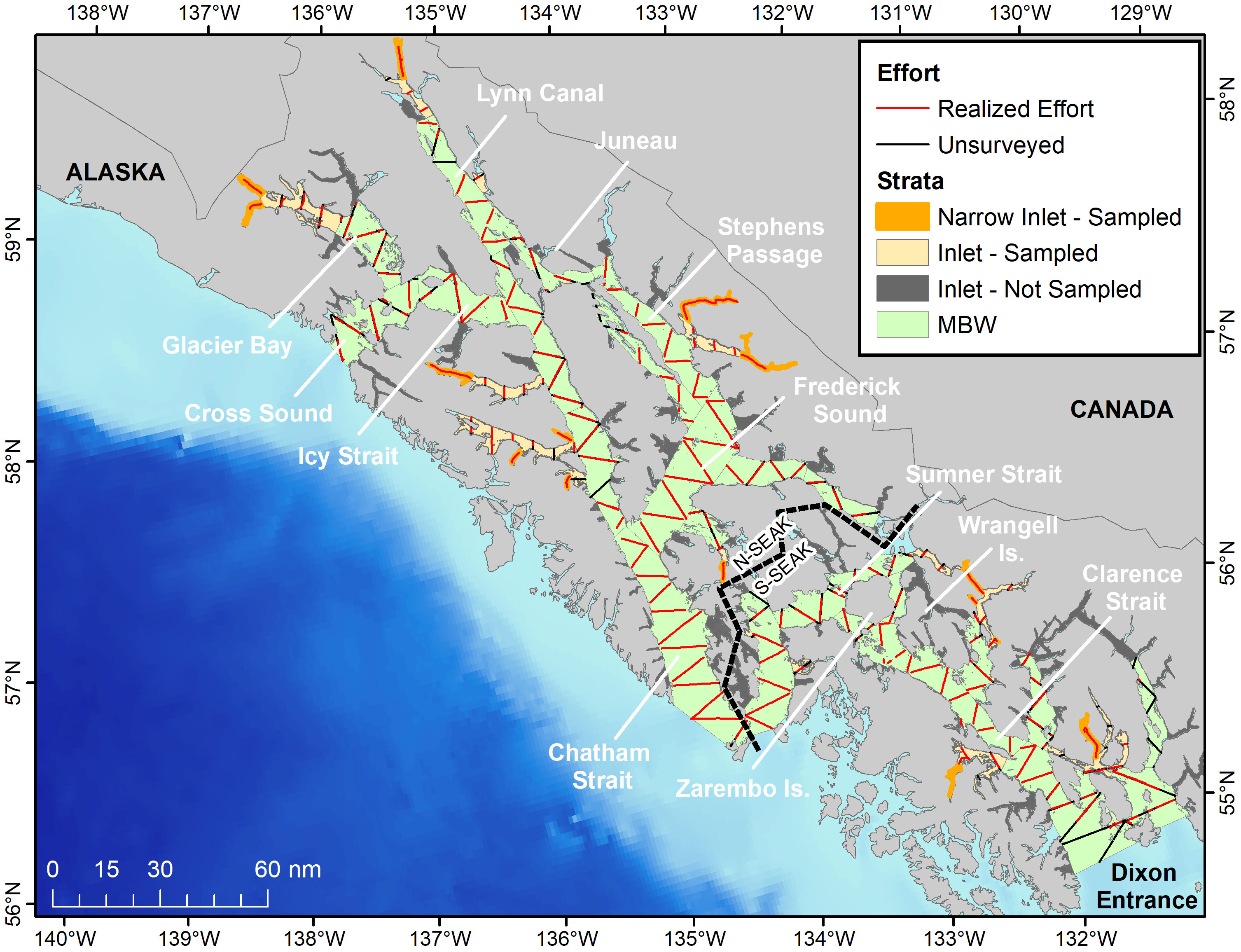
Figure 1 Realized survey effort (Beaufort 0-3) and unsurveyed sections of the proposed tracklines used to estimate abundance of harbor porpoise in SEAK in 2019.

The survey area was divided into two main strata of varying geometry (Figure 1): The stratum labeled “Main Water Bodies” (hereafter referred to as “MWB”) spanned an area of 18,632 km² (78.2% of the study area) and encompassed the main waterways of SEAK, including Cross Sound, Glacier Bay, Icy Strait, Chatham Strait, Frederick Sound, Stephens Passage, Summer Strait and Clarence Strait. The MWB largely coincided with areas sampled by previous harbor porpoise surveys in the region (Hobbs and Waite, 2010; Dahlheim et al., 2015). The stratum labeled “Inlets” (hereafter referred to as “I”) corresponded to an area of 5,189 km² (21.8% of the study area) and included small fjords, inlets and narrow straits and passages, the majority of which were not consistently surveyed in previous surveys.

Approximately 90% of the proposed effort (~2,700 km) was allocated to the MWB because it included the majority of the high concentration areas of harbor porpoise in the region (Dahlheim et al., 2015). To improve efficiency (e.g., minimize transit time between transects) and facilitate trackline allocation, the MWB stratum was divided into 26 sub-strata (Supplemental Material). The Inlet stratum was divided into 166 sub-strata (Figure 1), but it was not practical to sample all sub-strata because of their wide geographic distribution and complex geometric configuration. Therefore, the algorithm implemented by Thomas et al. (2007) for cluster sampling was used to select a sample of sub-strata to allocate the remaining 10% of effort. This algorithm had the following properties: (1) the probability of selecting sub-strata was proportional to its area size (e.g., larger areas had greater probability of selection), (2) the sample would have a wide geographic spread, and (3) and sub-strata would be sampled without replacement. Implementation of this algorithm resulted in a sub-sample of 13 sub-strata, corresponding to a total of 2,035 km² (or 39% of the area of the Inlets).

Survey lines were allocated proportional to the sub-stratum area using the design tool in the software Distance (version 7.2, Thomas et al., 2010). An equal spacing zig-zag design (Strindberg and Buckland, 2004) was adopted for the MWB whereas a parallel transect design was chosen for the Inlets given the narrowness of most areas (Strindberg and Buckland, 2004; Thomas et al., 2007). In extremely narrow sub-regions (e.g., 1-2 km wide) within Inlets, hereafter referred to as “narrow inlets”, it was more practical to search the whole area by surveying a line along the center of the inlet.

Field methods

The survey was carried out in passing mode (i.e., the ship did not divert from the trackline to close into detected cetacean groups, Hiby and Hammond, 1989; Hammond et al., 2021) using the R/V Zephyr, a 24m research vessel. Two types of survey lines were sampled: “Tracklines” and “Transit lines”. The former corresponded to survey lines laid out according to the design described above and the latter corresponded to lines connecting tracklines or transiting between different survey regions. The sampling protocol described below was used to collect sighting information on both types of lines.

Four observers rotated through two observation platforms (port and starboard) located 4m above the water level (mean eye height of 5.7m) every 40 minutes (each observer alternating between 80 minutes on-effort and 80 minutes resting). Observations started approximately 30 minutes after sunrise, ended 30 minutes before sunset, and were suspended in poor visibility conditions and/or sea state above 4 on the Beaufort scale. Port and starboard observers searched for cetaceans from the beam (90°) of their respective side to approximately 10° on the opposite side of the survey line using Fujinon 7x50 reticle binoculars (~80% of the time) or naked eye (~20% of the time). Two additional scientists rotated (every 2 hours) as data recorders. Recorders were not involved in active searching, but assisted observers with species identification and/or group size estimates when necessary. Occasionally, porpoise groups were first detected by the data recorder or a crew member, but these were not logged until reported by the observers or after the sighting passed abeam and had clearly been missed by the observer.

Data were entered into a laptop computer connected to a portable GPS using the program WinCruz (R. Holland, NOAA Southwest Fisheries Science Center). Position information was automatically logged every two minutes; navigational and environmental information was entered at the start of the day, at every observer rotation, and when conditions changed; and sighting information was recorded whenever marine mammals were detected. Weather and visibility conditions change frequently in SEAK with the potential to influence the observer search pattern. To maximize data collection, observers maintained search effort under light rain and also under foggy conditions when the visibility was greater than ~2km. However, the search protocol changed slightly under these two conditions: when light rain was present, less time was spent looking through binoculars due to wet lenses; and when fog was present, distance had to be visually estimated because a reference point (horizon or land) was no longer available as a baseline for binocular reticles. Search effort ceased in moderate to severe rain or if visibility in foggy conditions was less than ~2 km.

Analytical methods

Radial and perpendicular distance calculation

Radial distances were computed as described in Dahlheim et al. (2015). The distance from the vessel to each porpoise group was computed from reticle readings in the binoculars, assuming the reticles were placed at the horizon. However, in inland waters of SEAK, groups are often seen against land (as opposed to the “true horizon”). In these cases, the shoreline was used as the “horizon”, requiring distances to be re-computed. All group detections were plotted in GIS software and a line representing the distance to the real horizon, at the correct radial angle, was drawn. The horizon line was truncated wherever it crossed land. The length of this new line, representing the distance from the observer to the shore at the angle of the sighting, was then converted to “reticles to land” using the formulas described in Lerczak and Hobbs (1998), to account for the corresponding observer height and radians per reticle for 7×50 binoculars. Final distance from the observer to the group was calculated from this new reticle value with the DistRet function in the Excel add-in geofunc. Perpendicular distances were computed by multiplying the radial distance by the sine of the radial angle.

Density and abundance

Density and abundance were computed using a combination of line- and strip-transect methods. Estimates were obtained separately for N-SEAK and S-SEAK DIPs, which are separated by a boundary located east of Chatham Strait and south of Frederik Sound (Figure 1). Initially, density that was uncorrected for animals missed on the trackline was estimated in each stratum and each DIP separately, assuming a common detection function. Only tracklines sampled in relatively low sea-state conditions (Beaufort 0-3) were considered in density estimation. Data collected on transit lines were only used to estimate detection probability.

For the MWB stratum, density in the area covered by the tracklines was estimated using the Horvitz-Thompson (HT) estimator as described in Marques and Buckland (2003) and implemented in package mrds (Laake et al., 2021) in the open-source software R 4.2.1 (R Core Team, 2021). Abundance was computed by multiplying density by the total area of the MWB stratum assumed to correspond to each stock.

For the Inlet stratum, a combination of line- and strip-transect methods was used in the estimation of density. In the “wider” inlets the same line transect procedures described for the MWB above were applied. In contrast, no detection probability was estimated for the narrow inlets and density was simply computed as the number of individuals seen within the sampling strip divided by the area of the inlet (e.g., a strip transect approach). Overall density in the Inlet stratum was calculated as the average of the estimated density in the wide and narrow inlets weighted by the area surveyed in each inlet type. Overall density was then extrapolated to the area of the I stratum in each DIP (166 identified inlets) to estimate abundance.

Overall abundance of the northern and southern DIPs was computed by summing the abundance from the MWB and I strata in each region, respectively. The mathematical formulation of the analytical methods used to estimate density and abundance in this study is described in the Supplemental Material.

Effective strip width (ESW)

Conventional (CDS) and Multiple Covariate Distance Sampling (MCDS) methods (Buckland et al., 2001; Marques and Buckland, 2003) were used to estimate detection probability (P) by modeling unbinned perpendicular distance data truncated at 1.5 km, using porpoise groups detected by the observer team on tracklines and transit lines. A half-normal model without adjustments, but with covariates, was proposed because it exhibits greater stability in fitting cetacean sighting data when compared to other commonly used models (e.g., the hazard rate) (Gerrodette and Forcada, 2005; Bradford et al., 2020). Covariates used to model P included group size (as a discrete covariate), sea state (a categorical variable with two states, “low” [Beaufort 0-2] and “high” [Beaufort 3], Dahlheim et al., 2015) and observer (also categorical with 5 levels). A categorical “visibility” covariate, with three levels, was also included to accommodate potential differences in search patterns when search mode changed to “wet” or “foggy” conditions. A total of 16 models were proposed and covariates were tested both individually and additively. A single harbor porpoise sighting detected by the crew, but not seen by the observers was excluded from the analysis before fitting the perpendicular distance data. The effective strip half width (ESW) was computed by multiplying P by the truncation distance (1.5km). In the narrow inlets, it was assumed that all animals at the surface were detected (P=1) because shore was within 500-1000m form the ship and therefore visible on both sides of the survey line.

Group size estimation

If larger groups are easier to detect further away from the trackline than smaller groups, using average group size can bias estimates of density and abundance (Buckland et al., 2001). Therefore, exploratory analysis were conducted to evaluate this potential source of bias. Detections as a function of distance were determined to be independent of group size, so mean group size was used in estimating density and abundance for CDS models. For MCDS models, estimates of expected group size were obtained by dividing the estimated density of individuals by density of groups (Marques and Buckland, 2003) (see also Supplemental Material).

Estimation of trackline detection probability (g[0])

Line transect surveys typically assume perfect detection probability on the trackline (i.e. g(0) = 1) (Buckland et al., 2001), but this assumption is rarely true for cetacean surveys, particularly for harbor porpoise (Palka, 1995; Laake et al., 1997; Laake and Borchers, 2004). Animals are often missed because they are submerged (availability bias) or because they are not seen by observers even when they are available due to factors such as weather and sea conditions (perception bias) (Marsh and Sinclair, 1989). In shipboard surveys, g(0) is often estimated using double platform methods (Palka, 1995; Hammond et al., 2013), but it was not possible to implement this method in this survey due to logistical constraints. Instead, we used an approach analogous to the method presented by Barlow (2015) that computes g(0) from apparent density in different sea states. This approach assumes that true density does not change with sighting conditions, but rather that detectability on the trackline decreases as survey conditions deteriorate.

Survey data from line-transect cruises conducted in 1991-93, 2006-7 and 2010-2012 (Dahlheim et al., 2015) were used to compute estimates of g(0). Those surveys were conducted using methods analogous to those implemented in the present study. Only data from Glacier Bay and Icy Strait (Region 1 in Dahlheim et al., 2015) were used because estimated abundance was believed to be stable in these locations across survey periods (Dahlheim et al., 2015). A total of 1,066 porpoise groups (275, 512, 210 and 69 groups observed in, respectively, Beaufort 0, 1, 2 and 3) recorded in Glacier Bay and Icy Strait were available to compute estimates of g(0). Following the methods stated above, sea-state category (“low” and “high”) and year were used as covariates to fit perpendicular distance data. These two variables were chosen because they were determined to influence detection probability during the SEAK line-transect surveys reported in Dahlheim et al. (2015). Group density was estimated for Beaufort states 0 to 3 separately and a Beaufort-specific (relative) g(0) was computed as the ratio between density in a given state and density in Beaufort 0, for which g(0) was assumed perfect (Barlow, 2015; Supplemental Material). Overall g(0) was computed as the average of the Beaufort category-specific relative g(0) weighted by the effort in that category in the 2019 survey (Bradford et al., 2020) and applied to uncorrected estimates of density and abundance for the present survey.

Estimation of uncertainty

Uncertainty of model parameters and other variables was estimated using a non-parametric bootstrap approach. For each of 1,000 bootstrap replicates, survey tracklines within each stratum were re-sampled with replacement. Detection probability was estimated from porpoise groups detected on these lines. Model uncertainty in detection probability estimation was incorporated by fitting all proposed detection probability models to perpendicular distance in each bootstrap replicate. Models were then ranked by their Akaike Information Criterion (AIC) and the model with most support (lowest AIC) was selected to compute abundance for that replicate. Constraints were imposed to avoid the use of erroneous models in fitting the detection function. For example, models that did not conform to their expectation (e.g., a model that suggested a positive correlation between P and Beaufort state, or a negative correlation between P and group size) were removed from the set of candidate models prior to ranking. Encounter rate, group size, density, and abundance were computed for each stratum in each region as specified above. Standard errors were computed as the standard deviation of the distribution of bootstrap replicates and 95% confidence intervals were estimated as the 2.5^th and the 97.5^th quantile of this same distribution.

Bootstrap methods were also used to compute variance in estimates of g(0). For each bootstrap replicate, survey lines from the 1991-93, 2006-7 and 2010-12 data in Dahlheim et al. (2015) were re-sampled with replacement, detection probability was estimated as described above and relative g(0) values were computed from Beaufort-specific density estimates. An average g(0) for that replicate was calculated from these relative g(0) values, weighted by effort in each Beaufort sea state surveyed in 2019.

N_min and PBR level calculation

The Potential Biological Removal (PBR, Wade, 1998) level is defined under the MMPA as the maximum number of animals that may be removed from a marine mammal stock (excluding natural mortality) while allowing the stock to maintain its optimum sustainable population (defined to be a range between maximum productivity and carrying capacity, Wade, 1998). The derivation of PBR is defined within the MMPA, and the specific details of how to calculate PBR were defined in subsequent publications and U.S. federal regulations (e.g., Barlow et al., 1995; Federal Register 81 FR 1083, 2 March 2016), based on simulations to that determined the thresholds that would allow 95% of populations to be at or above their Optimum Sustainable Population (OSP) level after 100 years (Wade (1998). For each marine mammal stock, PBR is thus computed as a single value: PBR = N_min * 0.5R_max * F_R, where N_min corresponds to the 20th percentile of the abundance estimate, R_max is a measured or estimated maximum net population growth rate (or a taxon-specific conservative default value), and the recovery factor (F_R) is a single value, set based on the level of uncertainty in human-caused mortality estimates and the population’s status.

The N-SEAK DIP and S-SEAK DIP are under consideration for being designated separate stocks under the MMPA. Therefore, we have calculated tentative PBR levels for each of these DIPs using the abundance estimates derived in this study. The growth rate R_max is unknown for harbor porpoise in Southeast Alaska, so the default value for cetaceans (R_max = 0.04) was applied. F_R was 0.5, as specified for stocks of unknown status. We included these tentative PBR calculations to assess whether the known impacts of some anthropogenic activities should be highlighted as a possible conservation concern. However, as part of the process under the MMPA, the boundaries of the DIPs, and the calculations of N_min and PBR levels are subject to public review and comment and may be revised as a result of that input.

Results

A total of 2,893 km (312 survey lines) was surveyed in sea-state conditions ranging from Beaufort 0 to 3 during the 2019 survey. Trackline effort corresponded to 1,120 km (102 sampling lines) and 482 km (62 sampling lines) within the range of the N-SEAK and S-SEAK DIPs, respectively, whereas transit effort consisted of 1,291 km (148 sampling lines) across both regions (Table 1). A total of 194 on-effort harbor porpoise groups comprising 301 individuals was documented (Table 1). Completed effort in each region is illustrated in Figure 1.

TABLE 1

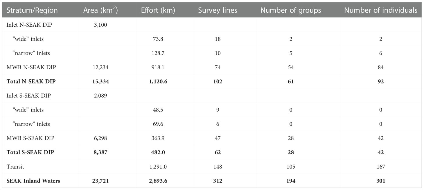
Table 1 Sampled area, survey effort and number of groups and individuals seen during the 2019 harbor porpoise survey in Southeast Alaska inland waters. Rows in bold represent totals across the N-SEAK DIP, the S_SEAK DIP and the whole of SEAK Inland Waters.

Harbor porpoise distribution

The distribution of harbor porpoise in SEAK inland waters during the summer 2019 cruise is illustrated in Figure 2. High concentrations of animals were seen near Glacier Bay, Icy Strait, Cross Sound, Frederick Sound, and in Sumner Strait and around Wrangell and Zarembo Islands. Occasional porpoise groups were recorded in other regions including Lynn Canal, Stephens Passage, Chatham Strait, and Clarence Strait. Harbor porpoises were also occasionally seen in the sampled inlets, but only within the range of the N-SEAK DIP.

FIGURE 2

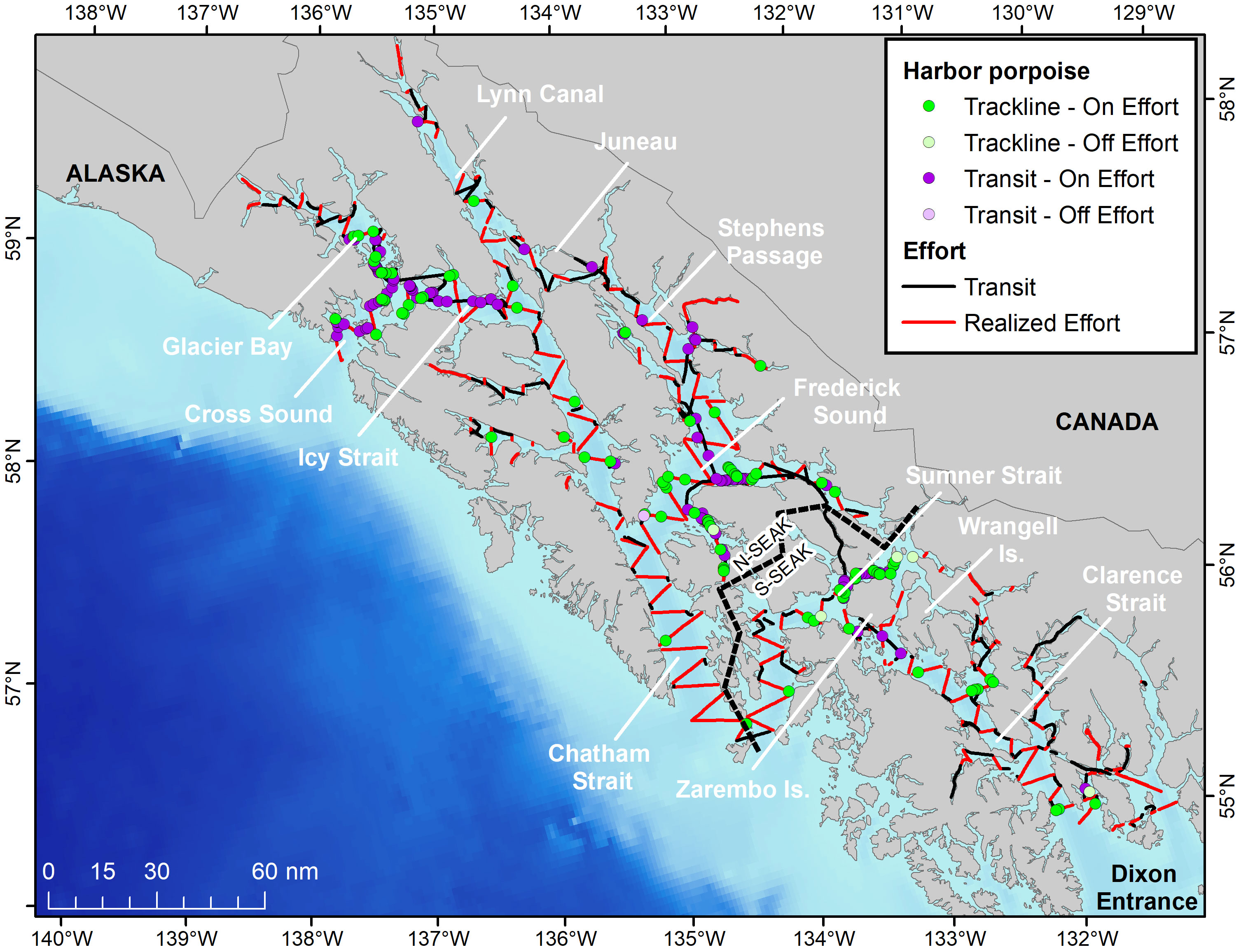
Figure 2 Harbor porpoise distribution during the 2019 SEAK survey. Porpoise groups detected on- and off-effort are indicated by darker and lighter green circles and realized effort is shown as red lines.

Effective strip width and g(0)

Detection probability (P) and ESW were estimated as 0.48 (CV = 0.09, 95% CI = 0.40-0.58) and 726 m (CV = 0.09, 95% CI = 603-856 m), respectively. The proposed covariates were important in fitting the detection probability models. Models with none, one, two, three and all four covariates represented, respectively, 4.2%, 23.5%, 40.1%, 29.6% and 2.6% of the most supported models in the 1,000 bootstrap replicates. The “observer” covariate was present in 87.7% of the models, indicating that detection probability was significantly different across observers. The “visibility” and “Beaufort Category” covariates were present in 69% and 50% of the models, respectively, showing that lower visibility (e.g., fog and wet effort) and poorer sea conditions (“high” Beaufort) negatively affected detection probability. Finally, the group size covariate was present in only 4.2% of the most supported models, indicating that group size did not influence the probability of detecting harbor porpoise as much as the other covariates within SEAK inland waters. An example of a detection probability model fit to perpendicular distance data from one of the bootstrap replicates is provided in the Supplemental Material.

Detection probability on the trackline, g(0), was estimated as 0.53 (CV = 0.11, 95% CI = 0.43-0.65). A summary of the Beaufort-specific, relative g(0) values, and the proportions of effort in each Beaufort state used in the computation of g(0) is provided in the Supplemental Material.

Density and abundance

Harbor porpoise abundance was estimated as 1,619 (CV = 0.26, 95% CI = 944-2,592) for the N-SEAK DIP, and 890 (CV = 0.37, 95% CI = 385-1,708) for the S-SEAK DIP. Estimates of encounter rate, expected group size, density (corrected for g[0]), and abundance (corrected for g[0]) are provided in Table 2. Summaries of the bootstrap estimates for region/stratum-specific parameters and other quantities of interest are provided in the Supplemental Material.

TABLE 2

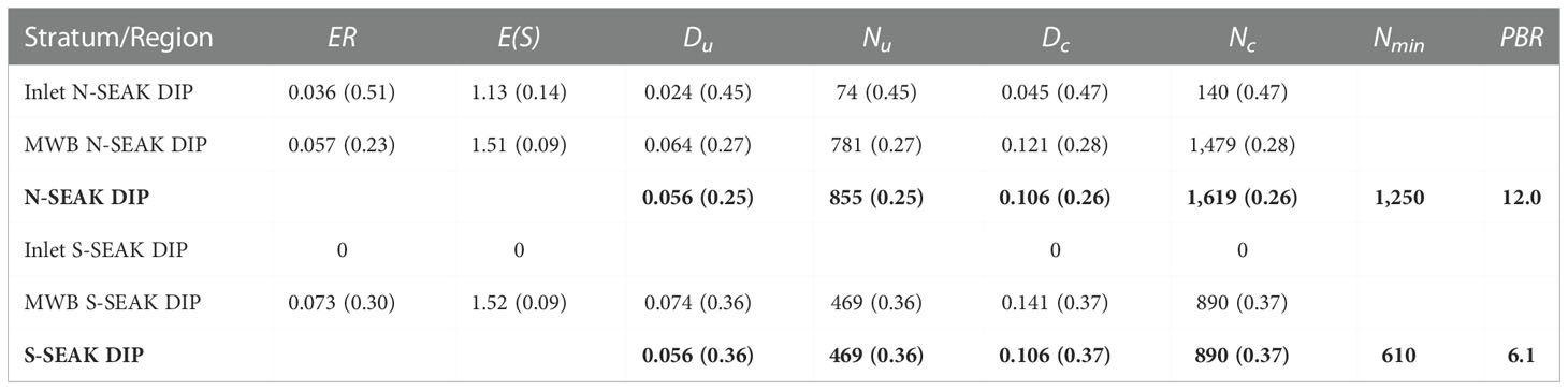
Table 2 Estimates (CV in parenthesis) of encounter rate (ER, groups/km), expected groups size (E[S], individuals), uncorrected and corrected density (D_u and D_c, individuals/km2), uncorrected and corrected abundance (N_u and N_c, individuals), minimum population size (N_min) and the Potential of Biological Removal (PBR) for harbor porpoise in SEAK inland waters. Rows in bold represent total estimates for the N-SEAK DIP and the S-SEAK DIP.

For the N-SEAK DIP, density of harbor porpoise was lower in the Inlets than in the MWB stratum. Slightly less than 10% of the population estimated for the N-SEAK DIP occurred in the Inlets. No harbor porpoise were observed in the Inlets in the southern region and, therefore, no abundance was computed for that stratum. Region-specific density (0.106 ind/km²) was identical for the N-SEAK and S-SEAK DIPs, but abundance in the former was nearly twice that of the southern DIP because of its larger area.

N_min and PBR calculation

Estimates of N_min and PBR for N- and S-SEAK DIPs are provided in Table 2. PBR was estimated at 12.0 and 6.1 animals for these populations, respectively.

Discussion

Survey design

SEAK is a difficult region to survey due to its complex geography, which includes a network of open but relatively convoluted channels and narrow straits and inlets. Previous surveys to estimate cetacean abundance in this region (Hobbs and Waite, 2010; Dahlheim et al., 2015) did not fully consider geographical heterogeneity in their sampling design and the resulting estimates may have been biased. For example, sampling of small inlets, where the harbor porpoise is known to occur (J. Straley, pers. comm.), has seldom occurred and, when it did, sampling was not performed in a systematic fashion. In addition, even in areas where sampling was performed more regularly, tracklines were not allocated to achieve near uniform coverage probability.

In the present study, we applied more rigorous methods for conducting cetacean line-transect surveys to compute abundance in complex regions (Thomas et al., 2007). Additionally, the survey design implemented in this study allowed the sampling of all possible harbor porpoise habitats within SEAK, including narrow channels and inlets, which were previously unsurveyed. In this design, tracklines were allocated to achieve near uniform coverage probability across the different strata. Unusually good visibility conditions (Beaufort 3 or less for 92% of the survey) allowed for completion of the planned tracklines in most regions, particularly those where harbor porpoises are known to occur (see Figure 2). Exceptions include areas closer to open ocean (e.g., the southern end of Clarence Strait, near Dixon Entrance) and middle Lynn Canal. But even in these regions, loss of trackline effort was limited and broad sampling was achieved. The relatively extensive and uniform coverage of porpoise habitats within SEAK inland waters during the 2019 survey resulted in more comprehensive sampling and potentially more accurate estimates of abundance than those obtained from previous harbor porpoise surveys in SEAK.

Harbor porpoise distribution

In some areas of SEAK, harbor porpoise have been consistently found in relatively high numbers across years. For example, harbor porpoise concentrations observed during our survey are consistent with those found between the early 1990s and early 2010s near Cross Sound, Glacier Bay, Icy Strait and around Zarembo and Wrangell Islands in the spring, summer and fall (Dahlheim et al., 2009; Dahlheim et al., 2015). On the other hand, in Frederick Sound the concentration of harbor porpoise is variable across years. During the 2019 cruise, porpoises were seen in Frederick Sound in relatively large numbers, especially close to shore (Figure 2). However, in some previous years, concentration was low despite high survey effort (e.g., Dahlheim et al., 2015).

Another region of interest is Lynn Canal, where harbor porpoise were regularly documented in the 1990s (Hobbs and Waite, 2010; Dahlheim et al., 2015). Surveys did not sample this region in the mid-2000s and early 2010s; a relatively small number of groups were observed in 2019 (Figure 2). This area is of particular interest because the salmon drift net fishery, in which harbor porpoise bycatch has been documented in other regions, operates there (Manly, 2015). However, no recent monitoring of the fishery to assess potential bycatch levels has been conducted.

Results from this study found that harbor porpoise do not regularly occur in certain habitats within SEAK. For example, in Lower Chatham Strait, only one harbor porpoise sighting was recorded despite the relatively consistent survey effort in this region (and in good survey conditions) (Figure 2). Despite significant survey effort across many years, Dahlheim et al. (2009); Dahlheim et al., 2015) and Hobbs and Waite (2010), also reported few harbor porpoise in Lower Chatham Strait although observation effort in Dahlheim et al. (2015) was typically associated with poorer survey conditions (e.g., relatively high sea state conditions).

In this survey, SEAK inlets were sampled consistently for the first time and abundance was computed using a proven method (e.g., Thomas et al., 2007). Estimation of density in narrow (<2km width) inlets assumed that observers detected all harbor porpoise because they were able to see both shores while surveying these inlets. If this assumption is not valid, then estimates in the inlet stratum would be underestimated. Nevertheless, bias of the overall abundance estimation is believed to be nearly negligible, if it occurred, because of the low number of harbor porpoise observed and the relatively small area of the narrow inlets compared to the other survey strata.

Previous surveys of harbor porpoise in inland waters of SEAK only sampled inlets occasionally and no estimates of abundance were computed. The results provided here suggest that while harbor porpoises regularly occur in the inlets, they represent a small fraction of the overall population (e.g., approximately 10% of the northern DIP). No porpoise groups were recorded in inlets in the southern DIP during the 2019 survey. However, this finding does not imply harbor porpoises do not visit inlets it that region. This species has been occasionally observed in southern DIP inlets during previous surveys (Hobbs and Waite, 2010; Dahlheim et al., 2015).

Density, abundance estimation, and PBR

This study provides new density and abundance estimates for harbor porpoise in inland waters of SEAK, including areas where harbor porpoise are genetically differentiated (N-and S-SEAK DIPs) (Parsons et al., 2018; Parsons et al., 2021). These estimates incorporate detection probability on the trackline (g[0]) an important aspect of calculating abundance for SEAK harbor porpoise. Apart from the aerial survey by Hobbs and Waite (2010) in the late 1990s, previous estimates of abundance were not corrected for animals missed on the trackline (Dahlheim et al., 2000; Dahlheim et al., 2015). For inconspicuous species such as harbor porpoise, deterioration of optimal visibility conditions result in observers missing groups (Barlow, 2015). Therefore, correction for g(0) is required to minimize negative bias in estimates of abundance of this species (Barlow, 1988; Palka, 1995; Polacheck, 1995; Hammond et al., 2013). Estimation of g(0) in harbor porpoise studies has typically been based on surveys where observers scan for porpoise groups from two independent platforms. Analytical methods combining distance-sampling and mark-recapture approaches are used to estimate the proportion of animals missed by these observers on the trackline (Laake and Borchers, 2004). In this study, logistical constraints precluded the implementation of independent platforms and required an alternate method to estimate g(0). The approach used here was analogous to that developed by Barlow (2015) to compute trackline detection probability from densities in different survey conditions. This method assumes that true density does not change with sighting conditions and that estimated density under optimal conditions will be less biased than density estimates in poorer conditions. In this study, harbor porpoise groups detected in previous surveys in SEAK (from the 1990s to the early 2010s) were used to estimate density for different visibility conditions (denoted by the Beaufort scale) because this provided an independent data set with substantially larger sample sizes. Data from only one region in SEAK (the area around Glacier Bay and Icy Strait, region 1 in Dahlheim et al., 2015) were used because that is an important harbor porpoise habitat and because density estimates in that region have remained stable during the study period (Dahlheim et al., 2015). While data from a broader area (e.g., the whole of SEAK) could be used, Barlow (2015) suggested that differences in densities due to habitat preference or due to temporal trends in abundance could bias estimates of g(0). Therefore, the use of the Glacier Bay and Icy Strait data minimized these potential undesired effects.

The estimated g(0) value computed here, based on a weighted-average over sea-state conditions, (g[0] = 0.53, CV = 0.11, 95% CI = 0.43-0.65) implies that overall, approximately 47% of the harbor porpoise groups on the trackline are missed. This estimate falls within the range of estimates obtained across several other harbor porpoise ship-board surveys. For example, Barlow (1988) estimate of g(0) for the coast of California harbor porpoise (g[0] = 0.78, CV = 0.15, 95% CI = 0.45-0.95) and Palka (1995) area-weighted average of g(0) for harbor porpoise in the Gulf of Maine (g[0] = 0.72, CV = 0.08, 95% CI = 0.60-0.84¹) are higher than the one computed for SEAK, but they were both estimated for larger survey platforms and are likely not statistically different. In contrast, the estimated g(0) for harbor porpoise in continental shelf waters of the European Atlantic Ocean (Hammond et al., 2013; g[0] = 0.22, CV = 0.16, 95% CI = 0.15-0.28¹) is significantly lower than for SEAK. The direct comparison of g(0) estimates across surveys is difficult because of differences in vessel size, number of observers, search methods, and survey conditions.

The use of a g(0) estimated with data from previous SEAK harbor porpoise surveys to correct density estimates from the 2019 cruise is only valid if the sampling methods across the surveys are comparable. The vessels used by Dahlheim et al. (2015) were slightly larger than the one used in this study and observers were different. However, the number of observers on effort, search patterns, and survey conditions were largely similar. Differences in observers are particularly relevant because, as shown in this study, detection probability can be significantly influenced by observer experience and their individual ability to detect porpoise. If the g(0) computed from data in Dahlheim et al. (2015) is not applicable to the 2019 SEAK harbor porpoise survey, the estimates of density and abundance corrected for g(0) provided here will be biased to an unknown extent. The approach to compute g(0) used in this study was applied to address an important source of bias in harbor porpoise surveys. However, as stated in Barlow (2015), this method is “intended to complement rather than replace more traditional methods of estimating g(0), and every effort should be made to incorporate g(0) estimation into the design of any cetacean survey”. Because survey logistics, protocols and conditions vary, future studies in SEAK should consider the use of methods (e.g., double observer platform surveys) that would allow estimation of g(0) for each new survey.

The estimated average ESW in this study (726 m) was comparable to those from previous surveys in Southeast Alaska, which ranged from 705 to 915 m (Dahlheim et al., 2015). This is to be expected because similar field methods were used across these surveys. However, these values are substantially greater than ESW computed for harbor porpoise in other regions. Harbor porpoise surveys in the Gulf of Maine/Bay of Fundy (Palka, 1995; Palka, 2000), the west coast of North America (Barlow, 1988; Williams and Thomas, 2007), and in European waters (Bjørge and Donovan, 1995; Hammond et al., 2013) estimated ESW values ranging from approximately 130 and 375 m. While various factors influence estimation of detection probability (e.g., height of the vessel, number of observers, porpoise searching methods), most of these open ocean surveys were conducted using similar searching methods (e.g., 7x50 binoculars and/or naked eye), from higher platforms and with an equal or larger number of observers when compared to surveys in SEAK inland waters. Therefore, it would be expected that ESW estimated in these surveys to be comparable or potentially even greater than those computed for SEAK inland waters. Greater ESW for harbor porpoise in SEAK likely occurs because survey conditions in inland waters improve visibility of this species. For example, the presence of land in most of the region allows observers to focus on a smaller search area ahead of the vessel, possibly increasing their detectability. Perhaps more importantly, sea conditions are typically more favorable in inland waters and large swells, which greatly affect detection of cetaceans at sea (Barlow et al., 2001), were uncommon within most of SEAK inland waters where harbor porpoise were documented in the 2019 survey.

Abundance estimates provided here do not include animals found outside of SEAK inland waters. Aerial surveys have shown that harbor porpoise occur on the continental shelf west of the SEAK inland waters (Dahlheim et al., 2000; Hobbs and Waite, 2010), but no recent estimate for offshore habitats are available. In addition, it is unclear what the phylogenetic relationship is between harbor porpoise found offshore and those in the N-SEAK and S-SEAK DIPs. It is possible that these DIPs extend into open ocean waters of the Gulf of Alaska, west of SEAK inland waters but further research is needed to assess the population structure of harbor porpoise in this region. The abundance and density estimates computed in this study correspond to the currently defined DIPs in inland waters.

A potentially important conservation problem for harbor porpoises is bycatch in the salmon drift gillnet fishery, which operates in parts of the SEAK inland waters, notably Lynn Canal, Taku/Snettisham and Stephens Passage, near Petersburg, Wrangell, Zarembo, Ketchikan, and in portions of Clarence Strait (Manly, 2015). There is no current estimate of bycatch for all regions where the fishery operates. In 2012 and 2013, the Alaska Marine Mammal Observer Program (AMMOP) established a monitoring program to observe the gillnet fishery in the Alaska Department of Fish and Game’s (ADF&G) fisheries districts 6, 7 and 8 in order to estimate bycatch and serious injuries of marine mammals and birds. Areas 6, 7 and a portion of area 8 correspond to a relatively large portion of the S-SEAK DIP range, near Wrangell and Zarembo, where harbor porpoise density is relatively high (Dahlheim et al., 2015; this study). A smaller portion of Area 8, the eastern end of Frederik Sound, corresponds to the southern range of the N-SEAK DIP. AMMOP observed 6.4% and 6.6% of the fishing days in each in 2012 and 2013, respectively, and recorded the capture of four harbor porpoise in 2013, with two being released alive and two being classified as dead or seriously injured (M/SI) (Manly, 2015). Manly (2015) estimated 23 harbor porpoise M/SI from observer data in ADF&G Districts 6, 7 and 8 for the period 2012-2013 (an average of 12 individuals per year). An error was identified in the way the injury determinations were assigned to two of the bycaught animals in Manly (2015) (Zerbini et al., 2022). Two individuals caught in sub-area 8A were reported to be serious injuries (Manly, 2015), but upon review of the data, it was confirmed that one of these individuals should have been classified as having a non-serious injury, as documented in Helker et al. (2015). On the other hand, the porpoise captured in sub-area 6A and classified as a non-serious injury in Manly (2015) was in fact a seriously injured animal (Helker et al., 2015). A revised estimate suggests that bycatch mortality in the range of the N-SEAK and S-SEAK DIPs correspond to, respectively, 5.6 and 7.4 harbor porpoises per year (Young et al., 2022). These estimates suggest a potential conservation problem for the S-SEAK DIP as mortality is above the tentative estimated PBR level (6.1 individuals) for this population. The status of harbor porpoise in the N-SEAK DIP is unknown because existing estimates of mortality only apply to a portion of the fishery operating in the range of this population. However, the tentative estimated PBR level (12 individuals) would suggest that harbor porpoise in the northern region may not sustain a much higher mortality/serious injury rate than that estimated for the portion of the fishery that has already been observed. Changes to the boundaries of the DIPs and the calculation of the N_min and PBR level may occur as a result of the public review and comment period and could affect our interpretation of the impact of the bycatch on harbor porpoise in SEAK.

Several studies have shown that harbor porpoise are highly vulnerable to mortality in gillnet fisheries across the range of the species (Read et al., 1993; Trippel et al., 1996; Tregenza et al., 1997; Reeves et al., 2013) and declines in abundance have been documented for some populations (Forney et al., 2021; Nachtsheim et al., 2021). Therefore, monitoring abundance and bycatch of harbor porpoise is critical to evaluate the potential impact of the gillnet fishery to this species in SEAK and to assess the need to implement mitigation measures to reduce mortality.

Data availability statement

The raw data supporting the conclusions of this article will be made available by the authors, without undue reservation.

Ethics statement

The animal study was reviewed and approved by Alaska Fisheries Science Center/Northwest Fisheries Science Center Animal Care and Use Committee.

Author contributions

AZ and KG designed the study. All authors collected the data. AZ and KG analyzed the data. AZ wrote the initial manuscript draft. All authors contributed to the article and approved the submitted version.

Funding

Funding for this research was provided by NOAA’s Office of Protected Resources and NOAA’s Alaska Regional Office.

Acknowledgments

The authors acknowledge the captain and crew of the R/V Zephyr for a safe and successful survey. Data collection was performed by a team of dedicated observers, which, in addition to the authors, included Chris Hoefer, Annie Masterman, and Adam Ü. We also thank Robyn Angliss, Phil Clapham, Nancy Friday, and Janice Waite for support for this research. The study was conducted under NMFS Permit 20465 issued to the Marine Mammal Laboratory, Alaska Fisheries Science Center, NOAA Fisheries.

Conflict of interest

The authors declare that the research was conducted in the absence of any commercial or financial relationships that could be construed as a potential conflict of interest.

Publisher’s note

All claims expressed in this article are solely those of the authors and do not necessarily represent those of their affiliated organizations, or those of the publisher, the editors and the reviewers. Any product that may be evaluated in this article, or claim that may be made by its manufacturer, is not guaranteed or endorsed by the publisher.

Author disclaimer

The views expressed here are those of the authors and do not necessarily reflect the views of the US National Marine Fisheries Service-NOAA Fisheries.

Supplementary material

The Supplementary Material for this article can be found online at: https://www.frontiersin.org/articles/10.3389/fmars.2022.966489/full#supplementary-material

Footnotes

1. ^ 95% CI computed assuming a normal distribution.

References

Angliss R., Wade P. R. (1997) Guidelines for assessing marine mammal stocks: report of the GAMMS workshop, April 3-5, 1996, Seattle, WA. Available at: www.nmfs.noaa.gov/pr/pdf/sars/gamms_report.pdf.

Google Scholar

Avila I. C., Kaschner K., Dormann C. F. (2018). Current global risks to marine mammals: Taking stock of the threats. Biol. Conserv. 221, 44–58. doi: 10.1016/j.biocon.2018.02.021

CrossRef Full Text | Google Scholar

Barlow J. (1988). Harbor porpoise, Phocoena phocoena, abundance estimation for California, Oregon and Washington: I. ship surveys. Fishery Bull. 86 (3), 417–432.

Google Scholar

Barlow J. (2015). Inferring trackline detection probabilities, g(0), for cetaceans from apparent densities in different survey conditions. Mar. Mammal Sci. 31 (3), 923–943. doi: 10.1111/mms.12205

CrossRef Full Text | Google Scholar

Barlow J., Gerrodette T., Forcada J. (2001). Factors affecting perpendicular sighting distances on shipboard line-transect surveys for cetaceans. J. Cetacean Res. Manage. 3 (2), 201–212.

Google Scholar

Barlow J., Swartz S. L., Eagle T. C., Wade P. R. (1995). U.S. marine mammal stock assessments: Guidelines for preparation, background, and a summary of the 1995 assessments. U.S. dep. commer., NOAA tech. memo. NMFS-OPR-6. 73.

Google Scholar

Birkun Jr A. A., Frantzis A. (2008) Phocoena phocoena ssp. relicta, black Sea harbor porpoise. the IUCN red list of threatened species 2008.T17030A6737111. Available at: http://dx.doi.org/10.2305/IUCN.UK.2008.RLTS.T17030A6737111.en.

Google Scholar

Bjørge A., Donovan G. P. (1995). Report of the international whaling commission (Special issue 16). biology of the phocoenids (Cambridge: International Whaling Commission), 552.

Google Scholar

Bradford A. L., Becker E. A., Oleson E., Forney K. A., Moore J. E., Barlow J. (2020). Abundance estimates of false killer whales in Hawaiian waters and the broader central pacific (Hawaii: National Marine Fisheries Service), 78.

Google Scholar

Braulik G., Minton G., Amano M., Bjørge A. (2020). Phocoena phocoena. The IUCN Red List of Threatened Species 2020: e.T17027A50369903. doi: 10.2305/IUCN.UK.2020- 2.RLTS.T17027A50369903.en.

Google Scholar

Buckland S. T., Anderson D. R., Burnham K. P., Laake J. L., Borchers D. L., Thomas L. (2001). Introduction to distance sampling: Estimating abundance of biological populations (New York, United States: Oxford University Press), 432.

Google Scholar

Carlén I., Nunny L., Simmonds M. P. (2021). Out of sight, out of mind: How conservation is failing European porpoises. Front. Mar. Sci. 8. doi: 10.3389/fmars.2021.617478

CrossRef Full Text | Google Scholar

Carretta J. V., Forney K. A., Oleson E. M., Weller D. W., Lang A. R., Baker J., et al. (2019). U.S. pacific marine mammal stock assessments: 2018 Vol. 617 (U.S. Department of Commerce), 382. doi: 10.25923/x17q-2p43

CrossRef Full Text | Google Scholar

Dahlheim M. E., White P. A., Waite J. M. (2009). Cetaceans of southeast Alaska: distribution and seasonal occurrence. J. Biogeogr. 36 (3), 410–426. doi: 10.1111/j.1365-2699.2008.02007.x

CrossRef Full Text | Google Scholar

Dahlheim M., York A., Towell R., Waite J., Breiwick J. (2000). Harbor porpoise (Phocoena phocoena) abundance in Alaska: Bristol bay to southeast alaska 1991-1993. Mar. Mammal Sci. 16 (1), 28–45. doi: 10.1111/j.1748-7692.2000.tb00902.x

CrossRef Full Text | Google Scholar

Dahlheim M. E., Zerbini A. N., Waite J. M., Kennedy A. S. (2015). Temporal changes in abundance of harbor porpose (Phocoena phocoena) inhabiting the inland waters of southeast Alaska. Fishery Bull. 113 (3), 242–255. doi: 10.7755/FB.113.3.2

CrossRef Full Text | Google Scholar

Forney K. A., Moore J. E., Barlow J., Carretta J. V., Benson S. R. (2021). A multidecadal Bayesian trend analysis of harbor porpoise (Phocoena phocoena) populations off California relative to past fishery bycatch. Mar. Mamm. Sci. 37, 546–560. doi: 10.1111/mms.12764

CrossRef Full Text | Google Scholar

Gerrodette T., Forcada J. (2005). Non-recovery of two spotted and spinner dolphin populations in the eastern tropical pacific ocean. Mar. Ecol. Prog. Ser. 291, 1–21. doi: 10.3354/meps291001

CrossRef Full Text | Google Scholar

Hammond P. S., Bearzi G., Bjørge A., Forney K. A., Karczmarski L., Kasuya T., et al. (2008) Phocoena phocoena (Baltic Sea subpopulation). the IUCN red list of threatened species 2008: e.T17031A98831650. Available at: http://dx.doi.org/10.2305/IUCN.UK.2008.RLTS.T17031A6739565.en.

Google Scholar

Hammond P. S., Francis T. B., Heinemann D., Long K. J., Moore J. E., Punt A. E., et al. (2021). Estimating the abundance of marine mammal populations. Front. Mar. Sci. 8 (1316). doi: 10.3389/fmars.2021.735770

CrossRef Full Text | Google Scholar

Hammond P. S., Macleod K., Berggren P., Borchers D. L., Burt M. L., Cañadas A., et al. (2013). Distribution and abundance of harbour porpoise and other cetaceans in European Atlantic shelf waters: implications for conservation and management. Biol. Conserv. 164, 107–122. doi: 10.1016/j.biocon.2013.04.010

CrossRef Full Text | Google Scholar

Helker V. T., Allen B. M., Jemison L. A.. (2015). Human-caused injury and mortality of NMFS-managed Alaska marine mammal stocks, 2009-2013. U.S. Dep. Commer., NOAA Tech. Memo. NMFS-AFSC- 300.

Google Scholar

Hiby A. R., Hammond P. S. (1989). Survey techniques for estimating abundance of cetaceans. Rep. Int. Whaling Commission (special issue) 11, 47–80.

Google Scholar

Hobbs R. C., Waite J. M. (2010). Abundance of harbor porpoise (Phocoena phocoena) in three alaskan regions, corrected for observer errors due to perceptions bias and species misidentification, and corrected for animals submerged from view. Fishery Bull. 108, 251–267.

Google Scholar

Laake J., Borchers D. (2004). “Methods for incomplete detection at distance zero,” in Advanced distance sampling. Eds. Buckland S. T., Anderson K. P., Burnham K. P., Laake J., Borchers D., Thomas L. (Oxford: Oxford University Press), 108–189.

Google Scholar

Laake Jeff, Borchers David, Thomas Len, Miller David, Bishop Jon (2021). mrds: Mark-Recapture Distance Sampling. R package version 2.2.5. https://CRAN.R-project.org/package=mrds.

Google Scholar

Laake J. L., Calambokidis J., Osmek S. D., Rugh D. J. (1997). Probability of detecting harbour porpoise from aerial surveys: Estimating g(0). J. Wildlife Manage. 61 (1), 63–75. doi: 10.2307/3802415

CrossRef Full Text | Google Scholar

Laake J, Borchers D, Thomas L, Miller D, Bishop J (2021). mrds: Mark-Recapture Distance Sampling. R package version 2.2.5. https://CRAN.R-project.org/package=mrds.

Google Scholar

Lerczak J. A., Hobbs R. C. (1998). Calculating sighting distances from angular readings during shipboard, aerial, and shore-based marine mammal surveys. Mar. Mammal Sci. 14 (3), 590–599. doi: 10.1111/j.1748-7692.1998.tb00745.x

CrossRef Full Text | Google Scholar

Manly B. F. J. (2015). Incidental takes and interactions of marine mammals and birds in district 6, 7, and 8 of the southeast Alaska salmon drift gillnet fisheriy 2012 and 2013. 57.

Google Scholar

Marques F. F. C., Buckland S. T. (2003). Incorporating covariates into standard line transect analyses. Biometrics 59, 924–935. doi: 10.1111/j.0006-341X.2003.00107.x

PubMed Abstract | CrossRef Full Text | Google Scholar

Marsh H., Sinclair D. F. (1989). Correcting for visibility bias in strip transect aerial surveys for aquatic fauna. Journal of Wildlife Management 53(4): 1017–24.

Google Scholar

Muto M. M., Helker V. T., Angliss R. P., Allen B. A., Boveng P. L., Breiwick J. M., et al. (2018). Alaska Marine Mammal Stock Assessments, 2017 U.S. Department of Commerce, NOAA Technical Memorandum) NMFS-AFSC-378, 391. doi: 10.7289/V5/TM-AFSC-378

CrossRef Full Text | Google Scholar

Muto M. M., Helker V. T., Delean B. J., Angliss R. P., Boveng P. L., Breiwick J. M., et al. (2020). Alaska marine mammal stock assessments, 2019. (U.S. Dep. Commer., NOAA Tech. Memo) NMFS-AFSC-404, 395. doi: 10.25923/9c3r-xp53

CrossRef Full Text | Google Scholar

Nachtsheim D. A., Viquerat S., Ramírez-Martínez N. C., Unger B., Siebert U., Gilles A. (2021). Small cetacean in a human high-use area: Trends in harbor porpoise abundance in the north Sea over two decades. Front. Mar. Sci. 7. doi: 10.3389/fmars.2020.606609

CrossRef Full Text | Google Scholar

Nielsen N. H., Teilmann J., Sveegaard S., Hansen R. G., Sinding M. H. S., Dietz R., et al. (2018). Oceanic movements, site fidelity and deep diving in harbour porpoises from Greenland show limited similarities to animals from the north Sea. Mar. Ecol. Prog. Ser. 597, 259–272. doi: 10.3354/meps12588

CrossRef Full Text | Google Scholar

NMFS (2005) Revisions to guidelines for assessing marine mammal stocks. Available at: http://www.nmfs.noaa.gov/pr/pdfs/sars/gamms2005.pdf.

Google Scholar

Palka D. (1995). Abundance estimates of the gulf of Maine harbour porpoise. Rep. Int. Whaling Commission (special issue) 16, 27–50.

Google Scholar

Palka D. (2000). Abundance of the gulf of Maine/Bay of fundy harbor porpoise based on shipboard and aerial surveys during 1999. NOAA/NMFS/NEFSC ref. doc. 00-07 (unpublished) (166 Water Street, Woods Hole, MA: National Marine Fisheries Service), 29.

Google Scholar

Parsons K. M., Everett M., Dahlheim M., Park L. (2018). Water, water everywhere: environmental DNA can unlock population structure in elusive marine species. R. Soc. Open Sci. 5 (8), 180537. doi: 10.1098/rsos.180537

PubMed Abstract | CrossRef Full Text | Google Scholar

Parsons K., May S., Gold Z., Morin P. (2021). Population genetic structure of harbor porpoise in alaska. progress report submitted to the marine mammal laboratory. Seattle, WA, USA: Alaska Fisheries Science Center, 27.

Google Scholar

Polacheck T. (1995). Double team field tests of line transect methods for shipboard sighting surveys for harbor porpoises. Rep. Int. Whaling Commission (special issue) 16, 51–68.

Google Scholar

R Core Team (2021). R: A language and environment for statistical computing (Vienna, Austria: R Foundation for Statistical Computing). Available at: https://www.R-project.org/.

Google Scholar

Read A. J., Kraus S. D., Bisack K. D., Palka D. (1993). Harbor porpoises and gill nets in the gulf of Maine. Conserv. Biol. 7(1), 189–193. doi: 10.1046/j.1523-1739.1993.07010189.x

CrossRef Full Text | Google Scholar

Read A. J. (1999). Phocoena phocoena (Linnaeus, 1758). In: Ridgway, S.H. and Harrison, R. (eds). Handbook of Marine Mammals Vol. 6:486 The Second Book of Dolphins and the Porpoises. Academic Press, San Diego, California.

PubMed Abstract | Google Scholar

Read A. J., Wiepkema P. R., Nachtigall P. E. (1997). “The harbor porpoise (Phocoena phocoena),” in The biology of the harbor porpoise. Eds. Read A. J., Wiepkema P. R., Natchigall P. E. (Woerden, The Netherlands: The Spil Publishers), 3–6.

Google Scholar

Reeves R. R., McClellan K., Werner T. B. (2013). Marine mammal bycatch in gillnet and other entangling net fisheries 1990 to 2011. Endangered Species Res. 20,71–97. doi: 10.3354/esr00481

CrossRef Full Text | Google Scholar

Strindberg S., Buckland S. T. (2004). Zigzag survey designs in line transect sampling. J. Agricultural Biol. Environ. Stat 9, 443–461. doi: 10.1198/108571104X15601

CrossRef Full Text | Google Scholar

Thomas L., Buckland S. T., Rexstad E. A., Laake J. L., Strindberg S., Hedley S. L., et al. (2010). Distance software design and analysis of distance sampling surveys for estimating population size. J. Appl. Ecol. 47, 5–14. doi: 10.1111/j.1365-2664.2009.01737.x

PubMed Abstract | CrossRef Full Text | Google Scholar

Thomas L., Williams R., Sandilands D. (2007). Designing line transect surveys for complex survey regions. J. Cetacean Res. Manage. 9 (1), 1–13.

Google Scholar

Tregenza N., Berrow S., Hammond P., Leaper R. (1997). Harbour porpoise, Phocoena phocoena l., bycatch in set nets in the celtic Sea. ICES J. Mar. Sci. 54, 896–904. doi: 10.1006/jmsc.1996.0212

CrossRef Full Text | Google Scholar

Trippel E. A., Wang J. Y., Strong M., Carter L., Conway J. (1996). Incidental mortality of harbor porpoise (Phocoena phocoena) by the gill-net fishery in the lower bay of fundy. Can. J. Fish. Aquat. Sci. 53, 1294–1300. doi: 10.1139/f96-060

CrossRef Full Text | Google Scholar

Wade P. R. (1998). Calculating limits to the allowable human-caused mortality of cetaceans and pinnipeds. Mar. Mammal Sci. 14 (1), 1–37. doi: 10.1111/j.1748-7692.1998.tb00688.x

CrossRef Full Text | Google Scholar

Williams R., Thomas L. (2007). Distribution and abundance of marine mammals in the coastal waters of British Columbia, Canada. J. Cetacean Res. Manage. 9 (1), 15–28.

Google Scholar

Young N. C., Muto M. M., Helker V. T., Delean B. J., Freed J. C., Angliss R. P., et al. (2022). Draft Alaska marine mammal stock assessment (U.S. Dep. Commer.), 114. https://www.fisheries.noaa.gov/national/marine-mammal-protection/draft-marine-mammal-stock-assessment-reports.

Google Scholar

Zerbini A. N., Parsons K. M., Goetz K. T., Angliss R. C., Young N. C. (2022). Identification of demographically independent populations within the currently designated southeast Alaska harbor porpoise stock (U.S. Dep. Commer., NOAA Tech. Memo). NMFS-AFSC-448, 23. doi: 10.25923/r1k0-ts37

CrossRef Full Text | Google Scholar