Predictability and empirical dynamics of fisheries time series in the North Pacific

1. Introduction

The Kuroshio-Oyashio system is composed of the western boundary currents (WBC) of the North Pacific’s subtropical and subpolar gyres. In the transition region between the two gyres, quasi-stationary meanders form the Kuroshio-Oyashio Extension jet (KOE). The KOE is flanked to the south by an anticyclonic recirculation gyre which has been observed to increase the eastward transport of the jet [Mizuno et al., 1983; Qiu and Chen, 2005; Qiu et al., 2017]. Atmosphere-ocean interactions are particularly intensified in the WBC. Almost 70% of the latent and sensible heat transferred to the atmosphere from the ocean in the northern hemisphere is transferred in the region between 25°N and 45°N latitude [Kwon et al., 2010]. This heat transfer is crucial in controlling surface baroclinicity and increasing storm activity. As a result, the KOE jet is one of the regions with the greatest eddy kinetic energy in all the North Pacific. [Kelly et al., 2010]

The internal dynamics of the KOE play a critical role in explaining the decadal fluctuations of the Kuroshio-Oyashio system [Mitsudera et al., 2001; Qiu, 2003]. However, it is now well established that the interactions with external modes of variability are important in triggering the quasi-stationary meanders in the KOE jet. Recent study confirms that the surface Chl-a concentration, nutrient concentration, and catches of fish stocks are associated with two dominant modes of variability of the North Pacific [Yati Emi et al., 2020] which are the Pacific Decadal Oscillation (PDO) [Mantua et al., 1997] and the North Pacific Gyre Oscillation (NPGO) [Di Lorenzo et al., 2008; Yatsu et al., 2013; Lin et al., 2014]. One way in which the PDO-related dynamics influences the marine ecosystems is through the control of seasonal mixed layer processes. For the northwestern Pacific, a positive phase of the PDO is associated with a negative anomaly in the SST with an associated increase in the mixed layer depth, leading to a weakening of the KOE [Yatsu et al., 2013]. The opposite happens in a negative phase. These climate regime shifts are well correlated with fluctuations in biological characteristics [Yati et al., 2020; Möllmann and Diekmann, 2012]. The weakening of the KOE is hypothesized to increase the catches of Japanese sardine in the northwestern Pacific, while during a strengthening of the jet, catches of Japanese anchovies are relatively high [Chavez et al., 2003].

While the patterns of climate variability are well established [Liu and Di Lorenzo, 2018], the mechanism by which the marine ecosystems are influenced by climate fluctuations remains unclear [see review in Bograd et al., 2019]. As climate processes induce fluctuations in marine ecosystems, human societies are often negatively impacted, as food security and coastal economies are dependent on the stability of marine resources [Yunne-Jai et al., 2010; Shin et al., 2010]. This means that improved predictions of future changes in the fisheries of the Kuroshio-Oyashio system can have important socioeconomic impacts.

Forecasting marine ecosystems presents a series of challenges because the interactions of the ecosystem with human society often have been nonlinear and occur over a range of spatial and temporal scales. Also, the lack of long and accurate time series challenges our ability to study climate and fisheries interactions and develop forecasts that are accurate at long lead times. To address these challenges, past studies have focused on identifying the observational needs for ecosystem forecasting [Capotondi et al., 2019] and on exploring the use of dynamical model approaches to account for non-linearities present in marine ecosystems dynamics [Jacox et al., 2019; Tommasi et al., 2017]. Yet, numerical dynamical models still have biases, including erroneous representations of the WBCs and their separation latitude, limiting their usefulness for capturing many complex, fine-scale processes. Given that we still do not have adequate dynamical models that capture the dynamics of climate, fish, and human interactions, previous studies [Koul et al., 2021] have investigated the use of simple statistical models (linear regression and multiple linear regression) for fishery forecasting. These studies have offered successful predictions of cod stocks in the Barents Sea on decadal time scales.

In this article we have considered an alternative approach to predict of time series of fisheries indices by using an empirical dynamical model (EDM) method or linear inverse modeling (LIM). These approaches have proved very useful for understanding the variability of North Pacific physical ecosystems drivers, including extremes [Capotondi et al., 2022], and have exhibited promising results when applied to North and tropical Pacific SST forecasts [Newman, 2007]. Here, we apply the LIM approach to explore the predictability of a set of fisheries time series describing the temporal changes of specific stocks. These time series can be viewed as proxies that simplify complicated biological and socioeconomic conditions over time [Blanchard et al., 2010; Tam et al., 2019]. The three fisheries databases considered in this study are (1) stock biomass anomalies from scientific stock assessments performed for a limited number of stocks in different regions (RAM database, [Ricard et al., 2012]), (2) landings of stocks as reported by the country targeting the species (LME database, [Pauly et al., 2020]), and (3) the catches of species that are estimated from data reported to the United Nations (FAO database [Pauly et al., 1998]).

These data sources are useful in the context of EDMs because they provide a large number of time series that capture physical, ecological and human factors inherent to commercial fisheries statistics. Also, EDMs like the LIM have the added advantage of being able to capture some of the human-forced dynamics that are implicitly reflected in the fish indicators and yet are not explicitly known.

The purpose of the paper is to analyze the ability of the EDM to forecast fisheries time series. While the use of complex dynamical models could be another possible approach [Park et al., 2019], the inclusion of fisheries information in dynamical models is not straightforward. In addition, dynamical models often suffer from biases in the representation of physical climate features, such as the Western Boundary Currents, and are much more computationally intensive. The EDM approach explored here, if skillful, may provide a useful alternative for forecasting fisheries indices. Here, we consider the forecasting skill related to the fisheries metrics and partition the fisheries predictability between the component associated with climatic variables, i.e., sea surface temperature (SST) and sea surface height (SSH) and that related to stock-stock interactions or socioeconomic factors.

2. Methods

2.1 Reanalysis data

The physical data that we included in the LIM were extracted from the ECMWF Ocean Reanalysis System 4 (ORAS4) on a 1°C by 1°C latitude–longitude spatial resolution between 1958-2016, for a spatial region of 15°S-62°N, 100°E-290°E, which includes the tropical and North Pacific. It is important to include in the LIM all North and tropical pacific basin for the physical state. This allows us to capture the dynamics of the large-scale climate modes such as PDO and NPGO and their tropical forcing linked to the different flavors of the El Niño Southern Oscillation [Di Lorenzo and Ohman, 2013].

As is often done with the LIM [Newman, 2007; Zhao et al., 2021], the SSH and SST data were first coarsened by averaging them into a box of 2 degrees of latitude and 5 degrees of longitude. As a next step, the data were smoothed to remove sub seasonal variations with a 3 months running mean. The SSH and SST anomalies were computed by removing the mean monthly climatology. Further description and access to the data can be found at https://icdc.cen.uni-hamburg.de/daten/reanalysis-ocean/easy-init-ocean/ecmwf-ocean-reanalysis-system-4-oras4.html

2.2 Fisheries databases

The first database considered for the fisheries was the RAM Legacy Stock Assessment Database (RAM), https://www.ramlegacy.org, [Ricard et al., 2012]. Globally, this database contains 331 stock assessments divided into 295 marine fish stocks and 36 invertebrate stocks. The species considered from the RAM database are displayed in Supplementary Table 1 and included 20 species from the northwest Pacific region of interest (Figure 1A). For some species, the associated time series have a time duration of 63 years from (1950-2012). However, most of the fish indicators are only available after 1979. For this reason we selected data after 1979 with less than 5 years of data gaps for developing the LIM.

FIGURE 1

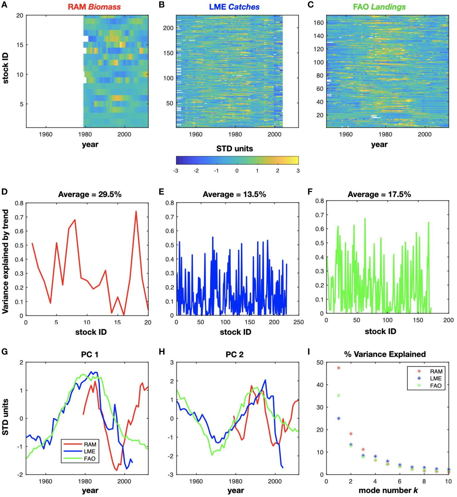
Figure 1 Timeseries of detrended and normalized fish stocks for the RAM (A), LME (B), and FAO (C) datasets. The variance explained by the removed trend is represented in (D, E), and (F). The mean variance excluded by the detrending has been inserted in the plots. The associated variability is described by the first and second principal component (G) and (H), while the corresponding EOFs are displayed in Supplementary Figure S1. The percentage of variance explained by the PCs in each dataset is shown in (I).

The second database considered was the commercial catches from a database aggregated by Large Marine Ecosystem (LME), https://www.lmehub.net/, [Cornillon, Peter. (2007)] (Figure 1B). An LME is defined as an area of 200,000 km² or greater whose extent is determined by similarities in relevant variables such as bathymetry, productivity, or trophic relationships [Sherman, 2014]. The database contains 10,438 stocks in all regions of the world with 55 years of data, from 1950 to 2004. Three LMEs were considered in this study (the Kuroshio, the Oyashio Current and the Sea of Japan LMEs), and those included catches for 225 stocks that have data gaps for less than 5 years. The catches were defined as the weight of fish caught in the open sea independently of the way they have been taken (i.e., gear type or as target or non-target catch). We have considered catches data from 1959 to the most recent data. Here, catches in FAO region 61 (Figure 1J) were analyzed (a region of the Northwest Pacific from about 20°CN to 65°CN and from the coast of Vietnam east to the Bering Strait). The discarded fish have not been filtered out in the two databases; the stocks of the LME database are referred as “catches” as the database contains more catches in weight than the FAO database.

The last database considered included the landings obtained from the Food and Aquaculture Organization (FAO) of the United Nations (https://www.fao.org/fishery/en/statistics) [Pauly et al., 1998] (Figure 1C). Landings for each region offer insight into variability in commercial fishing operations and the fish populations that support them. WE have used 171 landings data with data gaps less than 5 years. As for the LME database we have started the data from 1959.

The stocks considered for the landings and the catches are displayed in Tables 1, 2 and 3 of Supplemental Materials.

2.3 Detrending and standardization

Before proceeding in developing the LIM, we detrended the fisheries and physical time series so to increase their stationarity (i.e., no linear trends are present in any record).

Specifically, the time series extracted from the fisheries databases were standardized by dividing by the standard deviation for each individual stock ID and detrended by removing the best linear trend fit. Consequently, the time series are represented in STD units, and the total number of fish species is described by the StockID (Figures 1A - C). The fish information relative to the fish stocks are provided in Table 1, 2, and 3 of the Supplemental Materials. To examine the percentage of variance excluded by the detrending, we calculated the difference in variance between the total original data and the detrended time series. The mean variance explained by the trend is 29.5% for the RAM biomass (Figure 1D). In particular, the Red seabream Inland sea of Japan (stockID 18) displays the highest variance associated with the trend. For the LME catches and the FAO landings, the variance excluded by removing the trend is 13.5% and 17.5% respectively, as displayed in Figures 1E, F. The associated sign of the removed trend displays a mixture of positive and negative trends in the stock time series of all the three databases (see supplemental Figure S1).

2.4 Principal components and empirical orthogonal functions

To reduce the dimensionality of the detrended and standardized fish indicators, we have used a classic principal components (PCs) analysis. To extract the PCs we first compute the covariance matrix of each fish dataset F_i(s,t), where s denotes the stock id, t its time values, and i the dataset label:

$$C(s,s)={\text{F}}_i(s,t){\text{F}}_i{(t,s)}^T$$

By performing an eigenvalue decomposition of C(s,s),

$${\text{E}}_i(s,k)\text{Λ}(k,k){\text{E}}_i{(k,s)}^T={\text{C}}_i(s,s)$$

we derive the eigenvector E_i(s,k) for the eigenmodes k=1…K where K=7 or RAM, and K=8 for LME and FAO that are associated with the K largest eigenvalues λ(k)  from the diagonal of the eigenvalue matrix Λ(k,k) . The choice of K modes retained in each dataset is explained in section 2.5. Physically, these eigenvectors, referred to as the Empirical Orthogonal Functions (EOFs), are the dominant patterns of variance across the stocks and provide an orthogonal basis onto which we can decompose the original fish datasets as:

$${\text{P}}_i(k,t)={\text{E}}_i{(k,s)}^T{\text{F}}_i(s,t)$$

where P_i(k,t) are the PCs for each dataset i. Using this approach we reduce the dimensionality of the fish dataset from s(order ~100)→k(order ~10) Prior to the computation of the covariance, years with missing data in any given stock were set to zero to void any contribution to the covariance. Given that for any given year there were only few missing data across all the stocks, the impact of setting to zero the missing values has negligible impact the estimation of the EOFs.

The first two dominant PCs for each of the fish dataset are reported in Figures 1G, H and are discussed further in the results section 3.1. The EOFs structures for the first two modes are reported in supplemental material Figure S1.

By normalizing the eigenvalue om the EOFs decomposition, we measure the fraction of variance explained by each pair of PC/EOF mode k as $\lambda (k)/\sum _1^K\lambda (k)$. The spectrum of explained variance is reported in Figure 1I.

2.5 Linear inverse model and forecast

Inverse modeling can be defined as the extraction of dynamical properties of a physical-biological system from its observed statistics. The LIM model suggests that on interannual time scales, our system may be viewed as a linear system driven by Gaussian white noise. The idea is that the climate timescales underpinning the dynamics of our system are longer than the noise. An example of noise are the fast air sea interactions. In this framework the N component state vector of anomalies X volves accordingly to the linear equation,

$\begin{array}{ll}\frac{dX\text{(t)}}{dt}=LX\text{(t)}+\xi \text{(t)}& (1)\end{array}$

In this equation L represents a matrix that describes the feedback among different components of X while ξ  is the stochastic forcing term.

For the purpose of this study, the components of the state vector X and of the operator L in equation (1) are:

$\begin{array}{ll}\frac{dX(t)}{dt}=\left[\begin{array}{c}X{(t)}_{fishery}\\ X{(t)}_{SST}\\ X{(t)}_{SSH}\end{array}\right]=\left[\begin{array}{ccc}{L}_{fishery-fishery}& L_{SST-SSH}& L_{SST-fishery}\\ L_{SSH-SST}& L_{SST-SST}& L_{SSH-fishery}\\ L_{fishery-SST}& L_{SST-SST}& L_{SSH-SSH}\end{array}\right]\left[\begin{array}{c}X{(t)}_{fishery}\\ X{(t)}_{SST}\\ X{(t)}_{SSH}\end{array}\right]+\left[\begin{array}{c}\xi {(t)}_{fishery}\\ \xi {(t)}_{SST}\\ \xi {(t)}_{SSH}\end{array}\right]& (2)\end{array}$

In this framework, the state vector X is made of three substate vectors representing the fishery, SST, and SSH dataset. Each of these substate vectors is constructed using the PCs to reduce the dimensionality of the problem. For example,

$$X{(t)}_{SST}\text{= [}SST\_P{C}_1(t), SST\_P{C}_2(t), \dots . , SST\_P{C}_K(t) ]$$

where K is number of dominant PC retained for each dataset.

In equation (2), the operator L as in the main diagonal the interaction terms of each variable with itself (LSST-SST,Lfisheyr-fishery,LSSH-SSH), while the terms outside the main diagonal are the interaction terms of each variable with the other ones (LSST-SSH,LSST-fishery, LSSH-fishery,LSSH-SST,Lfishery-SST,Lfishery-SSH).

As discussed by Penland et al. [1989], the statistics of a system modeled by the LIM must be Gaussian [Penland et al., 1995]. The operator L can therefore be determined from the state vector X by discretizing the equation (1).

$\begin{array}{ll}L=\frac{1}{\tau }\ln (\langle X(t+\tau )X(t)\rangle \langle X(t)X(t)\rangle )& (3)\end{array}$

After obtaining L we can forecast of the state vector for a specific lead time τ using:

$\begin{array}{ll}\widehat{X}(t+\tau )=\exp (L·\tau )X(t)& (4)\end{array}$

An important assumption in the use of the LIM, and the forecast equation (4), is that the statistics of the system are stationary over the period considered. For this reason, the operator L must be dissipative, which means its eigenvalues must have negative real parts [Newman et al., 2013]. Similarly, we expect that the statistics of stochastic forcing Q=〈ξξ^T〉 [Penland et al., 1995], which are determined from the fluctuations-dissipation relationship,

$\begin{array}{ll}Q=-LC(0)+C(0)L^T& (5)\end{array}$

has positive eigenvalues. In supplemental Figure S2 we have displayed the eigenvalue spectrum for the operator L and the matrix Q We obtain negative eigenvalues for L and positive for Q indicating that our statistics are stationary.

2.5.1 LIM forecast configuration

Number of PCs used in the state vector. To implement the LIM forecast model, the number of PCs retained in the physical and biological state vectors were chosen differently. For the physical components of the analysis, we retain 20 PCs for the SST and 17 for the SSH which capture 77% and 76% of the variance, respectively. These numbers were selected following the configuration of a previous Pacific LIM that uses the same data sources and domain area [see Zhao et al., 2021]. Equation 2 is used independently for each of the fish datasets. To establish how many PCs to retain for each dataset (e.g. RAM, LME, and FAO), we performed a series of cross-validated forecasts (explained in the next section 2.6) using equation (4) to identity the number of biological PCs to retain in the LIM that would lead to the highest forecast skill for the reconstructed fish indicators. Based on this cross-validation, we retained 8 PCs for the RAM biomass, corresponding to 94% of the variance of that quantity, 7 PCs for the LME catches, which describes 74% of the catches total variance, and 7 PCs for the FAO landings, which still correspond to 70% of the variance. Also, for the fishery state vectors, we interpolate the data to the same monthly scale of SST and SSH to allow inclusion of physical information at seasonal time scales.

Temporal span of forecast. The dataset used in this study have different spatial coverage. The physical data is only available starting 1959. Thus, we begin our training of the LIM and examination of the forecast skill over the following period: 1959-2016 for SSTa, 1979-2012 for RAM, 1959-2004 for LME, and 1959-2014 for FAO.

2.6 Cross-validation

To ensure that the LIM is tested on independent data, the estimates of L and of forecasting skills were cross validated by subsampling the data record. We have removed in total 10% of the data, for both the fishery and the physical part, and computed the operator L for the remaining data. The independent years removed are then forecasted using the computed L. This procedure is repeated for the entire period. The associated forecasting skills are computed by the correlation r(τ) between the observational data and the forecast for the different lead times τ For example, to evaluate r(τ) for the each of the fish datasets, the PCs of the forecasted substate vector $\widehat{X}{(\tau )}_{fishery}$ obtained from (eq. 4) [Newman et al., 2003] are projected into the truncated EOF space,

$${\widehat{\text{F}}}_i(s,\tau )={\text{E}}_i{(s,k)}^T{\widehat{\text{P}}}_i(k,\tau )$$

to obtain the forecasted fishery time series that are then correlated with the original data F_i(s,τ) We apply this procedure to the LIM that (1) contains only the physical state variables SST and SSH, and (2) contains the physical variables plus the fishery’s principal components.

2.7 LIM τ est

To test the validity of linear approximation of the LIM, we perform the so called a τ test, which is designed to test the ability of the LIM to reproduce the lag covariance statistics using a lag which goes far beyond the training τ=3 months . Practically, the test consists of comparing the covariance matrix obtained from the original state vector to the covariance matrix calculated using the LIM for different lags τ=3 .. 12 .. 36 months . The LIM is re-computed each time using the different training τ Given that the LIM must be independent of the chosen lag, these two covariance matrices should give a compatible result for the LIM to perform well [Newman et al., 2011; Newman and Sardeshmukh, 2017]. A comparison of the diagonal elements of the observed lag covariances with the one obtained from the LIM is show in the supplemental material for the SST (Figure S3), and each of the fishery datasets (Figures S4–S6). Overall, LIM is able to capture the main structures of the lag autocovariance pattern for both the SST (Figure1 of Supplemental Materials) and the fishery indicator (Figure 2-4 of Supplemental Material) for lags up to τ=72 months in the fish dataset.Results from this test indicate that the LIM approximation is valid for long-lead forecasts of this set of physical and fishery indicators.

2.8 Persistence and forecast skill

When evaluating the skill of a forecast it is customary to ask the question of whether the forecast model adds skill beyond the so-called persistence forecast. This is equivalent to forecasting that each future conditions is the same as the condition today. From a mathematical point of view the persistence correlation forecast skill at different lead time τ for a timeseries y(t). given by the auto-correlation function

$\begin{array}{ll}ACF(\tau )=\frac{y(0)y(\tau )}{y(0)y(0)}& (\mathrm{})\end{array}$

where y(0)y(0) is the covariance at zero lag and y(0)y(τ) is the covariance at lag τ.

In climate science, for a forecast model to have higher skill that persistence is a fundamental measure to indicate that the model is able to extend the predictability through its dynamics beyond the natural temporal auto-correlation that exists in the data. A recent discussion of the concept of persistence can also be found in Jacox et al. [2020]. In the article, we compare the LIM forecast skill to persistence as a way to estimate the LIM’s ability to capture the dynamics of the system and to use those dynamics to extend the predictability of the fish indicators. Specifically, we use the following definitions for the correlation skill,

$\begin{array}{ll}{r}_{Persistence}(\tau )=ACF(\tau )& (\mathrm{})\end{array}$

$$r_{Forecast}(\tau )=\text{correlation(} \widehat{y}(\tau ), y(\tau ))$$

where $\widehat{y}(\tau )$ is the LIM forecasted state at lead τ and $\widehat{y}(\tau )$ is the observed state. As reported in section 2.6, all the forecasted states use a LIM that is trained with a dataset that does not include the observed state, which we also refer to this as the cross-validated forecast skill.

To estimate the statistical significance of the correlation skill we have used a Montecarlo approach. Specifically, we first develop an auto-regressive model of order 1 (AR1) as a null-hypothesis simulation model (i.e., red noise) for a given pair of timeseries that are being compared in the correlation. Next, for each of the timeseries we estimate the lag-1 auto-correlation coefficient and use that to generate 2000 pairs of red noise timeseries using the AR1 model. We compute the probability distribution function (PDF) of correlation coefficients between the red noise timeseries pairs. This PDF is then used to estimate the 95% and 99% confident levels of the correlation between the two original timeseries.

3 Results and discussion

3.1 Fisheries biomass data and relation to physical quantities

Given that the data has been decomposed in EOFs and PCs we first perform an inspection of their statistics. The temporal evolution of the first two dominant modes for the fish datasets are captured by the PC1 and PC2 (Figures 1G, H). Both the PCs1 and PCs2 displays very strong low-frequency variability in each dataset with a significant level of coherency across the datasets. As further discussed in the next sections, these low-frequency variations may be associated not only with decadal climate variability, but also with human influences. For example, these stocks have been heavily exploited in the last 60 years [Pons et al., 2017]. In particular, the increase in fishing pressure coupled with the demography of the fish stocks has led to a collapse and recovery of populations with common trends among stocks as discussed by previous authors [Myers and Worm, 2003; Nye et al., 2009; Wang et al., 2020]. The amount of variance explained by the first two PCs for each fisheries databases (see Methods section 2.4) is very large (Figure 1I). For example, PC1 for the RAM biomass represents 47% of the total variance, while the PC1 of the LME catches and the FAO landings describe respectively 25% and 35% of the variance. This indicates that despite the large number of fish stock indicators, the overall degrees of freedom in the datasets are low and represented by a relatively low number of modes (e.g. pairs of PCs/EOFs).

To quantify the extent to which the low-frequency fluctuations of the fish indicators are tracking climate variability, we perform a correlation analysis between the PCs of the fisheries data and large scale SSTa. Correlations between SST anomalies and the PCs1 for the three fish datasets are reported in Figure 2A. While the patterns show some differences it is evident, especially for the LME and FAO, that stronger correlation existing the region of the KOE. This is more evident by computing a map of the mean correlations across the datasets (Figure 2B), which shows a strong negative correlation from the East China Sea and coastal Japan extending in the central North Pacific. A similar correlation analysis for the PCs2 (Figure 2C) reveals the emergence of the more familiar basin-scale pattern of Pacific decadal variability such as the PDO across all the datasets. Again, this PDO-like pattern becomes clearer in the map of the mean correlations for PCs 2 (Figure 2D) exhibiting strong correlations in the canonical center of actions of the PDO over the central and eastern North Pacific. The correlation patterns of the PCs with the SSTa (Figure 2) gives us confidence that the link between the climate variability and the fish can be exploited for forecasting, especially in the KOE region, where previous studies have shown longer-lead multi-year predictability (see next section 3.2).

FIGURE 2

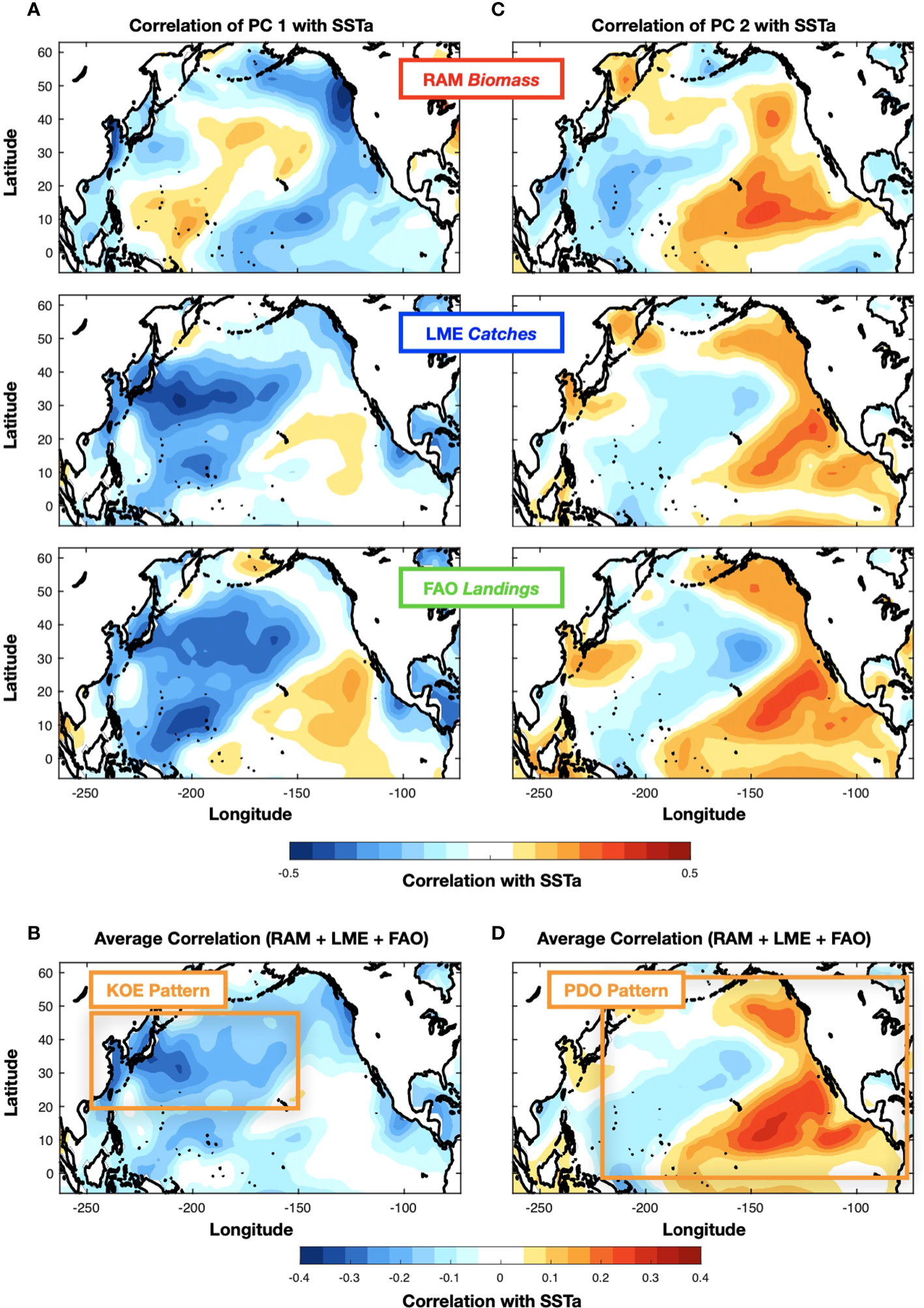
Figure 2 Correlation map between SST anomalies and PC1 (A) and PC2 (C) of the fishery datasets (RAM, LME, FAO). The average correlation maps across the datasets for PC1 and PC2 are shown in (B) and (D).

3.2 LIM forecasts of the low-frequency variability of the KOE

It is well known that the KOE variability is strongly linked to wind induced Rossby waves formed in the Central North Pacific [Deser et al., 1999; Schneider and Miller, 2001; Seager et al., 2001]. The effect of the wave propagation can be separated into two dynamical modes of variability. The first mode is related to a latitudinal shift of the KOE jet, while the second is associated with a strengthening or weakening of the KOE quasi-stationary meanders [Taguchi et al., 2007; Taguchi et al., 2014; Ceballos et al., 2009]. These dynamical changes in the KOE jet can impact the local marine populations with changes in the wintertime mixing and springtime stratification that control seasonal nutrients and light supply for primary producers [Chiba et al., 2013; Nakata et al., 2003]. Given that it takes approximately 2-3 years for the Rossby waves to propagate in the KOE region, these large-scale dynamics carry an inherent multi-year predictability that can be exploited for longer lead low-frequency forecasts on physics and marine ecosystems.

Thus, before exploring the predictability of the fisheries time series, it is informative to quantify the low-frequency predictability of the KOE physical environment, specifically the SST, which is a state variable with strong links to the dynamics of fish populations.

For this purpose, we build a LIM using only SSTa and SSHa data (see Methods section 2.5) and use equation (4) to perform a series of cross-validated forecasts for lead times of 6, 12, and 24 months (Figures 3A, B, C). We find that areas of higher skill are concentrated along the Northeast Pacific coast and the KOE extension and are co-located with centers of actions of the PDO and the KOE low-frequency variability patterns [Matsumura et al., 2016]. We also examine the forecast skill in the KOE region (the average SSTa in the black box of Figure 3A) as a function of the month used to initialize the forecast (Figure 4A). We find that significant forecast skill (correlation >0.6) extends only up to 1.5 year. If we compare this skill level with that obtain from persistence (Figure 4B), we find that the LIM extends this skill beyond persistence up to 10 months (Figure 4C).

FIGURE 3

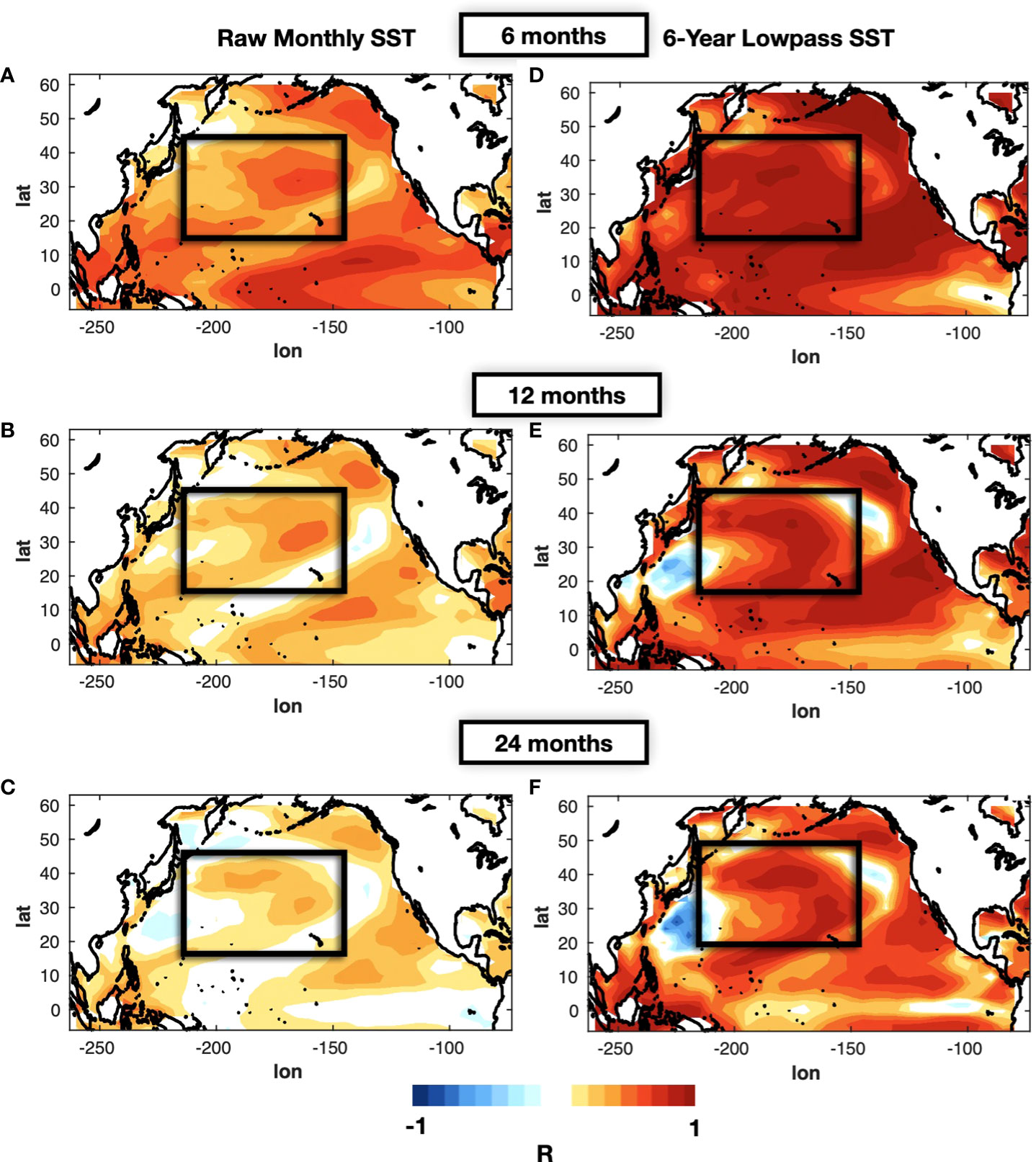
Figure 3 Forecast correlation skill of the LIM with physics only (SSTa, SSHa) for lead-times of 6 months (A), 12 months (B), and 24 months (C). In (D), (E), and (F) the same correlation skill maps are shown but computed using the 6-year low-pass filter applied on the original and forecasted monthly data.

FIGURE 4

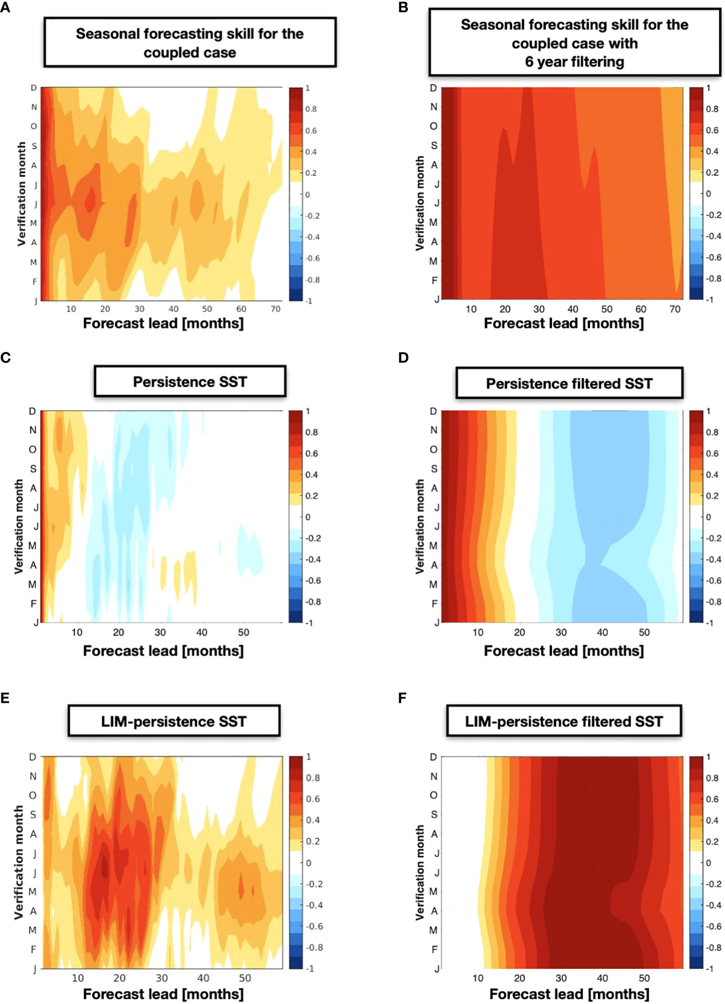
Figure 4 KOE SSTa index forecast correlation skill as a function of the initialization month of the year from the physics only LIM (A), the persistence (B), and their difference (C). The same correlation skill maps are shown but computed after applying a 6-year low-pass filter applied on the original and forecasted monthly data (D, E), and (F).

Given that the fisheries are predominantly characterized by low-frequency variability, we now quantify the low-frequency predictability of the SSTa in the KOE by applying a 6-year filter to the forecasted state vector. As expected when applying a lowpass filter, we find an overall increase in skill spatially at 6, 12, and 24 months (Figures 3D, E, C). If we examine the skill as a function of initialization month (Figure 4D), we find that high skill levels (R>0.6) extends up to lead times of 4-5 years. However, the filtering also leads to longer persistence skill due to the increase in autocorrelation, up to 1.5 years (Figure 4E). Nevertheless, if we look at the difference in skill between the LIM forecast and persistence (Figure 4F), we find that the filtering does extend dynamically the low-frequency predictability by 4-5 years. As emphasized by previous articles [Thompson et al., 2010], the increased skill shows the importance of the low frequency variability of SST anomalies in the KOE jet. These results confirm previous findings that in the KOE, the large-scale climate associated with the propagation of Rossby waves and the modes of decadal variability lead to extended multi-year predictability.

3.3 LIM forecast of fisheries time series

We now analyze if the long-lead, low-frequency predictability of the KOE physical state is important in extending the forecast of fisheries metrics. We construct three independent forecast LIMs for each of the fish datasets (i.e., RAM, LME, FAO) using the definition of the state vector in equation (2) (see Methods section 2.5). The results from the cross-validated forecast are shown in Figures 5A, B, C for leads up to 160 months. Results show high correlation skill values R ~ 0.7 extending almost to the end of the forecast window. Given that stocks are characterized by timeseries with exceptional low-frequency variability, it is critically important to assess If the correlation skill of the LIM is significant. Using the Montecarlo approach discussed in Method section 2.8, we identify the 95% and 99% significance levels for each of the datasets. These are marked in the colorbar of Figure 5 and show that any correlation above R=0.55 (RAM), R=0.41 ((LME), and R=0.44 (FAO) is significant at the 95%. Correlations above R=0.66 (RAM), R=0.51 (LME), and R=0.54 (FAO) are significant at the 99% with the RAM being higher than the other datasets because of its shorten temporal span, which reduced the degrees of freedom.

FIGURE 5

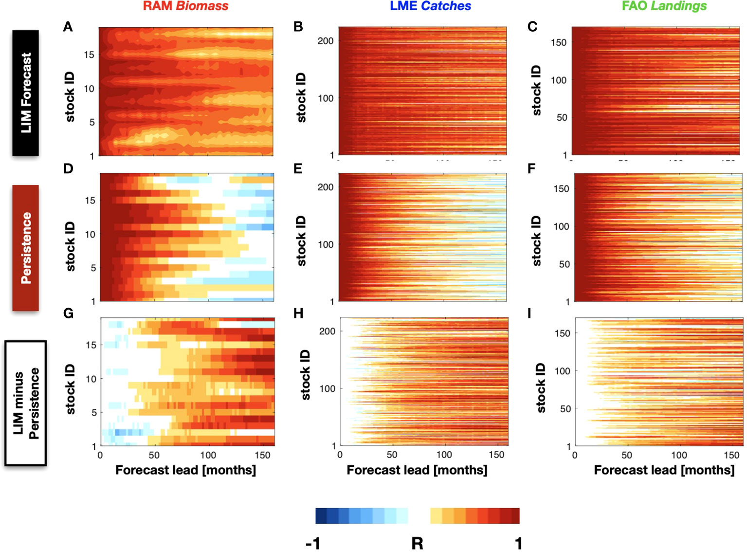
Figure 5 The LIM forecasting correlation skill as a function of different lead-times is displayed from the RAM (A), LME (B), and FAO (C) stocks. The persistence correlation skill for each of these stock is also shown for comparison in (D, E), and (F). A different between the skill of the LIM minus persistence is shown in (G, H), and (I).

We further examine the impact of autocorrelation in the data on the forecast still by computing the persistent forecasts (Figures 5D, E, F). We find significant persistence skill R~0.7 up to 4 years for some of the RAM biomass anomalies (Figure 5D) and up to 3 years for the LME (Figure 5E) catches and FAO landings (Figure 5F). Despite the long-lead forecast skill from persistence, the difference maps between the LIM forecast and persistence skill (Figures 5G, H, I) show that the LIM has higher and extended significant forecast skill beyond the range of persistence by 3-5 year limit.

Despite the statistical measures of skill significance discussed above, it is important to recognize that ultimately the real usefulness of these forecast will depend on how, and what aspects of, this information enables better informed decisions by fishery managers. For this purpose, it is informative to show the timeseries of the LIM forecasts for a few selected species. In each database we picked two species that show extended predictability and displayed their 2- and 5-years composite forecast timeseries (Figure 6, red lines are the cross-validated forecasts, blue line the original data). Focusing on the RAM, Figures 6A, B displays the stock Striped Marlin North Pacific and Yellow sea bream Sea of Japan from the RAM database. Despite the overall higher frequency variability of the LIM forecast, overall the 2-year LIM well captures the low-frequency evolution of the timeseries including some of the interannual extrema on timescale between 2-5 years. In contrast, for longer lead forecasts such as the 5-year (Figures 6C, D), the LIM is only able to capture the low-frequency variations (6 year and above) and loses information about the interannual fluctuations (e.g. compare Figures 6B vs D). A similar behavior is somewhat evident also in the LME catches stocks Sardinops sagax and Reinhardtius evermanni (Figures 6E-H) and the FAO landings stocks Sciaenidae and Colorabis saira (Figures 6I-L). We examine this behavior more systematically across the stocks – that is the LIM loses its ability to forecast interannual fluctuations for longer forecast leads, by applying a 6-year highpass filter on the composite forecasted timeseries for leads times between 0-160 month and re-examine the correlation skill with the original data. We find that the LIM interannual forecast skill is significantly less for longer lead times (Supplemental Figure S7A, B, C) as evident by taking the difference with the non-filtered forecast (Figures S7D, E, F).

FIGURE 6

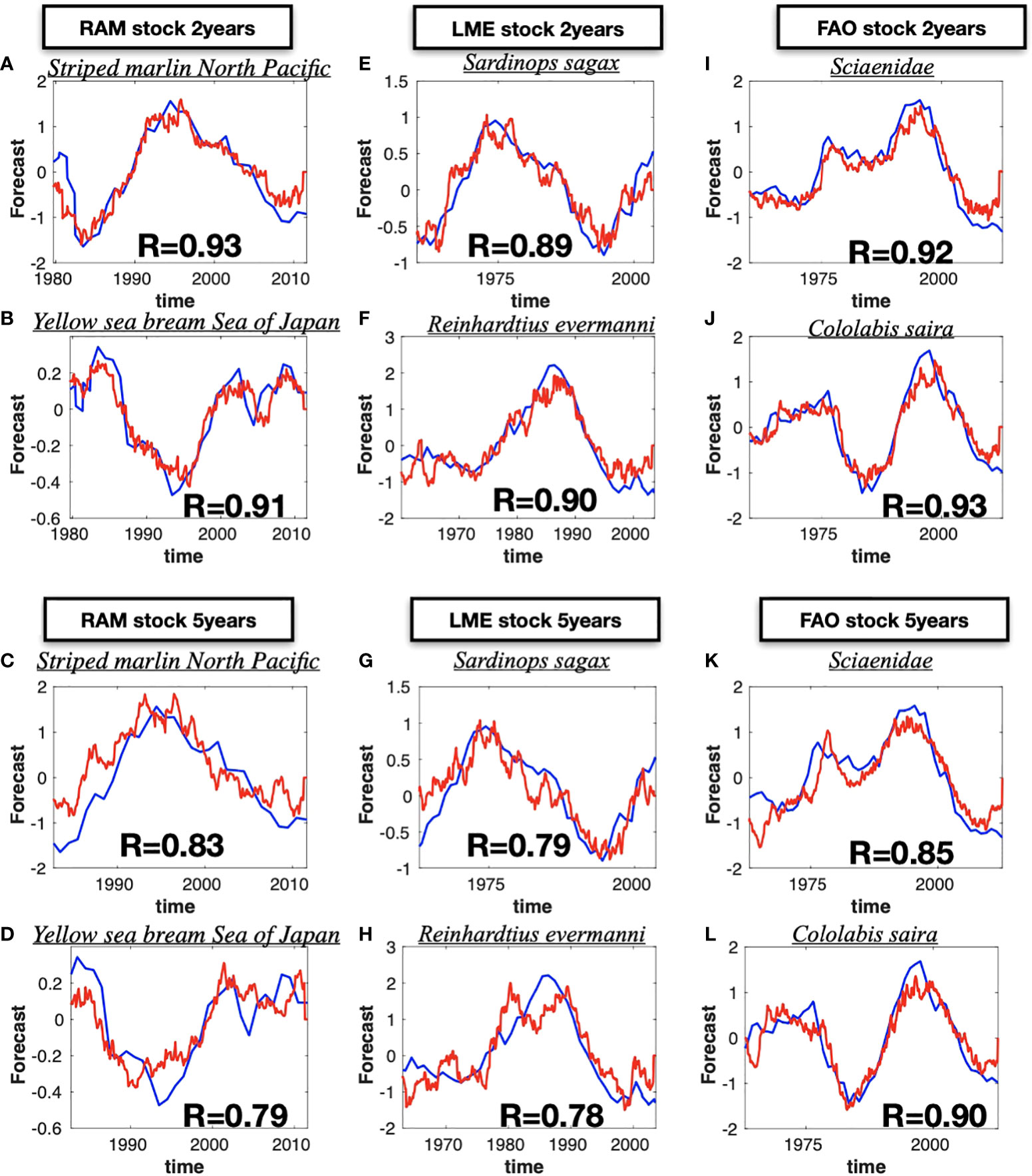
Figure 6 Selected single stock time series (blue lines) and the forecasted time series (red lines). The stock have been selected considering those that have the highest difference between forecasting LIM skill and the persistence. The 2-year lead forecast are shown for the RAM (A, B), for LME(E, F) and for the FAO (I, J). The same comparison are shown for the 5-year lead forecast in panels (C, D) for RAM, (G, H) for LME, and (K, L) for FAO. The name of the selected stock is displayed at the top of each panel.

3.4 LIM forecasting skills sensitivity analysis

To better understand how marine ecosystem components and physical components (and their interaction) contribute to the forecast skill, we perform a sensitivity analysis to investigate key physical and biological factors that influence the predictability of the fisheries. More precisely, the purpose of the sensitivity analysis is to quantify how the forecasting skill of individual fisheries time series depends on knowledge of the climate state and to the knowledge of the other fish stocks.

We begin by exploring the role of the physical state variables in the predictability of the fisheries time series by including the constraint that the interaction terms of the fisheries with SSTa and SSHa in the operator L are zero. This condition implies that we are excluding the interaction of the SSTa and SSHa PCs with the fishery PCs. The forecast skill of the LIM that does not include the coupling with the physics is shown in Figures 7A - C for the different fish datasets. It is immediately apparent that the skill is greatly reduced with compared to the full LIM (Figures 7D–F, show the difference map) suggesting that the information of the phsycial climate variability plays a primary role in extending the LIM forecast skill of the fishery indicators. Specifically, we find that a LIM forecast that depends only on the knowledge of the stock vs. stock interactions (e.g. without the physical information) has limited extended predictability to up to 50 months across the RAM, LME, and FAO timeseries. This reduction in skill can be attributed to several factors, which are not fully investigated in this study. One possible reason regards the role of the Rossby wave propagation in the multiannual prediction of ecological systems [Jacox et al., 2020]. These waves are predominantly initiated in the eastern side of the North Pacific Ocean through modulation of Ekman pumping connected with wind stress curl anomalies induced by the PDO mode [Capotondi and Alexander, 2001; Qiu et al., 2017]. Propagating Rossby waves (RWs) have an important impact on nutrients availability on interannual timescales, which are linked to changes in primary [Sakamoto et al., 2004] and secondary producers as well. In particular, it has been found that RWs modulate the depth of the nutricline by a few tens of meters [Killworth et al., 2004] with corresponding impact on surface nutrient availability. In addition, RW impact surface chlorophyll concentration by a vertical displacement of the chlorophyll maximum, [Dandonneau et al., 2003]. Consequently, it is possible that the exclusion of the physical interactions that are associated with skillful physical predictions from the LIM lead to a much lower forecasting skill for most of the stocks.

FIGURE 7

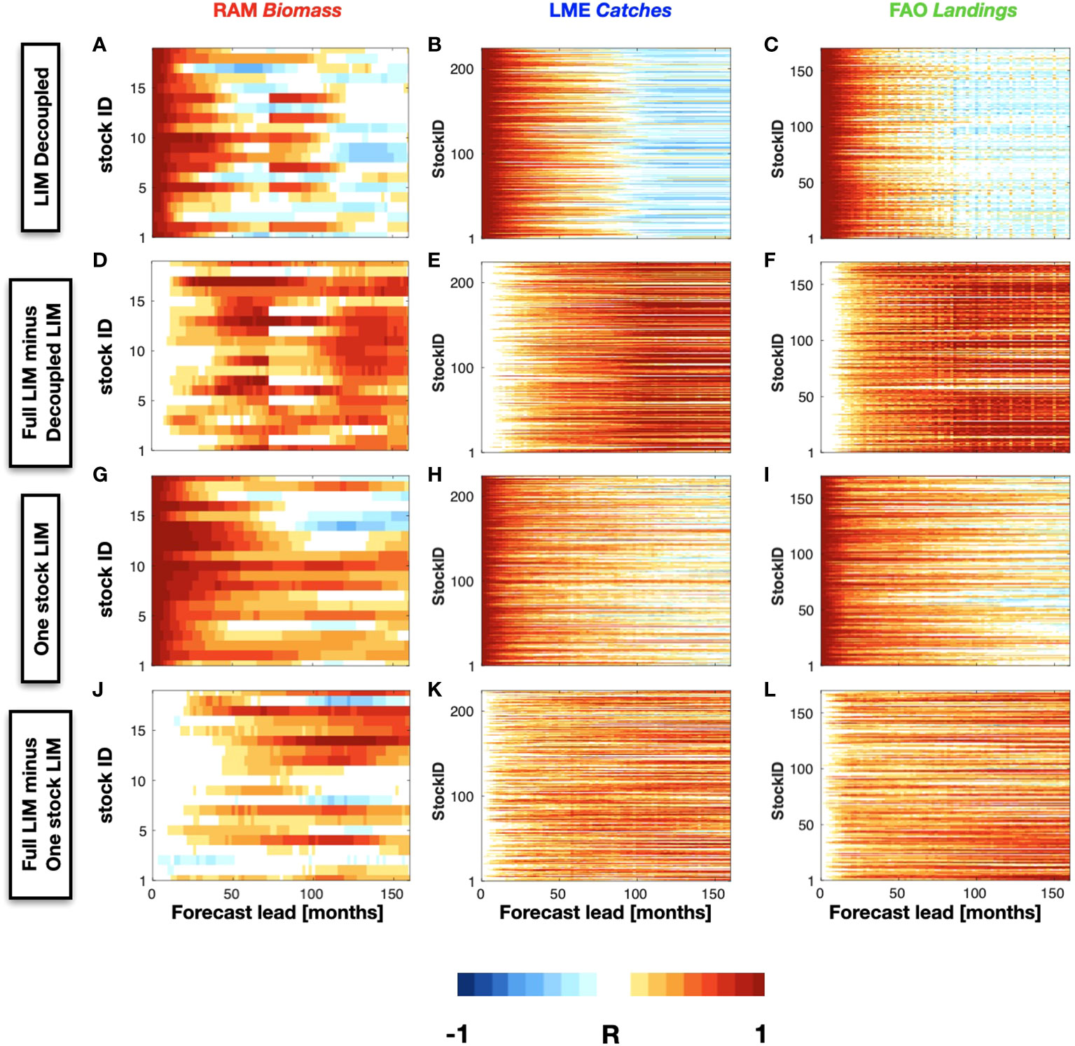
Figure 7 Same as Figure 5, except showing the forecast skill of the LIM where the physics and fish sticks are decoupled, (A) RAM, (B) LME, (C) FAO. The differences in skill between the decoupled and the full LIM case are shown in (D), (E), and (F). The forecasting correlation skill as a function of different lead-times is displayed also for a LIM where each stock is forecasted independently are shown for the RAM (G), LME (H), and FAO (I) datasets, along with the differences from full LIM case in panels (J), (K), and (L), respectively.

Next, we want to examine how the forecast skill depends on the interactions among species. To this end, the full case LIM forecast is repeated by replacing the principal components of the North Pacific stocks with the data time series for each single stock rather than all stocks together (Figures 7G–I). For each of the three databases, the RAM biomass, the FAO landings, and the LME catches, we find again substantial reduction in forecast skill when data from other stocks are excluded from the LIM (Figures 7K–M, show the difference map). This suggest that interactions between stocks contains information that is useful for predictability.

Through these sensitivity analysis, we conclude that the climate forcing has a considerable impact on the fisheries forecast, but it does not represent the only contribution to the skill. To a lesser extent, skill is contributed from the fisheries data from other stocks in the region.

4 Conclusions

Previous studies [Brander et al., 2007; Yati et al., 2020] have documented how climate variability and change have a significant impact on marine populations and fish species in the North Pacific. However, the mechanisms linking climate fluctuations to the dynamics of marine ecosystems are not fully understood and are currently not well captured by numerical models. Long-term timeseries of data for both climate and fisheries such as population biomass (RAM), catches (LME), and landings (FAO) provide an opportunity to explore the coupled climate-fish predictability using empirical dynamical models and machine learning approaches. These approaches are very promising because the time series of fish indicators also reflect non-climate forcings that are related to the internal stock dynamics, human exploitation by commercial fishing, economic conditions, and technological advancements. These combined interactions are hard to resolve in traditional dynamical models. Each of these non-climate processes and their interactions, can have a substantial influence on metrics of fisheries biomass, landings, and catches. However, the relative importance of these factors on the variability of fish species and their predictability has not been fully explored.

In this paper, we used observationally derived lag covariance statistics to empirically capture the linear and (fast) nonlinear interactions among fish stocks, and of fish stocks with human and climate drivers (e.g. the LIM forecast model). Our results showed that the empirical dynamical forecast of the climate-fish-human multi-variate LIM has long-lead predictability that extends beyond the persistence timescale for up to 5-years with significant skill. This finding is consistent with recent studies showing how both short-lived and long-lived species display a response to climate variability and to the increased fishing pressure [Pinsky and Byler, 2015; Rouyer et al., 2014; Wang et al., 2020]. To further confirm and separate the impacts that climate and non-climate drivers are having on the fisheries, we have implemented a series of sensitivity analyses that selectively included or excluded the interaction terms between climate and fisheries time series in the LIM dynamical operator. Results of the analysis revealed a significant decrease in fish forecast skill when the interaction with the SSH and SST is excluded. While the LIM methodology does not allow us to explicitly diagnose which mechanisms of physical-biological coupling are important for extending the predictability in the KOE region, it does confirm and quantify the critical role of ocean climate dynamics, which previous studies had discussed but not explored with rigorous quantitative measures [see also review from Jacox et al., 2020]. In fact, this study is to our knowledge one of the first attempt to explore empirical model forecasting in the KOE region.

Further analyses also revealed that the forecast skill arising from empirical relationships among the stocks are also important, although less important than the inclusion of physical characteristics. This indicates that the information shared among stocks, which could be reflective of changes in industrial fishing practices, market forces, or species interactions, substantially improves forecasting skill. In particular, we notice a distinction in the RAM data between short-lived species and long-lived species as we compare the results with the first sensitivity analysis. Short living species are highly dependent on the climate factors and much less on the stock-stock interactions. While long-living species have a dependency on climate factors of the North Pacific, but the stock-stock interactions give a high contribution as well to the forecasting skill much more than short living species.

Although more studies are required to understand the joint predictability dynamics between climate and fisheries In the Pacific Ocean, the analyses presented here with a multivariate linear inverse model provide a promising approach for utilizing climate information to predict socio-ecological indicators such as fish catch, biomass, and landings. Our results also suggest that this approach may be successful in accounting for the dynamics of external human forcing (e.g., in this case fishing) that are implicitly incorporated in the stock-stock interaction terms. Lastly, these findings support the idea that predicting the marine ecosystem as a hole (e.g., including multi-variate ecological indicators) is more skillful than focusing on individual stock timeseries.

Data availability statement

The original contributions presented in the study are included in the article/supplementary material. Further inquiries can be directed to the corresponding author.

Author contributions

The authors confirm contribution to the paper as follows: study conception and design: GN, EL. Data collection: GN. Analysis and interpretation of results: GN, EL, RR, AC. Draft manuscript preparation: GN, EL, RR, AC. All authors contributed to the article and approved the submitted version.

Acknowledgments

The work is supported by the Leatherback Trust funds in the Ocean Science and Engineering program at the Georgia Institute of Technology, and was partially supported by the Department of Energy (DOE) RGMA grant DE‐SC0019418 and the NSF CCE-LTER. We want thank Dr. Yingying Zhao for helping with the processing of the SST and SSH reanalysis data. No conflicts of interest are present.

Conflict of interest

The authors declare that the research was conducted in the absence of any commercial or financial relationships that could be construed as a potential conflict of interest.

Publisher’s note

All claims expressed in this article are solely those of the authors and do not necessarily represent those of their affiliated organizations, or those of the publisher, the editors and the reviewers. Any product that may be evaluated in this article, or claim that may be made by its manufacturer, is not guaranteed or endorsed by the publisher.

Supplementary material

The Supplementary Material for this article can be found online at: https://www.frontiersin.org/articles/10.3389/fmars.2022.969319/full#supplementary-material

References

Blanchard J. L., Coll M., Trenkel V. M., Vergnon Rémi, Yemane D., Jouffre D., et al. (2010). Trend analysis of indicators: a comparison of recent changes in the status of marine ecosystems around the world. ICES J. Mar. Sci. 67, Issue 4, 732–744. doi: 10.1093/icesjms/fsp282

CrossRef Full Text | Google Scholar

Bograd S. J., Kang S., Di Lorenzo E., Horii T., Katugin O. N., King J. R., et al. (2019). Developing a social–Ecological–Environmental system framework to address climate change impacts in the north pacific. Front. Mar. Sci. 6. doi: 10.3389/fmars.2019.00333

CrossRef Full Text | Google Scholar

Brander K. M. (2007). Global fish production and climate change. Proc Natl Acad Sci USA 104 (50), 19709–14. doi: 10.1073/pnas.0702059104

PubMed Abstract | CrossRef Full Text | Google Scholar

Capotondi A., Alexander M. A. (2001). Rossby waves in the tropical north pacific and their role in decadal thermocline variability. J. Phys. Oceanography 31 (12), 3496–3515. doi: 10.1175/1520-0485(2002)031<3496:RWITTN>2.0.CO;2

CrossRef Full Text | Google Scholar

Capotondi A., Jacox M, Bowler C, Kavanaugh M, Lehodey P, Barrie D, et al. (2019). Observational needs supporting marine ecosystem modeling and forecasting: Insights from U.S. Coast. Appl. Front. Mar. Sci 6:623. doi: 10.3389/fmars.2019.00623

CrossRef Full Text | Google Scholar

Capotondi A., Newman M., Xu T., Di Lorenzo E. (2022). An optimal precursor of northeast pacific marine heatwaves and central pacific El niño events. Geophysical Res. Lett. 49, e2021GL097350. doi: 10.1029/2021GL097350

CrossRef Full Text | Google Scholar

Ceballos L. I., Di Lorenzo E., Hoyos C. D., Schneider N., Taguchi B. (2009). North pacific gyre oscillation synchronizes climate fluctuations in the Eastern and Western boundary systems. J. Climate 22 (19), 5163–5174. doi: 10.1175/2009JCLI2848.1

CrossRef Full Text | Google Scholar

Cornillon P (2007). Fronts in the World Ocean's Large Marine Ecosystems. 21

Google Scholar

Chavez F. P., Ryan J., Lluch-Cota S., Niquen M. (2003). From anchovies to sardines and back: Multidecadal change in the pacific ocean. Science. 299, 217–221. doi: 10.1126/science.1075880

PubMed Abstract | CrossRef Full Text | Google Scholar

Chiba S., Di Lorenzo E., Davis A., Keister J. E., Taguchi B., Sasai Y., et al. (2013). Large-Scale climate control of zooplankton transport and biogeography in the kuroshio-oyashio extension region. Geophys. Res. Lett. 40, 5182–5187. doi: 10.1002/grl.50999

CrossRef Full Text | Google Scholar

Dandonneau Y., Vega A., Loisel H., du Penhoat Y., Menkes C. (2003). Oceanic rossby waves acting as a "hay rake" for ecosystem floating by-products. Science. 302 (5650), 1548–1551. doi: 10.1126/science.1090729

PubMed Abstract | CrossRef Full Text | Google Scholar

Deser C., Alexander M., Timlin M. (1999). Evidence for a wind-driven intensification of the kuroshio current extension from the 1970s to the 1980s. J. Climate - J. CLIMATE. 12, 1697–1706. doi: 10.1175/1520-0442(1999)012<1697:EFAWDI>2.0.CO;2

CrossRef Full Text | Google Scholar

Di Lorenzo E., Schneider N., Cobb K. M., Franks P. J. S., Chhak K., Miller A. J., et al. (2008). North pacific gyre oscillation links ocean climate and ecosystem change. Geophys. Res. Lett. 35, L08607. doi: 10.1029/2007GL032838

CrossRef Full Text | Google Scholar

Di Lorenzo E., Ohman M. (2013). A double-integration hypothesis to explain ocean ecosystem response to climate forcing. Proc. Natl. Acad. Sci. United States America 110, 2496–99. doi: 10.1073/pnas.1218022110

CrossRef Full Text | Google Scholar

Jacox M., Alexander M., Siedlecki S., Chen Ke, Kwon Y.-O., Brodie S., et al. (2020). Seasonal-to-interannual prediction of U.S. coastal marine ecosystems: Forecast methods, mechanisms of predictability, and priority developments. Prog. Oceanography. 183, 102307. doi: 10.1016/j.pocean.2020.102307

CrossRef Full Text | Google Scholar

Kelly K. A., Small R. J., Samelson R. M., Qiu B., Joyce T. M., Kwon Y., et al. (2010). Western Boundary currents and frontal air–Sea interaction: Gulf stream and kuroshio extension. J. Climate 23 (21), 5644–5667. doi: 10.1175/2010JCLI3346.1

CrossRef Full Text | Google Scholar

Killworth P. D., Cipollini P., Uz B. M., Blundell J. R. (2004). Physical and biological mechanisms for planetary waves observed in satellite-derived chlorophyll. J. Geophys. Res. 109, C07002. doi: 10.1029/2003JC001768

CrossRef Full Text | Google Scholar

Koul V., Sguotti C., Årthun M., Brune S, Düsterhus A, Bogstad B, et al. (2021). Skilful prediction of cod stocks in the north and barents Sea a decade in advance. Commun. Earth Environ. 2, 140. doi: 10.1038/s43247-021-00207-6

CrossRef Full Text | Google Scholar

Kwon Y. O., Alexander M, Bond NA, Frankignoul C, Nakamura H, Qiu B, et al. (2010). Role of the gulf stream and kuroshio-oyashio systems in Large-scale atmosphere-ocean interaction: A review. J. Climate 23 (12), 3249–3281. doi: 10.1175/2010JCLI3343.1

CrossRef Full Text | Google Scholar

Lin P., Chai F., Xue H., Xiu P. (2014). Modulation of decadal oscillation on surface chlorophyll in the kuroshio extension. J. Geophys. Res. Oceans 119, 187–199. doi: 10.1002/2013JC009359

CrossRef Full Text | Google Scholar

Liu Z., Di Lorenzo E. (2018). Mechanisms and predictability of pacific decadal variability. Curr. Clim Change Rep. 4, 128–144. doi: 10.1007/s40641-018-0090-5

CrossRef Full Text | Google Scholar

Mantua N. J., Hare S. R., Zhang Y., Wallace J. M., Francis R. C. (1997). A pacific interdecadal climate oscillation with impacts on salmon production. Bull. Am. Meteorol. Soc 78, 1069–1079. doi: 10.1175/1520-0477(1997)078<1069:APICOW>2.0.CO;2

CrossRef Full Text | Google Scholar

Matsumura S., Horinouchi T. (2016). Pacific ocean decadal forcing of long-term changes in the western pacific subtropical high. Sci. Rep. 6, 37765. doi: 10.1038/srep37765

PubMed Abstract | CrossRef Full Text | Google Scholar

Mitsudera H., Waseda T., Yoshikawa Y., Taguchi B. (2001). Anticyclonic eddies and kuroshio meander formation. Geophys. Res. Lett. 28, 2025–2028. doi: 10.1029/2000GL012668

CrossRef Full Text | Google Scholar

Mizuno K., White W. B. (1983). Annual and interannual variability in the kuroshio current system. J. Phys. Oceanogr. 10, 1847–1867. doi: 10.1175/1520-0485(1983)013<1847:AAIVIT>2.0.CO;2

CrossRef Full Text | Google Scholar

Möllmann C., Diekmann R. (2012). Marine ecosystem regime shifts induced by climate and overfishing. Adv. Ecol. Res. Glob. Change Multispecies Syst. 47, 303–347. doi: 10.1016/b978-0-12-398315-2.00004-1

CrossRef Full Text | Google Scholar

Myers R., Worm B. (2003). Rapid worldwide depletion of predatory fish communities. Nature 423, 280–283. doi: 10.1038/nature01610

PubMed Abstract | CrossRef Full Text | Google Scholar

Nakata K., Hidaka K. (2003). Decadal-scale variability in the kuroshio marine ecosystem in winter. Fisheries Oceanography 12, 234–244. doi: 10.1046/j.1365-2419.2003.00249.x

CrossRef Full Text | Google Scholar

Newman M. (2007). Interannual to decadal predictability of tropical and north pacific Sea surface temperatures. J. Climate 20 (11), 2333–2356. doi: 10.1175/JCLI4165.1

CrossRef Full Text | Google Scholar

Newman M. (2013). An empirical benchmark for decadal forecasts of global surface temperature anomalies. J. Climate 26 (14), 5260–5269. doi: 10.1175/JCLI-D-12-00590.1

CrossRef Full Text | Google Scholar

Newman M., Alexander M., Scott J. (2011). An empirical model of tropical ocean dynamics. Climate Dynamics. 37, 1823–1841. doi: 10.1007/s00382-011-1034-0

CrossRef Full Text | Google Scholar

Newman M., Sardeshmukh P. D. (2017). Are we near the predictability limit of tropical indo-pacific sea surface temperatures? Geophys. Res. Lett. 44, 8520–8529. doi: 10.1002/2017GL074088

CrossRef Full Text | Google Scholar

Newman M., Sardeshmukh P. D., Winkler C. R., Whitaker J. S. (2003). A study of subseasonal predictability. Monthly Weather Rev. 131 (8), 1715–1732. doi: 10.1175//2558.1

CrossRef Full Text | Google Scholar

Nye J. A., Link J. S., Hare J. A., Overholtz W. J. (2009). Changing spatial distribution of fish stocks in relation to climate and population size on the northeast united states continental shelf. Mar. Ecol. Prog. Ser. 393, 111–129. doi: 10.3354/meps08220

CrossRef Full Text | Google Scholar

Park J. Y., Stock C. A., Dunne J. P., Yang X., Rosati A. (2019). Seasonal to multiannual marine ecosystem prediction with a global earth system model. Science. 365 (6450), 284–288. doi: 10.1126/science.aav6634

PubMed Abstract | CrossRef Full Text | Google Scholar

Pauly D., Christensen V., Dalsgaard J., Froese R., Torres F. Jr (1998). Fishing down marine food webs. Science 279, 860–863. doi: 10.1126/science.279.5352.860

PubMed Abstract | CrossRef Full Text | Google Scholar

Penland C. (1989). Random forcing and forecasting using principal oscillation pattern analysis. Mon. Weather Rev. 10, 2165–2185. doi: 10.1175/1520-0493(1989)117<2165:RFAFUP>2.0.CO;2

CrossRef Full Text | Google Scholar

Penland C., Sardeshmukh P. D. (1995). The optimal growth of tropical Sea surface temperature anomalies. J. Climate 8 (8), 1999–2024. doi: 10.1175/1520-0442(1995)008<1999:TOGOTS>2.0.CO;2

CrossRef Full Text | Google Scholar

Pinsky M. L., Byler D. (2015). Fishing, fast growth and climate variability increase the risk of collapse. Proc. B. 282, 20151053. doi: 10.1098/rspb.2015.1053

CrossRef Full Text | Google Scholar

Pons M., Branch T. A., Melnychuk M. C., Jensen O. P., Brodziak J., Fromentin J. M., et al. (2017). Effects of biological, economic and management factors on tuna and billfish stock status. Fish Fish 18, 1–21. doi: 10.1111/faf.12163

CrossRef Full Text | Google Scholar

Qiu B. (2003). Kuroshio extension variability and forcing of the pacific decadal oscillations: Responses and potential feedback. J. Phys. Oceanography 33 (12), 2465–2482. doi: 10.1175/2459.1

CrossRef Full Text | Google Scholar

Qiu B., Chen S. (2005). Variability of the kuroshio extension jet, recirculation gyre, and mesoscale eddies on decadal time scales. J. Phys. Oceanography 35 (11), 2090–2103. doi: 10.1175/JPO2807.1

CrossRef Full Text | Google Scholar

Qiu B., Chen S., Schneider N. (2017). Dynamical links between the decadal variability of the oyashio and kuroshio extensions. J. Climate 30 (23), 9591–9605. doi: 10.1175/JCLI-D-17-0397.1

CrossRef Full Text | Google Scholar

Ricard D., Minto C., Jensen O. P., Baum J. K. (2012). Examining the knowledge base and status of commercially exploited marine species with the RAM legacy stock assessment database. Fish Fish 13, 380–398. doi: 10.1111/j.1467-2979.2011.00435.x

CrossRef Full Text | Google Scholar

Rouyer T., Fromentin J.-M., Hidalgo M., Stenseth N. C. (2014). Combined effects of exploitation and temperature on fish stocks in the northeast Atlantic. ICES J. Mar. Sci. 71, 1554–1562. doi: 10.1093/icesjms/fsu042

CrossRef Full Text | Google Scholar

Sakamoto C. M., Karl D. M., Jannasch H. W., Bidigare R. R., Letelier R. M., Walz P. M., et al. (2004). Influence of rossby waves on nutrient dynamics and the plankton community structure in the north pacific subtropical gyre. J. Geophys. Res. 109, C05032. doi: 10.1029/2003JC001976

CrossRef Full Text | Google Scholar

Schneider N., Miller A. J. (2001). Predicting Western north pacific ocean climate. J. Clim. 20, 3997–4002. doi: 10.1175/1520-0442(2001)014<3997:PWNPOC>2.0.CO;2

CrossRef Full Text | Google Scholar

Seager R., Kushnir Y., Naik N. H., Cane M. A., Miller J. (2001). Wind-driven shifts in the latitude of the kuroshio–oyashio extension and generation of SST anomalies on decadal timescales. J. Climate 14, 4249–4265. doi: 10.1175/1520-0442(2001)014<4249:WDSITL>2.0.CO;2

CrossRef Full Text | Google Scholar

Sherman K. (2014). Adaptive management institutions at the regional level: the case of large marine ecosystems. Ocean Coast. Manage. 90, 38–49. doi: 10.1016/j.ocecoaman.2013.06.008

CrossRef Full Text | Google Scholar

Shin Y.-J., Shannon L. J., Bundy A., Coll M., Aydin K., Bez N., et al. (2010). Using indicators for evaluating, comparing, and communicating the ecological status of exploited marine ecosystems. 2. setting the scene. ICES J. Mar. Sci. 67, 692–716. doi: 10.1093/icesjms/fsp294

CrossRef Full Text | Google Scholar

Taguchi B., Schneider N. (2014). Origin of decadal-scale, Eastward-propagating heat content anomalies in the north pacific. J. Climate 27 (20), 7568–7586. doi: 10.1175/JCLI-D-13-00102.1

CrossRef Full Text | Google Scholar

Taguchi B., Xie S.-P., Schneider N., Nonaka M., Sasaki H., Sasai Y. (2007). Decadal variability of the kuroshio extension: Observations and an eddy-resolving model hindcast. J. Clim. 20, 2357–2377. doi: 10.1175/JCLI4142.1

CrossRef Full Text | Google Scholar

Tam J., Fay G., Link J. (2019). Better together: The uses of ecological and socio-economic indicators with end-to-End models in marine ecosystem based management. Front. Mar. Science. 6. doi: 10.3389/fmars.2019.00560

CrossRef Full Text | Google Scholar

Thompson L. A., Kwon Y. (2010). An enhancement of low-frequency variability in the kuroshio–oyashio extension in CCSM3 owing to ocean model biases. J. Climate 23 (23), 6221–6233. doi: 10.1175/2010JCLI3402.1

CrossRef Full Text | Google Scholar

Tommasi D., Stock C. A., Alexander M. A., Yang X., Rosati A., Vecchi G. A. (2017). Multi-annual climate predictions for fisheries: An assessment of skill of Sea surface temperature forecasts for Large marine ecosystems. Front. Mar. Sci. 4. doi: 10.3389/fmars.2017.00201

CrossRef Full Text | Google Scholar

Wang J. Y., Kuo T. C., Hsieh Ch. (2020). Causal effects of population dynamics and environmental changes on spatial variability of marine fishes. Nat. Commun. 11, 2635. doi: 10.1038/s41467-020-16456-6

PubMed Abstract | CrossRef Full Text | Google Scholar

Yati E., Minobe S., Mantua N., Ito S., Di Lorenzo E. (2020). Marine ecosystem variations over the north pacific and their linkage to Large-scale climate variability and change. Front. Mar. Sci. 7. doi: 10.3389/fmars.2020.578165

CrossRef Full Text | Google Scholar

Yatsu A., Chiba S., Yamanaka Y., Ito S.-i., Shimizu Y., Kaeriyama M., et al. (2013). Climate forcing and the Kuroshio/Oyashio ecosystem. ICES J. Mar. Sci. 70 (5), 922–933. doi: 10.1093/icesjms/fst084

CrossRef Full Text | Google Scholar

Yunne-Jai S., Lynne J.S. (2010). Using indicators for evaluating, comparing, and communicating the ecological status of exploited marine ecosystems. 1. the IndiSeas project. ICES J. Mar. Sci. 67 (4), 686–691. doi: 10.1093/icesjms/fsp273

CrossRef Full Text | Google Scholar

Zhao Y. Y., Newman M., Capotondi A., Di Lorenzo E., Sun D. X. (2021). Removing the effects of tropical dynamics from north pacific climate variability. J. Climate 34 (23), 9249–9265. doi: 10.1175/jcli-d-21-0344.1

CrossRef Full Text | Google Scholar