The effect of waves in hydrodynamics, stratification, and salt wedge intrusion in a microtidal estuary

Introduction

Estuaries are areas where the exchange of water, sediments, salt, nutrients, and pollutants occurs between land and the ocean, . This exchange depends on the interaction between oceanic, atmospheric, and river drivers, which defines its extension, vertical density structure, and morphology (Prandle et al., 2006; Toffolon et al., 2006; Ma et al., 2015). Most of them are highly populated places, which can bring pollution problems, due to their multiple uses (recreation, ports, fishing, water demand, among others). The study of the physical processes of circulation, stratification, and mixing between river and seawater has been mainly based on field measurements and the application of numerical models where, usually, the effects of waves are neglected, either to simplify the system (Maljutenko and Raudsepp, 2019), or because of the low level of energy they contribute (Jang et al., 2012; Defontaine et al., 2020). In the cases that include the effects of waves on hydrodynamics, stratification or sedimentary dynamics in estuarine systems, it has been found: (i) a decrease in surface flow velocity at the mouth, when the direction between the estuarine outflow jet and the waves is opposite; (ii) differences in the current field, where the waves can generate strong coastal currents; (iv) weakening of stratification due to increased vertical mixing; and (v) changes in sediment deposition and transport due to re-suspension of sediments on the bottom, because of increased shear stress (Bolaños et al., 2014; MacVean and Lacy, 2014; Jia et al., 2015). Such effects are considered relevant for to the most energetic cases of waves (Gong et al., 2018a; Chen et al., 2019).

The main effects of waves on estuarine hydrodynamics have been evaluated using the radiation stress tensor and Stokes drift. In microtidal estuaries, waves have been observed to generate strong littoral currents that affect coastal sediment transport (Davis and Fox, 1981), and wave breaking has been observed to increase the mixing of river and seawater (Dyer, 1991). The decrease in velocity, when the waves propagate against the outflow estuarine current, is accompanied by a rise in water level surface at the mouth and inland of the estuary due to the increased effective friction over the outflow (Bender and Wong, 1993), and by the Stokes drift that causes a buildup of water and momentum landward, resulting in a negative seaward level gradient (Guo et al., 2014). These changes produce variations in hydrodynamics and circulation processes, which in turn can affect sediment deposition patterns at the mouth of estuaries and may be more significant during low freshwater discharges (Zhang et al., 2018). In numerical models, the effects of waves when coupled with water body simulations is addressed through the 2D radiation stress formulation, based on the linear wave theory of Longuet-Higgins and Stewart (1964). Radiation stress is defined as the excess momentum flow due to the presence of waves. The water body model MOHID is coupled in a way with the spectral wave model SWAN, incorporeting to incorporating into MOHID the fields of significant wave height, period, wavelength, direction, wave-induced force (2D radiation stress), and maximal orbital velocity near the bottom (Malhadas et al., 2009; Park et al., 2015).

There are few studies at the Magdalena River estuary (MRE), where the hydrodynamic processes have been analyzed considering the effects of waves, even though it has been classified as a mixed delta dominated by waves and fluvial discharges (Wright, 1977; Wright et al., 1980; Restrepo et al., 2018). Urbano et al. (2013), employed a 2D hydrodynamic model and the SWAN model (Booij et al., 1999) to study the effect of the mean water currents on the waves, showing that the significant wave height is incremented inside of the MRE by the river outflow and as a function of wave direction, with greater penetration when waves are coming from the north. Ospino et al. (2018) studied the variations in saline intrusion in the MRE, using the MOHID 3D numerical model, considering different freshwater discharges and wind conditions, finding that the river flow is the main force in the variation of saline intrusion, but without considering the effects of waves. Otero et al. (2021), based on the results of MOHID 3D, studied the stratification and mixing in the estuary under cold, warm, and neutral ENSO (El Niño Southern Oscillation) conditions, finding that, during the low-flow season, under warm and neutral ENSO conditions, the estuary is salt-wedge type, and salinity intrusion can reach 20 km upstream the mouth under extreme low flow conditions, whereas, during cold ENSO conditions, the estuary is well mixed, fluvial conditions prevail, and mixing processes occur outside the river mouth. The effects of waves on hydrodynamic processes in the MRE were not considered in this case.

Filling The gap, the present work is focused on the effects of waves on hydrodynamics, processes such as stratification, circulation, and salt wedge dynamics are evaluated in the MRE. Field data and the coupling of the 3D MOHID finite volume model (Neves, 1985; Leitão, 2003; Franz et al., 2017), with the SWAN spectral wave model (Booij et al., 1999), previously calibrated and validated, were used. The low freshwater discharge seasons of 2018 and 2020 were taken as case studies, simulating current-only conditions (tidal and river), and comparing the results with simulations that include also the effects of waves on hydrodynamics.

Study area

The Magdalena River estuary is located in northern South America, on the Caribbean coast of Colombia (Figure 1). The Magdalena River generates the largest input of fresh water (205 km³ y^-1) and sediment (144X10⁶ t y^-1) to the Caribbean Sea. More than 90% of the sediment discharged by the river is transported in suspension (Higgins et al., 2016). The system presents flows with high seasonal and interannual variability, with average values of between 9570 m³s^-1, for periods of high discharges (Oct-Nov); 7293 m³s^-1, for medium discharges; and 5090 m³s^-1 on average, for low discharges; with minimums as low as 2800 m³s^-1 (Otero et al., 2021). Under low flow conditions at the mouth, salt wedge intrusion is present, whereas, at high flows, there is no stratification within the delta, and the halocline is found outside the mouth (Ospino et al., 2018; Otero et al., 2021).

FIGURE 1

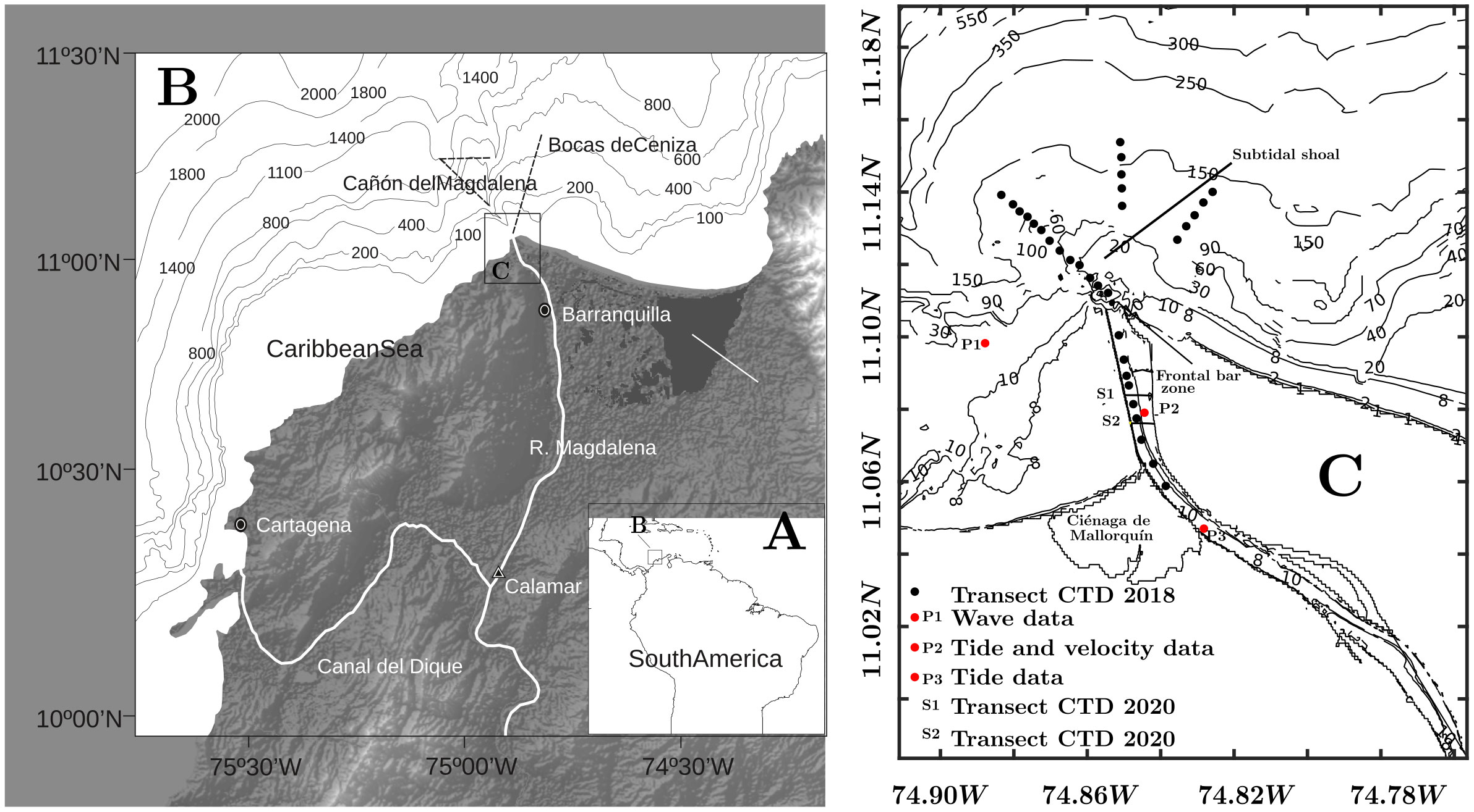
Figure 1 Shows the location of the study zone in (A) South America and Colombia; (B) the mouth of the Magdalena River, showing the location of the engineering structures built along the main channel (1-9) and (C) bathymetry and location of the measuring instruments and longitudinal transepts of the measurements station with CTD in dry seasons 2018, P1 wave data measuring with the Aquadop profiler (12-19-2014 to 01-24-2015), P2 the location of the Nortek Aquadopp profiler and S1 and S2 Cross sections for the 2020 dry season.

The climate in the Colombian Caribbean is characterized by two seasons: a dry season from December to May, and a wet season the rest of the year. The wet season is interrupted by a relatively dry stretch in June and July, known as the Veranillo de San Juan (Poveda and Mesa, 1999; Andrade, 2001). Regarding wind, the multiannual mean velocity at the deltaic front presents high seasonal and interannual variability. Seasonal wind patterns are defined by the latitudinal migration of the intertropical convergence zone (ITCZ) and the trade winds (Poveda, 2004), with speeds of between 0.5 and 12 ms^-1, with maximum speeds of up to 14 ms^-1 in March. During the dry season, the locally waves is dominated by the wind, with significant average heights of 1.5 m, with maximum heights of 3.9 m in the outer zone of the delta (Ortiz et al., 2013; Daniel et al., 2015). During low flow periods (December-March), the most intense winds and local wind wave heights occur at the river mouth (Ortiz et al., 2013). This can generate re-suspension processes in the sediments (e.g. Gallivan and Davis, 1981; Shi et al., 2006), greater mixing in the water column, which can affect vertical stratification patterns, penetration into the salt wedge (Gong et al., 2018a), as well as longitudinal and transverse variations in salinity and density patterns, mainly in the mouth zone.

The MRE is a microtidal estuary, with a tidal range between 0.48 and 0.64 m in neap and spring tide, respectively, of mainly diurnal mixed predominance (F=1.67) (Restrepo et al., 2018). Recent measurements have recorded tidal effects inland of the estuary (39 km inland of the river), with maximum amplitudes of 0.37 m, showing that, under low flow conditions, the length of the estuary exceeds 40 km inland of the river, and the length of the estuary is modulated by flows and tide (Alvarez-Silva et al., 2020).

The model description and setup

To analyze the effects of waves on hydrodynamics, stratification, and salt wedge dynamics in the MRE, a one-way coupling of the 3D MOHID model (Neves, 1985; Martins et al., 2001; Leitão, 2003; Leitão et al., 2008) and the SWAN wave model (Booij et al., 1999) was performed. MOHID is a numerical model that can be run in a 2D barotropic mode, or a 3D baroclinic mode. This model employs a finite volume approach to solve the Reynolds averaged form of the Navier–Stokes equations (Eq. 1) with the Boussinesq approximation, assuming hydrostatic equilibrium. A detailed description of the MOHID equations can be found in Martins et al. (2001).

$\begin{array}{ll}\frac{\partial }{\partial t}\underset{V}{\int }{v}_{H}dV=-\underset{A}{\oint }{v}_H\left(v.n\right)dA+\underset{A}{\oint }{\upsilon }_T\left(grad\left(v_H.n\right)\right)dA-\frac{1}{\rho }\underset{A}{\oint }\left(p.n_H\right)dA+\underset{V}{\int }2\text{Ω x }vdV+F& \text{(Eq. 1)}\end{array}$

where V represents the control volume, v_H=(u,v) the horizontal velocity vector, v=(u,v,w) the velocity vector, n the normal vector to the bounding surface A, n_H the normal vector related to the horizontal plane, υ_T the turbulent viscosity, ρ the water density, $p=g\underset{z}{\overset{\eta }{\int }}\rho dz +P_{atm}$ the water presure, g is gravitational acceleration, P_atm the atmospheric pressure, η the water level, Ω the earth rotation vector, and F is external forces, which include the wave induced force (gradient of radiation stress) computed by the wave model. The wave induced force was considered in the model MOHID in different systems (Malhadas et al., 2009; Malhadas et al., 2010; Delpey et al., 2014; Franz et al., 2017).

The MOHID 3D numerical model assumes hydrostatic approximation. This implies that the rate of change of diffusion and vertical advection is ignored, and the pressure gradient in the vertical is balanced with gravity. This can be a disadvantage in salt wedge type systems, where non-hydrostatic processes are important in pressure variation (Lai et al., 2010; Fringer, 2013). Total Variation Diminishing (TDV) method (Roe, 1985) incorporated in the model, which helps to improve the vertical stratification process, reducing numerical diffusion (Duarte et al., 2014). The horizontal and vertical advection of momentum, heat, and mass were calculated with the Total Variation Diminishing (TDV) method. This method consists of a hybrid scheme between a first and third-order method, using a weighting factor calculated with the SuperBee method. This method presents a good balance between stability and accuracy.

The model was implemented in the study area using two nested domains, with the following configuration (Table 1). The larger mesh covers an area of 844 km2, with a discretization of 220x150 nodes, with a horizontal cell size of 160 m, time step of a 8 s. This domain was forced at the open boundaries with the sea with 30 tidal components, extracted from the FES 2012 global tidal model, and at the fluvial boundary with gauging flows measured in situ during the study seasons. From previous measurements performed at the MRE (Restrepo et al., 2018), assigning constant salinity and temperature values at the sea and river boundaries was considered according to 37 and 0.1 salinity, and 24.5° and 29°C in temperature, for the sea and the river, respectively.

TABLE 1

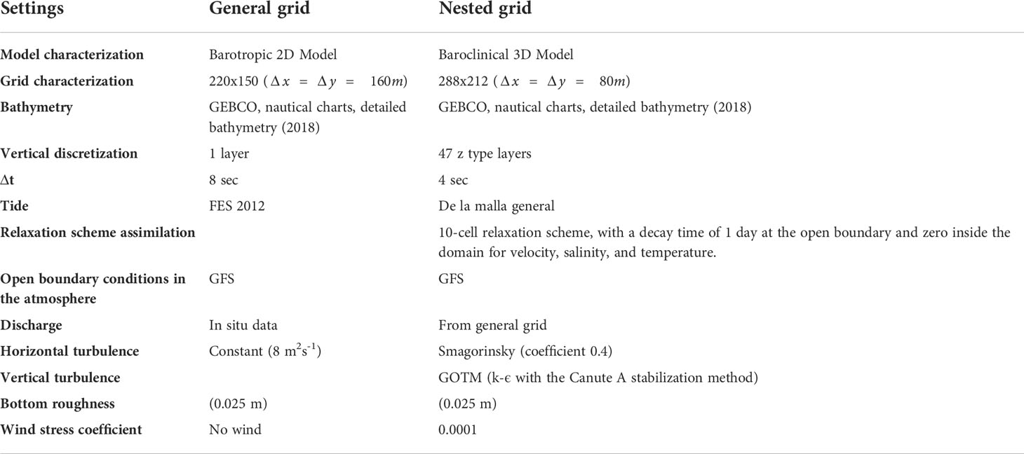
Table 1 MOHID Model configuration.

The general grid provides the open boundary conditions to the detailed grid, which covers an area of 387 km2 with 288x212 nodes, of an 80m cell size, with a time step of 4 s. The nested grid was executed with 35, 40, and 47 vertical z-type layers, showing the best results in the structure of the salinity and density distribution. The modeling began, with a sigma-type vertical discretization in the detail mesh. However, with this configuration, the model underestimates the entry of the saline wedge and presents difficulty in representing the velocity fields at the mouth, due to the strong gradients in the bathymetry in this area.

The transition of hydrodynamic conditions at the boundary of the nested model was performed using a Flather-type relaxation method for barotropic flow, with a relaxation scheme for the velocity, salinity, and temperature fields, spanning 10 cells, with a decay time of 86400 s at the open boundary, and 0 s in the interior of the domain. The Smagorinsky horizontal turbulence closure model was used, whereas the vertical turbulence was solved with the general ocean turbulence model (GOTM); using the k-ϵ vertical turbulence closure model and the Canuto A stabilization method (Canuto et al., 2001). Global Forecast System (GFS) wind data from the node closest to the seaward boundary (11.10’0.048” N, 74°50’0.168” W) was used. Winds were considered constant in space, and variable in time (Δt=3h). The wind stress parameter was calibrated at 0.0001, which presented the best result in the calibration processes on the distribution of salinity and density in the outer delta zone.

On the other hand, the SWAN wave spectral model was run only on the detail grid, using as boundary conditions the WAVEWATCH III (WWIII) and wind (GFS) model wave reanalysis series for the two-case study. The processes of refraction, diffraction, bottom friction, nonlinear wave-wave interactions (quadruplet and triad), wave-current interaction, and dissipation by breakage were considered. The model SWAN provides significant wave height, wave period, wavelength, wave direction, wave-induced force (2D radiation stress), and maximal orbital velocity near the bottom for the hydrodynamical model MOHID 3D.

Bathymetry

The bathymetric information for the construction of the calculation grids was obtained from the GEBCO global database of bathymetry, from official local nautical chart bathymetry and inside the estuary (from the mouth to 40 km inside the river). They used a detailed bathymetry survey in 2018, with multibeam technology and 1m resolution.

Field data

The vertical salinity and density profiles, measured with a Castway CTD, with a sampling frequency of 4Hz, were used to calibrate and validate the MOHID 3D numerical model. The measurements were performed during the dry season of 2018 (Feb 28- Mar 5) and 2020 (Mar 14 and 15). In the 2018 dry season, measurements were made in the outer estuary area, along three transects in a north-west, north, and north-east direction (Figure 1). In addition, profiles were measured, from the mouth-upstream, along two parallel longitudinal transects up to 6 km upstream of the mouth. The exact dates of measurement in each zone, the number of surveyed profiles, and the simultaneously measured river flows are presented in Table 2. During the 2020 low flow season, measurements were taken at two cross sections located in the inner estuary at 2.5 km (S1) and 3.5 km (S2), during one tidal cycle (25 hours), as shown in Figure 1.

TABLE 2

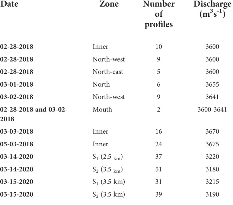
Table 2 Location of salinity profiles, temperature, density, and flow values measured for the 2018 and 2020 dry seasons.

Flows in the estuary during the 2018 dry season ranged from 3600 to 3670 m3s-1, while the 2020 dry season presented an average flow of 3200 m3s-1, according to gauging measurements made in situ with an acoustic Doppler current profiler (ADCP RiverPro). These measurements are considered representative of low flow periods.

Two tide records were made using a pressure sensor (TR 1060 RBR), at points P2 and P3 (Figure 1), located 4 km (11° 04’ 39.48” N, 74° 50’ 43.86” W) and 7 kms (11° 2’ 48.24” N, 74° 49’ 46.74” W) from the mouth of the river. At P3, measurements were taken between February 24 to March 18, 2018, and, at P2, between March 14 and 18, 2018. At point P2, velocity profiles were also measured with a Nortek Aquadopp Profiler current meter, taking data every 10 mins, for 1 min, at a frequency of 1 Hz. The equipment was located at the bottom, at a depth of 10 m, the transducer was installed at 0.7 m from the bottom, with a 0.5 m blanking distance, and a cell size of 0.5 m.

To perform wave measurements was not possible during the field campaigns due to the high energy maritime weather in the months of February and March, which prevented, on both occasions, the installation of wave sensors. Therefore, a third period, from 19-12-2014 to 24-01-2015, was used to calibrate the SWAN model, which has this waves information at point P1 in Figure 1 (11°5’ 55.19” N-74°53’ 17.47 “W). These measurements were made with a 400 kHz ADCP Aquadopp profiler. Burst measurements of 2048 data were taken every hour, at a frequency of 2 Hz. Significant height (Hs), peak period (Tp), and peak direction (Dp) were calculated with the data of each sea state.

Stratification parameters

To analyze the effect of waves on stratification in the MRE, the gradient Richardson number $\left(R_{ig}=\frac{N^2}{S^2}\right)$ was used, where $N^2=\frac{-g}{{\rho }_0}\frac{\partial \rho }{\partial z}$ is the buoyancy term, and $S^2=\left[{\left(\frac{\partial u}{\partial z}\right)}^2+{\left(\frac{\partial v}{\partial z}\right)}^2\right]$ is the shear stress term, Water density and vertically averaged density ρ and ρ₀ (kgm-3), u and v are the flow velocity components (ms-1), z is the depth (m) and g is gravity acceleration (ms-2). To calculate the gradient Richardson number, the velocity (u and v) and density profiles of the model were used. The gradient Richardson number for each profile cell i was determined from the expression $\Delta R_{zi}=\left(\frac{-g}{{\rho }_0}\right)\left(\frac{\Delta {\rho }_i\Delta z}{{\left(\Delta u_{zi}\right)}^2+{\left(\Delta v_{zi}\right)}^2}\right)$. The representative Richardson number of a vertical profile is the median of ΔR_zi (Simanjuntak et al., 2016).

This non-dimensional parameter was used to assess the stability in the water column, and to estimate the mixing rate through the halocline (Dyer, 1991). A Richardson number Rig_c = 0.25 (or normalizing $lo{g}_{10}\left(\frac{R_{ig}}{R_{igc}}\right)>0$) is taken as critical value. Below this threshold the water column is unstable and well mixed (Geyer and Smith, 1987).

Additionally, to quantitatify stratification in the estuary, the potential energy anomaly (ϕ ) (Simpson, 1981; Pu et al., 2016), was used. This parameter represents the amount of work required to vertically mix a unit volume of estuarine water. The potential energy anomaly is defined as $\varphi =\frac{1}{h}\underset{-h}{\overset{0}{\int }}\left(\overline{\rho }-\rho \right)gzdz$, where ρ is the density of estuarine water, and $\overline{\rho }$ is the average density given by the expression $\overline{\rho }=\frac{1}{h}\underset{-h}{\overset{0}{\int }}\rho dz$. When ϕ tends to zero, it indicates mixing, positive values indicate stable stratification, and negative values indicate unstable stratification.

In addition to the stratification parameters mentioned, the Simpson dimensionless number (Simpson et al., 1990) was used. The Simpson number (Si) evaluates the balance between the contribution of the longitudinal density gradient as a driver of circulation and stratification versus the input of the bottom friction velocity as a mixing force in estuaries (Meyers et al., 2015). To evaluate the effect of waves on stratification, the bottom friction velocity scale was modified (U*² =$\frac{{\tau }_{bed}}{\overline{\rho }})$, where τ_bed is the bed shear stress considering the tide, and tidal effects with the waves. The Si number was calculated with the expression ($Si=\frac{H^2}{U{*}^2}\frac{g}{{\rho }_0}\frac{\partial \rho }{\partial x}$), where H is the depth, U*² is the square bottom shear velocity and $\frac{g}{{\rho }_0}\frac{\partial \rho }{\partial x}$ is the longitudinal buoyancy gradient. When Si>1 the system is stratified, for values much higher than 1 it is highly stratified, while for small values (close to zero) the mixing destroys the stratification, and the water column is mixed.

Skills for verification

To show the model’s ability to represent tidal dynamics, currents, and salinity and density gradients in the MRE, during the low flow season, its results, with and without wave effects, were compared to data from field observations. In total, during calibration, measured and simulated levels at points P2 and P3 (Figure 1), the temporal evolution of the velocity profile at point P3, and salinity and temperature profiles measured during the dry season of 2018 were compared. Moreover, for validation, the model results were compared with the distribution of salinity and density, measured during a tidal cycle in the dry season of 2020, in cross sections S1 and S2, as shown in Figure 1.

To evaluate the model, the basic metric statistical indicators root means square deviation (RMSD), Bias, Skill, and Willmot’s coefficient (WS) (Willmott, 1981; Goudsmit et al., 2002) were used.

$RMSD=\sqrt{\frac{1}{N}\left(\sum _1^N{\left(h_{obs}-h_{model}\right)}^2\right)}$

$BIAS=\frac{1}{N}\left(\sum _1^N\left(h_{model}-h_{obs}\right)\right)$

$SKILL=1-\frac{{\sum }_1^N{\left(h_{model}-h_{obs}\right)}^2}{{\sum }_1^N\left|h_{model}-{\overline{h}}_{obs}\right|\left|h_{obs}-{\overline{h}}_{model}\right|}$

$$WS=1-\left(\frac{{\left(\overline{h_{model}-h_{obs}}\right)}^2}{{\left(\overline{\left(\left|h_{obs}-\overline{h_{model}}\right|+\left|h_{obs}-\overline{h_{obs}}\right|\right)}\right)}^2}\right)$$

Where, h_obs and h_model denote time series of observed and modeled data, respectively. For the case of vertical profiles of salinity and density, these statistical indicators were calculated by averaging the measured data every 0.5 m in the water column to match the measured and modeled data (∆z=0.5m , for the model within the estuary). Perfect agreement between the model results and observations yields a SKILL or WS of 1.0, whereas complete disagreement yields a value of 0. While RMSD or BIAS of 0 indicates perfect agreement between the model results and observations yields, and great values indicate complete disagreement yields

Results

This section presents the results of the calibration of the MOHID 3D-SWAN models and evaluates the effects of the (low flow season) waves on: (i) hydrodynamics; (ii) stratification patterns and distribution in salinity; and (iii) dynamics in salt wedge intrusion and changes in the salt front.

Model verification

The comparison between simulated and measured data from water level, velocity, salinity, density and wave parameters it was used: skill, Willmott score, bias and root mean square deviation.

Water velocity and level

Figure 2A shows the measured and simulated vertically averaged velocity at P2. Both series produced: skill=0.82, RMSD=0.0034ms-1, bias=0.0085ms-1, and WS=0.7568. From the value of skill and WS, the ability of the model to represent the velocity in the estuary is observed. In Figures 2B, C, the level comparisons for P2 and P3, respectively, are shown. The model was able to represent level variations along the river channel, including neap and spring tide conditions (Figure 2C) with 0.94 < skill < 0.97 and 0.91 < WS < 0.96, respectively, RMSD and bias minor to 0.01m.

FIGURE 2

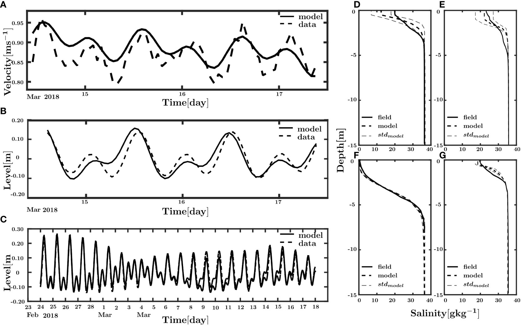
Figure 2 Measured and simulated time series of (A) velocity at point P2. (B) Water level series at point P2. (C) Water level series at point P3. (Including spring and tidal conditions). Comparison of salinity profiles considering wave-current interaction at the. (D) North-west (02-28-2018). (E) North-east (02-28-2018). (F) Mouth (02-28-2018 and 02-03-2018), and (G) North (03-01-2018) zones of the plume.

Salinity and density

Figure 3 shows the measured and simulated mean salinity profile, with the standard deviation of the set of simulated profiles at different locations in the outer zone and at the mouth of the estuary. The model, in this case, includes the effects of waves. A good representation of the vertical distribution of salinity in the area is observed. Table 3 shows the statistical indicators between measured and simulated profiles, with and without wave effects. There, skill values between 0.73 and 0.80 are detected for the simulation with waves, and values between 0.62 and 0.75 for the cases in which the effect of waves is not included in the outer zone. In the mouth, the skill and Wilmott Score present values higher than 0.9 for both cases. These results indicate that the model better represents the salinity gradients in the outer zone of the MRE when the effects of waves are considered.

FIGURE 3

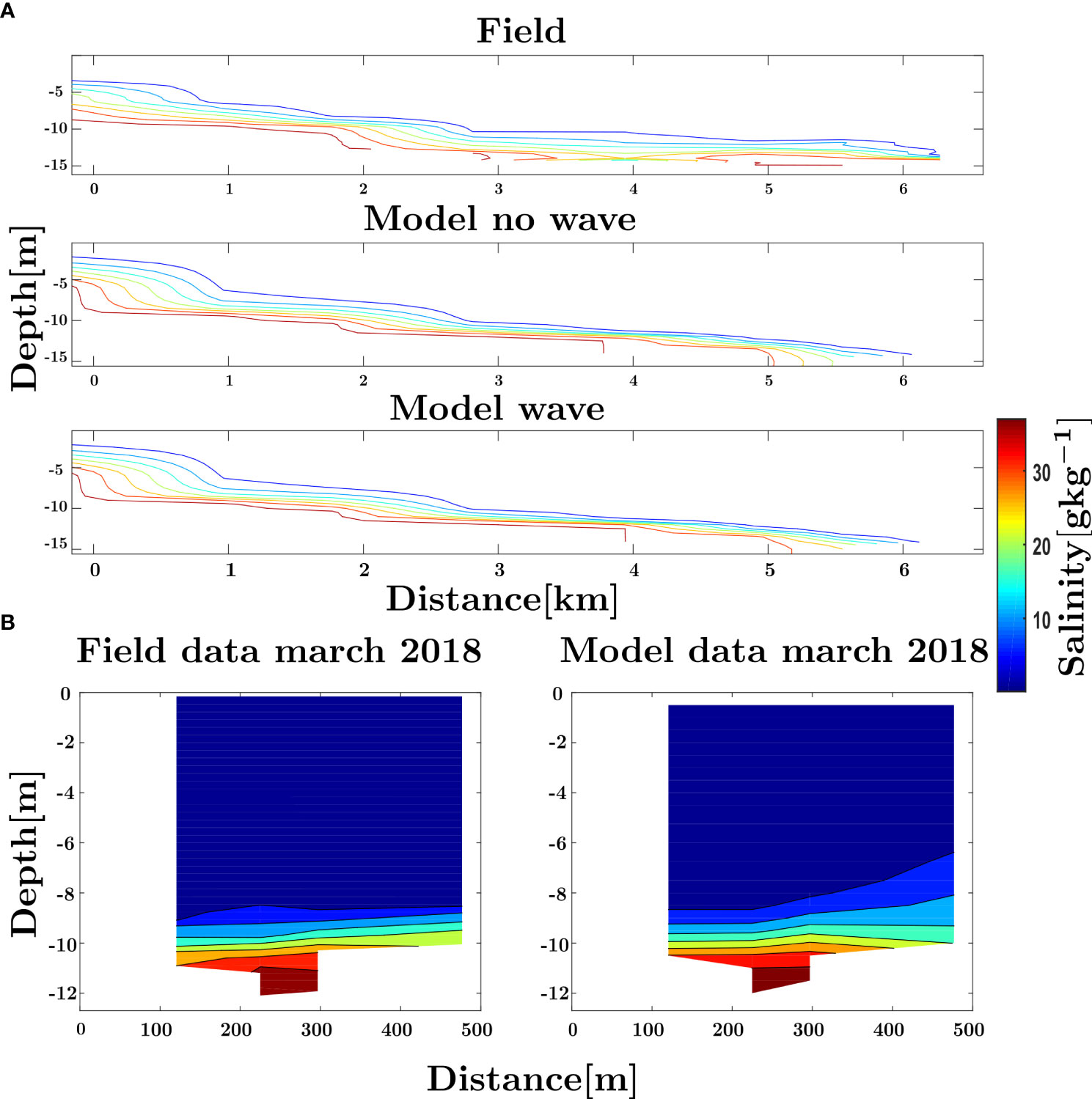
Figure 3 Measured and modeled salinity transects in the inner estuary in March 2018. (A) Longitudinal transect. (B) Transversal transect at km 2 inside the estuary.

TABLE 3

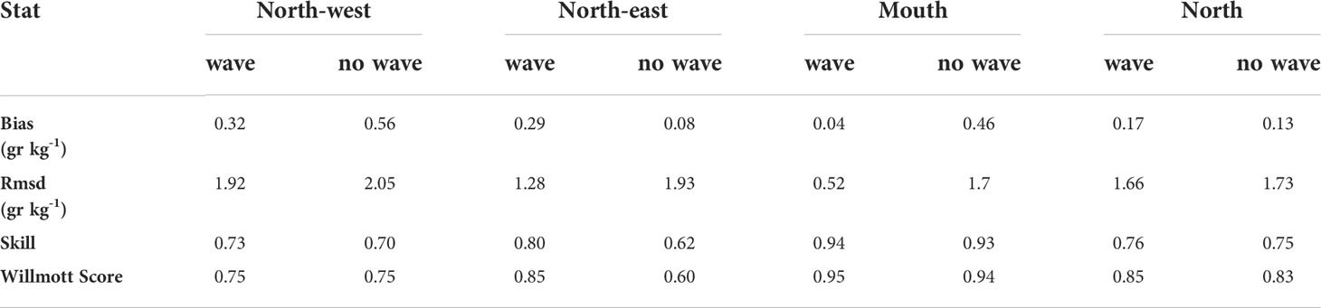
Table 3 Mean statistical indicators for salinity, with and without waves, in the outer zone and at the mouth of the MRE.

Figure 3A shows a longitudinal section in the MRE where the measured and modeled salinity gradients, with and without waves, during the dry season of 2018, are compared. Similarly, the cross-sectional distribution of measured and modeled salinity in a section of the MRE is presented (Figure 3B). The model capably reproduces the strong longitudinal and transverse salinity gradients within the estuary, underestimating the wedge inflow by approximately 400m, with respect to the longitudinal section measurements in March 2018 (Figure 3A).

Model validation with respect to salinity and density distribution was performed with profiles measured during the 2020 dry season. Figure 4 presents the cross-sectional distribution of measured (Figures 4D, F) and simulated (Figures 4E, G) density in sections S1 and S2, respectively (Figure 1). The modeled tidal conditions during the measurement (Figure 4A), and the measured and simulated mean profile with the standard deviation of the simulated profiles (Figures 4B, C) in sections S1 and S2. The model represents the strong gradients in density, and its variability throughout the tidal cycle for this area.

FIGURE 4

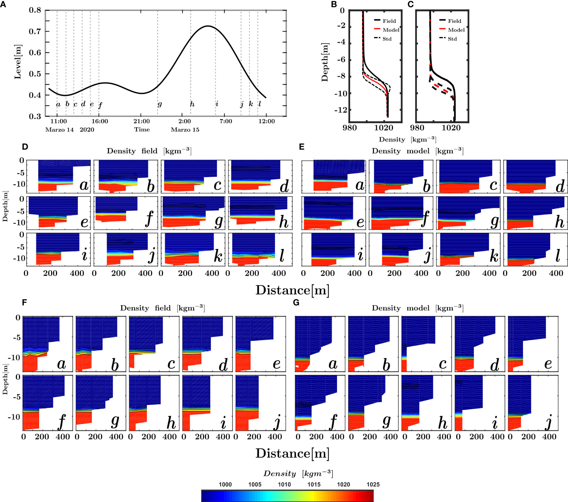
Figure 4 Cross-sectional distribution of measured and modeled density in the inner MRE in section S1 and S2 for the 2020 dry season. (A) Water level.Measured and modeled average density profile S1 (B) and S2 (C). Measured (D, F) and modeled (E, G) density in the cross sections at different tidal stages [according to panel (A)] in sections S1 (D, E) and S2 (F, G). The letters a-l is diferents moments of tide.

Wave

To calibrate the SWAN model, wave data, measured at point P1 at coordinates 11°5’ 55.19” N-74°53’17.47 “W (Figure 1), was used for the 19-12-2014 to 24-01-2015 period (dry season). The Hs and Tp data, measured for the period January 1-15, 2015, were compared with the SWAN model results, as shown in Figures 5A, B). In this area, the SWAN model was able to represent the significant heights with a skill of 0.84, and the peak periods with a skill of 0.8. Then, the SWAN model was run, with the same configuration, to obtain the wave fields in the dry seasons of 2018 and 2020.

FIGURE 5

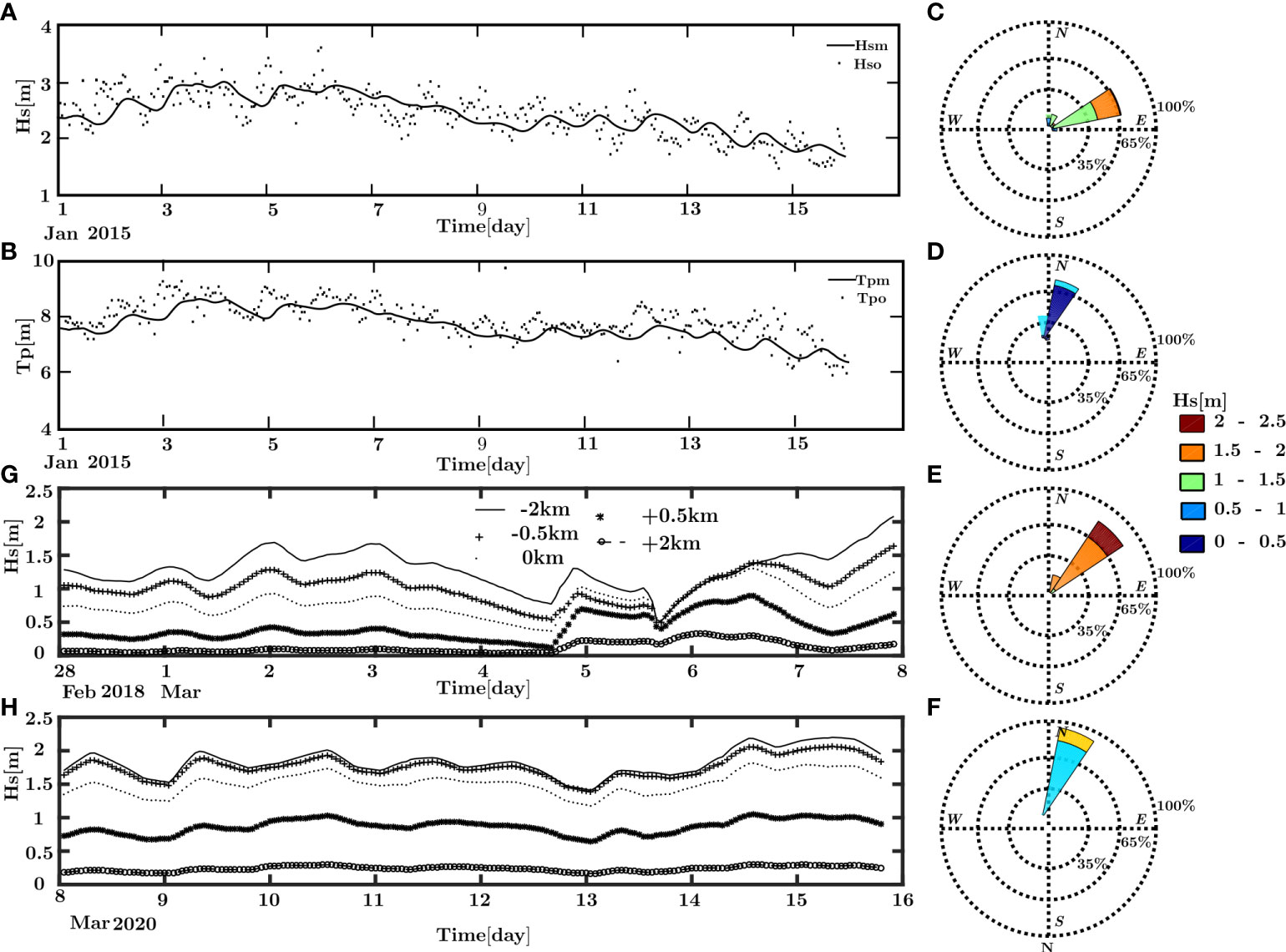
Figure 5 Comparison of measured [(A) Hs and (B)Tp], and SWAN modeled wave parameters in the MRE plume (P1), (skill of 0.83 and 0.80 for Hs and Tp, respectively, were found). Waves rose from SWAN model results at -2 km (outer zone) in 2018 (C) and 2020 (E), and 0.5 km (inner zone), in, (D) 2018 and (F) 2020. Significant wave heights are expected in (G) 2018 and (H) 2020 at various locations.

In Figures 5C–F, simulated wave roses are presented for the 2018 and 2020 dry season at two points, outer zone at -2 km (Figures 5C, E), and inner zone at 0.5 km (Figures 5F, G). In addition, the evolution of the significant wave height around the mouth (-2km, -0.5 km, 0 km, 0.5 km, and 2 km) for the modeled period, 2018 (Figure 5G) and 2020 (Figure 5H), is shown. The wave direction in the outer zone is ENE and NE, with significant wave heights between 1-2 m and 2-2.5 m for the low flow seasons of 2018 and 2020, respectively. This direction is changing due to refraction processes, so that, at the mouth and inside the estuary, the wave direction is N. An energetic wave is observed in the outer zone of the estuary, with significant wave heights between 1.5 and 3.0 m. At the mouth, values between 0.5 and 1.7 m are presented, which decrease in the interior of the estuary (+0.5 km), taking values between 0.3 and 1.0 m. The model shows significant heights between 0.1 and 0.15 m, at 2 km inside the estuary, where most of the wave energy has been dissipated (about 95%). Between March 5 and 6, there was a ground waves with periods between 15 and 17 s, coming from the east, with Hs between 1 and 1.5 m. This wave-type wave presented greater amplification in the mouth zone (Figure 5G).

Effects of waves on hydrodynamics

Figure 6 shows the differences between the average level over the tidal cycle, with and without wave effects, for 2018 and 2020, both in plan and in a longitudinal section along the MRE deep channel. Particularly, in Figures 6A, C, the waves increase the sea level in the area east of the mouth, with level variations between 0.04 and 0.06 m for 2018, and between 0.06 and 0.09m for 2020. This is due to the contribution of the waves in the sea level variations in the breaker zone (setup) of the beach located east of the mouth. In the frontal zone (low subtidal), level increases are observed, with a maximum of 0.02 in 2018 and 2020, meanwhile, between the mouth and 0.5 km, the waves produce the tendency to increase the level, as shown in Figures 6B, D, with percentage differences in level, positive for both cases, between 1 and 4% for 2018 and 2020. From 0.5 km upstream, negative percentage differences (between 0 and -1%) are presented for both cases (2018 and 2020), with a small level increase of less than 1% between 1.5 and 2 km, for the 2020 dry season (Figure 6D).

FIGURE 6

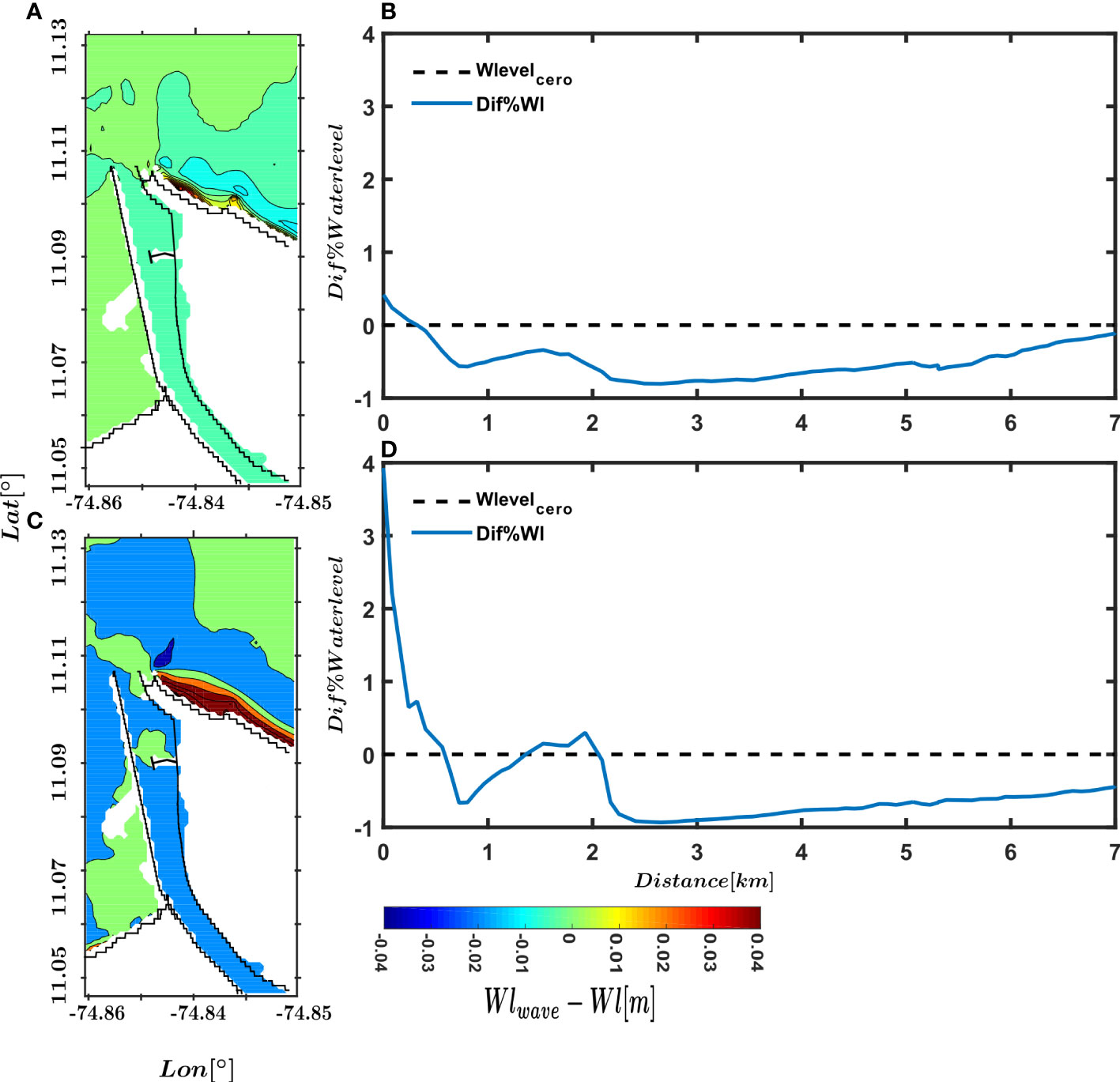
Figure 6 Difference of water level averaged in tidal cycle with and without waves effects for (A) 2018 and (C) 2020. Percentage difference of water level averaged in tidal cycle with and without the effects of waves in a. Longitudinal section in (B) 2018 and (D) 2020.

In Figures 7A, C, the difference in the velocity distribution of the component parallel to the channel (V) is presented, in addition to the vector difference of the components (U_w−U,V_w−V ) with and without waves, showing the difference of the river flow with black vectors and the flow of the salt wedge with red vectors. A decrease in velocity is observed when the effects of waves on hydrodynamics are considered in most of the longitudinal section, presenting differences in the upper mouth (river) zone of up to -0.02 and -0.03 ms-1 for 2018 and 2020, respectively. In the salt wedge zone, maximum differences of 0.02 and 0.04 ms-1 are presented for 2018 and 2020, respectively. Then, the waves weakened the river velocity and the inlet velocity of the salt wedge in both seasons. In 2018, the decrease of the velocity component parallel to the channel was more relevant around the mixing zone between the mouth and km 7, whereas, in 2020, the velocity decrease was more significant between the mouth and km 2 for the river and salt wedge flow.

FIGURE 7

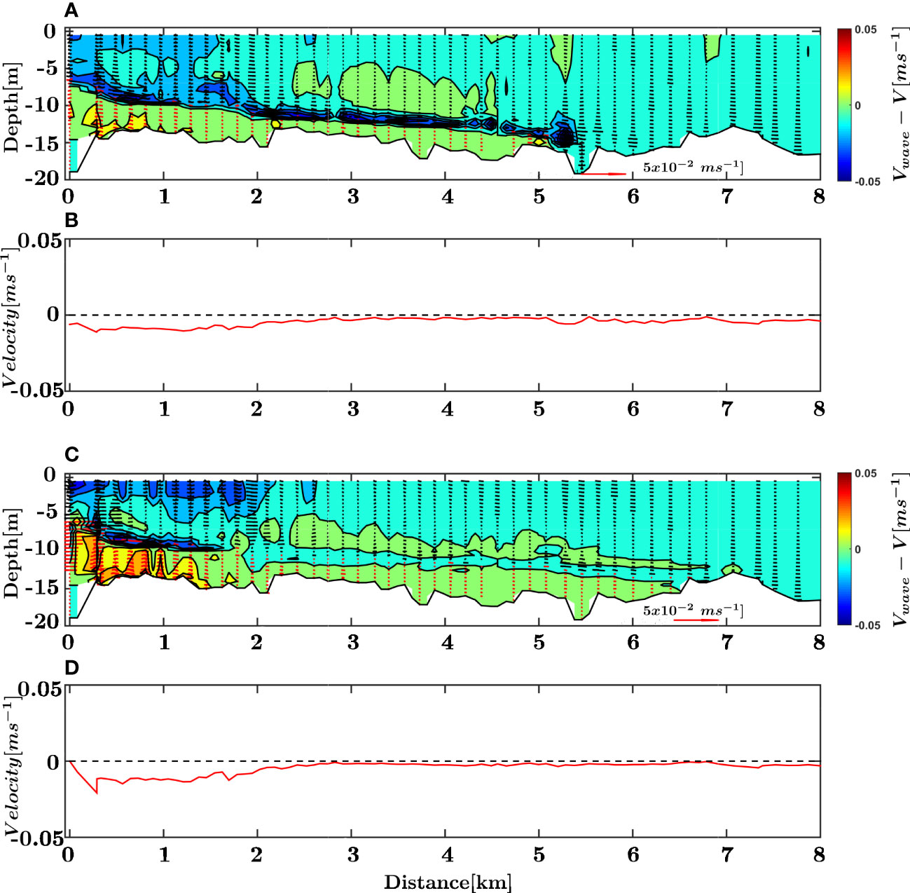
Figure 7 Difference in longitudinal velocity distribution, with and without waves, averaged over a spring tidal cycle: (A) Dry season, 2018 and (C) Dry season, 2020. (Black and red vectors indicate the difference in river and salt wedge velocity, respectively). Differences in vertically averaged velocity along the estuary for the (B) Dry season, 2018 and (D) Dry season, 2020. (Flow to the sea is considered positive, while flow to the river is considered negative).

Figure 8 presents the differences in velocity, with and without waves at the surface, at the bottom and vertically averaged, in the spring tidal cycle, for 2018 and 2020. The largest differences in surface (Figures 8A, D) and vertically averaged (Figures 8C, F) velocity were presented in the north-east area, due to the waves break, which generates increases in the littoral currents, with variations of up to 0.1 and 0. 15 ms-1, for 2018 and 2020, respectively. The largest differences in bottom velocity (Figures 8B, E) occurred in the frontal zone of the mouth (subtidal flats) and in the north-eastern zone, adjacent to the mouth, with differences of up to -0.05 and -0.1 ms-1 for 2018 and 2020, respectively. In the inland zone, the greatest wave effects on velocity occurred between the mouth and km 2, with differences in surface velocity of up to -0.01 and -0.02ms-1 for the 2018 and 2020 dry seasons, respectively, with a greater effect on velocity in the season with the most energetic waves (2020).

FIGURE 8

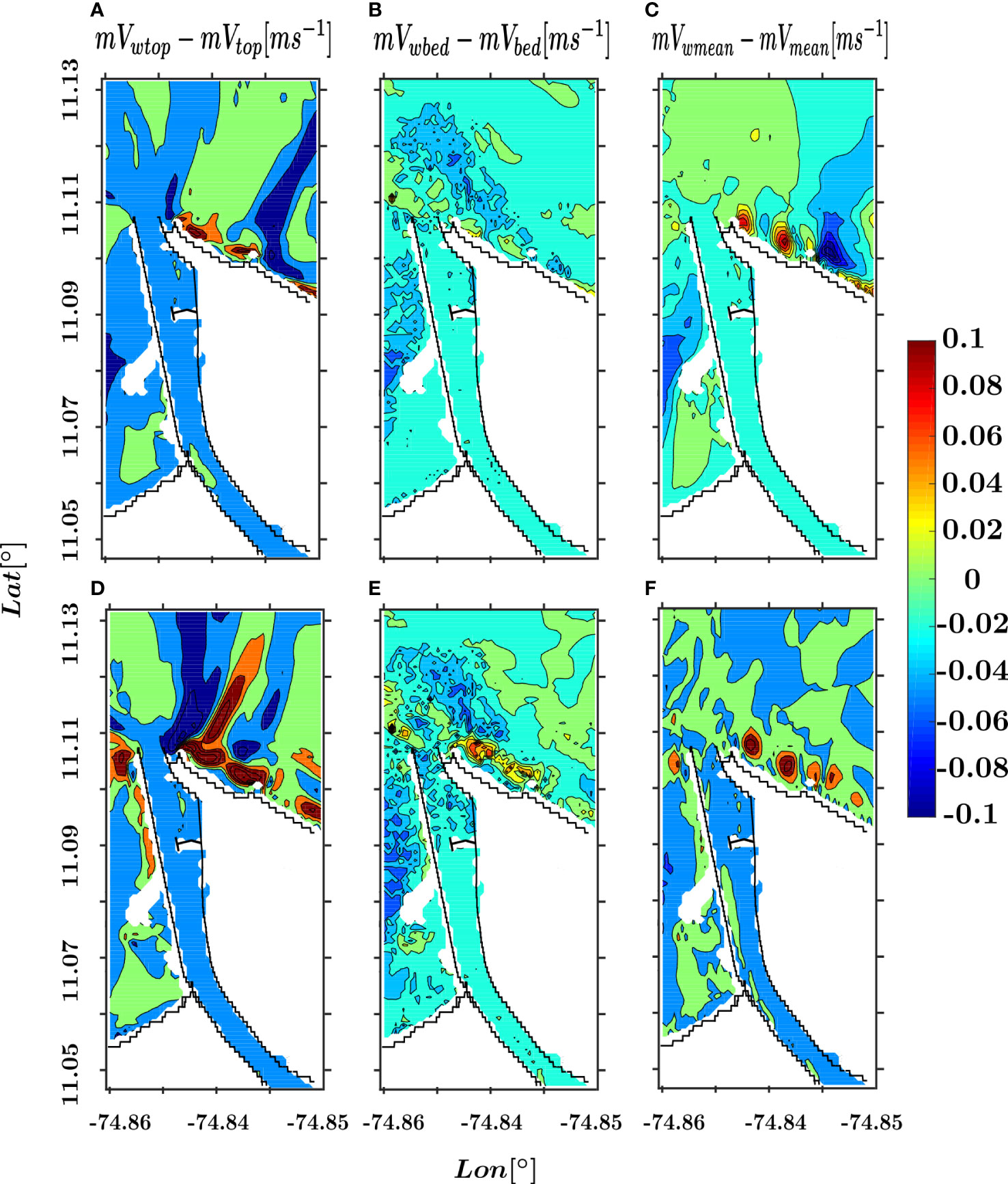
Figure 8 Differences in tidally averaged velocity magnitude, with and without waves at the surface (A, D). Bottom (B, E), and vertically averaged (C, F), in 2018 (A–C), and 2020 (D–F).

Wave effects on intrusion and the saline front

Figures 9A, B shows the length of the saline intrusion with the effect of the wave (red) and without the wave (black), for the dry seasons of 2018 and 2020. Figures 9C, D shows the level and mean value of salinity at the saline front boundary without the effects of waves for the 2018 and 2020 dry seasons, Figures 9E, F shows the level and mean value of salinity respectively at the saline front boundary with the effects of waves for the 2018 and 2020 dry seasons, and Figures 9G, H) shows averaged frequency buoyancy in the front salt wedge with and without effects of waves for the 2018 and 2020 dry seasons. According to the Figure 9, the salt wedge penetrations for the 2018 modeling period were between 5300 and 6150 m, with and without wave effects, presenting a maximum instantaneous difference in the salt intrusion of 100 m (Figure 9A), while, for the 2020 modeled modeling period, the salt intrusion with wave effects varied between 6900 and 7250m and between 7000 and 7300 m, without wave effects, presenting a maximum instantaneous difference of 160 m (Figure 10B). The greatest penetration into the salt wedge occurred when the model did not account for the effects of wave-current interaction for the two modeled cases, but with instantaneous variations of less than 2%. These small differences in salt intrusion, with and without wave effects, show that waves are not a relevant factor in salt wedge variations, whereas the diurnal tidal cycle generates changes in intrusion up to 850 and 920 m, for 2018 and 2020, respectively. These variations are more relevant in spring tidal conditions. In addition, the inflow and retreat of the salt wedge are independent of wave effects, being mainly affected by the diurnal tidal cycle (Figures 9C, D), presenting the greatest variation in the length of the salt wedge (of 1200 and 1100 m) in spring tide for 2018 and 2020, respectively. In neap tide conditions (2018), similar values are observed in the length of salt wedge intrusion for 2018. In high tide conditions (at spring tide), a decrease in the magnitude of salinity is observed in the salt front, taking average values between 10 and 20 for both seasons, with and without wave effects; Considering that, for low tidal amplitudes, there are higher mean salinity values between 25 and 32, showing that the increase in mixing in the water column induced by high tide a decrease in salinity and the frequency of buoyancy in the front salt wedge and low tide favors baroclinic circulation is more effective, increasing salinity and buoyancy frequency in the saline front (Figures 9C–H).

FIGURE 9

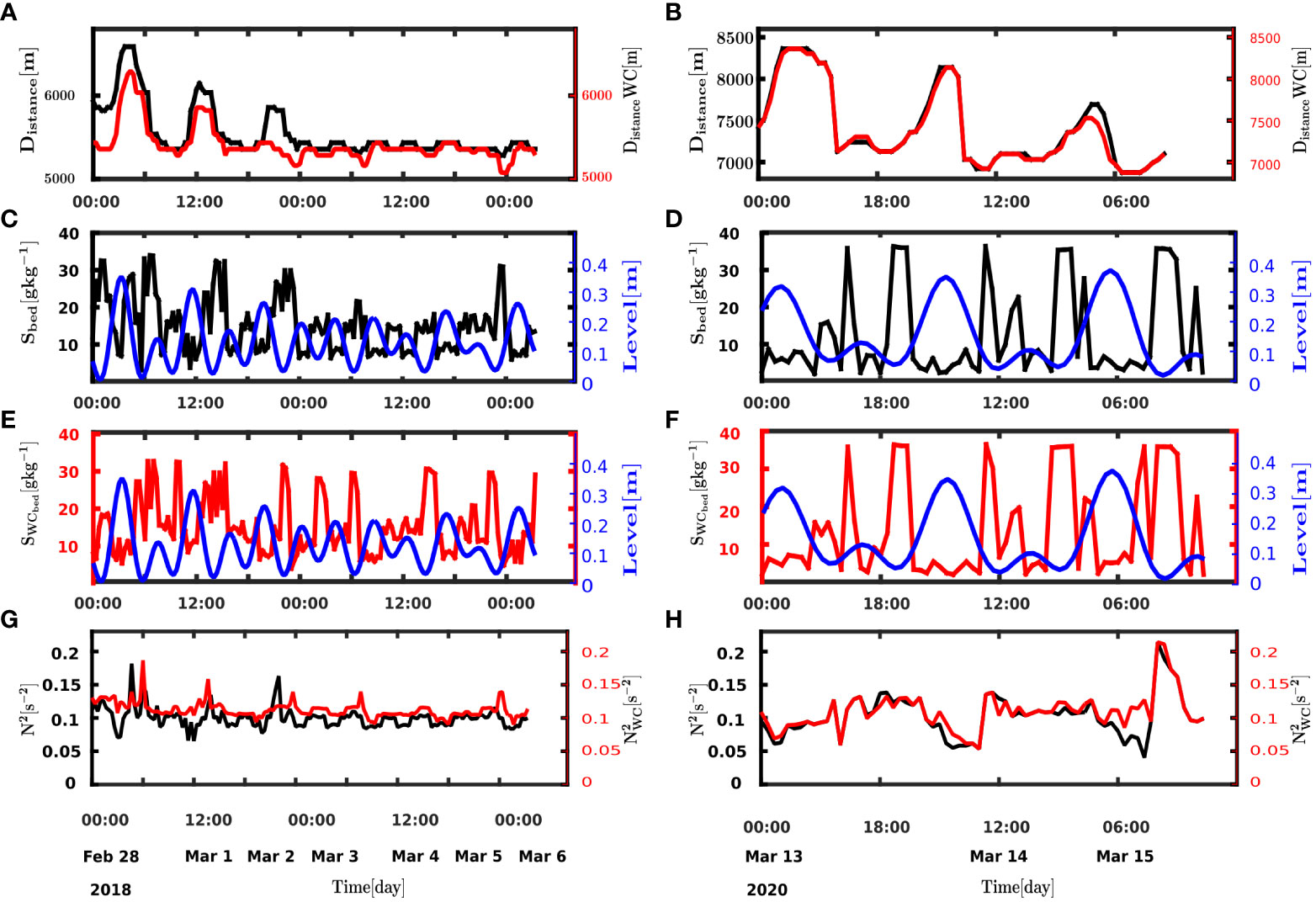
Figure 9 Temporal variation in saline intrusion length the dry season 2018 (A) and 2020 (B) with (red) and without (black) wave interaction. Water level and mean salinity at the salt front (averaged over the last 200 m of the salt wedge, with the salt wedge boundary set at 2 gkg-1) without wave interaction for the 2018 dry season (C) and the 2020 dry season (D) and with wave interaction 2018 dry season (E), and 2020 dry season (F). Averaged buoyancy frequency at the salt front the 2018 dry season (G) and the 2020 dry season (H).

FIGURE 10

Figure 10 Gradient Richardson number normalized for the dry season 2018 (A) and 2020 (E). Simpsons number averaged over the spring tidal cycle for the dry season of 2018 (B) and 2020 (F), potential energy anomaly averaged over the spring tidal cycle for 2018 dry season (C) and 2020 (G). (Without waves in black and with waves in red). and bottom shear velocity averaged over the spring tidal cycle for 2018 dry season (D) and 2020 (H).

Vertical mixing and layer processes

Figure 10 depicts the normalized gradient Richardson number (Figures 10A, E), dimensionless Simpsons number averaged over the spring tidal cycle (Figures 10B, F), potential anomaly energy for a longitudinal section averaged over the spring tidal cycle (Figures 10C, G), and bottom shear velocity averaged over the spring tidal cycle (Figures 10D, H), calculated with the model for the 2018 dry season (Figures 13A, B), and 2020 (Figures 10C, D), calculated with the model data, with and without wave effects. Values greater than zero are observed for the normalized gradient Richardson number, dimensionless Simpsons number and for the potential energy anomaly, which is related to the stratification generated by the presence of the salt wedge in both seasons. Between the mouth and the 1st km, there is a 10% decrease in the gradient Richardson number as calculated with the effects of waves, which shows how the waves induce a reduction in the stability of the water column. However, in this same section, there are no significant changes in the potential energy anomaly (percentage differences of less than 2%), so the decrease in the gradient Richardson number may be related to the increase in the total shear stress in the water column, while, when the effects of the waves are considered, between the mouth and 2 km, the Si presented presents a difference, for 2018 and 2020, of -59 and -125%, respectively. At the same way the bottom shear velocity showed differences of 58 and 93%, for 2018 and 2020, respectively. Between 2 km and the highest penetration of the salt wedge, the percentage difference of Si and U* was less than 10 and 30%, respectively for both modeling scenarios.

Between the 1st km and the zone of maximum length of salt intrusion, the gradient Richardson number registered values higher than 0.25, both with and without waves. However, this parameter is higher, between 4% and 10%, when the contribution of waves is not considered for the dry seasons. The potential anomaly energy presented lower values, between 5 and 12% difference, for the data without and with the effects of the waves, indicating that the effect of the waves is manifested in a decrease in the intensity of the stratification.

Figures 8A, C show the difference in salinity distribution, with and without wave effects, averaged over the tidal cycle, for a set of cross sections between the mouth and Km 2, for the 2018 and 2020 dry seasons. Figures 8B, D show the difference in longitudinal salinity distribution averaged over the spring tidal cycle, with and without wave effects, for 2018 and 2020, respectively. For both seasons, percentage differences between -5 and 5% are present, with and without wave effects; these differences are largest around the halocline and mixing layer.

For flow conditions of 3600 m3s-1 and Hs=0.70m at the mouth (2018), an intensification of salinity is observed in the halocline (between 1 and 2.5), which is more significant in the phases of major and minor ebb, while in the rest of the longitudinal section, there is a decrease in salinity between -0.1 and -0.3. There are three clearly distinguishable zones: between the mouth and 320 m, where the waves generate lower average salinities in almost the entire section, except for an increase in salinity on the left bank between 400 and 1000 m towards the interior of the river (Figures 8A, C). A second zone (between km 1 and 2), where the waves weaken the magnitude of salinity between 6 and 10 m depth -0.2 and -0.5 for 2018 and 2020, respectively, which is associated with a decrease in the frequency of buoyancy, produced by changes in velocity due to the narrowing works in this area of the river. A third zone (between km 2 and 7), where higher intensity in salinity prevails without wave effects for 2018 (Figure 8B), and a decrease in salinity for 2020 (Figure 8D. In the halocline zone, a third zone (between km 2 and 7) with higher salinity intensity without wave effects for 2018 (Figure 8B) and a decrease in salinity for 2020 (Figure 8D); these differences are primarily generated in the internal mixing layer for the two modeling scenarios (Figures 8A, C). The flow for 2018 and 2020 was 3600 and 3200 m3s-1, respectively. In the case of lower waves (2018), there was a higher flow, implying higher turbulent kinetic energy in the halocline zone, which added with the mixing produced by the waves induces an increase in salinity between Kms 2 and 7, observing positive differences in salinity (Figure 8B). Meanwhile, in 2020, there was a lower flow and a higher significant wave height, generating a decrease in salinity (km 2 to 7) (Figure 8D). This indicates that even though the difference in flow for the 2018 and 2020 cases is 500 m3s-1, this parameter has a relevant role in evaluating the effect of waves on the distribution of salinity in the halocline zone. For 2018, between km 2 and 4 (Figure 8A), the increase in salinity in this zone may be associated with the greater availability of water, which when mixed generates an increase in salinity due to the extra energy provided by the waves in this part of the mouth; meanwhile, for 2020 (Figure 8C), the excess mixing induced by the waves occurs between km 0 and 1.

Figure 10 show the residual difference of the salinity distribution, with and without waves, for the first 8 layers, between the surface and 3.5 m deep, for 2018 and 2020. In both cases, great variability is observed in the distribution of the differences in salinity, which are more significant between 0 and 2m, which corresponds to the dispersion zone of the river plume. The greatest differences in salinity are found in the northeast zone (differences greater than 1), while in the northwest zone, negative salinity differences were observed in the same layers, showing that the waves advects the river plume towards the northwest, and that the greatest variations in salinity in the outer zone occur mainly around the mixing layer (between 0 and 1. 5m), whereas, in the inner zone, the differences in salinity are not significant in these layers, moving to deeper zones, as observed in the cross-sectional distributions in the interior of the MRE (Figure 11). The greater differences in the north-east zone may be related to the increase in the coastal currents produced by the wave break in this zone, which force the plume to disperse to the north-west, which is where the lowest salinities are present in the modeling, without including the effects of the waves.

FIGURE 11

Figure 11 Differences in the transversal (A, B) and longitudinal (C, D) salinity distribution, with and without waves interaction, averaged over the spring tidal cycle, during the dry season of 2018 (A, C) and 2020 (B, D).

Discussion

The gradient Richardson number, shear stress, buoyancy frequency, and potential energy anomaly are the parameters that were used to understand the wave effects on stratification. The effects of waves on hydrodynamics, salinity distribution, and salt wedge dynamics the differences in velocity, level, and salinity as averaged over the spring tidal cycle, were analyzed

Model verification

This highlights the importance of considering wave dynamics in the analysis of hydrodynamics and stratification in estuarine systems with high wave energy, such as the MRE.

Comparing the modeled salinity profiles, with and without waves, with the measured data (Figures 2D–G) shows a better fit in the salinity distribution in the outer zone when waves are considered (Table 3). This could be because the waves help to represent more realistic conditions in the system (Bakhtiari and Zeinoddini, 2011; Schloen et al., 2017), whereas, in the inner estuarine zone, with and without wave effects, the model represented strong longitudinal and transverse gradients in salinity and density distribution (Figures 3, 5, 6). Furthermore, the wave induces higher salinity in the pycnocline zone (2018), and lower salinity at the bottom (2018 and 2020). In the 2018 dry season, the salt wedge intrusion length calculated by the model was 6100 m, for flow conditions of 3600 m3s-1, wind speeds between 4.5 and 12 ms-1, and significant wave heights of 1. 2 m at the mouth, but for the 2020 dry season, the maximum salt wedge intrusion length was 7300 m, for flow conditions of 3200 m3s-1, wind speeds between 5 and 12 ms-1, and wave conditions of 1.0 m at the mouth of the MRE. The model results show an underestimation in the salt wedge of approximately 300 m for the 2018 dry season, and 500m for the 2020 dry season. This difference in the measured and modeled salt wedge inflow, in the two case studies, may be related to the cell size in the detail grid (∆x=∆y=80m ) and the vertical turbulence closure models (Ralston et al., 2017). Another aspect that affects the dynamics in salt wedge intrusion length are the complex variations in bottom morphology. Given that the bathymetry used to construct the computational grids was performed in 2018, and the system exhibits morphological changes between 2018 and 2020. These intra-annual changes have been reported by Restrepo et al. (2020) and Ávila (2021), who, from the analysis of bathymetric information from the MRE for the 2006-2012 and 2000-2017 periods, respectively, found unstable morphological conditions along the riverbed, high erosion, and sedimentation rates in different areas of the channel. These morphological changes influence the pattern of salt wedges and stratification dynamics (Pu et al., 2016; Jovanovic et al., 2019; Zachopoulos et al., 2020).

When comparing the modeled and measured significant height and peak period data for the January 1 to 15, 2015, period, the SWAN model was able to represent significant heights and peak periods with a skill of 0.84 and 0.8, respectively. These skill values are acceptable for estuarine systems with complex bathymetry such as the MRE (Clunies et al., 2017).

Effects of waves on hydrodynamics

The results show that waves affected the level and current fields in the MRE, this can be observed in: (i) An increase in the level in the area east of the mouth due to wave breaking and in the interior of the estuary (mouth up to km 2) while, for distances greater than 2 km, the interior of the estuary dissipates the effects of the wave on the tide, showing that, in this area, the transition from wave dominance to tidal dominance is present (Davis and Fox, 1981; Dalrymple et al., 1992) (ii) An increase of longitudinal currents induced from waves in the eastern zone of the mouth; in this zone, there is the greatest variation in the magnitude and direction of the currents, due to wave breaking and the increase of shear stress; this increase of the coastal currents can contribute to the deflection of the dispersion of the plume towards the northwest in the mouth zone, (iii) decrease of the velocity in the frontal zone of the mouth and in the interior of the estuary, the salt wedge decreased due to the effect of the waves; this decrease was more significant in the mouth, between 5 and 7m from surface, taking percentage difference values of 8.3 and 6.5% for 2018 and 2020, respectively. In the case of 2018, the differences in velocity extend up to km 7, with negative differences around the halocline (Figure 7A), while, for 2020, the differences are more significant between the mouth and km 2 (Figure 7C); these changes in velocity coincide with the areas where greater variability in the longitudinal distribution of salinity is present (Figure 8). Decreases in flow velocity were reported in systems where the direction of wave and water flow are opposite, and it is more significant in times of low flows (Jia et al, 2015) (iv) decrease in mean velocity in the inlet zone of the salt wedge (between km 2 and 7). These variations, induced by wave effects on hydrodynamics, may affect the stratification process and fine sediment dynamics in the MRE. The greatest effect of wave on hydrodynamics was on the setup in the inner estuary and in the eastern zone, an effect that was reported in different estuarine zones (Olabarrieta et al., 2011; Chen et al., 2019). The wave induces lower velocity in the halocline, which increases mixing and weakens stratification, and the decrease in bottom currents dissipates the salt wedge inflow, which was more relevant in 2020, due to the higher wave energy.

Wave effects on saline intrusion and saline front

The variation of the position of the salt wedge within the microtidal estuarine channel is determined by the balance between the baroclinic pressure gradient due to the longitudinal density difference, the retarding force of the opposite flow velocity of the river (Chanson, 2004; Haralambidou et al., 2010), and the difference in the baroclinic pressure gradients due to the longitudinal density difference and the difference in barotropic gradients. Furthermore, in systems with significant wave energy, strong wave-induced vertical mixing can occur, which can weaken stratification and reduce saline intrusion (Chen et al., 2019).

In the two modeling scenarios, a decrease in salt wedge (Figures 9A, B) was presented when wave effects were activated. This may be related to: (i) wave-induced increase in mixing, as seen in the decrease of the gradient Richardson number (Figures 10A, C), which is accompanied by an increase in shear stress in the pycnocline (Figure 13), between the mouth and km 2. This mixing, produced by the increase in shear stress, induces a decrease in the intensity of salinity, affecting the baroclinic pressure gradient, which decreased between the mouth and km 1, by 7% and 5%, for 2018 and 2020, respectively. (ii)decrease in the vertically averaged velocity between Kms 2 and 7, in the area where saline intrusion occurs (Figures 8C, F). This decrease in velocity occurs in response to the decrease in the baroclinic gradient, generated by the waves between the mouth and Km 2.

The decrease in saline intrusion was recorded in highly stratified estuaries such as the Modaomen estuary (Gong et al., 2018a) and the Pearl River estuary (Gong et al., 2018b), and in partially stratified estuaries such as Chesapeake Bay (Li et al., 2007) and the York River (Gong et al., 2007), under storm-type energetic wave conditions. Within the estuary, the waves induce variations in circulation and stratification patterns, including weakening and strengthening of stratification (Bolaños et al., 2014). In the case of the MRE, it can be seen as a decrease in the potential energy anomaly, a decrease in the gradient Richardson number (Figure 11), and changes in stratification patterns and halocline intensity, as shown in Figure 8 (Gong et al., 2018b).

Variations in the length of salt intrusion in the diurnal cycle and salinity at the salt front under low flow conditions are mainly affected by the tidal signal, which is more significant under spring tidal conditions, whereas, under quadrature tidal conditions, no significant changes in salt wedge inflow were observed (Figure 9).

The changes in the magnitude of salinity at the salt front (Figure 9) may be related to the competition between the level gradient produced by the tide, the opposition by the flow of fresh water, and the frictional processes that the mixing between the river water and the salt wedge generates. In the saline front (Figures 12C–F), gravity-driven flow is limited by bottom friction and discharge. At high tide, the vertical mixing in the water column increases and the baroclinically driven circulation is weak, which explains the decrease in salinity in the salt front, while at low tide, the turbulence in the salt front decreases and the baroclinic circulation is more effective, presenting increases in salinity, which can be verified in the variation of the buoyancy frequency (Figures 9G, H) (Linden and Simpson, 1988, Simpson and Linden, 1989). When comparing the variations of the salt wedge in the diurnal cycle, a variation of 1.0 km, approximately, in the salt wedge under similar flow conditions (Figures 9A, B). The increased salt intrusion in 2020 may be related to a lower flow (Table 2) and a higher tidal amplitude, as observed in Figure 9; showing the importance of the tide in the entry and retreat of the salt wedge in microtidal systems, given that, in low flow conditions, the variability in the salinity of the salt front and the position of the salt wedge is modulated mainly by the tide and is independent of the waves (Perales-Valdivia et al., 2018).

FIGURE 12

Figure 12 Difference in salinity distribution, with and without waves, for the dry seasons 2018 (upper panels) and 2020 (lower panels). Every 0.5m from the surface to 3.5 m depth.

FIGURE 13

Figure 13 Vertical shear stress and buoyancy frequency at the top picnoclyne, middle picnoclyne, and down picnoclyne averaged over a spring tidal cycle, with (red) and without (black) waves, during the dry season of (A) 2018 and (B) 2020.

Effects of waves in the stratification and vertical mixing process

Figure 11 shows the indicators of stratification and vertical mixing inside the estuary. The high values in the gradient Richardson number, the dimensionless Simpsons number and the potential energy anomaly are an indicator of the high stratification in the water column between the mouth and the front of the salt wedge. When comparing these three parameters (Rig, Si and AEp) with and without the effects of the waves, between the mouth and 2 km there is a negative percentage difference, indicating that the waves induce a weakening of the stratification in this area, mainly in the dry season 2020 where the waves were more energetic. This negative percentage variation is more relevant in the Si parameter (Figures 11B, F), in agreement with an increase in the bottom shear velocity (Figures 11D, H).

The high values in the Si parameter are related to an increase in the longitudinal buoyancy gradient, an indicator of the effect of baroclinic forces on the circulation and stratification, and a decrease in the bottom shear velocity, showing that the circulation becomes weaker due to wave-induced mixing, (Zhang et al., 2022). It is observed that the waves induce a decrease in the entry of the salt wedge and the mouth of the river plume between 0-1 km (Figure 7), which was more relevant in 2020; this happens due to the decrease in the longitudinal gradient of density (Figure 11F), produced by the increase in shear velocity (Figure 11E), which shows how the increase in wave mixing generates a decrease in the longitudinal gradient of density. The reduction of the gradient Richardson number when considering the waves, is an indicator of the instability in the water column that can be related to the increase in the bottom shear velocity (Figures 11D, H) and an increase in the shear stress (Figure 12).

When comparing the modeling results with and without the waves, longitudinal and transverse variations in the salinity distribution were observed in the two simulated periods (Figure 8). These variations may be related to the direction in which the wave impinges on the mouth (NNE and N), which induces an increase in the magnitude of the salinity distribution in the western section of the mouth, because the wave incidence affects advective transport, inducing higher salt transport (Figures 8A, C) (Gong et al., 2018a). Between ~400 and 1000m, greater salinity is present in the area surrounding the pycnocline (Figures 8B, D), due to the decrease in the longitudinal component of the velocity in this area. Then, between km 1 and 2, the waves induced a weakening in the magnitude of salinity (Figures 8B, D), produced by the increase of shear stress in this zone. The variations in stratification can be observed when evaluating the buoyancy frequency and shear stress in the presence of waves, above the halocline, in the halocline, and below it (Figure 12), where higher values of shear stress were observed in the halocline and above it (percentage differences between 3 and 6%), decreasing stratification in these layers due to greater mixing, while below the halocline there was a decrease in shear stress (between 4 and 7%), inducing higher values in the buoyancy frequency (stratification indicator) in the layer below the halocline. These changes may be related to the decrease in the baroclinic gradient in this area.

The waves affect the intensity of the halocline, showing a variation in the difference in positive salinity (∆s=s_wc−s ) between the mouth and the first kilometer; negative, between kms 1 and 2; meanwhile, from the second kilometer to the zone of greater entry of the salt wedge, ∆s>0 can be observed for 2018, related to the decrease in velocity near the halocline and the greater availability of water to be mixed with the excess of energy produced by the waves. For 2020, ∆s<0 , related to the higher mixing produced by the more energetic waves. In both cases, the variations in the distribution of salinity are between ±5%.

Conclusion

The coupling between the MOHID 3D water body hydrodynamic model and the SWAN spectral wave model was applied to evaluate the effects of waves on circulation, stratification processes, and salt wedge dynamics in the microtidal wave dominated MRE under low freshwater discharge conditions, when the estuary exhibits salt wedge behavior. The model was calibrated and validated with observed data from 2018 and 2020, respectively. The coupled model was able to represent the strong vertical gradients in salinity and density in the inner and outer estuaries, as well as the spatio-temporal variations in water level and velocity.

The results show that under low river flow conditions the waves can generate:

● Water level rises at the mouth, as well as the north and northeast delta fronts.

● Changes in circulation patterns in the outer zone of the estuary and decrease in level after 2 km outside the estuary.

● Reduction of current velocity between the mouth and 2 km upstream. This reduction occurred in the river outflow and in the salt-wedge inflow. In the low flow season of 2018, the decrease in velocity extended to the zone of higher salt wedge inflow, which is more intense above and below the halocline.

● Changes in the longitudinal and transverse distribution of salinity and density. The waves affect stratification differentially along the estuary, generating more mixing between the mouth and 0.5 km seaward. Localized increases in salinity are observed in this sector on the left margin and in the halocline.

● Increase and reduction of salinity and density in different zones inside the estuary with more significant effects between the mouth and 2 km inside the estuary. Here the waves induce a weakening in the stratification due to the increase in mixing produced by the bottom shear velocity.

● Changes in the dispersion and stratification of the river plume. Waves favor defection of the plume to the northwest, generating a decrease in salinity in this zone and an increase in salinity in the northwest. These changes in the dispersion of the plume are more significant between the surface and 1.5 m depth.

● Changes in the front salt wedge, at high tide, the vertical mixing in the water column increases and the baroclinically driven circulation is weak, which explains the decrease in salinity in the salt front, while at low tide, the turbulence in the salt front decreases and the baroclinic circulation is more effective, presenting increases in salinity.

● There was a decrease in the salt-wedge intrusion between 180 m and 320 m in the evaluated scenarios. This reduction may be related to changes in stratification and a decrease in the speed of propagation of the salt wedge into the salt front.

In general, the results of this research show that, under low river flow conditions, the tide and waves are key forces in the variation of circulation, stratification, and behavior of the salt front. This work contributed some significant elements to the understanding of the effects of waves on the hydrodynamics of strongly stratified and wave-energetic estuaries.

Data availability statement

The raw data supporting the conclusions of this article will be made available by the authors, without undue reservation.

Author contributions

AHÁ have include calibration and validation of the numerical model, acquisition of field data, analysis of data, writing of the paper. LO and JR were the supervisors and contributed to conceiving the topic and the development of the argument, interpretation of the results, and writing. OÁ contributed to the interpretation of the results and writing. All authors contributed to the article and approved the submitted version.

Funding

This research was funded by Colciencias (Departamento Administrativo de Ciencia, Tecnología e Innovación), National Doctorates Program 727-2016, and the DIDI (Dirección de Investigación, Desarrollo e Innovación) of the Universidad del Norte.

Acknowledgments

This work is part of thesis Ph.D. in Marine Science the author AHA.

Conflict of interest

The authors declare that the research was conducted in the absence of any commercial or financial relationships that could be construed as a potential conflict of interest.

Publisher’s note

All claims expressed in this article are solely those of the authors and do not necessarily represent those of their affiliated organizations, or those of the publisher, the editors and the reviewers. Any product that may be evaluated in this article, or claim that may be made by its manufacturer, is not guaranteed or endorsed by the publisher.

References

Alvarez-Silva O., Solano-Trujillo L., Pulido-Nossa D. (2020). “Tide-river interaction in the estuary of the Magdalena river. Redefining the estuary extensión,” in 3rd internacional conference on marine sciences.

Google Scholar

Andrade C. A. (2001). Las corrientes superficiales en la cuenca de Colombia observadas con boyas de deriva. Rev. Acad. Colomb. Cienc. 25, 321–335.

Google Scholar

Ávila B., Gallo M. N (2021). Morphological behavior of the Magdalena river delta (Colombia) due to intra and interannual variations in river discharge. Front. J. South Am. Earth Sci. 108, 103215. doi: 10.1016/j.jsames.2021.103215

CrossRef Full Text | Google Scholar

Bakhtiari A., Zeinoddini M. (2011). Wave-current coupling effects on flow and salinity circulations and stratification in saline basins. Front. Proc. Environ. Sci. 10, 1293–1301. doi: 10.1016/j.proenv.2011.09.207

CrossRef Full Text | Google Scholar

Bender III LC, Wong K. C. (1993). The effect of wave-current interaction on tidally forced estuarine circulation. Front. J. Geophysical Research: Oceans 98 (C9), 16521–16528. doi: 10.1029/93JC01262

CrossRef Full Text | Google Scholar

Bolaños R., Brown J. M., Souza A. J. (2014). Wave–current interactions in a tide dominated estuary. Front. Continental Shelf Res. 87, 109–123. doi: 10.1016/j.csr.2014.05.009

CrossRef Full Text | Google Scholar

Booij N. R. R. C., Ris R. C., Holthuijsen L. H. (1999). A third-generation wave model for coastal regions: 1. model description and validation. J. geophysical research: Oceans 104 (C4), 7649–7666. doi: 10.1029/98JC02622

CrossRef Full Text | Google Scholar

Canuto V. M., Howard A., Cheng Y., Dubovikov M. S. (2001). Ocean turbulence I: One-point closure model–momentum and heat vertical diffusivities. Front. J. Phys. Oceanogr. 31, 1413–1426. doi: 10.1175/1520-0485(2001)031<1413:OTPIOP>2.0.CO;2

CrossRef Full Text | Google Scholar

Chanson H. (2004). Environmental hydraulics of open channel flows. (Jordan Hill Oxford: Elsevier Butterworth-Heinemann), 430. doi: 10.1016/B978-0-7506-6165-2.X5028-0

CrossRef Full Text | Google Scholar

Chen Y., Chen L., Zhang H., Gong W. (2019). Effects of wave-current interaction on the pearl river estuary during typhoon hato. Front. Estuarine Coast. Shelf Sci. 228, 106364. doi: 10.1016/j.ecss.2019.106364

CrossRef Full Text | Google Scholar

Clunies G. J., Mulligan R. P., Mallinson D. J., Walsh J. P. (2017). Modeling hydrodynamics of large lagoons: Insights from the albemarle-pamlico estuarine system. Front. Estuarine Coast. Shelf Sci. 189, 90–103. doi: 10.1016/j.ecss.2017.03.012

CrossRef Full Text | Google Scholar

Dalrymple R. W., Zaitlin B. A., Boyd R. (1992). Estuarine facies models; conceptual basis and stratigraphic implications. Front. J. Sedimentary Res. 62 (6), 1130–1146. doi: 10.1306/D4267A69-2B26-11D7-8648000102C1865D

CrossRef Full Text | Google Scholar

Daniel I., Higgins A., Mantilla C. A., Duarte P. M., Benavides P. T., Vargas A. M. (2015). Caracterización del régimen del viento y el oleaje en el litoral del departamento del atlántico, front Colombia. Boletín Científico CIOH 33, 231–244. doi: 10.26640/01200542.33.231_244

CrossRef Full Text | Google Scholar

Davis Jr. R. A., Fox W. T. (1981). Interaction between wave-and tide-generated processes at the mouth of a microtidal estuary: Matanzas river, Florida (USA). Mar. Geology 40 (1-2), 49–68. doi: 10.1016/0025-3227(81)90042-6

CrossRef Full Text | Google Scholar

Defontaine S., Sous D., Tesan J., Monperrus M., Lenoble V., Lanceleur L. (2020). Microplastics in a salt-wedge estuary: Vertical structure and tidal dynamics. Front. Mar. pollut. Bull. 160, 111688. doi: 10.1016/j.marpolbul.2020.111688

CrossRef Full Text | Google Scholar

Delpey M., Ardhuin F., Otheguy P., Jouon A. (2014). Effects of waves on coastal water dispersion in a small estuarine bay. J. Geophys. Res.-Oceans 119, 70–86. doi: 10.1002/2013JC009466

CrossRef Full Text | Google Scholar

Duarte P., Alvarez-Salgado X. A., Fernández-Reiriz M. J., Piedracoba S., Labarta U. (2014). A modeling study on the hydrodynamics of a coastal embayment occupied by mussel farms (Ria de Ares-betanzos, NW Iberian peninsula). Estuarine Front. Coast. Shelf Sci. 147, 42–55. doi: 10.1016/j.ecss.2014.05.021

CrossRef Full Text | Google Scholar

Dyer K. R. (1991). Circulation and mixing in stratified estuaries. Mar. Chem. 32 (2-4), 111–120. doi: 10.1016/0304-4203(91)90031-Q

CrossRef Full Text | Google Scholar

Franz G., Delpey M. T., Brito D., Pinto L., Leitão P., Neves R. (2017). Modelling of sediment transport and morphological evolution under the combined action of waves and currents. Front. Ocean Sci. 13 (5), 673–690. doi: 10.5194/os-13-673-2017

CrossRef Full Text | Google Scholar

Fringer O. B. (2013). Development of improved algorithms and multiscale modeling capability with SUNTANS. Stanford Univ. CA Dept. Civil Environ. Eng.

Google Scholar

Gallivan L. B., Davis Jr. R. A. (1981). Sediment transport in a microtidal estuary: Matanzas river, Florida (USA). Mar. Geology 40 (1-2), 69–83. doi: 10.1016/0025-3227(81)90043-8

CrossRef Full Text | Google Scholar

Geyer W. R., Smith J. D. (1987). Shear instability in a highly stratified estuary. J. Phys. Oceanogr. 17 (10), 16681679. doi: 10.1175/15200485(1987)017<1668:SIIAHS>2.0.CO;2

CrossRef Full Text | Google Scholar

Gong W., Chen Y., Zhang H., Chen Z. (2018a). Effects of wave–current interaction on salt intrusion during a typhoon event in a highly stratified estuary. Front. Estuaries Coasts 41 (7), 1904–1923. doi: 10.1002/2016JC012307

CrossRef Full Text | Google Scholar

Gong W., Lin Z., Chen Y., Chen Z., Zhang H. (2018b). Effect of winds and waves on salt intrusion in the pearl river estuary. Front. Ocean Sci. 14 (1), 139. doi: 10.5194/os-14-139-2018

CrossRef Full Text | Google Scholar

Gong W., Shen J., Reay W. G. (2007). The hydrodynamic response of the York river estuary to tropical cyclone isabe. Front. Estuarine Coast. Shelf Sci. 73 (3-4), 695–710. doi: 10.1016/j.ecss.2007.03.012

CrossRef Full Text | Google Scholar

Goudsmit G. H., Burchard H., Peeters F., Wüest A. (2002). Application of k-ϵ turbulence models to enclosed basins: the role of internal seiches. Front. J. Geophys. Res. 107 (C12), 1–13. doi: 10.1029/2001JC000954

CrossRef Full Text | Google Scholar

Guo L., van der Wegen M., Roelvink J. A., He Q. (2014). The role of river flow and tidal asymmetry on 1-d estuarine morphodynamics. Front. J. Geophysical Research: Earth Surface 119 (11), 2315–2334. doi: 10.1002/2014JF003110

CrossRef Full Text | Google Scholar

Haralambidou K., Sylaios G., Tsihrintzis V. A. (2010). Salt-wedge propagation in a Mediterranean micro-tidal river mouth. Estuarin. Front. Coast. Shelf Sci. 90 (4), 174–184. doi: 10.1016/j.ecss.2010.08.010

CrossRef Full Text | Google Scholar

Higgins A., Restrepo J. C., Ortiz J. C., Pierini J., Otero L. (2016). Suspended sediment transport in the Magdalena river (Colombia, south america): Hydrologic regime, rating parameters and effective discharge variability. Front. Int. J. Sediment Res. 31 (1), 25–35. doi: 10.1016/j.ijsrc.2015.04.003

CrossRef Full Text | Google Scholar

Jang D., Hwang J. H., Park Y. G., Park S. H. (2012). A study on salt wedge and river plume in the seom-jin river and estuary. KSCE J. Civil Eng. 16 (4), 676–688. doi: 10.1007/s12205-012-1521-9

CrossRef Full Text | Google Scholar

Jia L., Wen Y., Pan S., Liu J. T., He J. (2015). Wave–current interaction in a river and wave dominant estuary: A seasonal contrast. Front. Appl. Ocean Res. 52, 151–166. doi: 10.1016/j.apor.2015.06.004

CrossRef Full Text | Google Scholar

Jovanovic D., Gelsinari S., Bruce L., Hipsey M., Teakle I., Barnes M., et al. (2019). Modelling shallow and narrow urban salt-wedge estuaries: Evaluation of model performance and sensitivity to optimise input data collection. Front. Estuarine Coast. Shelf Sci. 217, 9–27. doi: 10.1016/j.ecss.2018.10.022

CrossRef Full Text | Google Scholar

Lai Z., Chen C., Cowles G. W., Beardsley R. C. (2010). A nonhydrostatic version of FVCOM: 1. validation experiments. Front. J. Geophysical Research: Oceans 115 (C11). doi: 10.1029/2009JC005525

CrossRef Full Text | Google Scholar

Leitão P. C. (2003). Integração de escalas e de processos na modelação do ambiente marinho (Lisboa, Portugal: Instituto Superior Técnico, Universidade Técnica de Lisboa), 296 p.

Google Scholar

Leitão P. C., Mateus M., Braunschweig F., Fernandes L., Neves R. (2008). Modelling coastal systems: The MOHID water numerical lab inNeves R., Baretta J., Mateus M. (Eds.), (Lisbon: Perspectives on Integrated Coastal Zone Management in South America, IST Press), pp 77–88.

Google Scholar

Linden P. F., Simpson J. E. (1988). Modulated mixing and frontogenesis in shallow seas and estuaries. Continental Shelf Res. 8 (10), 1107–1127. doi: 10.1016/0278-4343(88)90015-5

CrossRef Full Text | Google Scholar

Li M., Zhong L., Boicourt W. C., Zhang S., Zhang D. L. (2007). Hurricane-induced destratification and restratification in a partially-mixed estuary. Front. J. Mar. Res. 65 (2), 169–192. doi: 10.1357/002224007780882550

CrossRef Full Text | Google Scholar

Longuet-Higgins M. S., Stewart R. W. (1964). Radiation stresses in water waves: a physical discussion with applications. Deep-Sea Res. 11, 529–562. doi: 10.1016/0011-7471(64)90001-4

CrossRef Full Text | Google Scholar

MacVean L. J., Lacy J. R. (2014). Interactions between waves, sediment, and turbulence on a shallow estuarine mudflat. J. Geophysical Research: Oceans 119 (3), 1534–1553. doi: 10.1002/2013JC009477

CrossRef Full Text | Google Scholar

Malhadas M. S., Leitão P. C., Silva A., Neves R. (2009). Effect of coastal waves on sea level in Óbidos lagoon, Portugal, cont. Shelf Res. 29, 1240–1250. doi: 10.1016/j.csr.2009.02.007

CrossRef Full Text | Google Scholar

Malhadas M. S., Neves R. J., Leitão P. C., Silva A. (2010). Influence of tide and waves on water renewal in Óbidos lagoon, Portugal. Ocean Dynam. 60, 41–55. doi: 10.1007/s10236-009-0240-3

CrossRef Full Text | Google Scholar

Maljutenko I., Raudsepp U. (2019). Long-term mean, interannual and seasonal circulation in the gulf of Finland–the wide salt wedge estuary or gulf type ROFI. Front. J. Mar. Syst. 195, 1–19. doi: 10.1016/j.jmarsys.2019.03.004

CrossRef Full Text | Google Scholar

Martins F., Leitão P., Silva A. (2001). NEVES r. 3D modelling in the sado estuary using a new generic vertical discretization approach. Front. Oceanologica. Acta 24, 51–62. doi: 10.1016/S0399-1784(01)00092-5

CrossRef Full Text | Google Scholar

Ma C., Zheng R., Zhao J., Han X., Wang L., Gao X., et al. (2015). Relationships between heavy metal concentrations in soils and reclamation history in the reclaimed coastal area of chongming dongtan of the Yangtze river estuary, China. J. Soils Sediments 15 (1), 139–152. doi: 10.1007/s11368-014-0976-3

CrossRef Full Text | Google Scholar

Meyers S. D., Wilson M., Luther M. E. (2015). Observations of hysteresis in the annual exchange circulation of a large microtidal estuary. J. Geophysical Research: Oceans 120 (4), 2904–2919. doi: 10.1002/2014JC010342

CrossRef Full Text | Google Scholar

Neves R. J. (1985). Biodimensional model for residual circulation in coastal zones: application to the sado estuary. In Annales geophysicae 3, No. 4, 465–471.

Google Scholar

Olabarrieta M., Warner J. C., Kumar N. (2011). Wave-current interaction in willapa bay. Front. J. Geophysical Res. Oceans 116 (C12). doi: 10.1029/2011JC007387

CrossRef Full Text | Google Scholar

Ortiz J., Otero L., Restrepo J. C., Ruiz J., Cadena M. (2013). Characterization of cold fronts in the Colombian Caribbean and their relationship to extreme wave events. Natural Hazards and Earth System Sciences 13 (1) 2797–2804. doi: 10.5194/nhess-13-2797-2013

CrossRef Full Text | Google Scholar

Ospino S., Restrepo J. C., Otero L., Pierini J., Alvarez-Silva O. (2018). Saltwater intrusion into a river with high fluvial discharge: a microtidal estuary of the Magdalena river, Colombia. Front. J. Coast. Res. 34 (6), 1273–1288. doi: 10.2112/JCOASTRES-D-17-00144.1

CrossRef Full Text | Google Scholar

Otero L. J., Hernandez H. I., Higgins A. E., Restrepo J. C., Álvarez O. A. (2021). Interannual and seasonal variability of stratification and mixing in a high-discharge micro-tidal delta: Magdalena river. Front. J. Mar. Syst. 224, 103621. doi: 10.1016/j.jmarsys.2021.103621

CrossRef Full Text | Google Scholar

Park K. S., Heo K. Y., Jun K., Kwon J. I., Kim J., Choi J. Y., et al. (2015). Development of the operational oceanographic system of Korea. Ocean Sci. J. 50 (2), 353–369. doi: 10.5574/IJOSE.2014.4.1.029

CrossRef Full Text | Google Scholar

Perales-Valdivia H., Sanay-González R., Valle-Levinson A. (2018). Effects of tides, wind and river discharge on the salt intrusion in a microtidal tropical estuary. Front. Regional Stud. Mar. Sci. 24, 400–410. doi: 10.1016/j.rsma.2018.10.001

CrossRef Full Text | Google Scholar

Poveda G. (2004). La hidroclimatología de Colombia: Una síntesis desde la escala inter-decadal hasta la escala diurna. Rev. Academia Colombiana Cienc. 28 (107), 201–222.

Google Scholar

Poveda G., Mesa O. (1999). La corriente de chorro superficial del oeste (“del chocó”) y otras dos corrientes de chorro en Colombia: climatología y variabilidad durante las fases del ENSO. Front. Rev. Académica Colombiana Ciencia 23 (89), 517–528.

Google Scholar

Prandle D., Lane A., Manning A. J. (2006). New typologies for estuarine morphology. Front. Geomorphol. 81 (3-4), 309–315. doi: 10.1016/j.geomorph.2006.04.017

CrossRef Full Text | Google Scholar

Pu X., Shi J. Z., Hu G. D. (2016). Analyses of intermittent mixing and stratification within the north passage of the changjiang (Yangtze) river estuary, China: A three-dimensional model study. Front. J. Mar. Syst. 158, 140–164. doi: 10.1016/j.jmarsys.2016.02.004

CrossRef Full Text | Google Scholar

Ralston D. K., Cowles G. W., Geyer W. R., Holleman R. C. (2017). Turbulent and numerical mixing in a salt wedge estuary: Dependence on grid resolution, bottom roughness, and turbulence closure. Front. J. Geophysical Research: Oceans 122 (1), 692–712. doi: 10.1002/2016JC011738

CrossRef Full Text | Google Scholar

Restrepo J. C., Orejarena-Rondón A., Consuegra C., Pérez J., Llinas H., Otero L., et al. (2020). Siltation on a highly regulated estuarine system: The Magdalena river mouth case (Northwestern south america). Estuarine. Front. Coast. Shelf Sci. 245, 107020. doi: 10.1016/j.ecss.2020.107020

CrossRef Full Text | Google Scholar

Restrepo J. C., Schrottke K., Traini C., Bartholoma A., Ortíz J. C., Otero L., et al. (2018). Estuarine and sediment dynamics in a microtidal tropical delta of high fluvial discharge: Magdalena river delta (Colombia, south America). Front. Mar. Geology . 398, 86–98. doi: 10.1016/j.margeo.2017.12.008

CrossRef Full Text | Google Scholar

Roe P. (1985). Some contributions to the modeling of discontinous flows. Large-scale computations in fluid mechanics 22, 163–193.

Google Scholar

Schloen J., Stanev E. V., Grashorn S. (2017). Wave-current interactions in the southern north Sea: The impact on salinity. Front. Ocean Model. 111, 19–37. doi: 10.1016/j.ocemod.2017.01.003

CrossRef Full Text | Google Scholar

Shi J. Z., Luther M. E., Meyers S. (2006). Modelling of wind wave-induced bottom processes during the slack water periods in Tampa bay, Florida. Front. Int. J. numerical Methods fluids 52 (11), 1277–1292. doi: 10.1002/fld.1377

CrossRef Full Text | Google Scholar

Simanjuntak M. A., Eng B., Comm B. (2016). Grid dependence in modelling stratified flows in terrestrial and oceanic waters (Australia: University of Western Australia).

Google Scholar

Simpson J. H. (1981). The shelf-sea fronts: implications of their existence and behaviour. Philos. Trans. R. Soc Lond. A 302 1472), 531–543. doi: 10.1016/S0272-7714(97)80010-8

CrossRef Full Text | Google Scholar

Simpson J. E., Linden P. F. (1989). Frontogenesis in a fluid with horizontal density gradients. J fluid Mecha. 202, 1–16. doi: 10.1017/S0022112089001072

CrossRef Full Text | Google Scholar

Simpson J. H., Brown J., Matthews J., Allen G (1990). Tidal straining, density currents, and stirring in the control of estuarine stratification. Estuaries 13 (2), 125–132. doi: 10.2307/1351581

CrossRef Full Text | Google Scholar

Toffolon M., Vignoli G., Tubino M. (2006). Relevant parameters and finite amplitude effects in estuarine hydrodynamics. Front. J. Geophysical Research: Oceans 111 (C10). doi: 10.1029/2005JC003104

CrossRef Full Text | Google Scholar

Urbano C., Otero L., Lonin S. (2013) in INFLUENCIA DE LAS CORRIENTES EN LOS CAMPOS DE OLEAJE EN EL ÁREA DE BOCAS DE CENIZA. Boletín Científico CIOH 31, 191–206 doi: 10.26640/22159045.259

CrossRef Full Text | Google Scholar

Willmott C. J. (1981). On the validation of models. Phys. Geogr. 2 (2), 184–194. doi: 10.1080/02723646.1981.10642213

CrossRef Full Text | Google Scholar

Wright L. D. (1977). Morphodynamics of a wave-dominated river mouth. Proc 15th Coastal engineering Conference, Honolulu, 1721–1737. doi: 10.9753/icce.v15.99

CrossRef Full Text | Google Scholar

Wright L. D., Thom B. G., Higgins R. J. (1980). Wave influences on river-mouth depositional process: Examples from Australia and Papua new Guinea. Estuar. Coast. Mar. Sci. 11 (3), 263–277. doi: 10.1016/S0302-3524(80)80083-1

CrossRef Full Text | Google Scholar

Zachopoulos K., Kokkos N., Sylaios G. (2020). Salt wedge intrusion modeling along the lower reaches of a Mediterranean river. Front. Regional Stud. Mar. Sci. 39, 101467. doi: 10.1016/j.rsma.2020.101467

CrossRef Full Text | Google Scholar

Zhang R., Hong B., Zhu L., Gong W., Zhang H. (2022). Responses of estuarine circulation to the morphological evolution in a convergent, microtidal estuary. Ocean Sci. 18 (1), 213–231. doi: 10.5194/os-18-213-2022

CrossRef Full Text | Google Scholar

Zhang M., Townend I., Cai H., He J., Mei X. (2018). The influence of seasonal climate on the morphology of the mouth-bar in the Yangtze estuary, China. Front. Continental Shelf Res. 153, 30–49. doi: 10.1016/j.csr.2017.12.004

CrossRef Full Text | Google Scholar