Interannual variations of the North Equatorial Current/Undercurrent from mooring array observations

Introduction

The northwestern tropical Pacific Ocean has a complex three-dimensional ocean circulation system, including the wind-driven currents like the westward-flowing North Equatorial Current (NEC), northward-flowing Kuroshio Current (KC), and southward-flowing Mindanao Current (MC), as well as the subsurface current system beneath them, such as the eastward-flowing North Equatorial Undercurrent (NEUC), southward-flowing Luzon Undercurrent (LUC), and northward-flowing Mindanao Undercurrent (MUC) (e.g., Lukas et al., 1991; Hu et al., 2015). Among others, the NEC, as the boundary of the tropical and subtropical gyres and the origin of the low latitudes western boundary currents, play crucial roles in mass and heat exchange between the mid- and low-latitude North Pacific Ocean, and are of particular importance for understanding the ocean and climate variability (e.g., Qiu et al., 2015b).

Many studies have focused on the characteristics and variability of the NEC on different time scales with hydrographic observations, satellite altimetry and numerical models. The NEC is a stable westward current which is confined between 8°N and 17°N in the surface layer and could extend to 28°N with the increasing depth (e.g., Nitani, 1972; Qiu et al., 2015b). On the seasonal time scale, several studies demonstrated different variations of NEC based on direct/indirect measurements or model simulations, and the difference was mainly attributed to the discrepancy among different datasets, along with the phase lag of the annual cycle across the basin (e.g., Qiu and Joyce, 1992; Donguy and Meyers, 1996; Qiu and Lukas, 1996; Qu and Lukas, 2003; Kim et al., 2004; Wang et al., 2019). They generally associated the dynamics of seasonal variation with local or remote wind forcing through Ekman pumping or propagation of Rossby/Kelvin waves (e.g., Kessler, 1990; Qiu and Lukas, 1996; Ueki et al., 2003; Chen and Wu, 2011; Wang et al., 2019; Liu and Zhou, 2020).

On the interannual time scale, the NEC variation was generally believed to be closely related to El Niño-Southern Oscillation (ENSO). Studies found that the NEC bifurcation, where the western boundary currents change direction, migrated north during El Niño and south during La Niña, while the NEC transport increased in El Niño and decreased in La Niña, which was mainly ascribed to the westward propagating baroclinic Rossby waves generated by anomalous winds in the central Pacific (e.g., Qiu and Joyce, 1992; Qiu and Lukas, 1996; Kim et al., 2004; Kashino et al., 2009; Zhai and Hu, 2012; Zhang et al., 2017b; Azminuddin et al., 2019). Nevertheless, there were also some studies suggesting that not all extremes of the NEC transport were correlated with ENSO events (e.g., Qiu and Lukas, 1996; Zhai and Hu, 2013; Qiu et al., 2015b).

In comparison, the understanding of NEUC remains fragmentary due to the lack of in-situ observations. Based on several CTD transects, Wang et al. (1998) observed the eastward flow under the NEC and named it as NEUC. Using recently accumulating profiling floats, Qiu et al. (2013b) presented the basin-scale structure of NEUC, and suggested that there were three quasi-steady eastward jets under the NEC at 9°N, 13°N, and 18°N, which were called NEUC jets. Regarding the formation mechanism of NEUC jets, Qiu et al. (2013a) proposed it was related to ‘turbulent Sverdrup balance’. The meridional convergence of eddy flux generates the time-mean zonal jets, and the eddies are sourced from wind-driven annual baroclinic Rossby waves in the eastern Pacific through triad interactions. Furthermore, limited observations and numerical simulations demonstrated significant temporal variations of the NEUC. Repeat underwater glider observations during 2009-2014 indicated that the NEUC was strong and had a greater width when the NEC at the surface was weak (Schönau and Rudnick, 2015). Based on 39-year high-resolution LASG/IAP (State Key Laboratory of Numerical Modelling for Atmospheric Sciences and Geophysical Fluid Dynamics/Institute of Atmospheric Physics) Climate Ocean Model (LICOM) simulation, Li et al. (2018) suggested that the NEUC transport exhibited pronounced interannual and decadal variations with periods of 2-7 years and 13-19 years, which were in connection with ENSO and Pacific Decadal Oscillation (PDO), respectively. By analyzing 48-year hydrographic observations at 137°E from the Japan Meteorological Agency, Ishizaki et al. (2019) reported that NEUC had significant interdecadal variability, which was divided into two branches from 1967 to 1976/77, merged into one from 1976/77 to 1997/98, and separated into two branches again after that.

Previous studies on the NEC paid more attention to the integrated transport crossing a certain meridional section. In fact, the NEC is a very broad flow. Due to the β effect, the response of such a broad flow to wind forcing is different at different latitudes, which was often neglected by previous studies. Limited by the lack of in-situ observations, studies on the NEUC often relied on model simulations, which hampered our understanding of the NEUC variability and its relationship with the overlying NEC and ENSO events. To unveil the multi-scale variability of the NEC and NEUC, a mooring array including 5 moorings was deployed at 130°E between 8°-18°N by NPOCE (Northwestern Pacific Ocean Circulation and Climate) program since September 2014 (Hu et al., 2011; Hu et al., 2020). Recent studies used the mooring measurements before January 2018 and investigated the intraseasonal and seasonal variability of the NEC and NEUC (Zhang et al., 2017a; Wang et al., 2019; Wang et al., 2022). In this work, we further extended the mooring measurements to December 2021 and explored the interannual variability of the NEC/NEUC at different latitudes along 130°E.

The rest of the paper is organized as follows. Section 2 describes the data and methods. Section 3 presents the mean structure and interannual variability of the NEC/NEUC. The meridional phase lag and vertical structure of the interannual signal are also depicted and investigated in Section 3. Section 4 includes a brief summary and discussion.

Data and method

A mooring array including 5 subsurface moorings were designed along 130°E in the northwestern Pacific to measure the structure and variations of the NEC/NEUC, and the water depth is approximately 5500 m (Figure 1). These moorings were deployed at 8°N, 10.5°N, 13°N, 15.5°N and 18°N in September 2014 and retrieved after one year. After that, the moorings were moved to 8.5°N, 11°N, 12.5°N, 15°N and 17.5°N in the cruise of September 2015 in order to better capture the NEUC jets, which were retrieved every year since then.

FIGURE 1

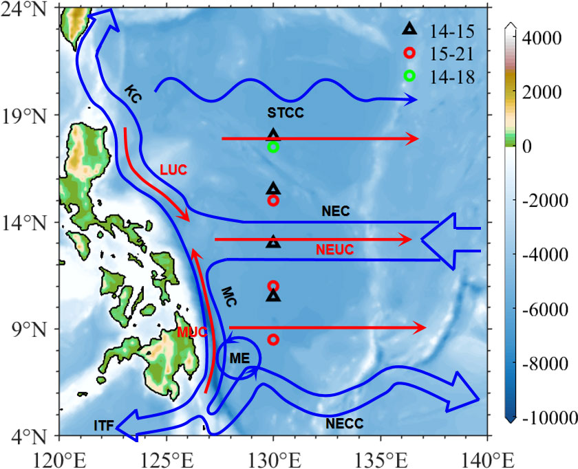
Figure 1 Location of the subsurface mooring array at 130°E. Black triangles denote the moorings deployed during September 2014 and September 2015 at 10.5°N, 13°N, 15.5°N and 18°N, red circles represent the moorings deployed during September 2015 and December 2021 at 8.5°N, 11°N, 12.5°N, and 15°N, and green circle represents the mooring deployed during September 2015 and January 2018 at 17.5°N. The mean ocean circulation system in this region is shown by red and blue arrows. NEC, NECC, STCC, KC, MC, NEUC, LUC, MUC, ME, and ITF stand for North Equatorial Current, North Equatorial Countercurrent, Subtropical Countercurrent, Kuroshio Current, Mindanao Current, North Equatorial Undercurrent, Luzon Undercurrent, Mindanao Undercurrent, Mindanao Eddy, and Indonesian Throughflow, respectively.

Each mooring was equipped with two RD Instruments (RDI) 75-kHz Acoustic Doppler Current Profilers (ADCPs) on the main float at the depth of 450 m, one of which looks upward and the other looks downward to collect the velocity data hourly. The standard bin size is 8 m, and the two ADCPs are able to capture the currents in the upper 900 m. In this work, the velocity raw data was first processed with standard quality control procedures, and the data with Percent Good 4 (PG4) value (a measure of the percentage of good data collected by the four beams of the ADCP) less than 85% was removed. Then, the hourly velocity was interpolated vertically onto 10 m intervals, and was daily averaged to remove tidal signals. The measurements above 40 m were dropped due to their large biases produced by the backscattering noise from the sea surface. It should be noted that there are one mooring lost and a couple of ADCPs failing to record the data due to instrument damages. Details of the moorings that have ADCP records are listed in Table 1. For convenience, all the records from nine moorings were processed onto five mooring sites at 8.5°N, 11°N, 12.5°N, 15°N, and 17.5°N. In detail, we made corrections to the mooring data at 10.5°N, 13°N, 15.5°N and 18°N before September 2015 by considering the meridional structure of the mean zonal flow at 130°E derived from high-resolution (0.25°×0.25°) T/S profiles of World Ocean Atlas 2018 (WOA18, Garcia et al., 2019). For example, the meridional difference of mean zonal flow between 10.5°N and 11°N was estimated first with WOA18. Then, the mooring data at 10.5°N before September 2015 was corrected with this meridional difference, and the obtained results was considered to be the velocity information at 11°N. Further, the data was merged with the ADCP measurements at 11°N after September 2015. Similar corrections were also made to the ADCP measurements at other latitudes. In addition, several discrete single-point current meters (CMs) distributed between 1000-4000 m on each mooring, including Nortek Aquadopp, ALEC and Aanderaa Seaguard current meters. The vertical interval between these current meters is about 500 m. Their observation period is the same as that of the ADCPs mentioned above, and the sampling period is 1 hour. These CM records will be used in the vertical mode projection in Section 3.4. The vertical mode projection needs the time series of velocity profile over the full depth. But the deep current meter records at 12.5°N for 2019 are abnormal due to instrumental malfunctions, and the current meter records at 17.5°N are only above 1400 m, which are insufficient for the projection. Considering better vertical coverage and continuity of the time series, the current meter records at 8.5°N, 11°N and 15°N were used in the vertical mode projection. Since this work mainly focuses on the interannual variations of the NEC/NEUC, the mooring data were therefore smoothed with a 1-year low-pass filter (moving average) to remove the intraseasonal and seasonal signals, and the values in the first 6 months and last 5 months were abandoned due to the bias near the endpoints of the time series caused by the filter. The filtered time series were used in the following analysis.

TABLE 1

Table 1 Mooring locations along 130°E and corresponding ADCP observation periods.

The gridded Sea Surface Height (SSH) and geostrophic currents from the AVISO (Archiving, Validation, and Interpretation of Satellite Oceanographic) products were also utilized in this study. This dataset merges measurements from different satellites such as Topex/Poseidon, European Remote Sensing Satellite-1 (ERS-1), ERS-2, Geosat Follow-On, Jason-1 and Jason-2. The daily data with the resolution of 0.25°×0.25° for the period of 2001-2021 was downloaded from the Copernicus Marine Environment Monitoring Service (CMEMS) website, and then averaged to obtain monthly time series. Details of the AVISO products are available in Boebel and Barron (2003) and Barron et al. (2009).

In addition, the monthly wind data from the fifth generation of European Centre for Medium-range Weather Forecasting (ECMWF) reanalysis (ERA5) with the resolution of 0.25°×0.25° during 1993-2021 was utilized in this study. It was provided by the Copernicus Climate Change Service (C3S), and the gridded monthly wind speed vector at 10-meter above the sea surface was used to derive the wind stress curl, which was then used to force the 1.5 layer reduced gravity model. The temperature anomalies in this study were derived from the gridded Argo observations since 2014, detailed descriptions can be referred to Roemmich and Gilson (2009).

Results

Mean structure of the NEC/NEUC

Figure 2 shows the time series of zonal velocity measured by mooring ADCPs along 130°E at different latitudes. By and large, the NEC exists stably between 8°N-18°N during the whole observation period from March 2015 to July 2021, while the NEUC beneath that appears intermittently at most of the latitudes. It is obvious that the intensity of NEC/NEUC is stronger at 8.5°N, 11°N, 12.5°N, compared with that at the other two latitudes, while the depth of the NEC deepens with increasing latitudes. Since the ADCP at 8.5°N well captures the structure and variability of the NEC and NEUC, we described the ADCP measurements at this site as an example (Figure 2E). The energetic westward-flowing NEC at this latitude is located in the upper 200 m, with the strongest current appearing in December 2017 and March 2021, with the velocity reaching -0.25 m/s at the depth of 70 m and -0.22 m/s at the depth of 90 m, respectively. Below 200 m, there appears to be an intermittent eastward-flowing NEUC, which seems to be associated with interannual events. It is strong during the period of March 2016-April 2017 and June 2019-June 2020 with the maximum velocity of 0.14 m/s at 430 m and 0.10 m/s at 400 m, when the overlying NEC is weak and shallow. During April 2017-November 2018 and October 2020-July 2021, the NEUC becomes weak, while the NEC strengthens and deepens. Notably, an obvious eastward flow appears in the upper 200 m during March-August 2015 at 17.5°N (Figure 2A), which is probably related to the Subtropical Countercurrent (STCC). STCC is a surface-trapped eastward flow in the upper 200 m with multiple branches between 17°N and 25°N (e.g., Yoshida and Kidokoro, 1967; Kobashi et al., 2006). Based on ADCP records along 135°E and satellite altimetry, a recent study demonstrated that the southern STCC is profoundly intensified by the mesoscale/sub-mesoscale eddy activities in El Niño (Azminuddin et al., 2019). Therefore, the northern part of the NEC could also be affected by meridional fluctuations of the STCC.

FIGURE 2

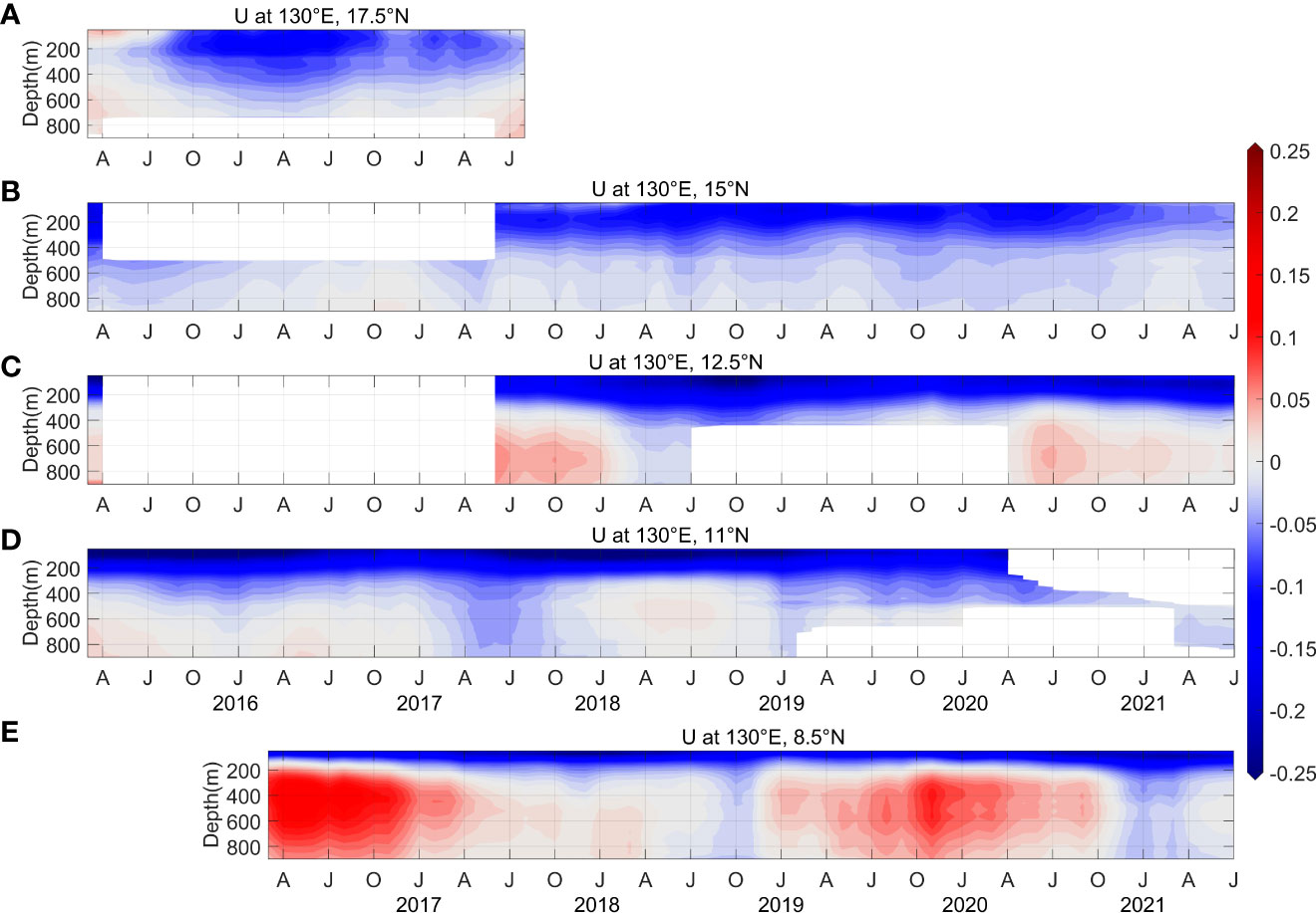
Figure 2 Time series of zonal velocity (m/s) measured by the mooring ADCPs at (A) 17.5°N, (B) 15°N, (C) 12.5°N, (D) 11°N and (E) 8.5°N along 130°E. All the time series have been smoothed with a 1-year low-pass filter.

In order to examine the mean velocity structure of the NEC/NEUC along the 130°E section, the temporally mean zonal current derived from moorings at different latitudes is shown in Figure 3. It is obvious that the main body of the NEC is concentrated above the isopycnal of 26.8 σ_θ, and therefore 26.8 σ_θ is considered as the bottom boundary of the NEC in this study. The velocity core of the NEC is located in the upper 100 m south of 12.5°N with a maximum of -0.24 m/s, and it deepens to 200 m with increasing latitudes. Below 26.8 σ_θ, two pronounced NEUC jets appear at ~8.5°N and ~12.5°N with a zonal velocity of 0.042 m/s and 0.024 m/s, respectively. An eastward flow with a velocity of 0.017 m/s is also observed below the depth of 600 m at ~17.5°N. Qiu et al. (2013b) and Wang et al. (2015) suggested that the northern branch of the NEUC is located around 18°N based on Argo and CTD data. Therefore, the eastward flow below 600 m at 17.5°N is believed to be associated with the northern NEUC jet, and the ADCP captures the upper part of the jet. Furthermore, the NEUC at 8.5°N seems stronger than that at the other two latitudes. The depth of NEUC jet is below 200 m at 8.5°N, which deepens gradually and reaches 600 m at 17.5°N. These results are generally consistent with the mean velocity structure derived from Argo floats and CTD measurements by previous studies in terms of the position and strength of the currents (e.g., Qiu et al., 2013b; Wang et al., 2015). The mean volume transports of the NEC and NEUC estimated from the ADCP measurements are -30.4 Sv and 5.1 Sv, respectively. Here, the NEC transport was defined as the integral of negative velocities from surface to 26.8 σ_θ between 8.5°-17.5°N, and the NEUC transport was calculated by integrating positive velocities from 26.8 σ_θ to 900 m between 8.5°-17.5°N. Based on multiple glider transects along 134.3°E between 8.5°-16.5°N, the mean NEC transport from the surface to 27.3 σ_θ is around -37.6 Sv with a standard deviation of 15.6 Sv (Schönau and Rudnick, 2015), and the ADCP-derived NEC transport generally agrees with the glider observations.

FIGURE 3

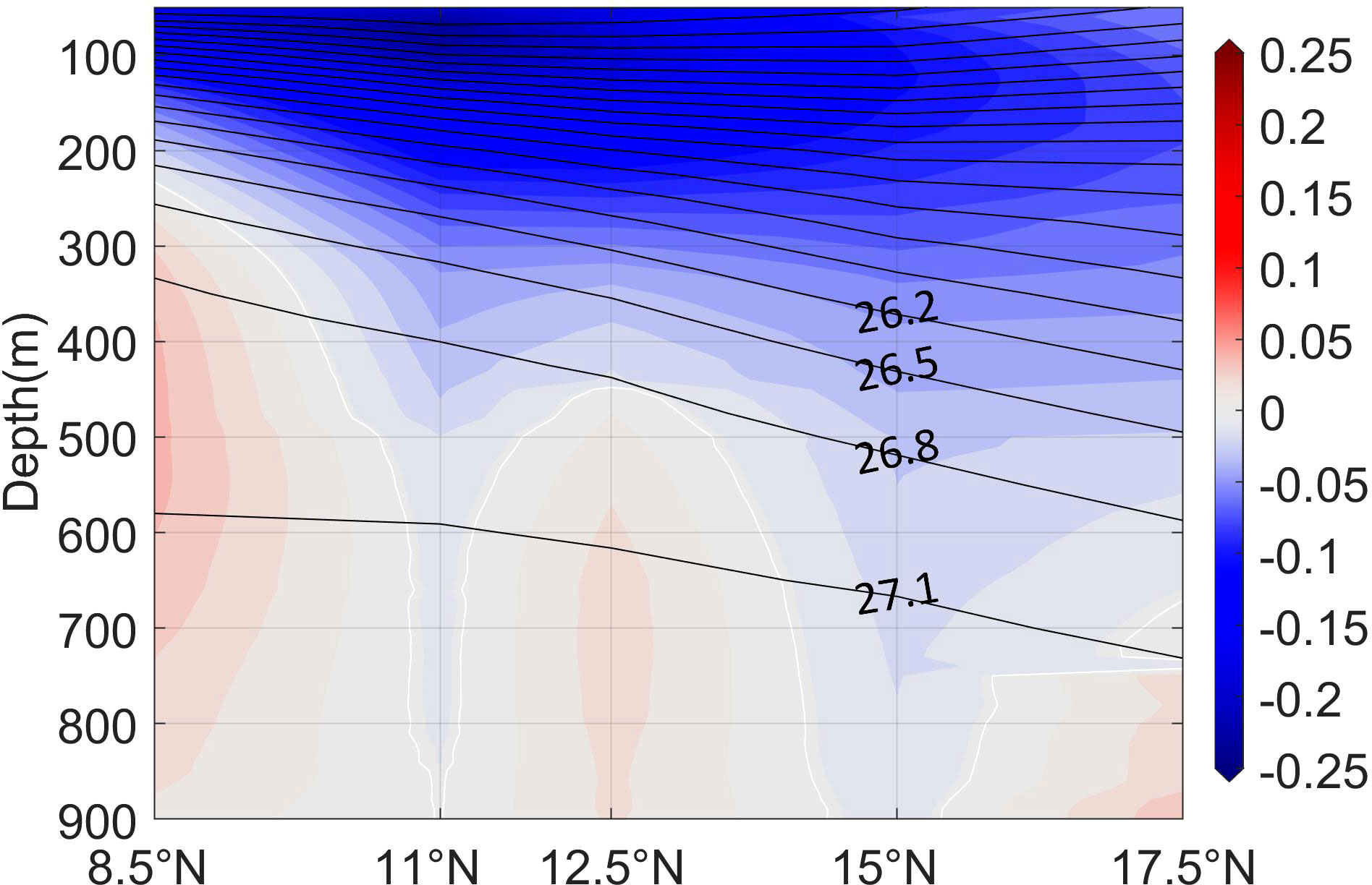
Figure 3 Mean zonal velocity (color, m/s) along 130°E section derived from all the mooring ADCP measurements during 2014-2021. Black curves denote potential density surfaces derived from WOA18.

Interannual variation of NEC/NEUC

Seven years of ADCP measurements enable us to explore the interannual variability of the NEC/NEUC. Figure 4 shows the time series of zonal velocity anomalies derived from mooring ADCP records at different latitudes. Significant variations of the currents could be noticed on interannual time scale. Interestingly, the zonal velocity in the upper 900 m at 8.5°N and 17.5°N exhibits prominent vertically synchronous fluctuations. For example, positive velocity anomalies appear in both the surface and subsurface layers from March 2016 to March 2017 and from April 2019 to July 2020 at 8.5°N, which turns into negative anomalies simultaneously from April 2017 to October 2018 and from October 2020 to July 2021 (Figure 4E). The vertically synchronous fluctuations also exist at 17.5°N (Figure 4A). Such vertically synchronous fluctuations in the upper 900 m imply that the eastward NEUC is strong when the overlying westward NEC is weak. This phenomenon coincides well with recent repeated glider observations by Schönau and Rudnick (2015). They suggested that persistent eastward undercurrents affected the transport variability of the NEC, with the NEC being weaker when there was a stronger NEUC. Therefore, their vertically synchronous fluctuations might be controlled by the same mechanism. Notably, the currents exhibit subsurface-intensified interannual features at 8.5°N with the strongest signal appearing between 300-500 m, and the signal is surface-intensified at 17.5°N, indicating different oceanic processes occur between these two latitudes. In addition, the interannual variation of the currents in the upper 900 m between 11°N and 15°N is not always vertically synchronous over the observation period (Figures 4B–D), implying the multimodal vertical structure of the interannual signal at these latitudes, which will be investigated in section 3.4.

FIGURE 4

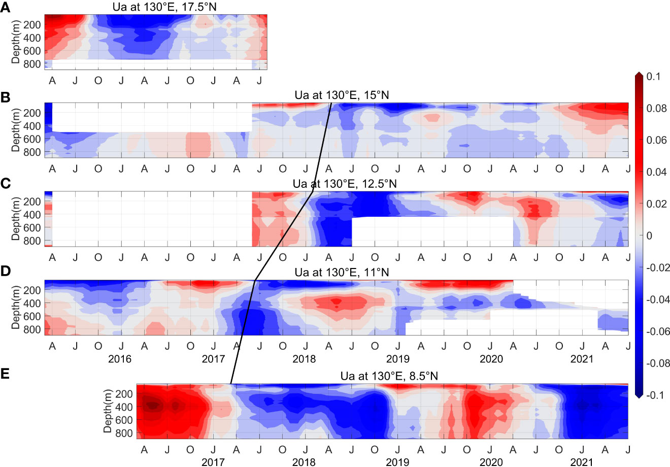
Figure 4 Time series of zonal velocity anomalies (m/s) derived from mooring ADCP measurements at (A) 17.5°N, (B) 15°N, (C) 12.5°N, (D) 11°N, and (E) 8.5°N along 130°E. All the time series have been smoothed with a 1-year low-pass filter.

In addition, there seems to be a meridional phase lag between the zonal velocity anomalies at different latitudes on interannual time scale, with the signal at higher latitudes lagging that at lower latitudes (Figure 4). For example, positive velocity anomalies shift to negative velocity anomalies that appears in March 2017 at 8.5°N, in June 2017 at 11°N, in February 2018 at 12.5°N, and in April 2018 at 15°N (Figures 4B–E). The signal at 15°N lags that at 8.5°N by about one year. To further examine the reliability of this meridional phase lag phenomenon, the lagging time was quantified by performing a lead-lag analysis to the time series of velocities averaged in the upper 200 m between every two adjacent sites from 8.5°N to 15°N. The results suggest that the interannual signal at 11°N lags that at 8.5°N by 3 months with a correlation of 0.81, the signal at 12.5°N lags that at 11°N by 8 months with a correlation of 0.77, and the signal at 15°N lags that at 12.5°N by 4 months with a correlation of 0.52. All of the correlations are significant at the 95% confidence level. Therefore, the phase lag of the zonal velocity at different latitudes is reliable. Recent study based on the same ADCP datasets along 130°E and satellite altimetry demonstrated a similar phase lag feature on seasonal time scale except for a slight phase advance from 8°N to 13°N (Wang et al., 2019). The propagation speed change of Rossby wave with latitudes plays a key role in explaining the phase lag feature, and the slight phase advance was attributed to the Asian monsoon (Wang et al., 2019). The difference of lead-lag relations on different time scales implies that the mechanism of the phase lag on interannual time scale might be different, which will be explored in the following analysis.

Considering the significant fluctuations of the velocity in the upper ocean observed by the ADCP measurements, the interannual variation of the currents should be captured well by the satellite altimetry. We firstly compared the altimeter-derived zonal currents with the mooring ADCP measurements, and the two time series agreed well with each other (Figure 5). The correlation between them is 0.74, 0.71, 0.96, 0.77, and 0.97 at 8.5°N, 11°N, 12.5°N, 15°N and 17.5°N, respectively, all of which are above the 95% confidence level. The high correlation indicates that the interannual variability of the currents detected by mooring ADCPs is well reflected by the satellite altimetry. Moreover, the meridional phase lag characteristics of the zonal velocity time series with latitudes are also well captured by the satellite altimetry. The large scale coverage of satellite observations enables us to further investigate the interannual variation of the currents in this region.

FIGURE 5

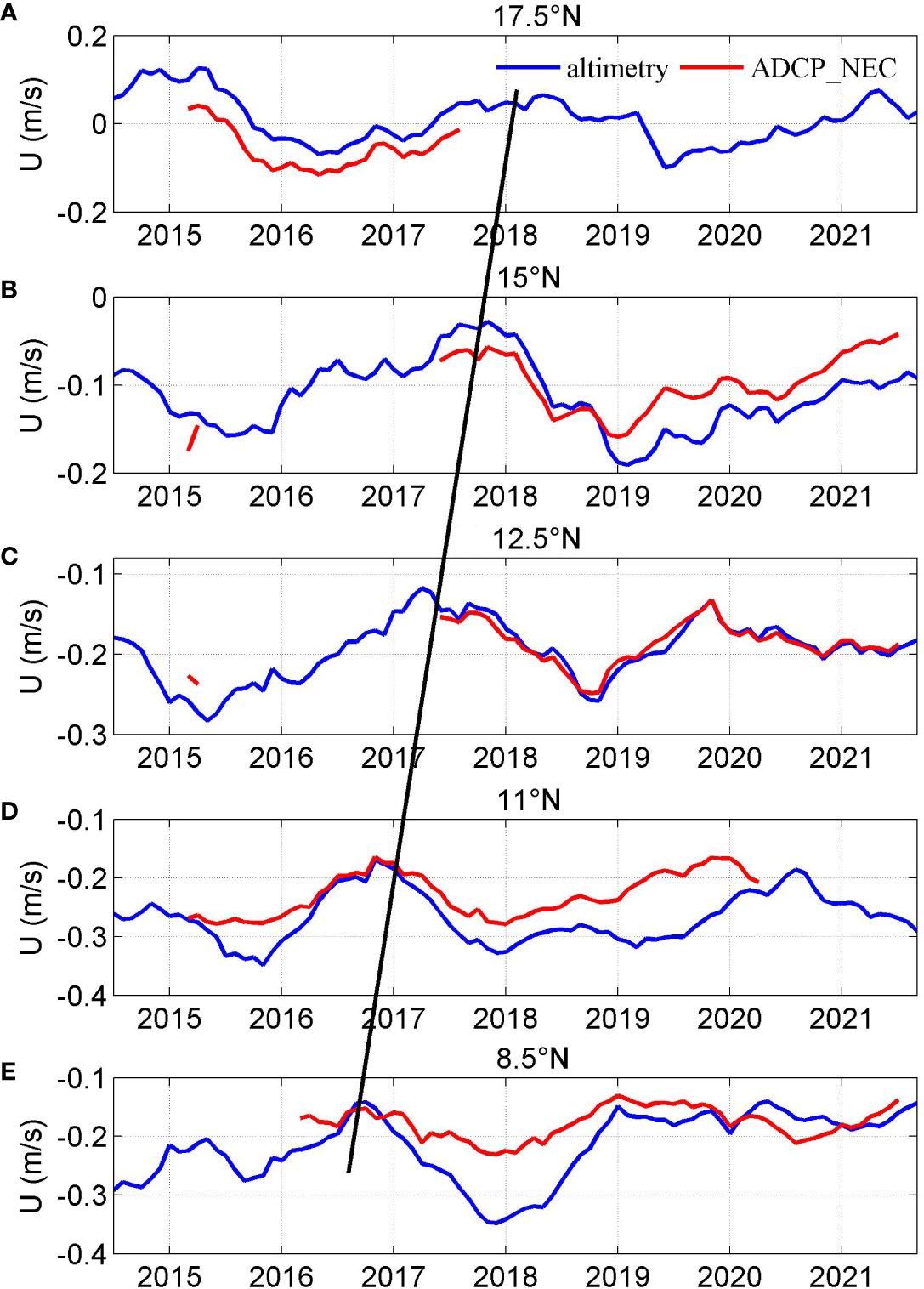
Figure 5 Vertically averaged zonal velocity (m/s) between 50-100 m derived from mooring ADCP measurements (red) at (A) 17.5°N, (B) 15°N, (C) 12.5°N, (D) 11°N and (E) 8.5°N during 2014-2021, compared with the zonal geostrophic velocity (m/s) at the same locations derived from satellite altimetry (blue). All the time series have been smoothed with a 1-year low-pass filter.

Figures 6A, C show the Sea Surface Height Anomalies (SSHA) and corresponding zonal geostrophic velocity anomalies at 130°E between 8°-18°N derived from satellite altimetry (2014-2018). The time series were moving-averaged in every 3° latitude band to avoid the influence of mesoscale features. Obviously, there are phase-lagged signals in the velocity with increasing latitudes. A positive velocity signal appears in July 2016 at 8.5°N, and then appears in November 2017 at 15°N, which is consistent with the results in Figures 4–5. The associated SSHA signals also exhibit pronounced phase-lagged features with latitudes (Figure 6A). The meridional gradient of this phase-lagged SSHA explains the delayed signal in the velocity anomalies shown in Figure 6C, and the reason for the phase-lagged SSHA will be given in the next section.

FIGURE 6

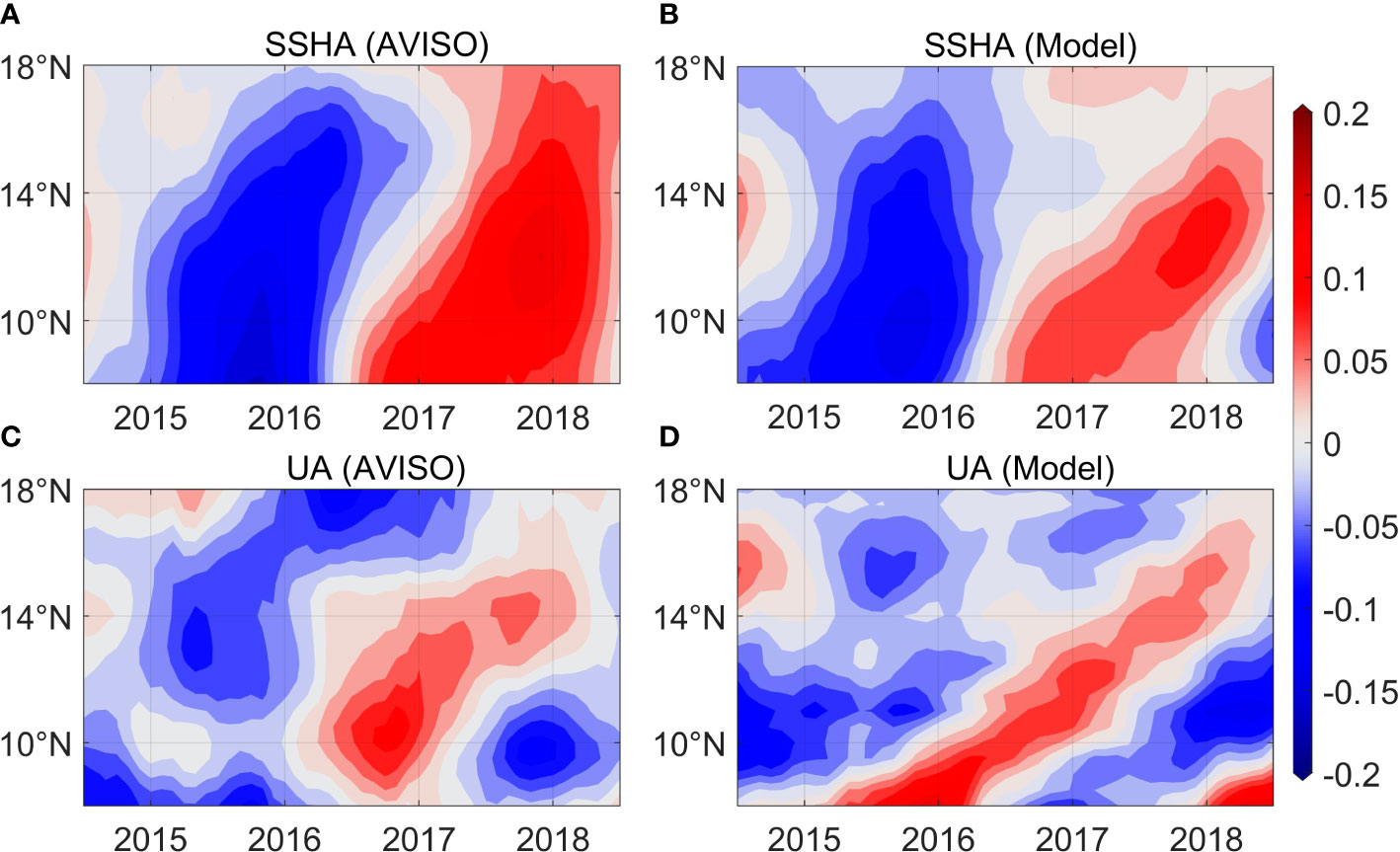
Figure 6 Time-latitude diagrams of the SSHA (a, m) and zonal geostrophic velocity anomalies (c, m/s) at 130°E derived from AVISO products. (B) and (D) are same as (A) and (C), but from reduced gravity model simulations.

Mechanism of the meridional phase lag

Interannual variations of SSHA in the western Pacific have been investigated in many previous studies, which were attributed to the basin-scale wind stress curl forcing. SSHA signals are induced by anomalous wind stress curl forcing in the central Pacific through Ekman convergence or divergence process, and then propagate westward in the form of baroclinic Rossby wave and modulate the SSH in the western Pacific (e.g., Qiu and Joyce, 1992; Qiu and Lukas, 1996; Qu et al., 1998; Kim et al., 2004; Kashino et al., 2009). Considering the different phase speed of the baroclinic Rossby wave at different latitudes, similar Rossby wave signals at low latitudes arrive to the western Pacific earlier than that at high latitudes due to its faster propagation speed, which may explain the meridional phase lag of velocity variations at different latitudes. We plotted the time-longitude diagrams of SSHA at 8.5°N, 12°N and 15°N during 2014-2018 in Figure 7. Obvious westward propagating signals could be noticed at all the latitudes, and positive/negative SSHA signals are induced by anomalous wind stress curl in the central Pacific, which arrive to the western Pacific earlier at 8.5°N than that at 15°N, reflecting the faster phase speed of the baroclinic Rossby wave at lower latitudes.

FIGURE 7

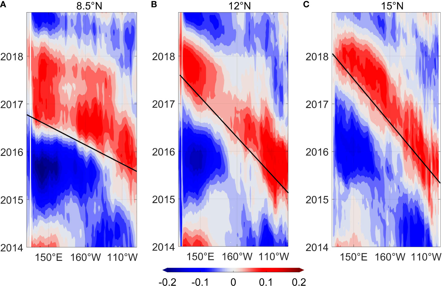
Figure 7 Hovmöller diagrams of the SSHA (m) along (A) 8.5°N, (B) 12°N, and (C) 15°N from AVISO products during January 2014 and December 2018.

To further investigate the effects of different baroclinic Rossby wave propagation speeds at different latitudes on the meridional phase lag of SSHA, we considered a linear wind-driven first-mode baroclinic Rossby wave model with zero background flow (e.g., Meyer, 1979; Kessler, 1990; Hsin and Qiu, 2012). Qiu and Chen (2006) pointed out that the east boundary forcing was important for capturing the observed SSHA at low latitudes, especially during strong ENSO events. Therefore, besides the wind stress curl forcing, the eastern boundary forcing is also included in the model, and the SSHA is estimated as follows,

$$h{\text{'}}_m(x,y,t)=\frac{g\text{'}}{g{\rho }_0}{\displaystyle {\int }_{x_e}^x\frac{1}{C_R(x\text{'},y)}\nabla \times \frac{\overrightarrow{\tau }(x\text{'},y,t+\frac{(x-x\text{'})}{C_R(x\text{'},y)})}{f(y)}·e^{\frac{ϵ(x-x\text{'})}{C_R(x\text{'},y)}}dx\text{'}}+h{\text{'}}_m(x_{\text{e}},y,t+\frac{x-x_{\text{e}}}{C_R})\exp [\frac{{\text{ε}}_{\text{B}}}{C_R}(x-x_{\text{e}})]$$

, $h{\text{'}}_m(x,y,t)$) denotes the modeled SSHA, and $h{\text{'}}_m(x_{\text{e}},y,t)$ is for the observed monthly SSHA near the Pacific eastern boundary (Fu and Qiu, 2002). C_R is the phase speed of the first-mode baroclinic Rossby wave. $\overrightarrow{\tau }$ is the wind stress vector, which is derived from the wind data of ERA5. g and ρ₀ are the gravity constant and background potential density of 9.807 m/s² and 1025 kg/m³, respectively. g’ is the reduced gravity. ε is the Newtonian dissipation rate, and ε_B is the Newtonian dissipation rate associated with the boundary-forced signals. The selection principle of g’, ε and ε_B is to make sure the difference between model results and observations reaches the minimum. For the baroclinic Rossby wave speed C_R, the value estimated by Chelton et al. (1998) based on the global climatological atlas of first-mode baroclinic gravity wave was used, which was further modified with a latitude-dependent amplification factor $\alpha (\text{y)}=1+0.06\times (\text{y-}10°N)$, to make the estimated C_R closer to the satellite altimeter observations, as suggested by Qiu and Chen (2006).

The simulated-SSHA and corresponding geostrophic velocity are shown in Figures 6B, D, respectively. The simulated-SSHA also displays meridional phase lag signals between 8°-16°N (Figure 6B), which is generally consistent with the satellite altimetry results (Figure 6A). The slight discrepancy between the observed and simulated SSHA could be related to energetic mesoscale eddy activities in this region. Mooring observations at 130°E revealed significant intraseasonal variations and active eddy activities (Zhang et al., 2017a), and mesoscale eddies could modulate the SSH variations through eddy momentum flux forcing (Qiu et al., 2015a). However, the reduced gravity model used here only captures the wind-driven SSH signals and misses the eddy-driven parts, which probably explains the difference between the observed and simulated SSHA (Figures 6A, B). In terms of the simulated velocity anomalies, the meridional phase lag signal with latitudes is obvious (Figure 6D). This result coincides well with the lag time demonstrated by the ADCP observations and satellite altimetry products. Above consistency between the model results and observations confirms that the interannual variation of the currents and SSHA at 130°E in the western Pacific is primarily determined by the wind stress curl variation through westward propagation of Rossby wave, and the different phase speed of the baroclinic Rossby wave at different latitudes accounts for the meridional phase lag of SSHA and associated geostrophic currents observed at the fixed longitude of 130°E.

To distinguish the contribution of wind forcing in different longitude bands, several wind-shield sensitivity experiments were performed with the 1.5 layer reduce-gravity model, which was forced by wind stress curl in the western (120°E-150°E), central (150°E-160°W) and eastern (160°W-110°W) Pacific, independently. The effect of eastern boundary forcing was also investigated with the model. The wind-shield sensitivity experiments at 8.5°N were displayed as an example (Figures 8A–F), and the time series of SSHA at 130°E derived from these experiments were shown in Figure 8G. The relative contribution of each regional wind forcing was further estimated as the standard deviation of the simulated time series divided by the sum of all the standard deviations. The results show that the wind forcing in the western, central, eastern Pacific, and the eastern boundary forcing explains 22.2%, 58.7%, 16.6% and 2.6% of the total interannual variations of the currents at 130°E, respectively. In addition, the wind-shield sensitivity experiments were also performed at 12.5°N and 15°N. The wind forcing in the western, central, eastern Pacific, and the eastern boundary forcing explains 20.4%, 56.8%, 17% and 5.8% of the total variance at 12.5°N, and explains 22.1%, 49.7%, 22.3% and 7.8% of the total variance at 15°N, respectively. Generally speaking, the wind forcing in the central Pacific plays a dominant role in the NEC variation at 130°E, and the wind forcing in the western and eastern Pacific also show substantial contributions, while the effect of eastern boundary forcing is limited.

FIGURE 8

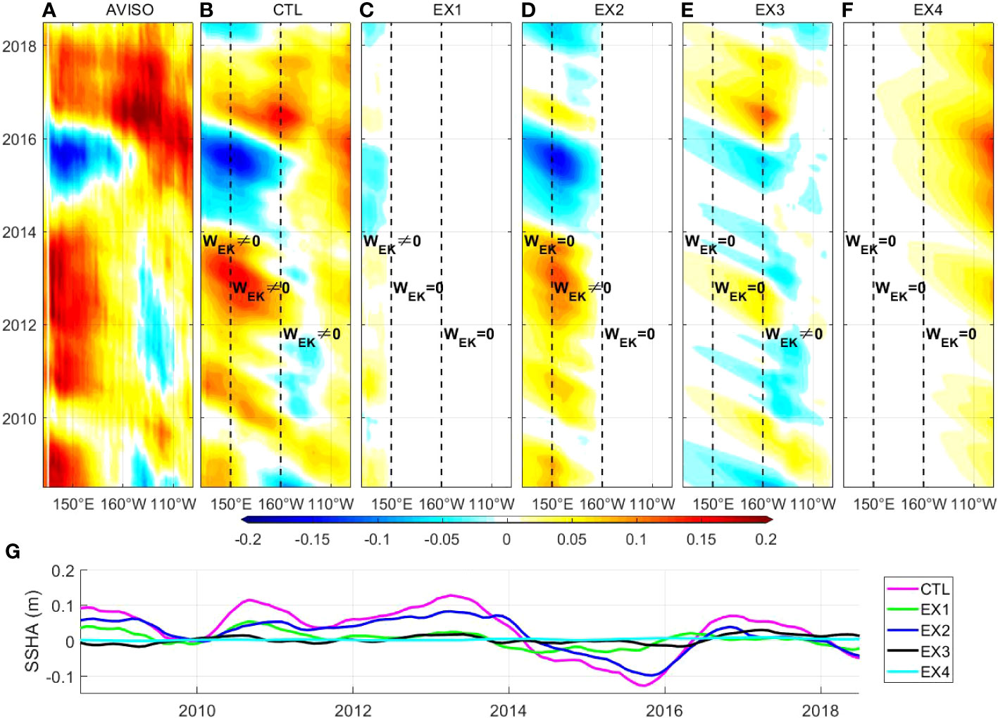
Figure 8 Hovmöller diagrams of SSHA (m) at 8.5°N derived from (A) altimeter observation and (B–F) model experiments with period longer than a year. (B) is forced by the wind stress curl from 130°E to 90°W and eastern boundary forcing. (C–E) are only forced by the wind stress curl between 130°-150°E, 150°E-160°W, and 160°-90°W, respectively. (F) is run with the eastern boundary forcing. (G) displays the time series of SSHA at 8.5°N, 130°E derived from above model experiments.

Mechanism of vertical variations

Mooring ADCP records reveal that the NEC/NEUC at 130°E exhibits pronounced vertical variations in the upper 900 m on interannual time scale. To investigate the vertical structure of this interannual variation, we calculated the empirical orthogonal function (EOF) mode of the velocity time series at different latitudes, and the pattern of the first EOF mode was shown in Figure 9. For zonal velocities at all the five mooring sites, the first EOF mode captures most part of the total velocity variance, which explains 93.3%, 45%, 86.5%, 73.6% and 96.4% of the total variance at 8.5°N, 11°N, 12.5°N, 15°N and 17.5°N, respectively. Obviously, the first EOF mode of the currents at 8.5°N seems intensified below the thermocline with the strongest signal appearing between 300-500 m. This subsurface-intensified signal also exists at 11°N, and gradually turns into a surface-intensified signal with increasing latitudes.

FIGURE 9

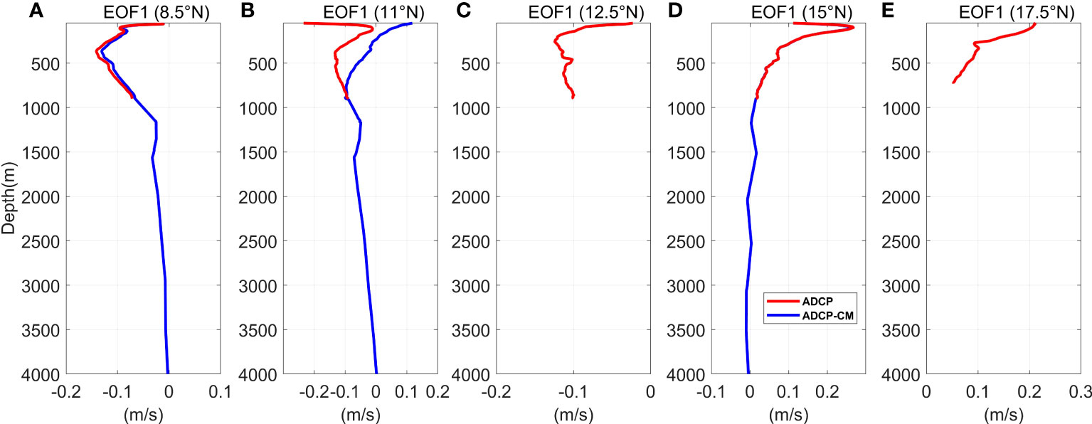
Figure 9 First EOF mode of the zonal velocity (m/s) time series at (A) 8.5°N, (B) 11°N, (C) 12.5°N, (D) 15°N, and (E) 17.5°N from mooring ADCP records in the upper 900 m (red) and ADCP-CM records in the upper 4000 m (blue).

Furthermore, we conducted EOF analysis to the time series of zonal velocity over the full depth by combining the ADCP measurements in the upper 900 m with the CM records between 1000-4000 m at 8.5°N, 11°N and 15°N (Figures 9A, B, D). The first EOF mode still plays a dominant role in the total velocity variations, which accounts for 86.7%, 48.1% and 65.3% of the total variance at 8.5°N, 11°N and 15°N, respectively. Both the surface-intensified signal at 15°N and subsurface-intensified signal at 8.5°N, 11°N are reflected in the first EOF mode over the full-depth, which coincides well with the EOF analysis in the upper 900 m mentioned above.

In fact, oceanic response to the wind forcing could be represented by the combination of signals with different vertical modes (e.g., McCreary, 1981; Kessler and McCreary, 1993). To explain the prominent difference of the first EOF mode among 8.5°-17.5°N, the vertical mode decomposition analysis was performed. Figure 10 shows the vertical structure of the barotropic mode and first three baroclinic modes at 8.5°N, 11°N, 12.5°N, 15°N and 17.5°N, which was estimated with the climatological mean density profile from the WOA18. Obviously, the first EOF mode at 15°N and 17.5°N show similar vertical structure to the first baroclinic mode, and the first EOF mode at 8.5°N, 11°N, and 12.5°N seem to be dominated by the combination of the first and second baroclinic mode (Figures 9 and 10).

FIGURE 10

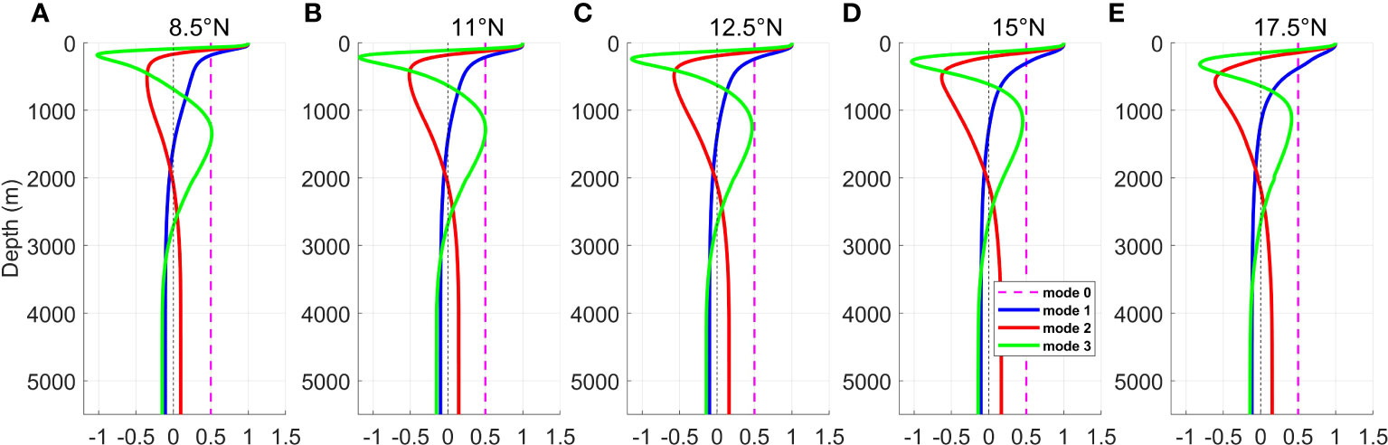
Figure 10 Vertical structure of the barotropic mode and first three baroclinic modes at (A) 8.5°N, (B) 11°N, (C) 12.5°N, (D) 15°N, and (E) 17.5°N along 130°E calculated with the climatological mean density profile from the WOA18.

We further projected the zonal velocity from ADCP and CM observations onto those vertical modes, and obtained the time series for each vertical mode. Considering the vertical mode projection needs the time series of velocity profile within the full-depth, the current meter records at 8.5°N, 11°N and 15°N were used due to their better vertical coverage and temporal continuity. The contribution of each mode was derived through calculating the standard deviation of each time series divided by the sum of all the standard deviations. The contribution of the first three baroclinic modes at each latitude was recorded in Table 2. Notably, the variance contribution of the first and second baroclinic mode reaches 45.38% and 13.81% at 15°N, demonstrating the dominance of the first baroclinic mode and accounting for the surface-intensified interannual variation of the NEC/NEUC velocity at this latitude (Figure 9D). While the contribution of the first baroclinic mode is comparable to that of the second baroclinic mode at the southern part, which reaches 32.99% and 29.9% at 8.5°N, and 32.76% and 23.59% at 11°N. It indicates that the second baroclinic mode substantially modulates the interannual variation of the currents, accounting for the subsurface-intensified characteristics of the interannual variation as revealed by the first EOF mode (Figures 9A, B).

TABLE 2

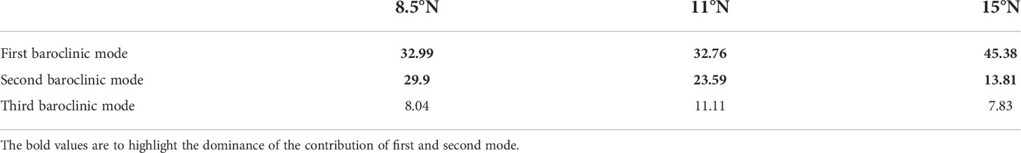
Table 2 Contribution (%) of the first three baroclinic modes at different latitudes.

In general, above analysis indicates that interannual variations of the NEC/NEUC velocity along 130°E between 8°-18°N are primarily dominated by surface-intensified signals with a vertical structure of the first baroclinic mode, while that in the southern part (8.5°N and 11°N) is also modulated by the second baroclinic mode, exhibiting subsurface-intensified features. We reconstructed the time series of velocity profile at 15°N with the first baroclinic mode and corresponding time series, and that at 8.5°N and 11°N with the first two baroclinic modes and their time series (Figure 11). The reconstructed time series at 8.5°N, 11°N and 15°N exhibit features consistent with the original time series from the moorings in Figure 4, further demonstrating the dominant role of these baroclinic modes in the interannual variation of the currents.

FIGURE 11

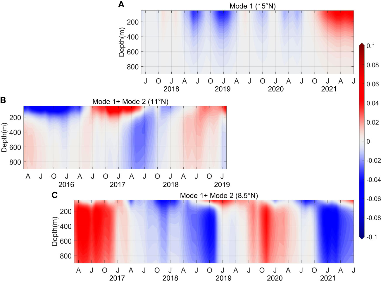
Figure 11 Reconstructed zonal velocity (m/s) time series in the upper 900 m during 2015-2021 with the first baroclinic mode at (A) 15°N, with (B) and (C) the first two baroclinic modes at 11°N, and 8.5°N.

Previous studies have investigated the excitation of different baroclinic vertical modes in response to wind stress forcing. Iskandar et al. (2006) adopted the wind stress coupling coefficient to examine the efficiency of the wind stress in exciting the vertical modes in the Indian Ocean, and concluded that the first mode was more favorably excited in thicker and milder thermocline regions, while the second mode was more efficiently excited in thinner and sharper thermocline regions. In this study, the basic density stratification along 130°E from 8°N to 18°N varies with latitudes. Hydrographic observations at 130°E indicated that the thermocline was thinner/sharper at 8.5°N, and thicker/milder at 15°N (Wang et al., 2015). Therefore, it is reasonable to hypothesize that the first baroclinic mode is excited more favorably at 15°N, while the second baroclinic mode is excited more favorably at 8.5°N, which to some extent explains the different vertical structure of the interannual variation observed by mooring ADCPs at different latitudes.

Relationship with ENSO

Interannual variations of the NEC are generally modulated by ENSO events (e.g., Qiu and Joyce, 1992; Qiu and Lukas, 1996), while the relationship between NEUC and ENSO events is not clear yet. Thus, this section attempts to discuss the relationship of NEUC with ENSO based on mooring observations. In fact, the mooring array used in this study well covers the NEC, but it seems insufficient to capture the NEUC branches due to their narrow width and active meridional shifts. Also, there are lots of gaps in the ADCP data due to instrument failure (Figure 2). These factors make it difficult to resolve the interannual variability of the multiple NEUC jets. Nevertheless, the ADCP data at 8.5°N is relatively continuous, and the jet appears stable, so this site is taken as an example to analyze the variability of the NEC/NEUC. Figure 12 displays the time series of NEC velocity vertically averaged between 50-150 m and NEUC velocity between 300-800 m derived from ADCP measurements at 8.5°N. The result indicates that the NEC variation is tightly correlated with Niño 3.4 index, which is weak during El Niño and strong during La Niña, considering that NEC is a westward flow. Previous studies demonstrated that the NEC migrated northward during El Niño and shifted to the south during La Niña (e.g., Qiu and Lukas, 1996; Kim et al., 2004; Qiu and Chen, 2010), which might be responsible for the interannual variation of NEC observed by ADCP at 8.5°N. Furthermore, the interannual variation of the NEUC branch at 8.5°N displays different features compared with that of the NEC, and it is intensified during the mature phase of El Niño and reaches the maximum velocity during the decay phase (Figure 12). When the NEUC velocity lags Niño3.4 index by 6 months, their correlation reaches maximum of 0.89, significantly above the 95% confidence level.

FIGURE 12

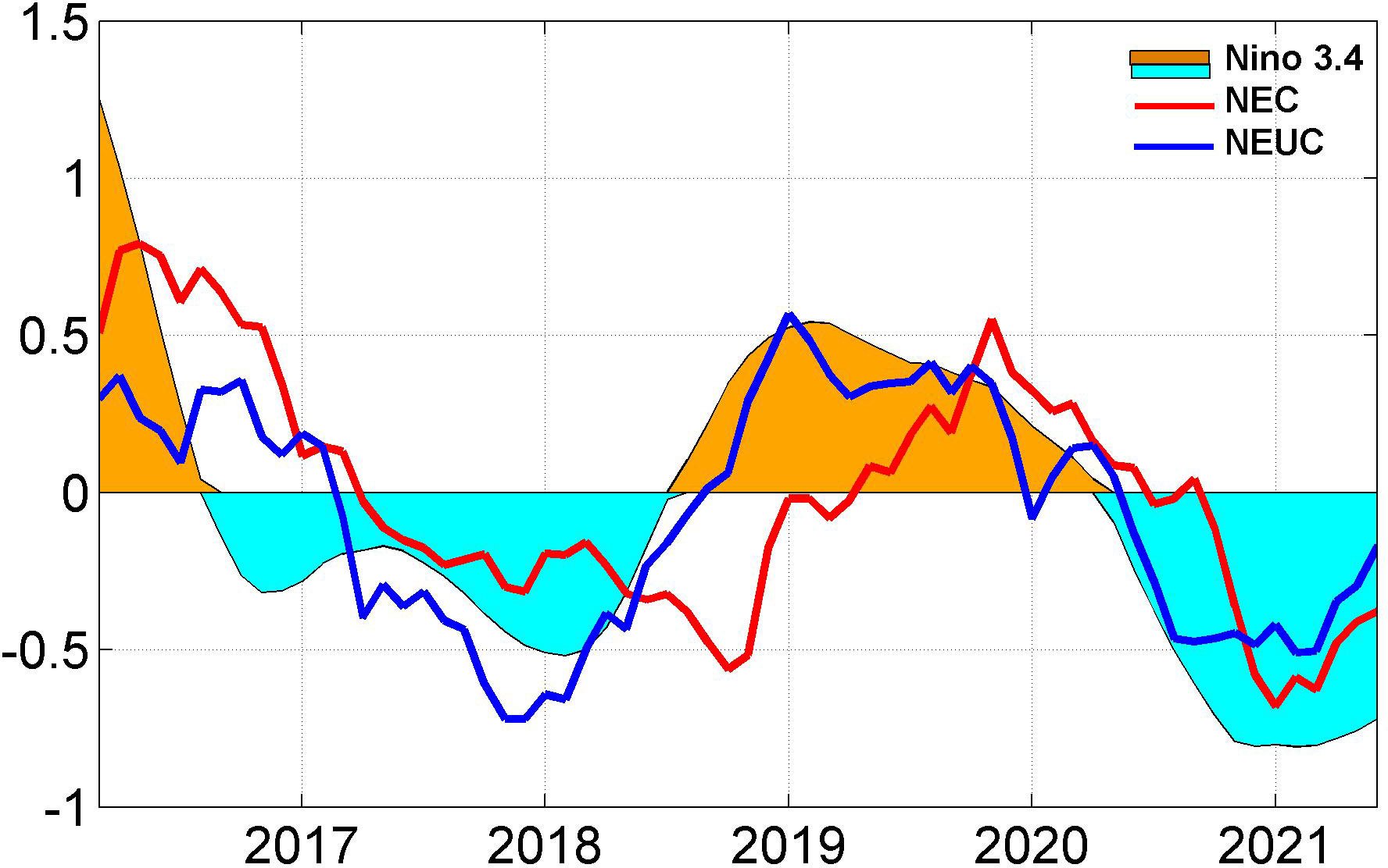
Figure 12 The normalized zonal velocity time series of NEC (blue) and NEUC (red) at 8.5°N derived from mooring measurements during 2016-2021. Shading denotes the Niño3.4 index. Here the normalized NEC velocity is defined as the mean zonal velocity averaged between 50-150 m, which is scaled by its standard deviation. The definition of normalized NEUC is same as the NEC but for the depth range of 300-800 m. All curves are smoothed with a 1-year low-pass filter.

To further demonstrate their interannual variations, the Hovmöller diagram of temperature anomalies in the NEC/NEUC layer (0-150/300-800 dbar) at 8.5°N was examined with Argo data (Figure 13). The temperature phases in the upper ocean are basically consistent with the interannual variation of the NEC (Figures 12 and 13A): cooling during the weakened phase of NEC (July 2014-July 2016 and July 2018-September 2019), and warming during the intensified phase of NEC (January 2017-April 2018 and January 2020-June 2021). For the NEUC layer, the temperature anomalies are relatively weaker but the pattern is similar to that in the NEC layer (Figure 13B). Westward propagating signals are noticeable in both the NEC and NEUC layer, indicating that the interannual variation of both the NEC and NEUC is influenced by the remote wind forcing through Rossby waves. Nevertheless, the positive temperature anomalies in the NEUC layer west of 150°E during August 2016-March 2018 and April 2020-April 2021 exhibit features generated locally (Figure 13B), implying that the interannual variability of the NEUC is probably also modulated by local factors besides the remote wind forcing.

FIGURE 13

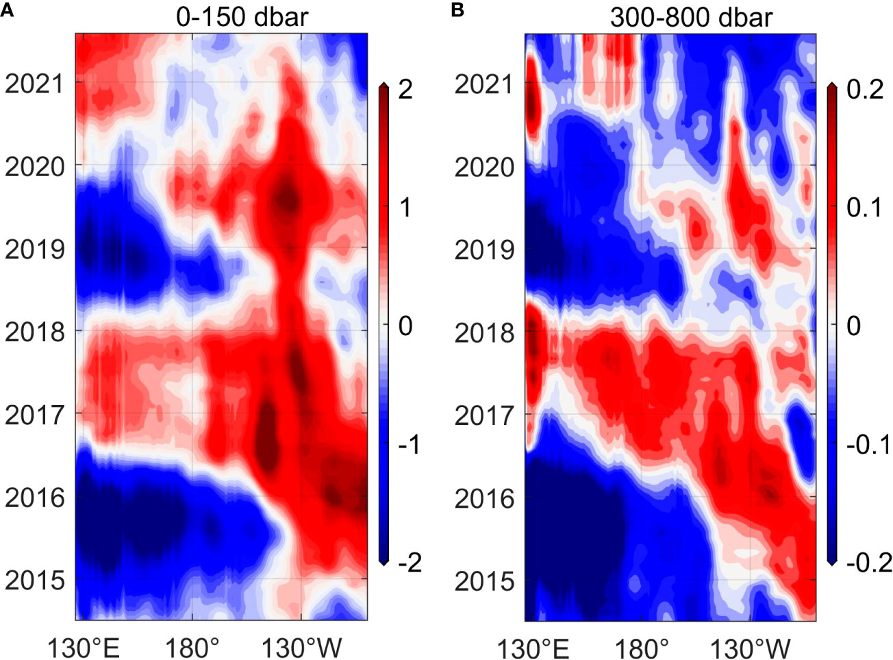
Figure 13 Hovmöller diagram of the temperature anomaly (°C) averaged between (A) 0-150 dbar and (B) 300-800 dbar at 8.5°N derived from Argo during 2014-2021. Note that the colorbar scale is different in (A) and (B).

Conclusion and discussion

Based on mooring observations along 130°E between 8°-18°N in the northwestern Pacific during 2014-2021, combining with AVISO products, the interannual variability of the NEC and NEUC was investigated. Seven years of mooring ADCP measurements in the upper 900 m indicate prominent interannual variations of the NEC and NEUC, with the interannual signal in the north lagging that in the south. Satellite altimetry also demonstrates consistent phase-lagged features with increasing latitudes. Utilizing a 1.5-layer reduced gravity model, interannual variations of the SSH and associated currents in this area were simulated. It is suggested that the meridional phase lag of velocity at different latitudes on the interannual time scale is related to the different propagating speed of baroclinic Rossby wave, which propagates faster at lower latitudes and slower at higher latitudes. Further model sensitivity experiments suggest that the wind forcing in the central Pacific plays a dominant role in the SSHA variation at 130°E, while the effects of wind forcing in the western and eastern Pacific are not ignorable.

EOF and vertical mode decomposition analysis indicate that interannual variation of the NEC/NEUC velocity structure at 130°E is mostly dominated by the first baroclinic mode with a surface-intensified structure. At 8.5°N and 11°N, the second baroclinic mode also modulates the interannual variation of the currents substantially, and the contribution is comparable to the first baroclinic mode, inducing the subsurface-intensified vertical structure of the interannual signal at these latitudes. The excitation of different baroclinic modes at different latitudes is probably related to the stratification change crossing the NEC/NEUC along 130°E.

The NEUC exhibits pronounced relationship with ENSO. Mooring measurements at 8.5°N indicates that the NEUC branch is intensified during the mature phase of El Niño, and reaches the maximum velocity during the decay phase. Its correlation with Niño 3.4 index reaches 0.89 when the NEUC lags by 6 months, and both the locally generated and westward propagating signals are important for the interannual modulation of NEUC at 130°E.

Previous studies associated the zonal velocity and temperature variations below the equatorial thermocline with vertically propagating equatorial Rossby waves (e.g., Kessler and McCreary, 1993; Marin et al., 2010; Ishizaki et al., 2014; Ma et al., 2020). Yang et al. (2020) utilized the linear continuously stratified model to investigate the oceanic response with different vertical modes and concluded that the seasonal variability of the subsurface currents in the northwestern tropical Pacific was more correlated to the vertical propagation of off-equatorial Rossby waves associated with low-order baroclinic modes in the stratified ocean than that of the equatorial Rossby waves. Statistical analysis (EOF and vertical mode decomposition) in this study indicates that interannual variations of the NEC/NEUC reflect the low-order mode baroclinic response of the ocean to wind forcing, but it is ambiguous what role the vertical propagation of off-equatorial Rossby waves plays in that process on interannual time scale. Therefore, a linear continuously stratified model will be employed in future works to examine the interannual variability of NEC/NEUC and its relationship with the vertical propagation of off-equatorial Rossby waves.

Data availability statement

The original contributions presented in the study are included in the article/Supplementary Material. Further inquiries can be directed to the corresponding author.

Author contributions

YH performed the data analysis and wrote the initial draft. LZ proposed the main ideas, took part in the data analysis, and dramatically modified the manuscript. FJW, FW, and DH all participated in the discussion and contributed to the improvement of the manuscript. All authors contributed to the article and approved the submitted version.

Funding

This study was funded by the Strategic Priority Research Program of the Chinese Academy of Sciences (No. XDB42010105), the National Key Research and Development Program of China (No. 2020YFA0608801), the National Natural Science Foundation of China (Grant No. 42122041), and the National Key Research and Development Program of China (No. 2017YFA0603202). The Youth Innovation Promotion Association (CAS) and the TS Scholar Program also supported this study. Mooring data were collected onboard of R/V KeXue implementing the open research cruises NORC2019-09 and NORC2021-09 supported by the NSFC Shiptime Sharing Projects (Grant No. 41849909 and 42049909) and QNLM shipboard observation cruise (Grant No. 2022QNLM010103).

Acknowledgments

We express our sincere gratitude to the crew of R/V Science, including all scientists and technicians on board for deployment and retrieval of subsurface moorings. This study was also benefited from the freely available datasets: satellite altimetry dataset (https://resources.marine.copernicus.eu/product-download/SEALEVEL_GLO_PHY_L4_MY_008_047), ERA5 wind dataset (https://cds.climate.copernicus.eu/cdsapp#!/dataset/reanalysis-era5-single-levels-monthly-means?tzab=form), Argo dataset (http://sio-argo.ucsd.edu/RG_Climatology.html), and WOA18 dataset (https://www.ncei.noaa.gov/access/world-ocean-atlas-2018/).

Conflict of interest

The authors declare that the research was conducted in the absence of any commercial or financial relationships that could be construed as a potential conflict of interest.

Publisher’s note

All claims expressed in this article are solely those of the authors and do not necessarily represent those of their affiliated organizations, or those of the publisher, the editors and the reviewers. Any product that may be evaluated in this article, or claim that may be made by its manufacturer, is not guaranteed or endorsed by the publisher.

Supplementary Material

The Supplementary Material for this article can be found online at: https://www.frontiersin.org/articles/10.3389/fmars.2022.979442/full#supplementary-material

References

Azminuddin F., Jeon D., Shin C. W. (2019). Intraseasonal-to-interannual variability of the upper-layer zonal currents in the tropical northwest pacific ocean. Ocean Sci. J. 54, 15–27. doi: 10.1007/s12601-019-0001-2

CrossRef Full Text | Google Scholar

Barron C. N., Kara A. B., Jacobs G. A. (2009). Objective estimates of westward rossby wave and eddy propagation from sea surface height analyses. J. Geophysical Res. 114 (C3), C03013. doi: 10.1029/2008JC005044

CrossRef Full Text | Google Scholar

Boebel O., Barron C. (2003). A comparison of in-situ float velocities with altimeter derived geostrophic velocities. Deep Sea Res. Part II: Topical Stud. Oceanography 50 (1), 119–139. doi: 10.1016/S0967-0645(02)00381-8

CrossRef Full Text | Google Scholar

Chelton D. B., deSzoeke R. A., Schlax M. G., El Naggar K., Siwertz N. (1998). Geographical variability of the first-baroclinic rossby radius of deformation. J. Phys. Oceanography 28, 433–460. doi: 10.1175/1520-0485(1998)028<0433:GVOTFB>2.0.CO;2

CrossRef Full Text | Google Scholar

Chen Z., Wu L. (2011). Dynamics of the seasonal variation of the north equatorial current bifurcation. J. Geophysical Res. 116, C02018. doi: 10.1029/2010JC006664

CrossRef Full Text | Google Scholar

Donguy J. R., Meyers G. (1996). Mean annual variation of transport of major current in the tropical pacific ocean. Deep-Sea Res. Part I 43, 1105–1122. doi: 10.1016/0967-0637(96)00047-7

CrossRef Full Text | Google Scholar

Fu L. L., Qiu B. (2002). Low-frequency variability of the north pacific ocean: The roles of boundary- and wind-driven baroclinic rossby waves. J. Geophysical Res. 107 (C12), 3220. doi: 10.1029/2001JC001131

CrossRef Full Text | Google Scholar

Garcia H. E., Boyer T. P., Baranova O. K., Locarnini R. A., Mishonov A. V., Grodsky A., et al. (2019). World ocean atlas 2018: Product documentation. Mishonov A, Technical Editor. Available at: https://data.nodc.noaa.gov/woa/WOA18/DOC/woa18documentation.pdf.

Google Scholar

Hsin Y. C., Qiu B. (2012). Seasonal fluctuations of the surface north equatorial countercurrent (NECC) across the pacific basin. J. Geophysical Research: Oceans 117 (C6), C06001. doi: 10.1029/2011JC007794

CrossRef Full Text | Google Scholar

Hu D., Wang F., Sprintall J., Wu L., Riser S., Cravatte S., et al. (2020). Review on observational studies of western tropical pacific ocean circulation and climate. J. Oceanology Limnology 38 (4), 906–929. doi: 10.1007/s00343-020-0240-1

CrossRef Full Text | Google Scholar

Hu D., Wang F., Wu L., Chen D., Liu Q., Tian J., et al. (2011). Northwestern pacific ocean circulation and climate experiment (NPOCE) (Beijing, China: China Ocean Press).

Google Scholar

Hu D., Wu L., Cai W., Gupta A. S., Ganachaud A., Qiu B., et al. (2015). Pacific western boundary currents and their roles in climate. Nature 522 (7556), 299–308. doi: 10.1038/nature14504

PubMed Abstract | CrossRef Full Text | Google Scholar

Ishizaki H., Nakano H., Nakano T., Shikama N. (2014). Evidence of equatorial rossby wave propagation obtained by deep mooring observations in the western pacific ocean. J. Oceanography 70, 463–488. doi: 10.1007/s10872-014-0247-3

CrossRef Full Text | Google Scholar

Ishizaki H., Nakano T., Nakano H., Yamanaka G. (2019). Interdecadal variability of the north equatorial undercurrent (NEUC) found in the long-term hydrographic observations along 137°E. J. Oceanography 75 (5), 395–414. doi: 10.1007/s10872-019-00509-6

CrossRef Full Text | Google Scholar

Iskandar I., Tozuka T., Sasaki H., Masumoto Y., Yamagata T. (2006). Intraseasonal variations of surface and subsurface currents off Java as simulated in a high-resolution ocean general circulation model. J. Geophysical Research: Oceans 111 (C12). doi: 10.1029/2006JC003486

CrossRef Full Text | Google Scholar

Kashino Y., Espana N., Syamsudin F., Richards K. J., Jensen T., Dutrieux P., et al. (2009). Observations of the north equatorial current, Mindanao current, and kuroshio current system during the 2006/07 El niño and 2007/08 la niña. J. Oceanography 65 (3), 325–333. doi: 10.1007/s10872-009-0030-z

CrossRef Full Text | Google Scholar

Kessler W. S. (1990). Observations of long rossby waves in the northern tropical pacific. J. Geophysical Res. 95 (C4), 5183–5127. doi: 10.1029/JC095iC04p05183

CrossRef Full Text | Google Scholar

Kessler W. S., McCreary J. P. (1993). The annual wind-driven rossby wave in the subthermocline equatorial pacific. J. Phys. Oceanography 23, 1192–1207. doi: 10.1175/1520-0485(1993)023,1192:TAWDRW.2.0.CO;2

CrossRef Full Text | Google Scholar

Kim Y. Y., Qu T., Jensen T., Miyama T., Mitsudera H., Kang H. W., et al. (2004). Seasonal and interannual variations of the north equatorial current bifurcation in a high-resolution OGCM. J. Geophysical Res. 109 (C3), C03040. doi: 10.1029/2003JC002013

CrossRef Full Text | Google Scholar

Kobashi F., Mitsudera H., Xie S. P. (2006). Three subtropical fronts in the north pacific: Observational evidence for mode waterinduced subsurface frontogenesis. J. Geophysical Res. 111, C09033. doi: 10.1029/2006JC003479

CrossRef Full Text | Google Scholar

Li Y., Liu H., Lin P. (2018). Interannual and decadal variability of the north equatorial undercurrents in an eddy-resolving ocean model. Sci. Rep. 8, 17112. doi: 10.1038/s41598-018-35469-2

PubMed Abstract | CrossRef Full Text | Google Scholar

Liu X., Zhou H. (2020). Seasonal variations of the north equatorial current across the pacific ocean. J. Geophysical Research: Oceans 125, e2019JC015895. doi: 10.1029/2019JC015895z

CrossRef Full Text | Google Scholar

Lukas R., Firing E., Hacker P., Richardson P., Collins C., Fine R., et al. (1991). Observations of the Mindanao current during the Western equatorial pacific ocean circulation study. J. Geophysical Res. 96, 7089–7104. doi: 10.1029/91JC00062

CrossRef Full Text | Google Scholar

Marin F., Kestenare E., Delcroix T., Durand F., Cravatte S., Eldin G. (2010). Annual reversal of the equatorial intermediatecurrent in the pacific: Observations andmodel diagnostics. J. Phys. Oceanography 40, 915–933. doi: 10.1175/2009JPO4318.1

CrossRef Full Text | Google Scholar

Ma Q., Wang J., Wang F., Zhang D., Zhang Z., Lyu Y. (2020). Interannual variability of lower equatorial intermediate current response to ENSO in the Western pacific. Geophysical Res. Lett. 47 (16), e2020GL089311. doi: 10.1029/2020GL089311

CrossRef Full Text | Google Scholar

McCreary J. P. (1981). A linear stratified ocean model of the equatorial undercurrent. Philos. Trans. R. Soc. London A298, 603–635. doi: 10.1098/rsta.1981.0002

CrossRef Full Text | Google Scholar

Meyers G. (1979). On the annual rossby wave in the tropical north pacific ocean. J. Phys. Oceanography 9 (4), 66–674. doi: 10.1175/1520-0485(1979)009<0663:otarwi>2.0.co;2

CrossRef Full Text | Google Scholar

Nitani H. (1972). “Beginning of the kuroshio,” in Kuroshio: Physical aspects of the Japan current. Eds. Stommel H., Yoshida &K. (Seattle, WA: University of Washington Press), pp.129–pp.163.

Google Scholar

Qiu B., Chen S. (2006). Decadal variability in the large-scale sea surface height field of the south pacific ocean: Observations and causes. J. Phys. Oceanography 36 (9), 1751–1762. doi: 10.1175/JPO2943.1

CrossRef Full Text | Google Scholar

Qiu B., Chen S. (2010). Interannual-to-Decadal variability in the bifurcation of the north equatorial current off the Philippines. J. Phys. Oceanography 40 (11), 2525–2538. doi: 10.1175/2010JPO4462.1

CrossRef Full Text | Google Scholar

Qiu B., Chen S., Sasaki H. (2013a). Generation of the north equatorial undercurrent jets by triad baroclinic rossby wave interactions. J. Phys. Oceanography 43 (12), 2682–2698. doi: 10.1175/JPO-D-13-099.1

CrossRef Full Text | Google Scholar

Qiu B., Chen S., Wu L., Kida S. (2015a). Wind-versus eddy-forced regional Sea level trends and variability in the north pacific ocean. J. Climate 28, 1561–1577. doi: 10.1175/JCLI-D-14-00479.1

CrossRef Full Text | Google Scholar

Qiu B., Joyce T. M. (1992). Interannual variability in the mid-and low-latitude western north pacific. J. Phys. Oceanography 22, 1062–1084. doi: 10.1175/1520-0485(1992)022<1062:IVITMA>2.0.CO;2

CrossRef Full Text | Google Scholar

Qiu B., Lukas R. (1996). Seasonal and interannual variability of the north equatorial current, the Mindanao current, and the kuroshio along the pacific western boundary. J. Geophysical Res: Oceans 101 (C5), 12315–12330. doi: 10.1029/95JC03204

CrossRef Full Text | Google Scholar

Qiu B., Rudnick D. L., Cerovecki I., Cornuelle B. D., Chen S., Mcclean J. L., et al. (2015b). The pacific north equatorial current: New insights from the origins of the kuroshio and Mindanao currents (OKMC) project. Oceanography 28 (4), 24–33. doi: 10.5670/oceanog.2015.78

CrossRef Full Text | Google Scholar

Qiu B., Rudnick D. L., Chen S., Kashio Y. (2013b). Quasi−stationary north equatorial undercurrent jets across the tropical north pacific ocean. Geophysical Res. Lett. 40 (10), 2183–2187. doi: 10.1002/grl.50394

CrossRef Full Text | Google Scholar

Qu T., Lukas R. (2003). The bifurcation of the north equatorial current in the pacific. J. Phys. Oceanography 33 (1), 5–18. doi: 10.1175/1520-0485(2003)033<0005:TBOTNE>2.0.CO;2

CrossRef Full Text | Google Scholar

Qu T., Mitsudera H., Yamagata T. (1998). On the western boundary currents in the Philippine Sea. J. Geophysical Res. 103, 7537–7548. doi: 10.1029/98JC00263

CrossRef Full Text | Google Scholar

Roemmich D., Gilson J. (2009). The 2004-2008 mean and annual cycle of temperature, salinity, and steric height in the global ocean from the argo program. Prog. Oceanography 82, 81–100. doi: 10.1016/j.pocean.2009.03.004

CrossRef Full Text | Google Scholar

Schonau M. C., Rudnick D. L. (2015). Glider observations of the north equatorial current in the western tropical pacific. J. Geophysical Research: Oceans 120 (5), 3586–3605. doi: 10.1002/2014JC010595

CrossRef Full Text | Google Scholar

Ueki I., Kashino Y., Kuroda Y. (2003). Observation of current variations off the New Guinea coast including the 1997-1998 El niño period and their relationship with sverdrup transport. J. Geophysical Res. 108, 3243. doi: 10.1029/2002JC001611

CrossRef Full Text | Google Scholar

Wang F., Hu D., Bai H. (1998). Western Boundary undercurrents east of the Philippines. Proc. 4th Pacific Ocean Remote Sens. Conf. (PORSEC) 98, 551–556.

Google Scholar

Wang F., Wang Q., Zhang L., Hu D., Hu S., Feng J. (2019). Spatial distribution of the seasonal variability of the north equatorial current. Deep Sea Res. Part I: Oceanographic Res. Papers 144, 63–74. doi: 10.1016/j.dsr.2019.01.001

CrossRef Full Text | Google Scholar

Wang F., Zang N., Li Y., Hu D. (2015). On the subsurface countercurrents in the Philippine Sea. J. Geophysical Research: Oceans 120, 131–144. doi: 10.1002/2013JC009690

CrossRef Full Text | Google Scholar

Wang Z., Zhang L., Hui Y., Wang F., Hu D. (2022). Two Flavors of Intraseasonal Variability and Their Dynamics in the North Equatorial Current/Undercurrent Region.Front. Mar. Sci 9, 845575. doi: 10.3389/fmars.2022.845575

CrossRef Full Text | Google Scholar

Yang Y., Li X., Wang J., Yuan D. (2020). Seasonal variability and dynamics of the pacific north equatorial subsurface current. J. Phys. Oceanography 50, 2457–2474. doi: 10.1175/JPO-D-19-0261.1

CrossRef Full Text | Google Scholar

Yoshida K., Kidokoro T. (1967). A subtropical counter-curreut in the north pacific–an eastward flow near the subtropical convergence. J. Oceanography Soc. Japan 23 (2), 88–91. doi: 10.5928/kaiyou1942.23.88

CrossRef Full Text | Google Scholar

Zhai F., Hu D. (2012). Interannual variability of transport and bifurcation of the north equatorial current in the tropical north pacific ocean. Chin. J. Oceanology Limnology 30 (1), 177–185. doi: 10.1007/s00343-012-1194-8

CrossRef Full Text | Google Scholar

Zhai F., Hu D. (2013). Revisit the interannual variability of the north equatorial current transport with ECMWF ORA-S3. J. Geophysical Research: Oceans 118 (3), 1349–1366. doi: 10.1002/jgrc.20093

CrossRef Full Text | Google Scholar

Zhang L., Wang F., Wang Q., Hu S., Wang F., Hu D. (2017a). Structure and variability of the north equatorial Current/Undercurrent from mooring measurements at 130°E in the Western pacific. Sci. Rep. 7, 46310. doi: 10.1038/srep46310

PubMed Abstract | CrossRef Full Text | Google Scholar

Zhang Z., Xue H., Chai F., Chao Y. (2017b). Variability of the pacific north equatorial current from 1993 to 2012 based on a 1/8° pacific model simulation. J. Geophysical Res: Oceans 122 (3), 2382–2400. doi: 10.1002/2016JC012143

CrossRef Full Text | Google Scholar