Assessing the ability of deep learning techniques to perform real-time identification of shark species in live streaming video from drones

1 Introduction

The threat of shark bites along coastal beaches is a growing human-wildlife conflict issue, as the occurrence of unprovoked shark bites is increasing globally. Typically, white sharks (Carcharodon carcharias), bull sharks (Carcharhinus leucas)and tiger sharks (Galeocerdo cuvier) are the species of sharks considered ‘potentially dangerous’ to beach users in shark mitigation strategies, as well as any large (greater than 2 m) unidentifiable shark that may be a potentially dangerous species (Colefax et al., 2020b). Shark bite events (particularly from these species) can be fatal, are highly traumatic, and promote fear through coastal communities (Simmons and Mehmet, 2018; Taylor et al., 2019). Consequently, there is increasing public demand and political pressure to extend mitigation measures for beach safety to prevent shark bites occurring. Traditionally, global shark-bite mitigation (or bather protection) programs relied on lethal methods, with drumlines and shark mesh nets being the most adopted (McPhee and Blount, 2015). Due to declining populations of many coastal sharks and the susceptibility for other valued marine species to be caught as bycatch (such as other sharks, turtles, dolphins, whales, and birds), there has been a strong social push to implement non-lethal alternatives that can mitigate shark bites. There is also an increasing ecological need to continually monitor coastal fauna populations as indicators of marine ecosystem health (Pepin-Neff and Wynter, 2018a; Pepin-Neff and Wynter, 2018b). In this work we explore the application of deep learning computer vision to all of these challenges. But first, it is important to describe the practical setting into which the technology will be deployed.

1.1 Drones as a shark surveillance tool

Rapid advancements in computing combined with the developments associated with unmanned aerial vehicles (UAVs), commonly referred to as drones (Chapman, 2014), promise to continue to revolutionise beach monitoring and marine ecology (e.g., see Chabot, 2018; Li et al., 2020; Raoult et al., 2020; Butcher et al., 2021). Readily accessible UAVs have the capacity to autonomously follow fixed search patterns and can deliver high-resolution imagery in post and real-time, which is often crucial for making robust fauna identifications and assessments (Burke et al., 2019; Colefax et al., 2019). Indeed shark-spotting from drones is the current publicly preferred shark-bite mitigation option in New South Wales, Australia, and has already achieved baseline success as a management strategy at several beaches (Butcher et al., 2019; Colefax et al., 2019; Stokes et al., 2020).

In most areas, current drone-based monitoring operates within visual line-of-sight of a pilot (typically lifeguards), with the aircraft flown manually. The live video is streamed from the aircraft to a tablet device attached to a hand-held controller, allowing the pilot to visually assess the area for potentially dangerous sharks in real-time. While this method has been proven more effective than crewed aircraft (Colefax et al., 2019), there are significant limitations that require further development to overcome. In particular, the ability to detect and identify species of marine fauna relies heavily on pilot knowledge, skill and experience, which can be increasingly problematic in sub-optimal environmental conditions and as surveillance programs are expanded to more diverse locations. Human-derived hindrances, such as fatigue, can significantly increase perception error, reducing the efficacy of the method (Brack et al., 2018). Similar issues also arise when imagery is post-processed for ecological monitoring. Although, in many circumstances, systems can be implemented to reduce error rates, they can be extremely resource intensive and are not always reliable (Colefax et al., 2017; Brack et al., 2018).

Maintaining positive public perceptions of shark surveillance is paramount for successful implementation and continued operation as a mitigation strategy (Liordos et al., 2017; Stokes et al., 2020). There are potential consequences for human safety and subsequent public perception in the event of an undetected or misclassified target shark. There are also consequences to public perceptions for wrongly classifying a harmless species as a target shark, particularly if it leads to unnecessary beach closures. Therefore, developing and maintaining methods to obtain maximum detection and identification reliability of marine fauna is paramount.

1.2 The rise of the machines

Advancements in computer vision and machine learning (ML) technology offer vast potential to improve upon the reliability of detections in real-time, and to automate much of the surveillance process. Modern intelligent algorithms can learn to accurately and consistently locate and identify objects in complex scenes, but do not tire like human observers and can be orders of magnitude more efficient once deployed (e.g., Longmore et al., 2017; Hodgson et al., 2018; Burr et al., 2019; Eikelboom et al., 2019; Zhang et al., 2022). Concurrently, it is expected that drone technology and associated systems (including regulations) will continue to progress rapidly, which will allow monitoring and surveillance operations to be automated end-to-end. Efficient and automated aerial surveys are a paradigm-changing technology with the potential to change the way ecology and habitat management are done, including opening up new, wide-area, long-time-duration parameter space (Colefax et al., 2017).

Earlier efforts at automated marine object detection were hampered by available computing power and thus confined to simple algorithms (e.g., Maire et al., 2013; Zhou et al., 2015; Byles, 2016). One of the first promising studies by Maire et al. (2014) used a neural network classifier to identify dugongs for abundance estimation, but was limited by a small training set and low resolution images. The technology and accompanying data have now matured and ML-driven computer vision is routinely used in ecology and other fields. Of particular interest is the work by Marrable et al. (2022), who built a generalised computer vision model and machine-assisted labelling tool for identifying and tracking fish in underwater habitats¹. Similarly, Jenrette et al. (2022) presented a comprehensive system that can classify 47 species of sharks with high accuracy in underwater footage. Shi et al. (2022) also designed an efficient marine organism detector utilising improved attention-relation mechanisms. The work by Dujon et al. (2021) on the performance of simple deep learning models in detecting animals in aerial imagery is very complementary to the work presented here. These authors analyse the effect of factors such as spacing, animal morphology and depth, water turbidity and sun glitter. See also Butcher et al. (2021) for a general review covering the use of UAVs in shark research.

1.3 Machine learning on beaches

In the context of beach management and public safety, ML algorithms have started to be deployed as decision support systems, with varying levels of success. The basic premise is for object detection models to identify sharks and other marine objects in a live video feed, annotating objects with bounding-boxes, taxonomy labels and scores that indicate the confidence of each identification. The Little Ripper Group² deployed one of the first such drone-based shark spotting systems in Australia, utilising desktop-class computing hardware to detect sharks in streaming video. Their object detection model was developed by researchers at the University of Technology Sydney who reported a mean average precision of mAP >90 % when tested on an internal dataset (Sharma et al., 2018; Sharma et al., 2022). However, the early system proved unreliable when deployed to new locations and the computing hardware was not portable or robust enough for the harsh beach environment (private communication, Surf Life Saving New South Wales). More recently, Gorkin et al. (2020) demonstrated the similar SharkEye platform for processing aerial imagery. This system avoided the issue of deploying hardware to the beach by performing inference on remote servers (‘the cloud’), but required an active internet connection. Gorkin et al. report accuracies of 91.7%, 94.5% and 86.3% for sharks, stingrays, and surfers, respectively. However, these reported accuracies are unlikely to hold when deployed in the field, as the authors trained and tested on a very limited sample of data (private communication, Gorkin).

Testing on internal data - data split from the same parent population as the training set - often leads to significant over-confidence and inflated expectations for machine learning algorithms. One excellent example of this issue is the meta-analysis of ML research to detect COVID-19 in chest radiographs and CT scans by Roberts et al. (2021). The authors showed that none of the analysed models were useful in a clinical setting, primarily due to small sample sizes and testing on internal data only. Our current work aims to overcome these types of data and utilisation issues for shark management, to develop a robust decision support tool that can be deployed on a rugged mobile device at remote locations.

1.4 Aims and scope of this work

This work is motivated by the following overarching question:

How well can a modern machine-learning computer vision system identify shark species (and other fauna) in overhead footage streamed to a mobile device in a beach environment?

The focus here is on species-level identification - critical information for ecologists and beach managers - and deployment on a mobile device because robust, self-contained and portable equipment is necessary for use in the harsh marine environment. The project is enabled by the large archive of marine fauna videos recorded as part of the Drone Trials under the New South Wales (NSW) Shark Management Strategy during 2016 – 2020, which was administered and implemented by the NSW Department of Primary Industries (NSW DPI).

The paper is structured as follows. In § 2 we describe the data from the Drone Trials - which amassed one of the largest collections of shark and marine fauna footage in the world. §3 documents how we prepared the data to be ‘machine learning ready’ and presents the properties of the labelled dataset. § 4 describes the object detection models and explains the training procedure. §5 presents the best-fitting models and analysis of how the models perform at new locations and during new time-periods. The prototype mobile application is described in §6 and the results compared to the models run on desktop-class hardware. §7discusses the results and scope of future work, and the key findings of the paper are summarised in §8.

2 The NSW DPI drone trial data

This work is built on high-resolution videos of the ocean, recorded from drones flown just offshore from NSW beaches, as part of the NSW DPI Drone Trials. Most of the data from the trials used in this research were collected by the NSW DPI over the 2016 -2017 summer period (Colefax et al., 2019). Drone surveillance flights have also been conducted by Surf Life Saving New South Wales (SLS NSW) on behalf of DPI since 2017 during the autumn, spring and summer school holidays. In 2020/21 and 2021/22, SLS NSW expanded its area of operations to 34 and 50 NSW beaches, respectively. The drones were flown in accordance with, and authorised by, standardised operating protocols, which included flying at a height of 60 m, with the camera pointed a few degrees away from vertically down, to mitigate against glare. High resolution videos (e.g., up to 4k UHD pixel resolution) are recorded to removable storage cards on-board the drone. Video is also streamed to the controller via a 2.4/5.8 GHz digital telemetry link at a resolution of 1920×1080 pixels (1080p HD). This real-time video telemetry is displayed on a tablet device connected directly to the drone controller. Figure 1 presents example images extracted from the video recording archive for all animal species targeted here.

FIGURE 1

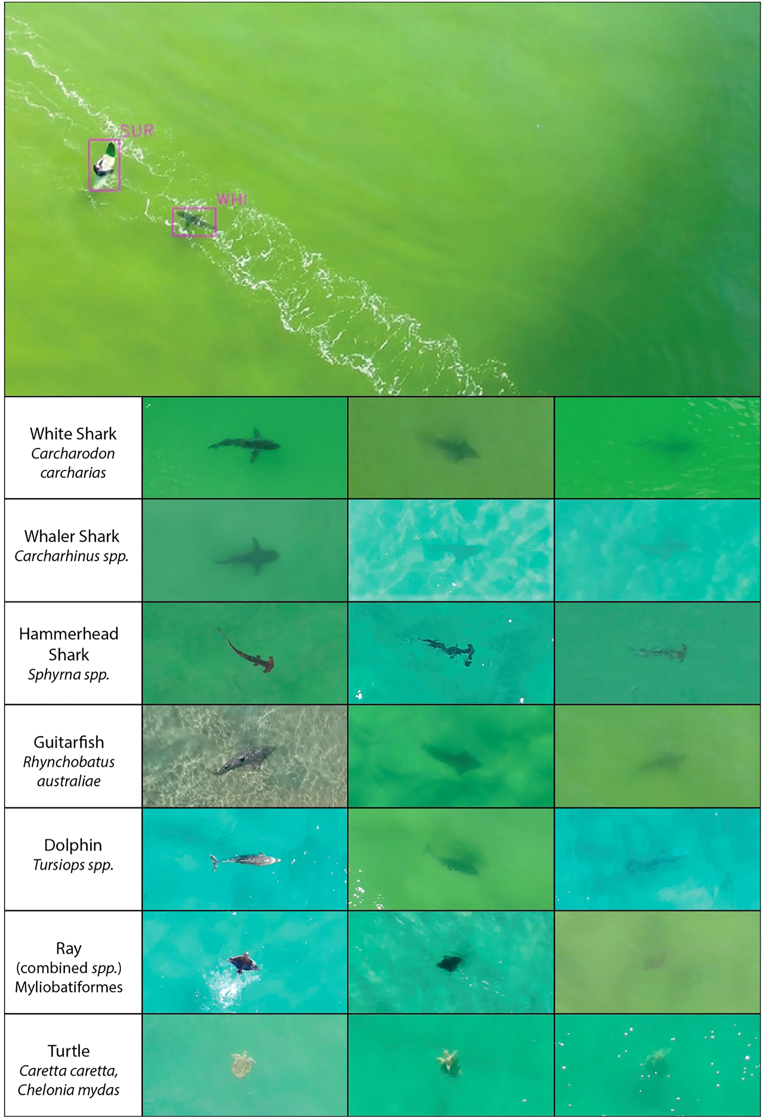
Figure 1 Examples of image data used in this work. Top Image: Representative view from the drone at a height of ~ 60m (image has been cropped from the full-frame view). Here we see a close interaction between a surfer and a white shark C. carcharias. Pink rectangles illustrate the closely-fitted bounding boxes used to train the object detection model. Lower Images: Each row presents high-, medium- and low-quality images, respectively, of the animals investigated in this study. The quality assessment was done manually by experienced observers and depends on the depth of the animal, water turbidity, sun glitter and degree of distortion at the surface.

Two subsets of video data are used in this work: (1) videos from the Phase 3 and 4 Drone Trials, recorded during 2016/2017 and (2) videos from dedicated Shark AI Trials conducted as part of this project during March-June 2020. Table 1 summarises the properties of each set of data and Figure 2 shows how objects of interest were sampled over time. At the start of this project, data from (1) were already filtered to contain only footage with positively identified fauna and hence suffer from selection bias. In contrast, videos in (2) consist of full flights recorded over many days, leading to a much more robust sample of flying conditions.

FIGURE 2

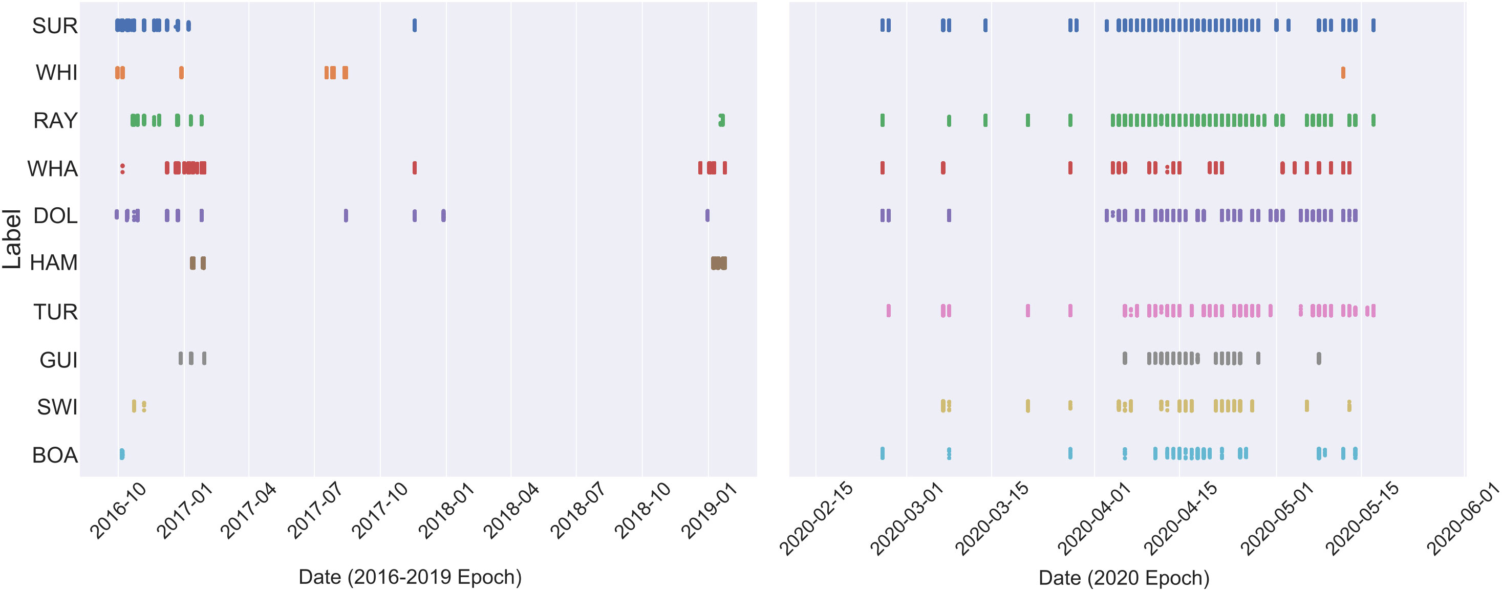
Figure 2 Illustration of the spread in dates during which objects of interested were detected. Detections during 2020 are less sparse than during 2016/2017/2019 as the 2020 trials were designed with training and validation of the machine learning algorithms in mind. Each object class is represented as a three letter code as follows: SUR, surfer; RAY, ray; WHI, white shark; WHA, whaler shark; DOL, dolphin; HAM, hammerhead shark; TUR, turtle; GUI, guitarfish; SWI, swimmer and BOA, boat.

2.1 The phase 3 and 4 trial data

The Phase 3 and 4 Drone Trials data (hereafter P34 data) consist of 425 videos between ~ 1 and ~ 10 minutes in length. Almost all videos feature positively identified marine fauna in addition to beach users (e.g., surfers, swimmers) and marine equipment (e.g., boats, jet-skis, buoys). These videos were clipped from original recordings of full flights and are highly biased to select for environmental conditions where animals were visible and identifiable to experts. This means that only a small fraction of video frames are empty of objects. Importantly, the P34 data does not represent the full range of scenes encountered over the course of normal flying. Examples of confusing objects and features (e.g., seaweed, reef, rocks, surf-wash, brackish water) are essential to train the ML model what not to pay attention to. Without sufficient negative examples, ML models trained from only the P34 data will have a very high rate of false positives when deployed in the field; that is, the models will fail to generalise.

2.2 The shark AI trial data

Dedicated trials of a prototype mobile shark detection application were conducted during February-May 2020. These trials, run in partnership with SLS NSW, provided essential coverage of confusing objects and recorded a wide range of environmental conditions, which will help models to perform better in all weathers. They also added significant examples of rare species to increase the sampling of minority classes.

The data consist of full-flight videos taken at five beach locations by SLS NSW pilots, adding up to 149 days of flying in aggregate (see Table 1). Videos of each flight were recorded onto on-board memory and the live 1080p video telemetry was processed using the prototype Android Shark AI App that applied a neural network based object detection model in real time (see § 6 for details). From April 15^th 2020 onward the application automatically logged all detections made by the model for later offline comparison. A summary of each flight was also created by the SLS NSW pilots on a paper flight-sheet and electronically recorded in their flight management system.

TABLE 1

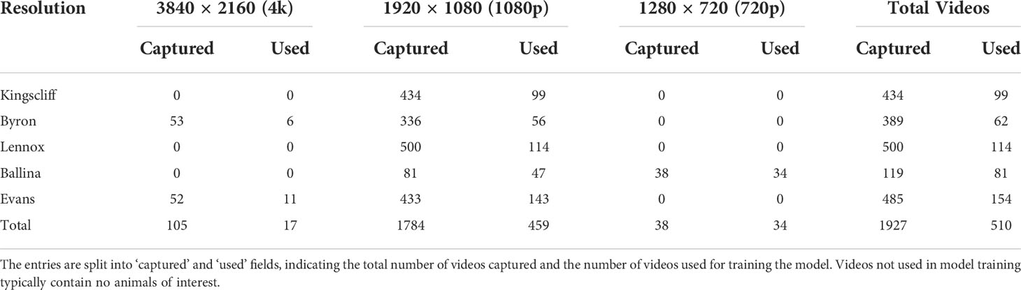
Table 1 Summary of the number of videos, their capture locations and capture resolution for the Shark AI Trial data used in this work.

3 Preparing the data for machine learning

Data preparation is a critical step in creating a robust machine learning workflow - one that is often neglected in the established literature in favour of covering algorithmic innovations. However, the programming maxim ‘garbage in: garbage out’ applies equally to machine learning, and necessary data preparation can consume in the of order 90% of the effort dedicated to a project. Operations on the data include: data exploration and visualisation, quality control, labelling, correcting for missing values, normalisation, de-biasing and correcting for in inhomogeneous sampling.

3.1 Labelling the data

This project uses supervised learning techniques to detect and identify objects in each video frame. Hence, the training data must include rectangular bounding boxes, marking the spatial extent of objects of interest and their identifier label. Creating such labels is a labour-intensive process, requiring the close supervision of a shark expert, so we employed the following iterative procedure to speed up the process.

1. Play each video forward and use the mouse cursor to manually follow fauna with a rectangular aperture. The size and aspect ratio of the aperture can be changed via the keyboard, resulting in time-series ‘tracks’ of closely-fitted boxes that are saved to disk in JSON format alongside each video. Each track has an associated label indicating object type (e.g., whaler shark, surfer etc.) and a quality flag in the range 1 – 5.

2. Apply an object-detection model in inference mode to automatically generate tracks (if a suitable model exists). This step can be performed in lieu of (1) when the performance of the model from (6) reaches a suitable level. This greatly speeds-up the labelling of new videos.

3. Visualise and edit tracks of bounding boxes for each video using a graphical user interface (GUI). We developed the custom Shark AI GUI that supports a wide range of labelling operations, including drawing new bounding boxes, interpolating between key boxes to create new tracks and labelling negative images - frames that contain no objects of interest.

4. Extract a sample of JPEG-format full-frame images from the labelled videos and create an adjacent ASCII comma-separated-variable (CSV) file to hold the coordinates and labels of the bounding boxes. This is the basic ML-ready dataset that can be used to train an object detection algorithm.

5. Apply image augmentation, normalisation and over-sampling, as described in §3.3.

6. Train an object-detection model to detect and localise objects in new video data (see §4).

The initial models were created using a small set of labelled data generated by step (1) above. As more data were added to the training loop, the model accuracy increased and false-positive rate decreased so that step (1) could be skipped entirely and the model used to generate new labels in (2). Early efforts displayed many artefacts, so the graphical labelling tool (3) was essential to edit the tracks and correct any mistakes. Over time, this iterative process converges towards a best-performing model.

3.2 Data biases and generalisation

Neural networks suffer from many of the same issues as simple curve-fitting algorithms. Chief amongst these is the issue of overfitting or generalisation: does the best fit to the training data describe new data encountered in the real world? If the answer is ‘yes’, then the model generalises well. But if the answer is ‘no’, then the model is likely to suffer from overfitting, where the model will do a good job of predicting new data with very similar characteristics as the training data, but will perform poorly for completely new data. It is common practice to split off a fraction (e.g., 5 –10%) of training data into a test set, which is then used to assess the performance of the trained algorithm. Gauging performance using the test set provides a measure of how well the neural network has learned features in the data that correspond to each class. However, if the training data do not sample the full range of conditions encountered in the field, then the real-world performance will be worse than testing indicates. In other words the best fit model will not generalise well to new data.

Of particular concern are systematic differences between classes that do not relate to the unique features of individual object types. Such biases are a common problem for data collected on rare objects, leading to ensemble properties that may be highly skewed compared to the median. For example, in the current dataset hammerhead sharks are present mostly on sunny days and in clear water. Hence, most training images of hammerheads are dominated by pixels representing bright green sea. Without correcting for this class-level bias the machine learning algorithm would associate the hammerhead label with dark objects on a bright green background, rather than just picking out the distinctive shape of the shark. To mitigate against these sorts of problems, we must normalise the distributions of each property that we do not want the algorithm to learn from - in this example the background colour of the images. We note that our data are well suited to this type of colour correction because typical images are dominated by the ocean and most scenes are relatively simple and uncluttered.

3.3 Normalising data distributions

The key to training a robust, accurate and unbiased classifier is a large and statistically balanced training dataset with accurate and appropriate labels. No real-world dataset is perfect, so we use a number of techniques here to mitigate against problems in the data and make incorporating new data as easy as possible. In particular, we measure the distributions of size and colour within each object class and apply transformations to shift their properties closer to target distributions.

A number of methods exist in the statistical literature to transform non-normal distributions to Gaussian form (e.g., Draper, 1952; Box and Cox, 1964; Gasser et al., 1982; Chen and Tung, 2003). However van Albada and Robinson (2018) recently presented a transformation that outperforms the previous methods, is exceptionally easy to implement and minimises the required shift for each datum. The method works by sorting the data into a cumulative distribution function (CDF) and shifting each data point onto the equivalent curve for the target normal distribution. For a variable v following a continuous distribution, Equation 8 of that paper states

$\begin{array}{ll}y(v)=\mu +\sigma \sqrt{2}\text{ er}{\text{f}}^{-1}[2P(v)-1]& (1)\end{array}$

where P(v) is the CDF of the data, erf^-1 is the inverse Gaussian error function, μ is the mean of the target normal distribution and σ is the standard deviation. The application of Equation 1 is illustrated in Figure 3 which shows the shift applied to each datum in a bimodal distribution in order to normalise it. In practice, the magnitude of the allowed shift should often be limited (e.g., only positive values allowed for certain parameters), so data that are shifted outside set limits are randomly shifted again to fall within the distribution. If a very narrow clipping range is applied, this can result in the distribution sitting on a ‘pedestal’, but this has not been an issue for any transformations applied in this work.

FIGURE 3

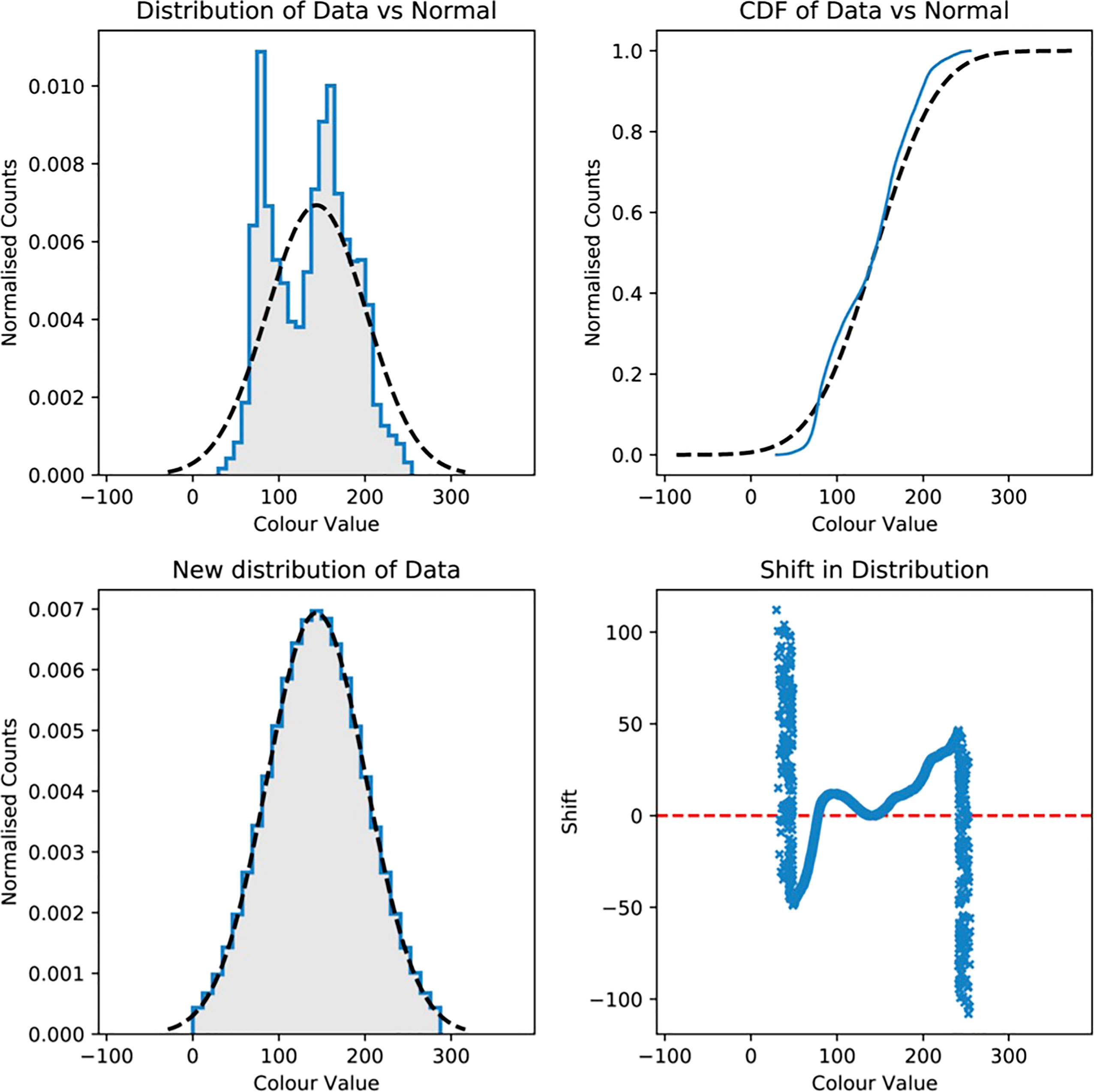
Figure 3 Illustration of how a non-normal distribution is transformed to Gaussian form via Equation 1. The top-left panel shows the distribution of raw data (shaded histogram, in this case ‘colour value’) overlaid by a normal distribution (dotted line) with similar values for median μ and standard deviation σ. The equivalent cumulative distribution functions (CDFs) are shown in the top-right panel. The bottom-right panel presents the shift necessary to transform each value onto the target normal distribution. Note that the vertical spikes present on left and right of the shift curve are due to clipping at ±2.5 σ. The final distribution is shown in the bottom-left panel and corresponds well to the Gaussian curve, despite the clipped values.

3.3.1 Mitigating colour biases

The largest biases in the DPI Drone Trials Dataset are due to differences in the ‘background’ sea colour, linked to variations in environmental conditions between data acquisition flights. We also know that shape (rather than colour) plays a dominant role in distinguishing between shark species, as most sharks have similarly coloured skin. Hence, we normalise the colour distributions between classes, effectively forcing the neural network to pay less attention to colour differences and instead focus on learning shapes and textures in the training images.

We perform colour normalisation on the training images with colours encoded as hue, saturation and value (HSV). Hue varies between 0°→360° with a smooth transition at the wrapping point, which allows us to shift the hue distributions without introducing discontinuities. In practise, all training images are loaded for a particular class, converted to HSV encoding and robust statistics (e.g., MADFM) are used to measure their median HSV values. Equation 1 is used to calculate the normalisation shift for each image, which is then applied before the images are written back to disk in RGB format.

3.3.2 Mitigating size biases

Individual classes of object have characteristic size distributions that differ significantly from each other. However, the observed size is a strong function of the altitude of the drone and we want the detection system to perform equally well at low (~10 m) and high (~60 m) altitudes. For this reason, we scale, crop and resize input images to achieve a more balanced distribution of object sizes across all classes. In the same way as the colour correction operation, we measure the distribution of ground-truth box sizes, set a target distribution based on the median size and calculate a ‘zoom factor’ for each image that defines the scale and crop to be applied. In crowded frames we invariably crop out some labelled objects, however, we minimise the number of dropped objects by carefully selecting the location of the zoomed frame bounds. We are also careful not to scale the image data by more than a factor of 3 ×, which would result in very blurry images. During this operation we also apply a random rotation in multiples of 90°, which mitigates against a tendency of pilots to follow fauna from the rear, meaning that the majority of sharks are filmed swimming facing ‘up’ in the video footage.

3.4 Properties of the labelled data

Here we present the properties of the labelled training data. In total, we created 3501 tracks (time-series of a single bounding box) in 712 individual video files. Figure 4 presents a histogram of the labelled data broken down by species and location. The number of boxes labelled in each class varies dramatically, with boats and swimmers having the least samples and surfers and rays the most. Guitarfish, hammerhead sharks and turtles are undersampled compared to the other fauna, and samples are drawn from only a few independent videos of each. It is notable that most white shark video data was sourced from Colefax et al. (2020a), which were from separate locations to the rest of the dataset.

FIGURE 4

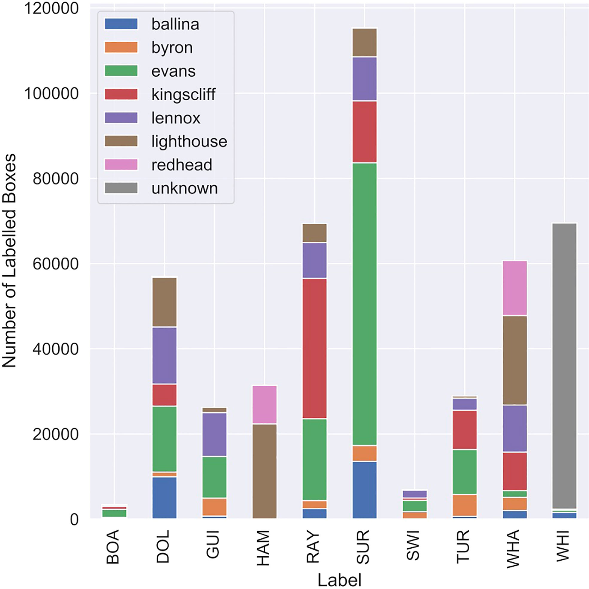
Figure 4 Distribution of sampled bounding boxes over the ten classes of interest, divided by sampling location.

Figure 5 shows the distributions of HSV colours for all training images in the ten object classes and the effect of the colour normalisation process. Taking hue as an example, before normalisation most distributions are centred around a hue H = 0.4 corresponding to the green appearance of sea water from the air, however, the shapes of the distribution vary considerably. The distribution for white sharks (WHI) is very narrow, likely representing a bias towards particular weather conditions. After normalisation, the distributions of colour hue in most classes appear similar with an approximately Gaussian profile. However, the colour differences for surfers and swimmers are genuinely different because they are often seen towards foamy water, therefore we only smooth the distributions for these classes (rather than shift).

The distributions of colour saturation (middle panel of Figure 5) were adjusted to broadly sample the full gamut of values 0 - 1. The most extreme adjustment was applied to white sharks which exhibited a narrow distribution of saturation values peaking at S ≈ 0.86, prior to normalisation.

FIGURE 5

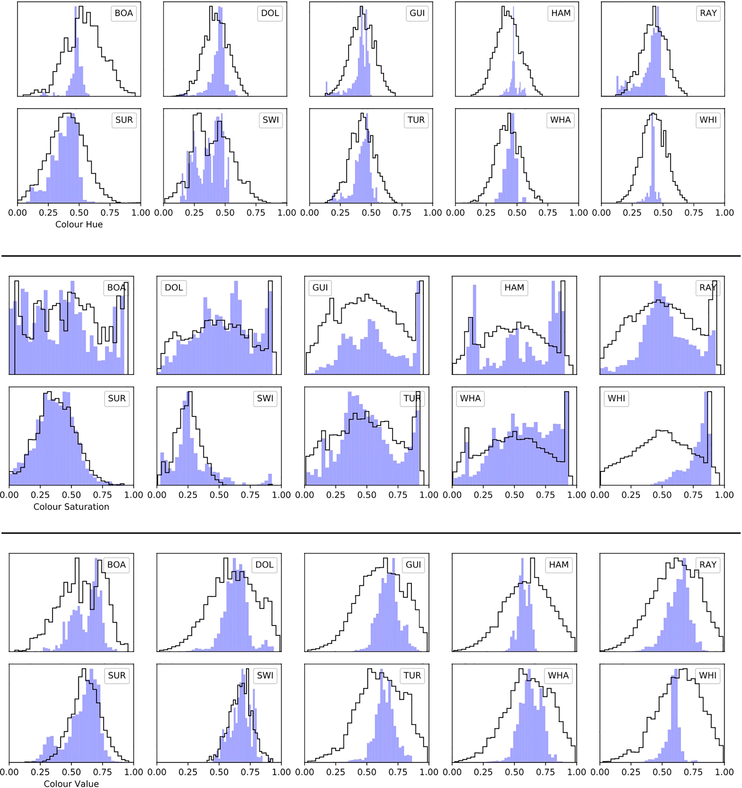
Figure 5 Distributions of median colour hue (top), colour saturation (middle) and colour value (bottom) for training images in all ten classes. Hue values cluster near to H ≈ 0.4, which encodes the average colour of the sea as green. Colour value and saturation encode brightness and colour intensity, respectively. In each panel the blue-filled histogram shows the distribution before normalisation, while the black outline histogram shows the distribution after applying the colour normalisation scheme described in § 3.3. After normalisation, colours are more similar between classes and sample a larger range of parameter space.

The distributions of colour values (encoding brightness) were broadened to better sample a range of lighting conditions. Again, the exceptions were the ‘surfer’ and ‘swimmer’ classes, which we only smoothed as they tended to occur in bright foamy water.

Figure 6 top presents the distributions of bounding box geometric size $(\sqrt{height\times width})$. There is considerable variation between classes, some of which derives from the natural size of different object types (e.g., turtles are smaller than boats) and some from biases within the data. Hammerhead and white sharks in particular have long tails of very large bounding boxes. This feature derives from an over-representation of videos where the pilots zoomed in on the animal so that it filled the frame. We attempted to normalise the distributions of sizes as outlined in §3.3.2, but were limited by the large tranche of low-resolution (1080p) training data from the 2020 trials that cannot be resized without degrading quality significantly. The overlaid unfilled histograms in Figure 6 shows the final size distributions for the training data. Note also that images containing large bounding boxes cannot be cropped, so that skewed distributions of hammerhead and white shark sizes remain largely unchanged.

FIGURE 6

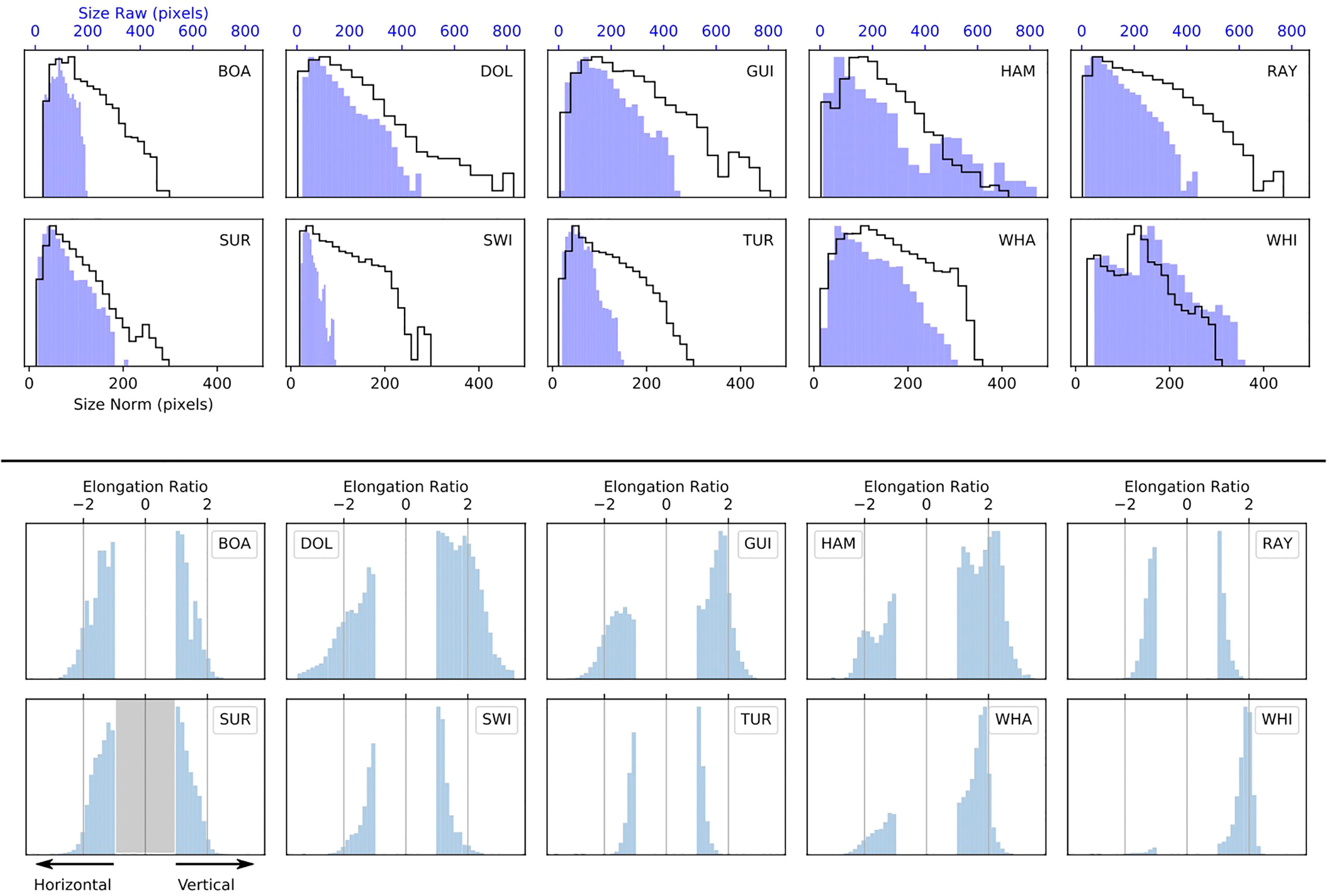
Figure 6 Top: Histograms showing the distributions of bounding box size for each class of object on a log scale (y-axis) to emphasize the low-level structure. Here ‘size’ is the geometric average of the side-lengths √ height × width. In each panel the blue-filled histogram shows the distribution before normalisation, while the black outline histogram shows the distribution after applying the scaling and cropping scheme described in § 3.3.2. This offline augmentation technique attempts to normalise the size distributions between classes by cutting out a zoomed section of image, but this method cannot be used when objects occupy most of the frame, as is the case for significant numbers of hammerhead and white shark images (labelled HAM and WHI above). Note the different x-axis scales for the ‘before’ and ‘after’ distributions, reflecting the down-sizing of training images to 1080p resolution. Bottom: Distributions of bounding box elongation ratio for each class in the training data after augmentation. Vertically elongated boxes have positive ratios (= height/width) and horizontally elongated boxes have negative ratios (= −1×width/height). Note that boxes around white sharks (WHI) are almost all vertically elongated, indicating animals tracked from behind by the drone operator. There was limited scope to rotate these data because many animals occupied the full field-of-view. Whaler sharks (WHA) and guitarfish (GUI) also show similar issues, but to a less extreme degree. Turtles (TUR) and rays (RAY) tend to have ratios closer to unity, indicating more square boxes.

Finally, Figure 6 bottom plots the distributions of bounding box elongation ratio after data normalisation. Boxes elongated in the horizontal direction are assigned negative values to distinguish them from vertically elongated boxes. Almost all of the large targeted animals (dolphins, guitarfish, hammerhead sharks, whaler sharks and white sharks) exhibit distributions skewed towards the vertical because we could not adequately correct the ‘rear filming’ bias described earlier.

4 The object detector and training pipeline

Two versions of the pipeline exist with identical steps, differing primarily in the architecture of the backbone neural network used. We train two RetinaNet single-shot detector (SSD) models (Lin et al., 2017) with backbone classifier networks based on the ResNet-50 and MobileNet V1.0 architectures. ResNet-50 is a deeper network than MobileNet V1, more suitable for deployment on a high-powered mobile device (e.g., an iPad Pro) or a GPU-accelerated desktop computer. MobileNet V1 is a shallower architecture, specifically designed for deployment on devices with limited processing power and lacking hardware to accelerate machine learning (e.g., phones or tablets with older processors).

Our choice of RetinaNet and these two backbone networks is motivated by deeply practical reasons. These algorithms are well-characterised, offered ‘good enough’ performance in other applications and were in widespread use during 2018 - 2020, when most of this research was conducted. In addition, the combination of a SSD with Mobilenet V1 was supported by a deployment tool-chain targeting Android devices. This was critically important for developing and field-testing our proof-of-concept mobile application.

It is also widely acknowledged (e.g., Mazumder et al., 2022) that more research is needed on curating high-quality datasets to support the development of models that perform well when deployed. We emphasise that the focus of this work is on the data, rather than algorithms.

4.1 RetinaNet

RetinaNet was developed by Lin et al. (2017) to address the common problem in SSDs of the ‘background’ (empty) class dominating the training. This happens because the detector samples a large set of candidate object locations across each image, most of which contain nothing of interest. RetinaNet uses a novel loss function - called Focal Loss - to down-weight these easily learned examples and allow training to a high-accuracy. The detector also implements a laterally-linked feature pyramid for detecting objects at different scales. Even in 2022, RetinaNet is considered a reasonable choice for a high-performing object detector: versatile enough for deployment on a mobile device and accurate enough to approach the best multi-stage detectors (e.g., Pyrrö et al., 2021). We use two implementations of RetinaNet for this work: for the ResNet-50 architecture we employ an open-source Keras-based code developed by robotics company Fizyr³, while for the MobileNet V1 architecture we use the implementation in the TensorFlow 1.5 Object Detection (TFOD) API⁴.

4.2 The training pipeline

The training pipeline is configured to run isolated experiments that feature different data sampling schemes and training hyperparameters. Labelling, image-extraction and augmentation tasks are run in the first part of the pipeline, to produce a static dataset of normalised 1080p resolution images with bounding boxes (for details see 3.3). This is the fundamental dataset that experiments draw on. A subset of the data is then prepared for an experimental training run. Steps include:

● Clipping the maximum number of boxes in each object class.

● Oversampling minority classes via random replication while taking care that images containing multiple classes of object are fully annotated.

● Splitting out separate training and internal validation sets.

● Filtering for a subset of object classes and merging object classes into new or existing labels.

As previously shown in Figure 4, some classes are under-represented leading to significant imbalance in the dataset. This is a natural consequence of the rarity of some animals and because the locations are unevenly sampled. Such imbalance can be mitigated in a number of ways: by targeting a metric other than accuracy while training; by weighting the loss function with the inverse occupancy for each class; or by re-sampling the data. Here we choose to oversample minority classes by randomly replicating data - early experiments suggested that this is equivalent to the weighting the loss function. Many of the ocean scenes contained multiple species, meaning that care was needed to avoid over-representing some classes when replicating another. Images to be replicated were drawn from the subset that contained no other species and replication was only attempted if 70% of the images contained boxes for that class alone (true in most cases). This procedure allowed us to maximise the information content, while balancing the classes in each training set and avoiding excessive data repetition. The models were trained using a target of 20,000 boxes per class and two percent of data was randomly split off before the oversampling step, to serve as an unseen internal validation set. Once chosen, the training and validation data were randomly shuffled and written to disk in the experiment directory.

The remainder of the training workflow is standard for this type of problem. Randomised mini-batches of annotated images were run through the network in a forward-pass and the loss calculated. The weights between layers were tweaked in the back-propagation pass and this training loop was repeated until the loss plateaued, or a maximum number of epochs was reached. A snapshot of the weights were saved to the experiment directory after each epoch. The best fitting model was chosen by examining the loss and mean average precision (mAP) curves and selecting the epoch where the curve had just flattened.

Training hyperparameters, such as learning rate, were tweaked manually until satisfactory results were obtained. Lower learning rates (~ 0.001) and longer training times tended to produce the best results. Although we did not have the computational resources to do a more comprehensive search of hyperparameter space, we believe the results are close to optimal for our training setup.

Due to limitations in the TensorFlow implementation, the MobileNet V1 model was configured to read in an image tensor of [w, h] = [800,480] during training, rather than [1920,1080] for the ResNet-⁵0 backbone. However, during testing both networks performed inference on 1080p resolution images, which was possible because of their fully convolutional architecture.

5 Results and analysis

The primary aim of this work is to assess how well a modern neural network based object detector performs at distinguishing shark species. The results presented here constitute a baseline for comparison with future algorithmic advances. Equally, the properties of the current dataset impose limits on detector performance and we investigate enhancements to the input data that are required to make a truly robust shark detection model.

5.1 Assessing model performance

We assess the performance of the trained object detector by running the model in inference mode on unseen test data. Three main variables affect the model performance at inference time:

1. The non-maximum-suppression (NMS) threshold: this is the value of intersection-over-union (IoU) IoU_NMS above which boxes in the same frame are considered duplicates.

2. The confidence threshold s ≥ s_thresh at which to accept candidate detections.

3. The IoU threshold (IoU_match) used to match detected and ground-truth boxes.

At the lowest level, the object detection algorithm produces a list of candidate bounding boxes generated by the model at anchor points across each image frame. Each box has an associated label (e.g., HAM, WHI, SUR etc.) and confidence score s in the range 0 - 1. Boxes are grouped into clusters by calculating the IoU between pairs of boxes - this is the ratio of intersecting to unified area. IoU values range from zero (no overlap) to one (perfect overlap) and boxes are considered part of a cluster above a threshold IoU value. During the NMS operation, only the box with the highest confidence score within a cluster is retained and the others are discarded. Our experiments show that a threshold of IoU_NMS = 0.3 works well for our dataset.

Figure 7 shows how the average recall of the model varies with IoU_match threshold. We see here that recall is not strongly dependent on IoU_match between values of 0.1 and 0.4. In practice, we choose a value of 0.3 for IoU threshold to measure performance of models and compare between models.

FIGURE 7

Figure 7 Plot of Recall ( = True Positives All Detections ) versus IoUmatch threshold used to cross-match detections with ground-truth annotations. The curve shows that recall remains reasonably stable over a range of IoUmatch thresholds from 0.1 to 0.4.

After the NMS step, the list of detections are cross-matched with the ground-truth boxes via another IoU operation and the following three catagories are defined:

● True Positive (TP): detections with confidence scores s ≥ s_thresh, that overlap a ground-truth box with IoU ≥ IoU_match and have the same class label.

● False Positive (FP): any detection that does not meet the above criteria.

● False Negative (FN): a ground-truth box that is not matched with a detection.

A distinction can be made within the FP class between correctly localised objects that are assigned the wrong label and entirely spurious detections. The results are used to build a confusion matrix, plot precision-recall curves and calculate the average precision for each class of object, and the mean average precision (mAP) for the detector. In constructing these metrics, we follow the method of Padilla et al. (2021), who reviewed object detection metrics in common use and provided excellent reference code⁵.

5.1.1 Testing data

We test models against two distinct types of dataset:

1. Internal data randomly split from the same pool that the training data was drawn from.

2. External data deliberately chosen from different locations, or significantly different times, or both.

Each of these datasets addresses different questions. The internal data (1) asks the question ‘How well has the model learned the differentiating features between object types in the training data?’. However, caution is needed here as some of these learned features may reflect biases, or correlations, in the data, rather than the distinguishing features of target objects. Weather and illumination change are often stable over the course of a flight, meaning that testing and training images drawn from the same videos will likely sample similar conditions. This correlation in conditions will manifest as artificially high performance scores.

A more realistic test is offered by the external data (2), which poses the question ‘How well does the model cope with unseen data, at new times and/or locations?’ Because the data is separated in location or time, it is much less likely that significant correlations will occur. Testing against these data shows how the model would likely generalise to new environments, without further tuning.

5.2 Performance of ResNet-50

In this section we present detailed performance analysis of the model architecture with the ResNet-50 backbone. Our investigations in § 5.4 later illuminate properties of the data that lead to performance limitations in the model.

5.2.1 Performance on the internal data

We first measured the performance of the trained model by testing against the internal validation data. Figure 8 presents three confusion matrices created at confidence thresholds s_thresh = 0.1, 0.5 and 0.9, along with precision-recall curves for each class of object.

Confusion matrices are a valuable diagnostic tool, pointing to how and why a detector might be producing a particular result. The matrix for a model with perfect recall would have a diagonal where all values are 100%, meaning that all ground-truth boxes for each class are detected and identified with the correct label. Indeed, the matrix for s_thresh = 0.5 (bottom-left) displays excellent performance: well above 90% of objects are correctly detected for most classes. The row for rays (RAY), for example, has non-zero off-diagonal elements, indicating correctly localised objects with incorrectly predicted labels. In this case 2% of rays are incorrectly predicted to be turtles (TUR).

Our confusion matrices also have an extra row and column appended to them. The bottom row is used to encode entirely spurious false-positive detections, while the rightmost column records ground-truth boxes that were not detected (false-negatives). At a low confidence acceptance threshold of s_thresh = 0.1 (top-left in Figure 8 many spurious detections (false-positives) are accepted and the bottom row of the matrix has significant non-zero elements. Conversely, at a conservative confidence threshold of s_thresh = 0.9, most candidates are rejected, leading to high percentages of false-negative values in the last column of the matrix (top-right in Figure 8). Dolphins and swimmers have the highest values here, indicating that the predicted confidence value for these classes most often falls below 90% (i.e., the object detector is most uncertain about these classes).

FIGURE 8

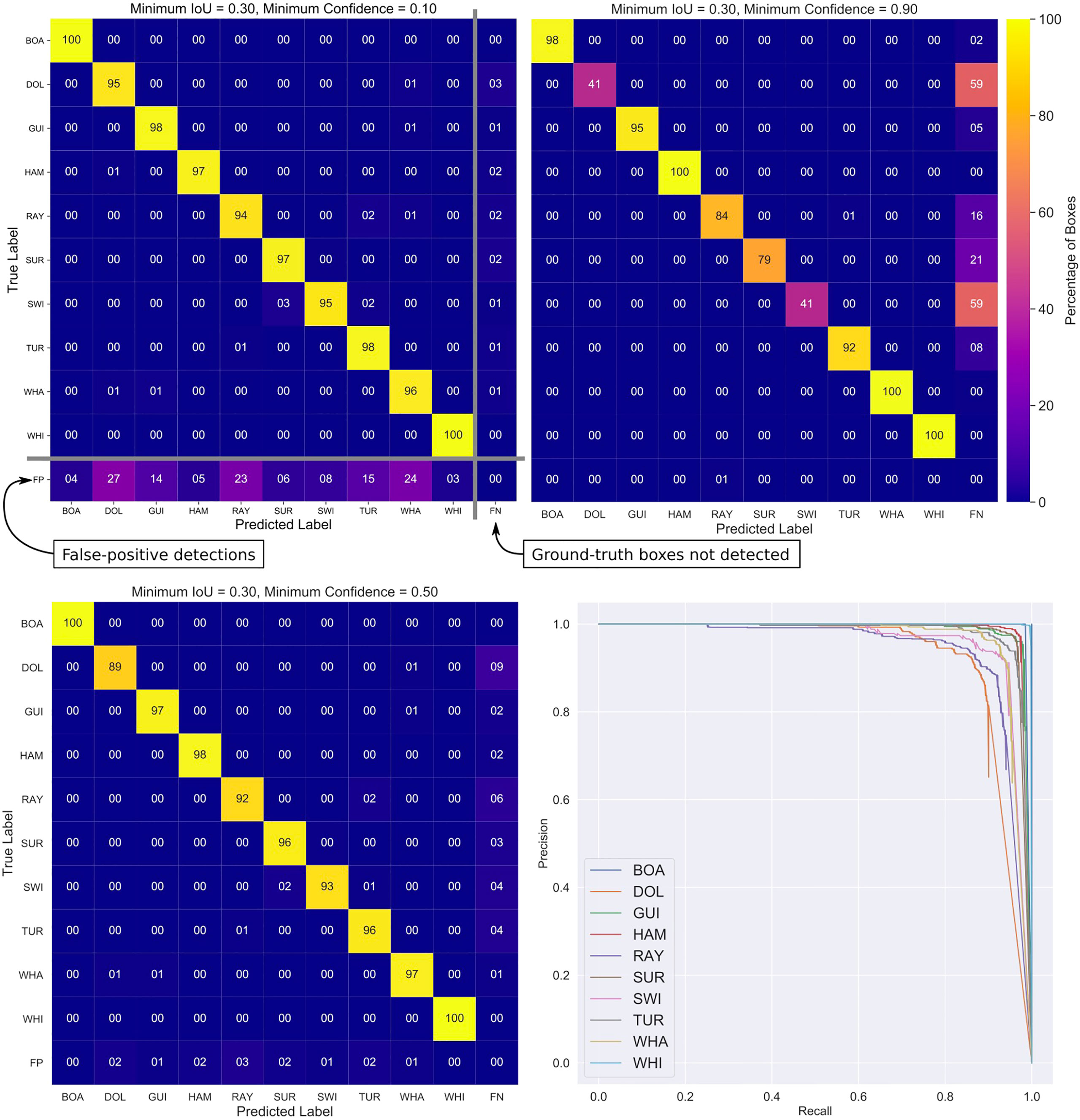
Figure 8 Top row & bottom-left panel: Three confusion matrices for the final ResNet-50 backbone model created at confidence score thresholds of 0.1, 0.5 and 0.9. A common IoU threshold of 0.3 was used to cross-match ground-truth and detection boxes. The model was tested against an unseen internal test set randomly split from the ensemble data. Each row in the matrix encodes how ground-truth labels (y-axis) were predicted by the classifier (x-axis). The prominent diagonal shows that most objects were detected and labelled correctly. Off-diagonal elements show when a particular class is mislabeled as another - an important diagnostic of why a model is failing. The bottom row of the matrix encodes false-positive (spurious) detections, which are common when the score threshold is low. Note that the bottom row can have percentages greater than 100, meaning that there are greater numbers of false-positives than ground-truth boxes. The right-most column shows false negative detections - real objects that were missed by the algorithm. These are common when the confidence threshold is high as the model rejects a high fraction of candidates. All rows, except FP, add to 100 percent. The mean average precision for the best fitting model is mAP = 0.96. Bottom-right panel: Precision-Recall curves broken down by class. The area under each curve gives the average precision for each class.

The bottom-right panel of Figure 8 presents the precision-recall curves for each class. For object detectors the area under the curve (AOC) is equal to the average precision (AP), which can be used to directly compare performance between models and classes. The mean average precision for the ResNet-50 model on the internal testing data is mAP = 96%.

5.2.2 Performance on the external data

The external data presents much more of a challenge to the trained model. Videos in this dataset were sourced from the same locations, but at well-separated times (Byron, Ballina, Evans and Lennox beaches during late 2017), or from completely new locations (Forester, Broken Head, Angourie beaches and South-West Rocks, during 2017/2018). Because the data sample different conditions and environments, the results of tests here will be much more representative of performance in the field.

We measured the performance of our final trained model against the external data and Figure 9 presents the confusion matrix at s_thresh = 0.5 alongside the precision-recall curves. It is immediately apparent that the performance on the external data is worse - as expected. We still see a clear diagonal indicating reasonable overall performance and the mAP for the model is 51%, representing a fall of 45%. However, the degradation in performance is not uniformly spread across object types. The worst performing fauna here are the guitarfish, where 42% of ground-truth boxes are misclassified as whaler sharks and 19% vice-versa. Interestingly, whaler and white sharks are often confused for each other, with 53% of white sharks classified as whalers and 16% of whalers classified as whites. Also, 27% of hammerhead shark boxes are confused for whalers. Note that if we combined the whaler, white and hammerhead classes into a single ‘dangerous shark’ class, 80% of boxes would be correctly detected and labeled. We also see a large number of false-positive identifications of white sharks at 25%. In the human object categories, the performance of the model correctly detecting swimmers is very poor with 59% being misclassified as surfers and 21% not detected at all.

FIGURE 9

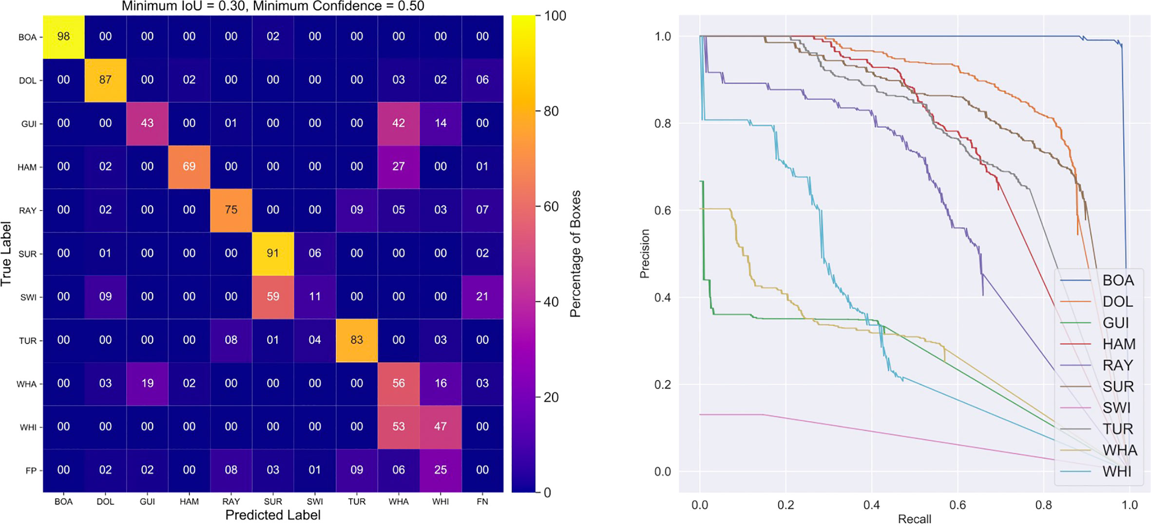
Figure 9 Confusion matrix (left) and precision-recall plot (right) for the final ResNet-50 backbone model applied to the external testing dataset. The cross-matching IoU threshold was set at 0.3 and confidence score thresholds at 0.5 for optimum performance. The external data presents a harder and more realistic challenge compared to the internal data, as indicated by the mean average precision falling to mAP = 0.51. However, the performance is still reasonable when seeking to distinguish between sharks and other objects. Some general patterns are visible: swimmers are confused for surfers and white sharks for whalers over half of the time. Guitarfish are misidentified as whaler sharks 42% of the time, but much less often the other way around (19%). Hammerheads are also sometimes confused as whalers, and swimmers are occasionally not detected (21%). Analysis reveals that most of these issues are explained by biases in the training data, or systematic differences compared to the testing data.

5.3 Performance of MobileNet V1

Here we report the performance of the model based on the MobileNet V1 network architecture. Note that the version of the model deployed to the mobile device is compressed by decreasing the floating-point precision at which the neuron weights and activations are recorded. We find that this operation has no significant effect on accuracy and the following assessment has been done on a desktop-class GPU, so a direct comparison can be made with the ResNet-50 backbone network.

5.3.1 Performance on the internal data

Figure 10 presents the confusion matrix and precision-recall plot for the final MobileNet V1 model applied to the internal testing data. Overall, the performance approaches the larger ResNet-50 model, with a mAP of 93%, compared to 96%. The major difference visible in the right-most column is that the MobileNet V1 model produces more false negatives - real objects not detected. Interestingly, surfers, swimmers and dolphins are missed most often.

FIGURE 10

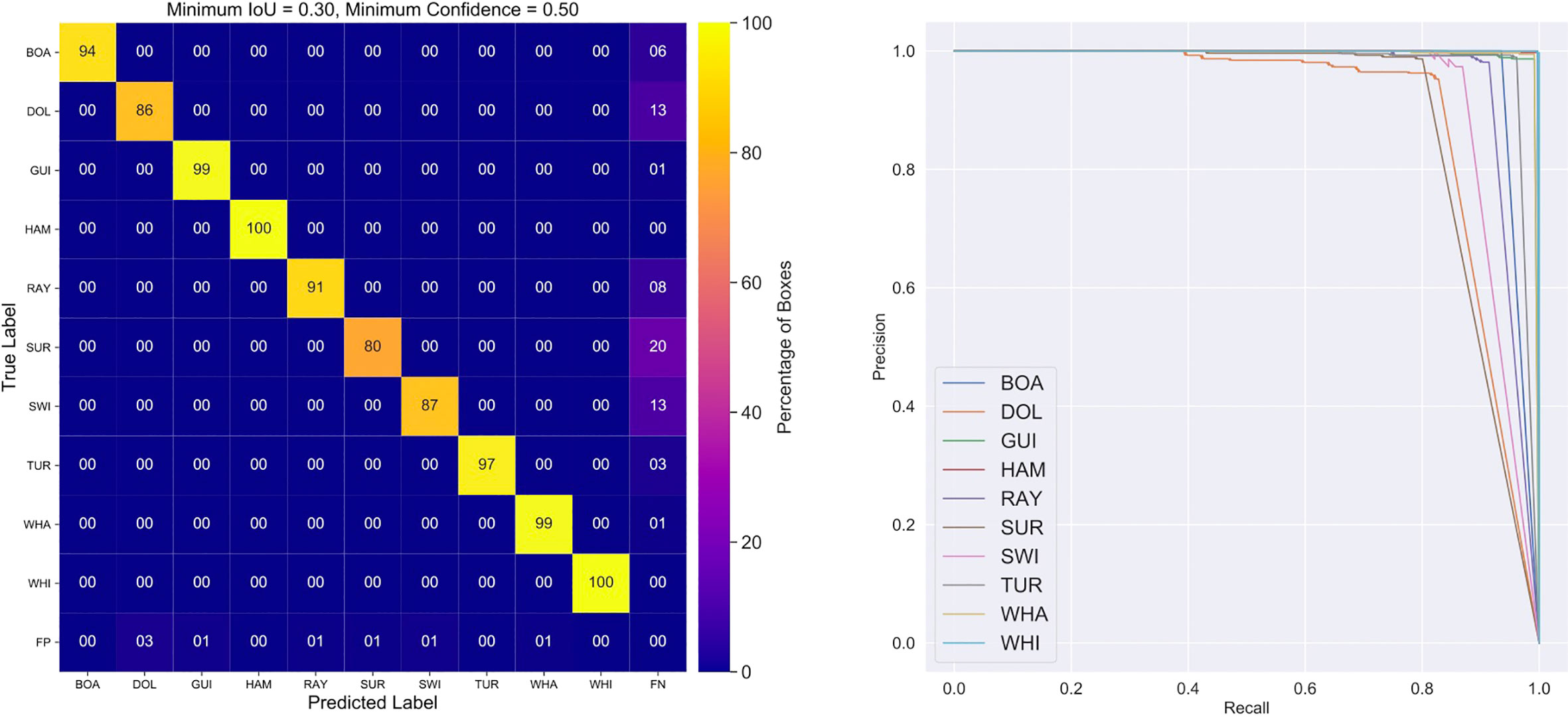
Figure 10 Confusion matrix (left) and precision-recall plot (right) for the final MobileNet V1 backbone model applied to the internal testing dataset. The MobileNet V1 architecture performs similarly to RetinaNet 50, despite being more lightweight. Comparing this confusion matrix to Figure 8, we see that the MobileNet V1 model exhibits a few more false negatives (real objects not detected) in the rightmost column. However, taken as a whole, the network performs well on identifying dangerous shark species, with a mAP = 0.93.

5.3.2 Performance on the external data

As expected, testing the MobileNet V1 model on the demanding external dataset shows worse performance over the internal data, with a mAP = 60%. However, this value is better than the measured value for the ResNet model (mAP = 51%). Most of the same error patterns are present in the matrix: confusion of white sharks for whalers, 83% of swimmers misidentified as surfers and a quarter of whaler sharks as guitarfish. However, only 13% of guitarfish are erroneously classified as whalers and the performance on hammerhead sharks is 9% better than the ResNet-50 model. Again we see larger percentages of completely undetected objects, appearing in the right-most column. Rays are the dominant group here, with the model failing to detect 36% of these animals. Dangerous sharks are detected at an accuracy of 78%, which is similar to the ResNet-50 model.

5.4 Performance error analysis

In this section we investigate possible reasons for the issues identified in §5.2 and §5.3, and highlighted in Figures 9 and 11.

FIGURE 11

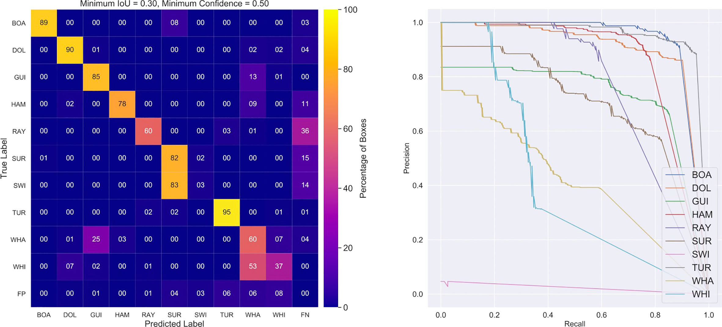
Figure 11 Confusion matrix (left) and precision-recall plot (right) for the final MobileNet V1 model applied to the external testing dataset. As expected, the measured performance is worse than on the internal dataset (see Figure 10), but still respectable, with a mAP = 0.60. Most of the same patterns are visible in the confusion matrix compared to ResNet 50 (see Figure 9), except that MobileNet V1 does less well on smaller objects (e.g., rays). Interestingly, guitarfish and hammerheads are more reliably identified compared to ResNet50, but this may reflect the longer (and slower) training regime required for the Mobilenet V1 to converge.

5.4.1 Effect of object size

Figure 12 plots the confidence score versus geometric box size for each prediction made by the best-fitting MobileNet V1 model on the external testing data. All classes follow a similar relationship of increasing confidence with larger object sizes. The detection confidence drops rapidly below sizes of ~ 55 pixels, falling beneath the acceptance threshold of s_thresh = 0.5 at a size of ~ 45 pixels. The figure also highlights correctly detected but misclassified objects, most of which are smaller than 80 pixels in size. The scatter in confidence for larger objects depends largely on data quality, which also varies between object classes. Note that object sizes are normalised to a 1920 × 1080 px image size, leading to the recommendation that objects should occupy at least 13% of the frame height for optimal performance. A similar analysis for the ResNet-50 backbone network indicates that most misclassified objects are smaller than ~ 95 pixels and the confidence drops off below ~ 30 pixels.

FIGURE 12

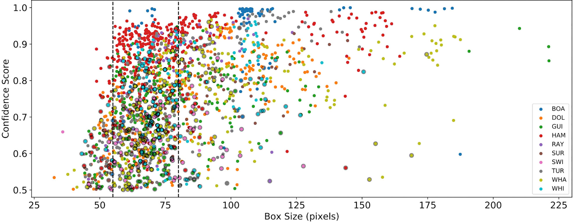
Figure 12 Plot showing the relationship between detection confidence score and object size (geometric average of the annotation box size) for the best-fitting MobileNet V1 model. Detection confidence drops rapidly below a box size of ∼ 55 pixels, falling below the confidence threshold sthresh = 0.5 at a size of ∼ 45 pixels. All classes follow a general relationship where larger objects have more confident predictions. Markers for incorrect predictions are outlined in black, illustrating that the model tends to make mistakes on objects smaller than 80 pixels in size.

The size-confidence relationship also satisfactorily explains the false-negative objects in the right-most column of the MobileNet V1 confusion matrix (Figure 11). Here, rays swimmers and surfers tend to have sizes below the 55-pixel size threshold, or are present in low-quality images (obscured, confused or blurred objects).

5.4.2 False positive detections

Although MobileNet V1 exhibits few false-positives, the ResNet-50 model shows significant numbers of spurious detections classified as white sharks. On inspection of the images, we find that they are almost all large areas of dark seaweed or submerged reef that occupy a significant fraction of the frame (Panel (a) of Figure 13 shows an example). In these cases, the issue likely derives from a bias in the current mix of training data (see §3.3.2). As shown in Figure 6, there are a disproportionate number of very large white shark boxes from extreme close-up videos taken by the drone pilots. The model has learned that the most appropriately class for large objects is ‘white shark’. This underlines the importance of carefully normalising distributions of key properties across classes in the training data.

FIGURE 13

Figure 13 Four examples of the model making incorrect predictions on the external testing data. Panel (A) illustrates two false-positives, where submerged areas of seaweed have been identified as white and whaler sharks. Spurious detections such as these are generally rare in both models and tend to appear in a single frame only. Panel (B) shows two swimmers that have been mislabelled as surfers. Active swimmers tend to have the same elongated shape as surfers, with similar features. Panel (C) shows a white shark mislabelled as a whaler shark. This happens over half of the time in both models, likely due to differences in size distribution between the training and testing data. The whaler shark in panel (D) has been mislabeled as a guitarfish due to its disturbed outline and surrounding shallow, sandy environment.

One key innovation that led to a generally low false-positive rate in or models was the deliberate inclusion of ‘negative’ images in the training data. These images contain no objects of interest and enable the neural network to learn about confounding background features, such as reefs, seaweed and rocks. Models trained before including these ‘NEG’ frames exhibited high numbers of spurious detections at beaches like Byron Bay that have complex ocean environments. The negative training images were chosen to sample a broad range of scenes and lighting conditions at each beach. During deployment, best performance will be obtained from models that are similarly ‘tuned’ to new and novel environments.

5.4.3 Incorrect label predictions

In general, both networks do very well at detecting and localising objects of interest, but sometimes fail to predict the correct labels. Further insight into the reasons for misclassifications by both models can be gained by carefully inspecting the properties of the objects that were mislabelled with the highest confidence. We visually inspected the images corresponding to off-axis diagonals in the confusion matrices when the fraction of incorrect labels was over 10% (see Figure 9 and 11) discuss the results below.

The worst-performing class in both models is swimmers, which are commonly mislabelled as surfers. All of these swimmers appear ‘stretched out’ in the water, presenting an elongated appearance that is very similar to a surfer lying on a short board (see Panel (b) of Figure 13). The model is likely identifying the ‘human shape’ features in the image to classify the detection. Swimmers are a minority class in the training data compared to surfers, meaning that adding more training images of swimmers would help mitigate this issue.

White sharks are very commonly mislabeled as whaler sharks. The images for the most confident erroneous detections show a range of qualities: white sharks with both clear and disturbed morphologies, present in a broad range of lighting conditions (see Figure 13C). However, most detections have box sizes below 70 pixels making it likely that the issues stems from the size mismatch between training and testing data. During development, this difference in size distribution was more extreme for earlier versions of our models and resulted in correspondingly worse performance: more mislabelled white sharks and greater numbers of false-positive detections. Normalising the size distribution of the white shark training data reduced both issues, but more work is needed to reach parity with other classes.

One quarter of whaler sharks are misclassified as guitarfish by the MobileNet V1 model. The worst examples show very similar characteristics to training imagery for guitarfish: turbid water, blurry or disturbed morphology and animals present in shallow water over obviously sandy sea-bed (see Panel (d) of Figure 13). Guitarfish are bottom-dwelling rays and such characteristics are an intrinsic part of their environments. Improving these detection statistics represents a significant challenge, however, guitarfish are also a minority class in the training data and adding more independent training imagery will be essential.

Finally, hammerhead sharks are sometimes identified as whaler sharks, despite their very significant morphological differences. This is a clear example of mismatch between the training and testing data. The models fail to generalise on the hammerhead class because of the small number of training images sourced from only two locations (see Figure 4). Adding more diverse training data is highly recommended.

In summary, most cases of mislabelled data have significantly different properties to the average training image, or are otherwise outliers in size or quality. The easiest solution would be to collect a larger variety of videos that can be used as part of the training data for future models. We discuss the implications of this analysis in §7, after first placing it in context by describing the mobile application and field trials conducted during February-May 2020.

6 The mobile app and field tests

To demonstrate the utility of ML-enhanced shark detector, we built a proof-of-concept mobile application that applied our MobileNet V1 model to a real-time drone video feed. The targeted deployment hardware for the app was the CrystalSky Android tablet manufactured by DJI https://www.dji.com/au/crystalsky. During 2018 - 2021 these were the dominant devices used by SLS NSW to conduct shark-spotting drone flights. The CrystalSky was chosen because of its very bright screen (2000 cd/m²), which was much preferred for viewing in the sunlit⁶ conditions often encountered on Australian beaches. However, these tablets have a relatively slow processor and run a very old version of Android (V 5.0, released in November 2014). The newer DJI SmartController⁷, also deployed by SLS NSW, presents only a modest speed increase and an update of the operating system to Android V 7.0. Both devices lack hardware or software acceleration for machine learning inference, making deployment of even the lightweight MobileNet V1 model challenging.

6.1 Design of the mobile app

The DJI Mavic 2 Enterprise⁸ drones deployed by SLS NSW can be flown using just a hand-controller, however, a connected tablet provides much richer information to the pilot. The tablet screen can display a real-time 1080p video feed showing the view from the drone’s main camera, overlaid with essential flight information. The flight screen of our ML-enhanced app is presented in Figure 14 and is designed to mimic the basic look-and-feel of the native DJI Go application⁹. The video image dominates the display, allowing the pilot to focus on identifying interesting marine objects. Graphical widgets in the top bar communicate the status of the global positioning system (GPS) connection, radio signal strength (controller connection, telemetry feed and WiFi) and the remaining battery capacity. Widgets on the bottom of the screen present a map view, a compass and information on distance, height and speed. The app also provides on-screen controls to start and stop video recording, or take photographs, and buttons to automatically fly the drone home and land.

FIGURE 14

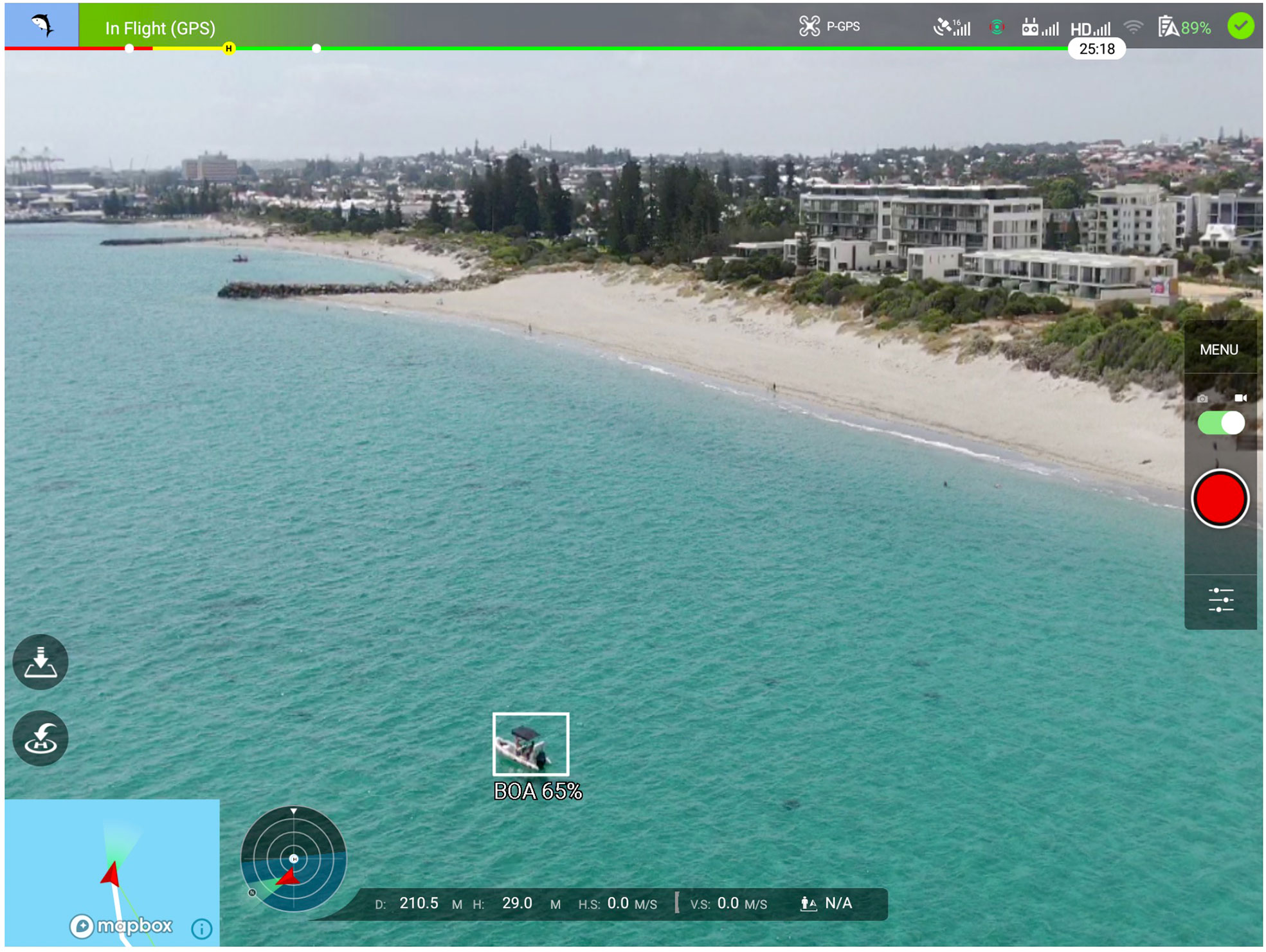
Figure 14 Screenshot of the mobile application flight screen as seen on a DJI CrystalSky Android tablet. The top bar includes information on (from left to right), flight status, GPS signal lock, GPS signal strength, telemetry signal strength, video signal strength, WiFi connectivity of tablet, drone battery status and controller connection status. The widget on the right hand side exposes camera settings and allows the user to record videos, or take a pictures, that are saved to the drone’s on-board storage. On the left hand side are controls to command the drone to land (upper button) and return to home (lower button). Along the bottom of the screen is information on drone location and movement. From left to right: map widget, compass/heading widget, distance from controller, height, horizontal speed and vertical speed. The deep learning model has identified a boat on the current frame and annotated it with a white box and label ‘BOA 65%’, indicating the confidence of the detection. Note that the location of the box and the boat do not coincide exactly due a short time lag between detecting the boat and drawing the box.

Beyond this standard interface, we augmented the video feed display with a new overlay showing the results of the object detector. Detected objects are annotated in real-time with rectangular bounding boxes, predicted labels and detection confidence scores (e.g., the white box shown in Figure 14).

6.1.1 App development and functionality

The app was developed in Android Studio¹⁰, employing the DJI Software Development Kit¹¹, V 4.15 to build the flight interface and the Tensorflow Lite¹² library (V 2.5) for performing object detection inference. The DJI SDK provides many pre-packaged flight widgets for Android and manages the connection to the drone and controller. However, apps that make use of the SDK must register with DJI servers via an internet connection the first time they are deployed after installation on a new device.

The object detection system was implemented to run in a background process that runs concurrently with the video decoding system. During operation, the detector grabs the latest available frame, pushes it though the neural network, applies non-maximum-suppression and confidence filtering to the results, and updates the detection box overlay shown to the user. Processing each frame takes of order ~ 500 ms on a CrystalSky CPU, meaning that the detection step is only run on one frame in 10 or 15. This is perceived by pilots as a slight lag in the boxes drawn on the screen compared to the location of a moving target - only an issue if the video scene is panning rapidly.

6.2 Model performance in the field

In order to assess the performance of the MobileNet model running on the CrystalSky tablet compared to a GPU-accelerated desktop, we captured the inference output in real time¹³. Each box that was drawn on the screen was also captured in a CSV file, with information on time, bounding box coordinates, predicted label and confidence recorded. Unfortunately, the time stamp saved was local to the CrystalSky, which in the field proved to be unreliable. This meant that it was not possible to use time-stamps to accurately co-register the app-based predictions with the equivalent desktop-based predictions (i.e., when the model was later applied to the recorded video by processing on a desktop computer). Instead, we treated the time stamps as an estimate and roughly aligned the two prediction time-series. We then directly compared the location of boxes within the video footage to find as close a match as possible, taking into account the inference lag (~ 0.5 s) introduced by our prototype code. Because of these difficulties in accurately matching outputs, we provide only qualitative results comparing the performance of the model in the field to a desktop implementation.

Overall, we found the outputs to be similar, with boxes reliably drawn over a target animal, together with the correct classification successfully achieved on most frames. However, we noticed that the mean confidence score was lower for the model run on the mobile device (67%), compared to the desktop (77%). We stress that these numbers should be compared as a guide only due to the differences in how candidate predictions were processed on the mobile device compared to the desktop computer. We also noted that both models had similar levels of false positive and false negative detections, which were greatly reduced after the introduction of ‘negative’ fields into the training data. This gives us confidence that the final MobileNet V1 model will be a useful tool in the field and the performance of desktop and mobile models can be brought to parity.

7 Discussion and future work

The results presented in §5 and §6 show that ML-driven object detection models can do an excellent job of distinguishing shark species - if they have been trained using an accurately-labelled, diverse and well-normalised dataset. Figures 8 and 10 illustrate the likely performance of moderate and small-sized neural networks (ResNet-50 and MobileNet V1, respectively) once they have been tuned to a location and season. However, the drop in performance on the external testing data (Figures 9 and 11) also shows that the current archive of video footage is far from ideal. The image ingest size and network architecture of both models impose fundamental limitations on the size of objects that can be reliably detected. The key lessons to be learned from this study are as follows:

From the perspective of the network, not all species are created equal. Neural network object detectors mimic human vision systems, so this is an obvious point. Just as expert observers sometimes struggle to distinguish between shark species, so do neural networks, and for the same reason: the differentiating features of similar species are obscured when data quality is poor. A good example of this is the confusion between whaler and white sharks when the turbidity or surface distortion is high, when the animals are deep in the water column, or simply appear small in the images. A detailed analysis of the factors affecting the performance of the neural networks is outside the scope of this work, however, we point to the comprehensive study by Dujon et al. (2021) as an example of how such analysis could be conducted. This would require a carefully designed data collection campaign that measures confounding variables such as water turbidity, sun glitter and animal depth.

The angular size of targeted objects is a limitation for all networks and architectures should be chosen appropriately. While the ResNet-50 and MobileNet V1 backbone architectures performed very well in this study, smaller objects are less reliably detected and labelled by both. This effect is greater for our implementation of MobileNet V1, leading to a steep drop-off in confidence for objects smaller than ~ 55 pixels. For best performance, objects should be greater than 80 pixels in size. For example, to guarantee a reliable identification a 2 m shark, a Mavic 2 Enterprise drone would need to be operating at an altitude of 25 m¹⁴. This effect was experienced first-hand during the trials of the prototype mobile application run by SLS NSW in early 2020. Based on this, we recommend that pilots can fly at a cruising altitude of 50 m, where we expect smaller objects to be detected, but not necessarily correctly classified (see Figure 12). Once an object has been detected and the pilot decides further investigation is warranted, the drone should drop to a height of 25 m for a reliable classification. A custom version of MobileNet V1 with a native 1080p ingest resolution would significantly improve the sensitivity to smaller objects, but we leave this for future work.

A diverse and well-normalised training dataset is crucial. The major limitation on detector reliability is imposed by the small sample size for certain object classes. This can also be a problem for classes with large numbers of boxes that are extracted from only a few videos, or from drone flights that sample a narrow range of environmental conditions. In these cases, the training data will not be representative of the full gamut of conditions encountered in the field. Managing and augmenting the distributions of training data properties is the most critical step in a supervised machine-learning workflow, with the largest impact on the real-world performance (see the movement for Data-Centric AI espoused by Andrew Ng - Ng, 2021). One promising approach to mitigating the class imbalance problem is to generate realistic synthetic data by using generative adversarial networks (GANs). In their review, Sampath et al. (2021) suggest that a blend of real and GAN-generated images have enormous potential to increase performance, especially if combined with autoencoders to perform feature-space manipulations.

A robust end-to-end data collection system is required to guarantee high quality data. Harvesting data during the 2020 drone trials was a very labour-intensive process. Videos were copied from high-capacity memory cards and manually tagged with meta-data (e.g., location and date), before being added to the data archive. Unfortunately, the contracted pilots recorded almost all videos at low resolution, despite the flight checklist and trial protocol specifying ‘4K resolution only’. In addition, the video data for an entire beach location was lost and presumed destroyed. Access to a significant tranche of high-resolution data would have allowed us to better correct the effects of distribution shifts between classes (e.g., the size biases in the white shark data seen in Figure 6).

The data preparation and model training pipeline must be optimised for fast turn-around times. The pipeline developed for this work is designed around running multiple experiments in a research workflow. Discounting the labelling process, the time required to prepare data and train a model is approximately five days. This is also a manually driven process, requiring a user to initiate tasks in a sequence. A production system needs to be fully automated and significantly faster: continually ingesting new data, training new models on a daily basis and providing instant access to reports of model performance and system health. The system should also allow multiple parallel workflows and offer a version control system for both datasets and models. Environmental conditions will drift over time, leading to a drop in system performance, so the challenge is to iteratively update models to track this drift. The deployment and management of ML-models is now recognised as an essential service known as ML operations, or ‘MLOps’. For excellent overviews see Sculley et al. (2015) and Paleyes et al. (2021).

7.1 Vision for the future

We believe that ML-driven shark species detectors will be excellent decision-support tools for beach managers in the very near future. The technology is already changing the way ecologists survey marine fauna (e.g., Butcher et al., 2021; Dujon et al., 2021; Jenrette et al., 2022; Marrable et al., 2022; Zhang et al., 2022; Shi et al., 2022). Humans will always need to be included in the decision loop, but the human role will change as the ML models become more reliable and flight systems become more automated. Initially, beach managers will be guided by the results of the ML model, but will be aware of how the model degrades in poor conditions and will fold this knowledge into their decision-making process. Over time, new data will sample unexplored parameter space and - if managed correctly - the system will learn to make better predictions, earning trust from experts and users alike.

Note that the system developed during this work represents a ‘no-frills’ baseline and there are a myriad of ways in which each component could be improved. For example:

● Pre-processing the video imagery to enhance salient features of sharks (see, for example, the image-enhancement algorithm of Sun et al., 2022).

● Using active learning loops while training, which force the network to concentrate on the most difficult misidentified examples.

● Introducing time-domain information, either before inference (e.g., by selecting the best frames in a time window), or during inference by using a time-aware network that can extract information over a series of frames (e.g., recurrent neural networks, or attention layers Shi et al., 2022).

● Making the algorithm aware of hierarchical labelling structures and taxonomic relationships (e.g., Zhu and Bain, 2017).

● Exploring a wider range of network architecture and optimizing the training hyperparameters.

● Automatically characterising the properties of new data when adding to the data archive and continuously creating balanced training datasets.

● Using generative ML algorithms to carefully create artificial data to fill sparsely sampled categories or environmental conditions (see Sampath et al., 2021).

It is also important to note that the system presented here makes predictions on a frame-by-frame basis and all of the results reflect this. When deploying the model at the beach, we recommend that the production version of the mobile application employ object tracking to average the predicted labels in time and filter for spurious detections. For example, a simple IoU-based tracker has been demonstrated by Bochinski et al. (2017; 2018) to work extremely well for CNN-based object detectors with high frame rates. Presenting the user with the most common label in a short time window will mean that an occasional incorrectly predicted label will not be visible. An experienced user will also be capable of assessing detection quality and will naturally give more weight to labels generated when the conditions are better. For example, a blurry white shark deep under the surface may be labeled as a ‘whaler shark’ initially, but the label may change to ‘white shark’ as the animal approaches the surface and its true shape becomes apparent.

7.1.1 Towards full automation

Reliably automating the detection and identification of marine objects not only offers the potential to alleviate some of the human error in shark-spotting (Brack et al., 2018), but creates opportunity to use more advanced drone platforms that can run surveillance autonomously, and alert beach authorities when a potentially dangerous shark is detected. Recent technological developments have allowed such autonomous drone platforms to be developed (i.e., drones that can operate beyond line-of-sight from a drone enclosure without human intervention). Aviation restrictions and associated costs with beyond line-of-sight operations have typically limited the use case in ecological applications (Colefax et al., 2017; Angliss et al., 2018), however, regulations are adapting to accommodate drone autonomy (Merkert and Bushell, 2020). This rapidly evolving space is anticipated to usher in a paradigm change in how marine ecology is performed, delivering an automated near-real-time census of marine faunal populations (see also the review by Butcher et al., 2021).

8 Summary

In summary, we have systematically investigated the ability of modern machine learning algorithms to correctly detect and identify species of sharks and other fauna in aerial imagery from drones. We built a research software pipeline to facilitate the creation of labelled data, train instances of machine-learning models and analyse their performance. We also deployed a quantised model to an Android OS mobile device in a prototype application that performed inference on a live video feed. Our key results in this work are:

1. The RetinaNet object detection model, using both ResNet-50 and MobileNet V1 backbone architectures, displays excellent performance (mAP ≈ 95%) at distinguishing between shark species when tested on an internal testing dataset. In ideal conditions, and with appropriate training data, these model architectures will be highly reliable for finding and tracking marine fauna and other objects.

2. Tests performed on challenging external data give a better indication of true performance in the field. We find that the mean average precision of the MobileNet V1 model falls to mAP ≈ 60%, however, dangerous sharks are correctly detected 80% of the time. The drop in performance suggests that the models need to be carefully ‘tuned’ to new beach locations and environmental conditions.

3. Most of the performance issues identified via testing on the external data can be traced back to biases, imbalances or distribution shifts in the training data. We identify the correction of these issues as the best way to improve model performance in the future. The current labelled data, drawn mostly from the NSW DPI Phase 3 and 4 Drone Trials, are not ideal for training a highly-accurate shark species classifier. New high-resolution data should be gathered to sample rare classes, new beaches and a wider range of conditions. Alternatively, useful artificial data could be created using generative ML methods.

4. The false-positive rate is low for both models. During development we found that robust sampling of a dedicated ‘negative’ class was essential to achieving this result. This also means that both models will function well to locate objects of interests, even if the predicted labels are sometimes incorrect.

5. The reliability of detections dropped rapidly below a characteristic object size for both models (~ 55 pixels for our implementation of MobileNet V1). This is an intrinsic property of each network architecture combined with the ingest image size of the network. We recommend that pilots fly at a cruising altitude of 50 m to initially detect marine fauna, but then drop to a height of 25 m to secure a reliable classification.

6. The performance of a mobile application running real-time inference on a live video feed is good enough to act as a useful decision-support tool for beach managers and ecologists.

We have shown here that ML-enabled tools offer significant benefits when carefully deployed as part of a shark management strategy. Our results show that they can attain high accuracies, leading to greater reliability of shark-spotting from drones and have the potential to automate the monitoring coastal health. However, creating a trustworthy ML-enhanced shark-spotting system hinges on gathering (or generating) a balanced dataset, and likely requires an integrated MLOps pipeline for continuous model tracking and tuning.

Data availability statement

Raw data from the NSW DPI Drone Trials is property of the NSW Department of Primary Industries and access requests should be directed to the NSW DPI Fisheries Division. Further data will be made available at https://github.com/crpurcell/SharkAI at the authors’ discretion.

Author contributions

CP and AW developed the deep learning models and training pipeline for this publication. AW and AC performed the expert identification of marine fauna, and developed the labelled dataset used to train the models. PB provided expert evaluation of the final labelled data and project management for the live trials. All authors contributed to the drafting of the manuscript, including writing up results and discussion, and creating figures. All authors contributed to the article and approved the submitted version.

Funding

CP and AW were supported by a Macquarie University New Staff Grant. Drone footage was collected under NSW DPI and Office of Environment and Heritage scientific permits (Ref. P01/0059; MWL000102746) and animal ethics (16/09 – SIMS). Project funding and support was provided by NSW DPI and associated NSW Shark Management Strategy, and NSW DPI and Macquarie University grant: ‘Improved drone detection using artificial intelligence and portable devices’, CONT19/673 for CRP, AW and PB.

Acknowledgments

This work was also supported by Fujitsu Australia PTY LTD, who generously loaned a server containing a NVIDIA Tesla V100 GPU for training models. In particular, the support of Fujitsu employee Joel Lopez was instrumental to the project. The authors would like to thank the staff of Surf Life Saving NSW, who battled adversity to collect high-quality footage. The authors are also very grateful to Robert Gorkin III who kindly provided access to data for rare species, leading to a more comprehensive external testing dataset. We are indebted to NSW DPI Shark Programs Lead Marcel Green for comments that greatly improved the quality of this paper.

Conflict of interest

Authors AW and AC were employed by Sci-eye PTY LTD during the final stage of this project. CP was also a co-founder of Sci-eye PTY LTD but ceased employment in early 2022. CP currently works for Trillium Technologies PTY LTD and is an Adjunct Senior Lecturer at UNSW. The bulk of the research presented here was conducted prior to June 2020 in a purely academic setting and finalised during 2021 and 2022. PB declares that the research was conducted in the absence of any commercial or financial relationships that could be construed as a potential conflict of interest.

Publisher’s note

All claims expressed in this article are solely those of the authors and do not necessarily represent those of their affiliated organizations, or those of the publisher, the editors and the reviewers. Any product that may be evaluated in this article, or claim that may be made by its manufacturer, is not guaranteed or endorsed by the publisher.

Footnotes

1. ^ https://www.afid.io/.
2. ^ https://therippergroup.com.
3. ^ https://github.com/fizyr/keras-retinanet.
4. ^ https://github.com/tensorflow/models/tree/master/research/object.
5. ^ https://github.com/rafaelpadilla/Object-Detection-Metrics.
6. ^ https://www.dji.com/au/crystalsky.
7. ^ https://www.dji.com/au/smart-controller.
8. ^ https://www.dji.com/au/mavic-2-enterprise.
9. ^ https://store.dji.com/guides/dji-go-4-manual/.
10. ^ https://developer.android.com/studio.
11. ^ https://developer.dji.com/mobile-sdk/.
12. ^ https://www.tensorflow.org/lite.
13. ^ Due to time and technical limitations, the version of Mobilenet V1 deployed to the prototype Android application was a ‘reduced width’ model, with α = 0.75.

References

Angliss R. P., Ferguson M. C., Hall P., Helker V., Kennedy A., Sformo T. (2018). Comparing manned to unmanned aerial surveys for cetacean monitoring in the arctic: methods and operational results. J. Unmanned. Vehicle. Syst. 6, 109–127. doi: 10.1139/juvs-2018-0001

CrossRef Full Text | Google Scholar

Bochinski E., Eiselein V., Sikora T. (2017). “High-speed tracking-by-detection without using image information,” Proc. IEEE 14th Int. Conf. Adv. Video Signal Based Surveill (Lecce, Italy: IEEE), 1–6.

Google Scholar

Bochinski E., Senst T., Sikora T. (2018). “Extending iou based multi-object tracking by visual information,” in IEEE International conference on advanced video and signals-based surveillance (Auckland, New Zealand), 441–446.

Google Scholar

Box G. E. P., Cox D. R. (1964). An analysis of transformations. J. R. Stat. Soc. 26, 211–252. doi: 10.1111/j.2517-6161.1964.tb00553.x

CrossRef Full Text | Google Scholar

Brack I. V., Kinde l A., Oliveira L. F. B., Scales K. (2018). Detection errors in wildlife abundance estimates from unmanned aerial systems (uas) surveys: Synthesis, solutions, and challenges. Methods Ecol. Evol. 9, 1864–1873. doi: 10.1111/2041-210x.13026

CrossRef Full Text | Google Scholar

Burke C., Rashman M. F., Longmore S. N., McAree O., Glover-Kapfer P., Ancrenaz M., et al. (2019). Successful observation of orangutans in the wild with thermal-equipped drones. J. Unmanned. Vehicle. Syst. 7, 235–257. doi: 10.1139/juvs-2018-0035

CrossRef Full Text | Google Scholar

Burr P., Samiappan S., Hathcock L., Moorhead R., Dorr B. (2019). Estimating waterbird abundance on catfish aquaculture ponds using an unmanned aerial system. Human-Wildlife. Interact. 1–13. doi: 10.26077/ahd5-na26

CrossRef Full Text | Google Scholar

Butcher P. A., Colefax A. P., Gorkin R. A., Kajiura S. M., López N. A., Mourier J., et al. (2021). The drone revolution of shark science: A review. Drones 5, 8. doi: 10.3390/drones5010008

CrossRef Full Text | Google Scholar

Butcher P., Piddock T., Colefax A., Hoade B., Peddemors V., Borg L., et al. (2019). Beach safety: Can drones provide a platform for sighting sharks? Wildlife Res 46, 701–712. doi: 10.1071/wr18119

CrossRef Full Text | Google Scholar

Byles K. (2016). “Automated shark detection using computer vision. master’s thesis,” in ENG4112 honours research project (University of Southern Queensland, Faculty of Health, Engineering & Sciences). Available at: https://eprints.usq.edu.au/31382/. Last accessed Oct 2022.

Google Scholar

Chabot D. (2018). Trends in drone research and applications as the journal of unmanned vehicle systems turns five. J. Unmanned. Vehicle. Syst. 6, vi–xv. doi: 10.1139/juvs-2018-0005

CrossRef Full Text | Google Scholar

Chapman A. (2014). It’s okay to call them drones. J. Unmanned. Vehicle. Syst. 02, iii–iiv. doi: 10.1139/juvs-2014-0009

CrossRef Full Text | Google Scholar

Chen X., Tung Y.-K. (2003). Investigation of polynomial normal transform. Struct. Saf. 25, 423–445. doi: 10.1016/S0167-4730(03)00019-5

CrossRef Full Text | Google Scholar

Colefax A. P., Butcher P. A., Kelaher B. P. (2017). The potential for unmanned aerial vehicles (UAVs) to conduct marine fauna surveys in place of manned aircraft. ICES. J. Mar. Sci. 75, 1–8. doi: 10.1093/icesjms/fsx100

CrossRef Full Text | Google Scholar

Colefax A. P., Butcher P. A., Pagendam D. E., Kelaher B. P. (2019). Reliability of marine faunal detections in drone-based monitoring. Ocean. Coast. Manage. 174, 108–115. doi: 10.1016/j.ocecoaman.2019.03.008

CrossRef Full Text | Google Scholar

Colefax A. P., Butcher P. A., Pagendam D. E., Kelaher B. P. (2020b). Comparing distributions of white, bull, and tiger sharks near and away from the surf break using three tech-based methods. Ocean. Coast. Manage. 198, 105366. doi: 10.1016/j.ocecoaman.2020.105366

CrossRef Full Text | Google Scholar

Colefax A. P., Kelaher B. P., Pagendam D. E., Butcher P. A. (2020a). Assessing white shark (carcharodon carcharias) behavior along coastal beaches for conservation-focused shark mitigation. Front. Mar. Sci. 7. doi: 10.3389/fmars.2020.00268

CrossRef Full Text | Google Scholar

Draper J. (1952). Properties of distributions resulting from certain simple transformations of the normal distribution. Biometrika 39, 290–301. doi: 10.2307/2334025

CrossRef Full Text | Google Scholar

Dujon A. M., Ierodiaconou D., Geeson J. J., Arnould J. P. Y., Allan B. M., Katselidis K. A., et al. (2021). Machine learning to detect marine animals in uav imagery: effect of morphology, spacing, behaviour and habitat. Remote Sens. Ecol. Conserv. 7, 341–354. doi: 10.1002/rse2.205

CrossRef Full Text | Google Scholar

Eikelboom J., Wind J., Ven E., Kenana M., Schroder B., Knegt H., et al. (2019). Improving the precision and accuracy of animal population estimates with aerial image object detection. Methods Ecol. Evol 10, 1–13. doi: 10.1111/2041-210X.13277

CrossRef Full Text | Google Scholar

Gasser T., Bächer P., Möcks J. (1982). Transformations towards the normal distribution of broad band spectral parameters of the eeg. Electroencephalogr. Clin. Neurophysiol. 53, 119–124. doi: 10.1016/0013-4694(82)90112-2

PubMed Abstract | CrossRef Full Text | Google Scholar

Gorkin R., Adams K., Berryman M. J., Aubin S., Li W., Davis A. R., et al. (2020). Sharkeye: Real-time autonomous personal shark alerting via aerial surveillance. Drones 4, 18. doi: 10.3390/drones4020018

CrossRef Full Text | Google Scholar

Hodgson J., Mott R., Baylis S., Pham T., Wotherspoon S., Kilpatrick A., et al. (2018). Drones count wildlife more accurately and precisely than humans. Methods Ecol. Evol 9, 1160–1167. doi: 10.1111/2041-210X.12974

CrossRef Full Text | Google Scholar

Jenrette J., Liu Z. Y.-C., Chimote P., Hastie T., Fox E., Ferretti F. (2022). Shark detection and classification with machine learning. Ecol. Inf. 69, 101673. doi: 10.1016/j.ecoinf.2022.101673

CrossRef Full Text | Google Scholar

Li X., Huang H., Savkin A. V. (2020). “Autonomous drone shark shield: a novel shark repelling system for protecting swimmers and surfers,” in 6th Internationsl Conference on Control, Automation, and Robotics (ICCAR). 455–458. doi: 10.1109/ICCAR49639.2020.9107984

CrossRef Full Text | Google Scholar

Lin T.-Y., Goyal P., Girshick R., He K., Dollár P. (2017). Focal loss for dense object detection. IEEE Trans. Pattern Anal. Mach. Intell. 42, 318–327. doi: 10.1109/TPAMI.2018.2858826

CrossRef Full Text | Google Scholar

Liordos V., Kontsiotis V. J., Georgari M., Baltzi K., Baltzi I. (2017). Public acceptance of management methods under different human-wildlife conflict scenarios. Sci. Total. Environ. 579, 685–693. doi: 10.1016/j.scitotenv.2016.11.040

PubMed Abstract | CrossRef Full Text | Google Scholar

Longmore S. N., Collins R. P., Pfeifer S., Fox S. E., Mulero-Pazmany M., Bezombes F., et al. (2017). Adapting astronomical source detection software to help detect animals in thermal images obtained by unmanned aerial systems. Int. J. Remote Sens. 38, 2623–2638. doi: 10.1080/01431161.2017.1280639

CrossRef Full Text | Google Scholar

Maire F., Mejias L., Hodgson A. (2014). “A convolutional neural network for automatic analysis of aerial imagery,” in Digital image computing: Techniques and applications (DICTA 2014). Eds. Wang L. W., Ogunbona P., Li W. (New South Wales, Australia: Wollongong).

Google Scholar

Maire F., Mejias L., Hodgson G, A., Duclos G. (2013). “Detection of dugongs from unmanned aerial vehicles,” IEEE International Workshop on Intelligent Robots and Systems(IROS), 2750–2756. doi: 10.1109/ICCAR49639.2020.9107984

CrossRef Full Text | Google Scholar

Marrable D., Barker K., Tippaya S., Wyatt M., Bainbridge S., Stowar M., et al. (2022). Accelerating species recognition and labelling of fish from underwater video with machine-assisted deep learning. Front. Mar. Sci. 9. doi: 10.3389/fmars.2022.944582

PubMed Abstract | CrossRef Full Text | Google Scholar

Mazumder M., Banbury C., Yao X., Karlaš B., Gaviria Rojas W., Diamos S., et al. (2022). DataPerf: Benchmarks for data-centric AI development. arXiv 2207.10062. doi: 10.48550/arXiv.2207.10062

CrossRef Full Text | Google Scholar

McPhee D. P., Blount C. (2015). Shark deterrents and detectors:. Review of bather protection technologies (Cardno, St Leonards, NSW: NSW Department of Primary Industries).

Google Scholar

Merkert R., Bushell J. (2020). Managing the drone revolution: A systematic literature review into the current use of airborne drones and future strategic directions for their effective control. J. Air. Transp. Manag. 89, 101929. doi: 10.1016/j.jairtraman.2020.101929

PubMed Abstract | CrossRef Full Text | Google Scholar

Ng A. (2021) Data-centric AI competition. Available at: https://https-deeplearning-ai.github.io/data-centric-comp/ (Accessed 15-May-2022).

Google Scholar

Padilla R., Passos W. L., Dias T. L. B., Netto S. L., da Silva E. A. B. (2021). A comparative analysis of object detection metrics with a companion open-source toolkit. Electronics 10, 297. doi: 10.3390/electronics10030279

CrossRef Full Text | Google Scholar

Paleyes A., Urma R.-G., Lawrence N. D. (2021). Challenges in deploying machine learning: a survey of case studies. arXiv 2011. 09926. doi: 10.1145/3533378

CrossRef Full Text | Google Scholar

Pepin-Neff C., Wynter T. (2018a). Shark bites and shark conservation: An analysis of human attitudes following shark bite incidents in two locations in australia. Conserv. Lett. 11, e12407. doi: 10.1111/conl.12407

CrossRef Full Text | Google Scholar

Pepin-Neff C. L., Wynter T. (2018b). Reducing fear to influence policy preferences: An experiment with sharks and beach safety policy options. Mar. Policy 88, 222–229. doi: 10.1016/j.marpol.2017.11.023

CrossRef Full Text | Google Scholar

Pyrrö P., Naseri H., Jung A. (2021). AIR: Aerial inspection RetinaNet for land search and rescue missions (Aalto University, School of Science) Avail:https://aaltodoc.aalto.fi/handle/123456789/112856. Last accessed Oct 2022.

Google Scholar

Raoult V., Colefax A. P., Allan B. M., Cagnazzi D., Castelblanco-Martínez N., Ierodiaconou D., et al. (2020). Operational protocols for the use of drones in marine animal research. Drones 4, 64. doi: 10.3390/drones4040064

CrossRef Full Text | Google Scholar

Roberts M., Driggs D., Thorpe M., Gilbey J., Yeung M., Ursprung S., et al. (2021). Common pitfalls and recommendations for using machine learning to detect and prognosticate for covid-19 using chest radiographs and ct scans. Nat. Mach. Intell. 3, 199–217. doi: 10.1038/s42256-021-00307-0

CrossRef Full Text | Google Scholar

Sampath V., Maurtua I., Aguilar Martín J. J., Gutierrez A. (2021). A survey on generative adversarial networks for imbalance problems in computer vision tasks. J. Big. Data 8, 27. doi: 10.1186/s40537-021-00414-0

PubMed Abstract | CrossRef Full Text | Google Scholar

Sculley D., Holt G., Golovin D., Davydov E., Phillips T., Ebner D., et al. (2015). “Hidden technical debt in machine learning systems,” in Proceedings of the 28th international conference on neural information processing systems, vol 28. MIT Press.

Google Scholar

Sharma N., Saqib M., Scully-Power P., Blumenstein M. (2022). SharkSpotter: Shark detection with drones for human safety and environmental protection (Cham: Springer International Publishing), 223–237. doi: 10.1007/978-3-030-72188-6_11

CrossRef Full Text | Google Scholar

Sharma N., Scully-Power P., Blumenstein M. (2018). “Shark detection from aerial imagery using region-based cnn, a study,” in AI 2018: Advances in artificial intelligence. Eds. Mitrovic T., Xue B., Li X. (Cham: Springer International Publishing), 224–236.

Google Scholar

Shi Z., Guan C., Li Q., Liang J., Cao L., Zheng H., et al. (2022). Detecting marine organisms via joint attention-relation learning for marine video surveillance. IEEE J. Oceanic. Eng. (early access), 1–16. doi: 10.1109/JOE.2022.3162864

CrossRef Full Text | Google Scholar

Simmons P., Mehmet M. I. (2018). Shark management strategy policy considerations: Community preferences, reasoning and speculations. Mar. Policy 96, 111–119. doi: 10.1016/j.marpol.2018.08.010

CrossRef Full Text | Google Scholar

Stokes D., Apps K., Butcher P. A., Weiler B., Luke H., Colefax A. P. (2020). Beach-user perceptions and attitudes towards drone surveillance as a shark-bite mitigation tool. Mar. Policy 120, 104127. doi: 10.1016/j.marpol.2020.104127

CrossRef Full Text | Google Scholar

Sun S., Wang H., Zhang H., Li M., Xiang M., Luo C., et al. (2022). Underwater image enhancement with reinforcement learning. IEEE J. Oceanic. Eng. (early access), 1–13. doi: 10.1109/JOE.2022.3152519

CrossRef Full Text | Google Scholar

Taylor J., McLean L., Korner A., Glozier N. (2019). Direct and indirect psychological impacts of shark-bite events. Aust. N. Z. J. Psychiatry 53, 27–36. doi: 10.1177/0004867418808899

PubMed Abstract | CrossRef Full Text | Google Scholar

van Albada S. J., Robinson P. A. (2018). Transformation of arbitrary distributions to the car. arXiv 1801.01748. doi: 10.48550/arXiv.1801.01748

CrossRef Full Text | Google Scholar

Zhang J., Wang S., Zhang S., Tang F., Fan W., Yang S., et al. (2022). Research on target detection of engraulis japonicus purse seine based on improved model of yolov5. Front. Mar. Sci. 9. doi: 10.3389/fmars.2022.933735

PubMed Abstract | CrossRef Full Text | Google Scholar

Zhou H., Llewellyn L., Wei L., Creighton D., Nahavandi S. (2015). “Marine object detection using background modelling and blob analysis,” in IEEE International Conference on Systems, Man, and Cybernetics. 430–435. doi: 10.1109/SMC.2015.86

CrossRef Full Text | Google Scholar

Zhu X., Bain M. (2017). B-CNN: Branch convolutional neural network for hierarchical classification. arXiv 1709.09890. doi: 10.48550/arXiv.1709.09890

CrossRef Full Text | Google Scholar