Abrupt chlorophyll shift driven by phosphorus threshold in a small subtropical estuary

Introduction

Abrupt ecological shifts in trophic structure, community structure, and organism abundance are reported across all marine ecosystems (Daskalov, 2002; Charpentier et al., 2005; Cloern et al., 2007; Cloern et al., 2010; Auber et al., 2015). Abrupt shifts can occur for ecosystem states, defined as quantitative descriptions of multiple attributes of a system, or for ecological responses (Mac Nally et al., 2014). Ecological responses include measures of organism biomass, species abundance, or primary production (Mac Nally et al., 2014). While definitions of abrupt shifts vary, a credible abrupt shift should demonstrate a meaningful difference in ecosystem state or ecological response before and after the shift and be supported with evidence of a pressure that caused the shift (Lees et al., 2006; Capon et al., 2015). The pressures that cause abrupt shifts, as well as the shifts themselves, are varied across the marine literature. In San Francisco Bay, a change in the California Current System caused a trophic cascade that resulted in increased phytoplankton biomass (Cloern et al., 2007). In the Hudson River Estuary, the introduction of zebra mussels resulted in a regime shift in the littoral food web and a decrease in phytoplankton biomass (Strayer et al., 2008). Other pressures such as climate, salinity, and nutrients have been demonstrated to cause shifts relating to phytoplankton, seagrasses, and sediment macrofauna, respectively (Lehman, 2000; Charpentier et al., 2005; Hewitt and Thrush, 2010).

While abrupt shifts are commonly reported in marine literature, they do not all fulfill the criteria of a sudden change. In a review of estuarine and nearshore systems, Mac Nally et al. (2014) found that only eight papers out of the 98 reviewed demonstrated a “stark ecological change” that was credibly linked to a pressure change. Many reported shifts were inferred from spatial, rather than temporal, changes and evidence was often derived from just two points in time instead of from a time series (Mac Nally et al., 2014). Long-term time series play a critical role in detecting ecological shifts; without them, shifts cannot be discerned from the various other changes that occur over numerous time scales. Decadal time series are required for determination of the frequency and duration of changes, thus allowing categorization of variability that could be periodic, monotonic, or abrupt (Cloern, 2019).

This study utilized an 18-year chlorophyll-a (chl-a) time series from Weeks Bay, a small, subtropical estuary in southern Alabama, to understand patterns of chlorophyll variability over multiple time scales and to investigate mechanisms of this variability. Weeks Bay is part of the National Oceanic and Atmospheric Administration (NOAA)’s National Estuarine Research Reserve System (NERRS). The NERRS consists of 30 estuaries across the United States and is a network designed to protect and study these transition zones; as such, a system-wide monitoring program (SWMP) is in place at all the NERRS estuaries. The lengthy 18-year chl-a time series from Weeks Bay’s SWMP offered a unique opportunity to identify trends in chl-a that occur over various time scales, reflecting the seasonal, annual, interannual, or event-based nature of the processes that drive variability (Cloern and Jassby, 2010). Measures of environmental variables can pinpoint trends or changes in these processes, whether they be nutrient fluctuations caused by human disturbances or modifications in freshwater flow governed by hydrology and climate. We supplemented the chl-a time series with up to 30 years of time series data for nutrients (nitrogen and phosphorus), hydrology (river discharge and salinity), and climate (temperature) to better understand the processes of these variables and their relationships with chlorophyll.

Trends in chlorophyll variability are still uncharacterized in many marine systems, despite extensive advances in eutrophication science over the past several decades (Smith and Schindler, 2009; Carstensen et al., 2015). Tropical and subtropical estuaries are especially under-sampled and may reveal new patterns that add to knowledge learned from temperate estuaries (Carstensen et al., 2015). The SWMP data set used herein is also available at the 29 other NERRS sites, some of which are in subtropical or tropical regions. To our knowledge, these SWMP data have only been utilized in publication once before by Baumann and Smith (2017). Baumann and Smith (2017) compiled and analyzed 15 years of pH and dissolved oxygen (DO) SWMP data from 16 NERRS sites. Despite the considerable geomorphic differences between sites, Baumann and Smith (2017) derived strong empirical relationships between pH and DO across all sites, indicating that variability in DO could be used to predict pH conditions across most coastal systems. Following Baumann and Smith’s example, the analyses conducted herein could be applied all NERRS sites with sufficient length of data sets (determined by their date of NERR designation) and would result in a more complete geographic understanding of chlorophyll trends across United States coastal systems.

In Weeks Bay, chl-a concentrations are known to be high and eutrophication is a well-documented issue (Lehrter, 2008; Mortazavi et al., 2012). Nitrogen and phosphorus enrichment originates from residential/commercial and agricultural non-point sources as well as some municipal and industrial facility point sources (Lehrter, 2006; Tetra Tech Inc., 2013). The Weeks Bay watershed is dominated by agricultural land use but has experienced an increase in developed land use over the last couple decades. According to an analysis of a United States Geological Survey (USGS) National Land Cover Database (NLCD) data set, percent agricultural land use in the watershed decreased from 59% to 49% from 1992 to 2011 and was accompanied by an increase in developed land use from 2% to 13% that was driven by population growth (Thompson Engineering, 2017). Nitrogen and phosphorus concentrations entering Weeks Bay exhibited an overall increasing trend during this period (ADEM, 2014).

The expression of estuarine eutrophication due to nutrient loading is expected to be influenced by hydrology and climate, though the magnitude of effects and interactions between them are not well characterized. In small systems like Weeks Bay that have short water residence times (Lehrter, 2008), nutrient loads may be a poor indicator of eutrophication because the system may flush too quickly for phytoplankton blooms to form (Pennock and Sharp, 1986; Borsuk et al., 2004; Lehrter, 2008; Canion et al., 2013; Novoveska and MacIntyre, 2019). Thus, eutrophication in small shallow systems like Weeks Bay may be caused by high nutrient loads, but variability in phytoplankton biomass is also highly regulated by climate, physical mixing, and flushing time scales of the system.

Given the trend of increasing nutrients, we hypothesized that chl-a would exhibit a matching long-term increase that would be modulated by a positive relationship with temperature and a negative relationship with river discharge. We found that chl-a increased at three of the SWMP stations, and that this increase constituted a statistically significant abrupt shift in ecological response at two stations. The pattern of the chl-a trend at these two stations was different than that of phosphorus concentration (i.e., the limiting nutrient as demonstrated below) from the primary river system. Phosphorus concentration also exhibited an abrupt increase, but had a consistent increasing trend over the entire time series. We attributed the abrupt shift in chl-a concentration to the combined effect of a rarely described estuarine phosphorus threshold and very low river discharge rates and variability.

Methods

Study site

Weeks Bay is a small (7 km²), shallow (mean depth = 1.3 m) sub-estuary located off the southeastern portion of Mobile Bay (Miller-Way et al., 1996). The 18-year chl-a time series utilized in this study was a part of the SWMP at the Weeks Bay reserve and included measures of nutrient concentrations and other water quality parameters, described below.

SWMP monitoring at Weeks Bay occurred at four stations within the estuary. Data from the four SWMP stations and from a United States Geological Survey (USGS) gauge (USGS 02378500) on the Fish River near Silver Hill, AL, were used in this analysis (Figure 1). The Fish River provides 73% of the freshwater input to Weeks Bay, which has an overall watershed area of 526 km² (Thompson Engineering, 2017). Hereafter, variables from the Weeks Bay SWMP stations will be referred to as ‘SWMP’ in contrast to variables from the Fish River gauge that will be referred to as ‘gauge’.

FIGURE 1

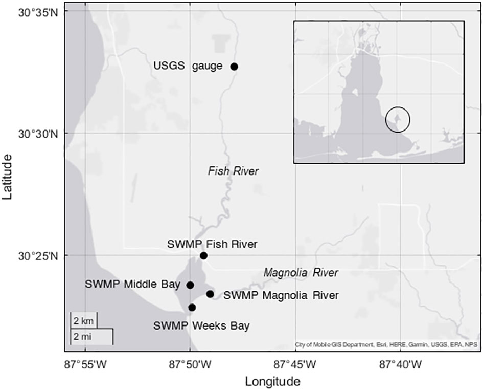
Figure 1 Site map of the Weeks Bay estuary. The USGS gauge is located upstream on the Fish River. The four SWMP stations were the Fish River (mean water depth = 2m), Magnolia River (1.1 m), Middle Bay (1.5 m), and Weeks Bay (0.9 m) stations. The Weeks Bay estuary is circled on the inset map of Mobile Bay, AL.

Data sets and compilation

Data for the SWMP stations in Weeks Bay were downloaded from the Centralized Data Management Office of the NERRS¹. Nutrient data for the gauge were downloaded from the Water Quality Portal² and Fish River discharge data were downloaded from the USGS³.

Chl-a concentrations from the SWMP stations were used as a proxy for phytoplankton biomass with the understanding that while cellular levels of chl-a vary with factors such as species type, irradiance, and physiological state of cells (Geider et al., 1997; Breton et al., 2000; Boyer et al., 2009), chl-a is typically strongly correlated to primary production (Cole and Cloern, 1987) and is the most common phytoplankton biomass measure available from monitoring programs (Cloern and Jassby, 2010). The other SWMP time series variables analyzed were temperature, salinity, and dissolved nutrients. These nutrients were ammonium (NH₄⁺), nitrite+nitrate (hereafter: NO₃^-), and phosphate (PO₄^3-). Monthly chl-a and nutrient data were available from 2002 to 2020 for all four stations. SWMP chl-a and nutrient measures were obtained from monthly surficial grab samples taken one hour prior to slack low tide. When possible, samples were collected under spring tide conditions. Chl-a was measured by EPA Method 445.0 and nutrients were measured with protocols described in Standard Methods for Examination of Water and Wastewater (APHA, 1998). Values for measures outside the low sensor range were logged as the method detection limit (MDL).

Due to missing data or data flagged as suspect by quality analysis procedures, photosynthetically active radiation (PAR) and turbidity data in the SWMP dataset were not considered in this analysis. Temperature and salinity time series were measured by hydrographic sondes (YSI EXO2) from 1995 to 2022 at the SWMP Fish River and Weeks Bay stations and from 2003 to 2022 at the SWMP Magnolia River and Middle Bay stations. Salinity and temperature were logged at 30-minute intervals until 2007. Thereafter, the data were logged at 15-minute intervals.

Chl-a, salinity, and temperature data were not available from the gauge. Time series data from the gauge included hourly river discharge and approximately monthly nutrient concentrations of dissolved NH₄⁺, NO₃^-, PO₄^3-, and total phosphorus (TP). However, there were some gaps in the nutrient data. Gauge nutrient concentrations reported as 0 mg l^-1 were below the MDL. Two other variables were calculated from the discharge data to describe modes of variability, i.e., baseflow index and flashiness (see below). River discharge at the gauge was available from 1994 to 2022. The data periods for gauge nutrients ranged from 1992 to 2020 for NH₄⁺, 1990 to 2020 for NO₃^-, 1990 to 2020 for TP, and 2005 to 2020 for PO₄^3-.

The methods for nutrient analysis at the gauge were largely consistent, though there were periods of unspecified method procedures for older data. TP analysis was conducted using EPA Method 365.1 from 2008 onwards. The majority of TP analyses before 2008 were also conducted using EPA Method 365.1, though a portion of these analyses were made using EPA Method 365.4 (F. Leslie, personal communication, August 11, 2022). The small proportion of measures made with EPA Method 365.4 were not expected to affect TP trends. Though earlier work suggested a difference of approximately 30% between EPA Methods 365.4 and 365.1 (Patton and Truitt, 1992), a more recent study indicated that the two methods were comparable and exhibited high correlation (r = 0.98) for concentrations ranging from 0 to 0.6 mg l^-1 (Chen et al., 2006). Other gauge nutrients, dissolved NH₄⁺, NO₃^-, and PO₄^3-, were analyzed by EPA Methods 350.1, 353.2, and 365.1, respectively, from the late 2000s to 2020. Prior to the late 2000s, the methods for these analytes were marked as “ADEM Historical” and were unknown. Any changes in methods for the analysis of NH₄⁺, NO₃^-, and PO₄^3- should not impact trend detection. Unlike TP, measurement of these nutrients does not require a chemical and/or high temperature extraction step from particulate or dissolved organic matter. The potential for differences between extraction efficiencies is the main concern when comparing TP concentrations measured using more than one method. For dissolved inorganic nutrient species, calibration with standard solutions is included in analysis and thus produces comparable results across methods for NH₄⁺, NO₃^-, and PO₄^3-.

Calculated variables

A monthly baseflow index (BFI) was calculated to assess the proportion of river discharge attributed to baseflow groundwater versus surface runoff (Gustard et al., 1992). Briefly, daily baseflow was determined from a rolling window of minimum daily discharge values in which center window values were identified as baseflow ordinates if they were less than 0.9 times outer window values. Baseflow values were then interpolated between baseflow ordinates. The volume beneath the baseflow line divided by the volume beneath the discharge line resulted in the baseflow index.

The Richards-Baker Flashiness Index (RBI) was calculated (Equation 1) to quantify the frequency and magnitude of river discharge extreme events according to the methods of Baker et al. (2004)

$$RBI= \frac{{\sum }_{i=1}^n\left|q_i-q_{i-1}\right|}{{\sum }_{i=1}^n{q}_i}$$

(1)

where the sum of the absolute value of the difference in daily discharge volume or flow (q_i) over a unit time was divided by the sum of the daily discharge volumes or flows over the same period. Flashiness is sensitive to the frequency and magnitude of storms events (Baker et al., 2004) and provides measures of these events that may be lost in mean river discharge values. The frequency and magnitude of changes in river discharge was especially relevant in our system, where flushing events were expected to have a considerable impact on chlorophyll dynamics. We calculated the RBI using a period length of one month.

Trend analysis

Following a procedure outlined by Cloern (2019), various statistical tests were performed to assess trends operating at different time scales. For visual inspection of trends, time series data were fit to a robust loess (rloess) curve with a 5-year window. To quantify temporal variability, time series were decomposed into annual, seasonal, and residual components using a multiplicative seasonal model (Equation 2) (Cloern and Jassby, 2010)

$$c_{ij}=C{y}_i{m}_j{\epsilon }_{ji}$$

(2)

where c_ij was the variable concentration in year i (i = 1,…,n) and month j (j=1,…,12), C was the long-term mean of the series, y_i was the annual component in the ith year, m_j was the seasonal component in the jth month, and ε_ij was the residual component. The annual component was calculated by dividing the annual mean by the overall series mean (y_i = Y_i/C), with values > 1 indicating years of above average conditions and values < 1 indicating years of below average conditions. The seasonal component was calculated by dividing the variable for month j in year i by the annual mean (m_ij = M_ij/Y_i), with values > 1 indicating months of above average conditions and values < 1 indicating months of below average conditions. Solving for ε_ji yielded the residual component (ε_{ji =} c_ij/Cy_im_j). The residual component measured deviations from the average annual and seasonal patterns, with values > 1 indicating an observation greater than what was expected for that month and year and values < 1 indicating an observation less than what was expected for that month and year (Cloern and Jassby, 2010).

Monotonic trends were identified using the Mann Kendall test (Burkey, 2022b) on annualized data and the Seasonal Kendall test (Burkey, 2022c) on monthly data. Sen slopes were calculated for each of these tests and represented the rates of change of the variables per year. Oscillating trends were identified by application of the Seasonal Kendall test to a rolling window, rather than to the entire data series. The window length was defined as one third the length of the full data series. As the window rolled through the data one year at a time, a Sen slope was calculated for each window period. Presence of abrupt changes were detected with the Pettitt test (Dey, 2022). The Pettitt test was applied to annualized data for all variables and to monthly values for variables without data gaps or strong autocorrelation.

Stepwise linear regression

Relationships between chl-a and environmental variables were evaluated at the SWMP Fish River station using a stepwise linear regression with interactions. Variables were transformed to z-scores to yield normalized regression coefficients that were not influenced by the measurement scale of each variable. Long-term chl-a trends by month were investigated with homogeneity tests (Burkey, 2022a) to determine if any seasons should be excluded. Model validation included examination of residual and fitted values. All data were processed and analyzed in MatlabR2020b.

Results

Visual inspection

Rloess curves were fit to all data series for visual inspection of trends. Potential increasing trends were observed for chl-a at the SWMP Fish River, Magnolia River, and Middle Bay stations (Figure 2). Increases were evident for nutrients at the gauge (Figures 3B–D), but there were no clear trends for hydrological variables at the gauge (Figure 4) or for temperature, salinity, and nutrients at the SWMP stations (Figures S1-S4). SWMP PO₄^3- data analysis was limited by the large number of below MDL measures (>85% for all stations) and was not considered for the remainder of the study. Most of the gauge nutrients had few below MDL measures (0.1% to 5.7%) but approximately half of the NH₄⁺ values were reported as below the MDL; thus, no visible trend was observed for these data (Figure 3A). The molar ratio of N:P as (NH₄⁺ + NO₃^-):PO₄^3- ranged from 3:1 to 265:1, with a mean of 51:1 (Figure 3E). A summary of all variable ranges and means is presented in Table 1.

FIGURE 2

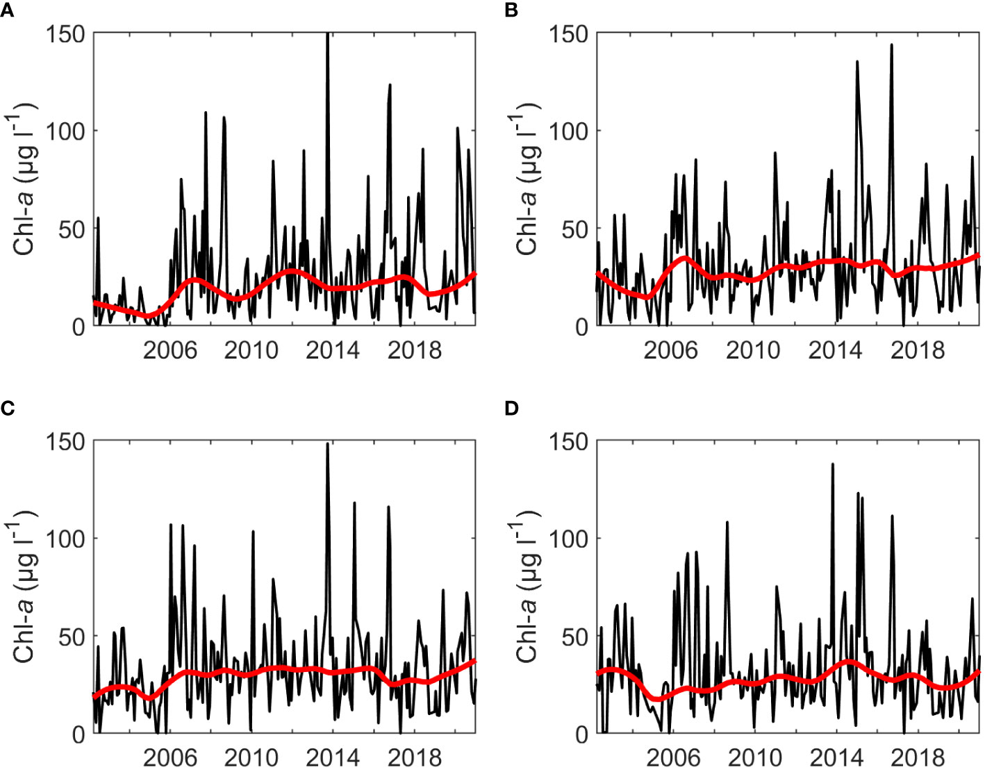
Figure 2 Monthly SWMP chl-a values (black) and fitted rloess curves (red) for the (A) Fish River, (B) Magnolia River, (C) Middle Bay, and (D) Weeks Bay stations.

FIGURE 3

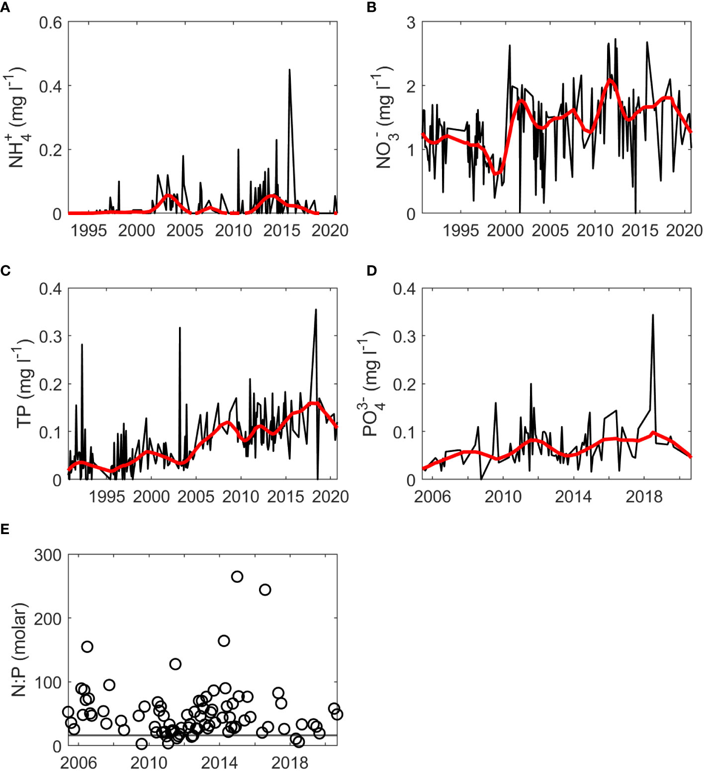
Figure 3 Monthly nutrient values (black) and fitted rloess curves (red) at the gauge for (A) NH₄⁺, (B) NO₃^-, (C) TP, (D) PO₄^3- and (E) molar N:P ratio calculated as (NH₄⁺+NO₃^-): PO₄^3-. The horizontal gray line in (E) represents the Redfield ratio. The start of time series for NH₄⁺, NO₃^-, and TP was 1990-1992 while the start of the time series for PO₄^3- was 2005.

FIGURE 4

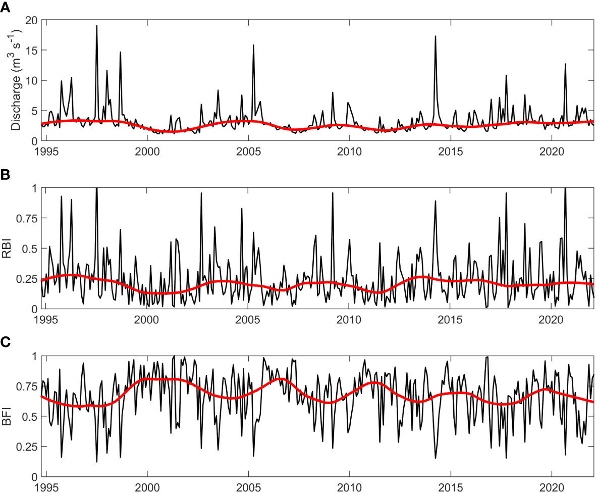
Figure 4 Hydrological variable values (black) and fitted rloess curves (red) at the gauge for (A) monthly mean discharge (m³ s^-1), (B) monthly Richards-Baker Index (RBI, unitless) and (C) monthly Baseflow Index (BFI, unitless).

TABLE 1

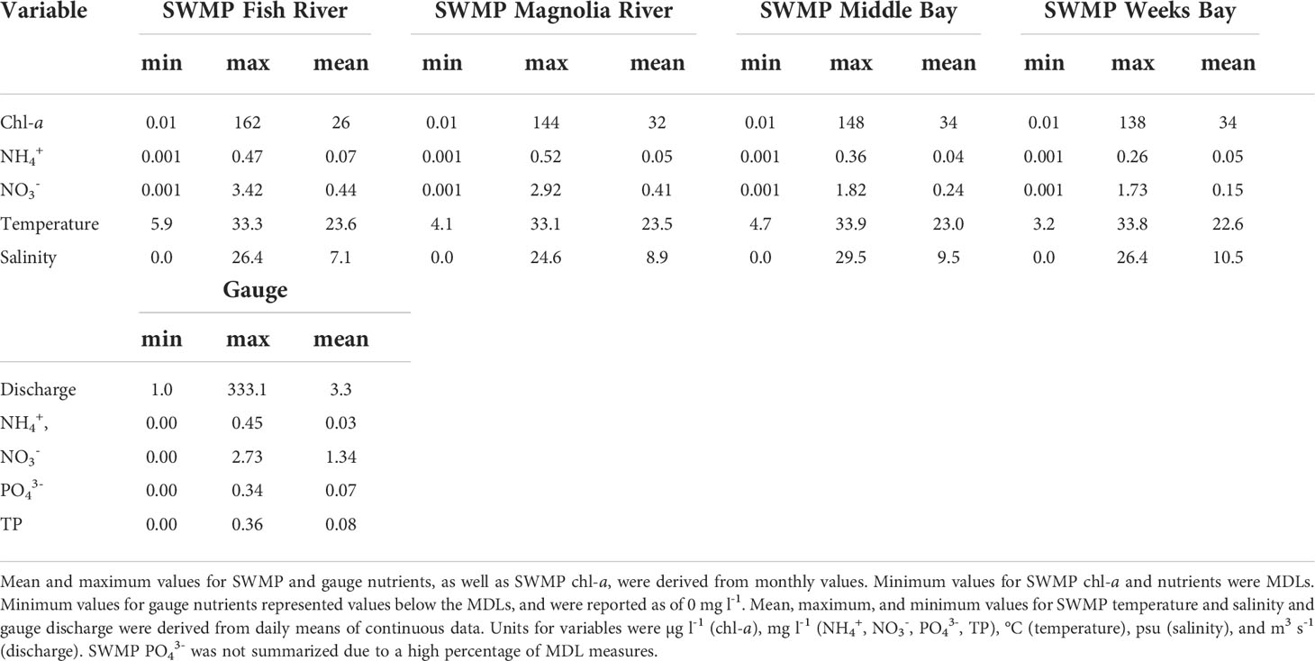
Table 1 Summary of chl-a and environmental variables.

Visual inspection also led to detection of interannual periodicity. Periodicity was identified in discharge, RBI, BFI, TP, and PO₄^3- at the gauge (Figures 3C, D, 4), in salinity, NH₄⁺, and NO₃^- at SWMP stations (Figures S3, S4), and chl-a at the SWMP Fish River station (Figure 2A). Periodicity was likely present for NH₄⁺ and NO₃^- at the gauge, but the pattern was less distinct. Presence of data gaps hindered the calculation of some period lengths in gauge TP and PO₄^3-. Nonetheless, the length of interannual periodicity for all variables appeared to follow that of discharge. Period length was approximately 8 years from the 1990s to mid-2000s. After the mid-2000s, periodicity was reduced to a length of 4 to 6 years. Interannual variability in discharge decreased after the mid-2010s, which weakened or eliminated periodicity in all variables except SWMP NH₄⁺ and chl-a. Periodicity was maintained for these two variables. The strongest periodicity in SWMP nutrients was at the river mouth stations, and the SWMP Fish River station was the only site that exhibited clear periodicity for chl-a.

Annual, seasonal, and residual decomposition

Using the multiplicative seasonal model, variables were decomposed into their annual, seasonal, and residual components. The annual component of the decompositions revealed years that were below or above average conditions. Average conditions were defined as the overall series mean. Notably, below average chl-a conditions prevailed at three of the SWMP stations until 2006, when conditions switched to above average (Figures 5A–C). Chl-a conditions were also above average in 2006 for the SWMP Weeks Bay station, but this station did not exhibit the early succession of below average years observed for the other three stations (Figure 5D). TP at the gauge similarly demonstrated a sequence of below average conditions that switched to above average conditions in the mid-2000s. The longer TP time series showed that conditions were consistently below average from 1990 to 2004, and above average for the remainder of the series (Figure 5E). Other variables at the gauge had less consistent annual patterns. Following above average conditions in the mid-1990s, RBI had nearly average conditions for the remainder of the series punctuated by 2-year periods of below average conditions (Figure 5F).

FIGURE 5

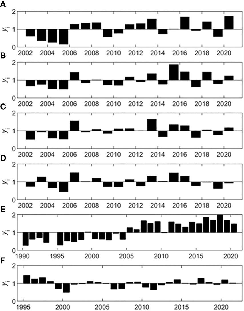
Figure 5 Annual decomposition for chl-a at the SWMP stations and TP and RBI at the gauge. The SWMP chl-a annual components (y_i, bars) are shown for the (A) Fish River, (B) Magnolia River, (C) Middle Bay, and (D) Weeks Bay stations. Gauge annual components (y_i, bars) are shown for (E) TP and (F) RBI.

The seasonal component of the decompositions represented mean monthly patterns, while the residual component represented event-based variability unexplained by annual or seasonal fluctuations. Seasonality was detected in SWMP chl-a, temperature, salinity, and NO₃^- (Figures S6, S9, S12, S18). Seasonality accounted for most of the variability in salinity and temperature. For the rest of the variables, the greatest variability was in the residual component (Table 2). Decompositions for all variables are included in the Supplementary Material (Figures S5-S26).

TABLE 2

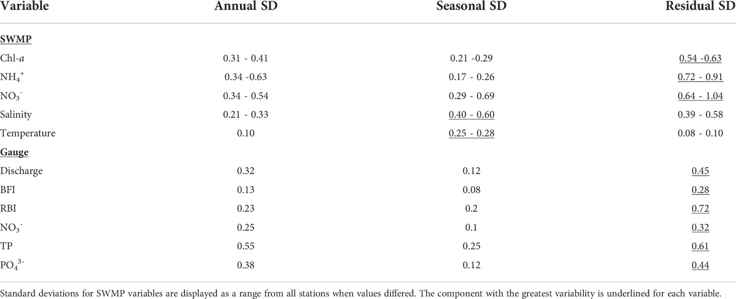
Table 2 Variability in decomposition components as the standard deviation (SD) of each component.

Monotonic and oscillating trends

Monotonic trends were identified using the Mann Kendall test on annualized data and the Seasonal Kendall test on monthly data, which removed the effect of seasonality. The rolling Seasonal Kendall test was then applied to variables with significant monotonic trends to determine if oscillations were embedded in the overall monotonic pattern.

For annualized data, the Mann Kendall test yielded significant results for three SWMP variables and one gauge variable (Table 3). Chl-a had a significant monotonic trend at the SWMP Fish River and Magnolia River stations. At the Magnolia River station, NH₄⁺ also had a significant monotonic trend. A monotonic trend was significant for temperature at the SWMP Weeks Bay station. At the gauge, TP was the only variable with a significant monotonic trend. All the trends were positive except for SWMP NH₄⁺. The strengths of the significant monotonic trends, represented by Kendall’s Tau-b (τ_b), were high for all variables. Absolute values of τ_b were > 0.3, indicating strong monotonicity. Though the variables had strong monotonicity, rates of change were low. Sen slopes were in the magnitude of 10^-3 to 10^-5.

TABLE 3

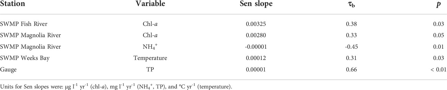
Table 3 Sen slopes and τ_b for variables with significant (p < 0.05) Mann Kendall monotonic trends at SWMP stations and the gauge.

The removal of seasonality via the Seasonal Kendall test resulted in more variables and stations with significant monotonic trends (Table 4). Chl-a at the SWMP Fish River and Magnolia River stations, temperature at the SWMP Fish River and Weeks Bay stations, salinity at the SWMP Magnolia River and Middle Bay stations, and nutrients at the gauge had significant monotonic trends. Some τ_b statistics were not as strong for the monotonic trends from monthly data as they were for yearly data. However, the Sen slopes for the Seasonal Kendall trends were considerably higher than those for the Mann Kendall trends; all slopes were in the magnitude of 10^-3 or greater. The direction of the trends was increasing for chl-a, temperature, and gauge nutrients, and decreasing for salinity.

TABLE 4

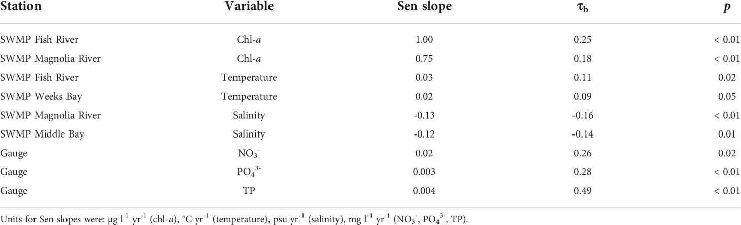
Table 4 Sen slopes and τ_b for variables with significant (p < 0.05) Seasonal Kendall monotonic trends at SWMP stations and the gauge.

The Mann Kendall and Seasonal Kendall test are proficient at identifying long-term trends that occur over the full length of the time series. However, short-term trends may also occur within the time series. These short-term trends may alternate in direction from positive to negative or vice versa, resulting in patterns that are oscillatory rather than monotonic. For variables with significant monotonic trends, we applied the rolling Seasonal Kendall test to investigate whether the data were truly monotonic over the entire course of the time series or if there were short-term oscillations within the overall monotonic pattern. Of the six variables that had significant monotonic trends, only TP at the gauge exhibited a consistent monotonic pattern (Figure 6A), though PO₄^3- at the gauge was unable to be tested due to missing monthly values. Gauge NO₃^- (data not shown) and SWMP chl-a, temperature, and salinity (data not shown) exhibited oscillations within their overall monotonic pattern. The Sen slopes for the short-term trends varied in magnitude and significance across each time series. For example, TP had four Sen slopes that were significant. All four were positive, but the steepest slope occurred in the middle of the time series (Figure 6A). Steep positive and negative slopes were seen for temperature (Figure 6B). The significant slopes for chl-a differed in timing and magnitude between the two SWMP stations. For the Fish River station, significant slopes occurred at the beginning of the time series (Figure 6C), whereas significant slopes occurred in the middle of the time series for the Magnolia River station (Figure 6D). For both stations, the significant slopes were positive and had the highest magnitude out of all the slopes calculated for each series.

FIGURE 6

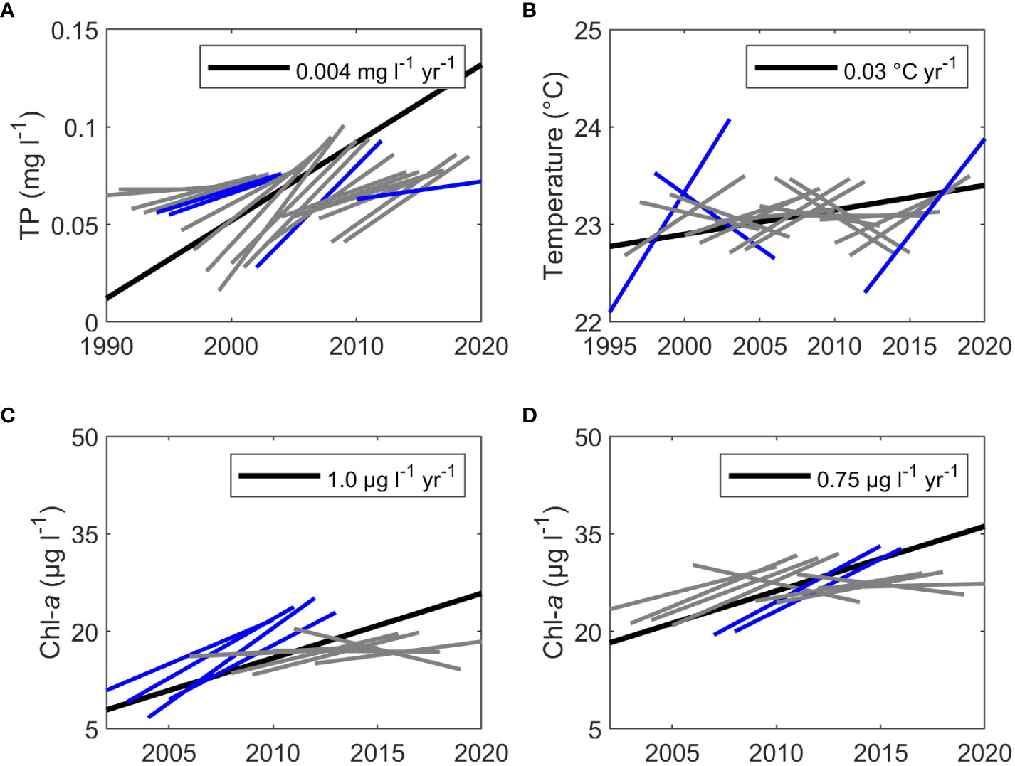
Figure 6 Sen slopes (blue and gray) of the rolling Seasonal Kendall test and the significant (p < 0.05) Seasonal Kendall monotonic Sen slopes (black) for (A) TP at the gauge, (B) temperature at the SWMP Fish River station, (C) chl-a at the SWMP Fish River station, and (D) chl-a at the SWMP Magnolia River station. Significant rolling Sen slopes (p < 0.05) are graphed in blue and non-significant rolling Sen slopes test are graphed in gray. The Seasonal Kendall Sen slope (black) is graphed to highlight differences in the long-term monotonic slope for the full time series versus the short-term rolling slopes.

Abrupt changes

Presence of abrupt changes were investigated with the Pettitt test and detected for three variables (Table 5). The change for all variables was positive. Significant abrupt changes were detected for chl-a at three SWMP stations and for two nutrients at the gauge. Chl-a change points were identified from monthly data at the SWMP Fish River, Magnolia River, and Middle Bay stations. Change periods were identified as December 2005 to January 2006 (Fish River), November 2010 to December 2010 (Magnolia River), and October 2005 to November 2005 (Middle Bay). Pettitt tests were also conducted for SWMP NH₄⁺ and NO₃^- monthly data, but no abrupt changes were detected. Missing values or strong autocorrelation prevented application of the Pettitt test on monthly data for other variables; however, the test was applied to annualized data for all variables. From annualized data, significant abrupt changes were detected for NO₃^- and TP at the gauge. Change periods for NO₃^- and TP were 1999 to 2000 and 2004 to 2005, respectively.

TABLE 5

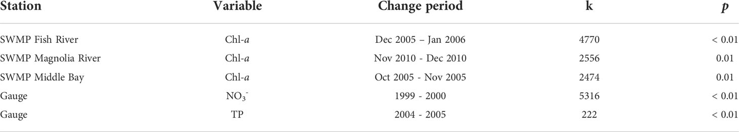
Table 5 Change dates and k statistic for variables with significant (p < 0.05) Pettitt test abrupt changes at SWMP stations and the gauge.

The abrupt changes at the three SWMP stations resulted in substantial increases in mean chl-a over the course of each time series. Calculated as the mean of annual means, overall mean chl-a at the Magnolia River station rose by 12 µg l^-1 from 2002-2010 to 2011-2020 (Figure 7A). This increase in chl-a matched the patterns observed from the rolling Seasonal Kendall test, which showed that the significant, and greatest, rates in chl-a change occurred over the 2010s (Figure 6D). At the Fish River and Middle Bay stations, overall mean chl-a rose by 21 µg l^-1 and 15 µg l^-1, respectively, from 2002-2005 to 2006-2020. However, the changes at the Fish River and Middle Bay stations occurred near the beginning of the time series, which limited the span before the increase to 4 years. To confirm that the abrupt changes were not detected as the result of a transitory period of low chlorophyll, we searched for characterizations of chl-a in Weeks Bay prior to 2002. We found independent chl-a data collected by Pennock et al. (2001) at stations across Weeks Bay from 1996 to 2000. The data were collected approximately monthly or bimonthly. Acetone extraction was used for both the Pennock et al. (2001) and the SWMP chl-a samples, which allowed comparison of measures. However, SWMP samples were collected prior to slack low tide, while the Pennock et al. (2001) collection did not target a tidal timepoint.

Two stations in the Pennock et al. (2001) data were in close vicinity to SWMP Fish River and Middle Bay stations. These were the WBAY04 station and the WBAY06 stations (Pennock et al., 2001). WBAY04 was less than 100 meters from the Fish River station and WBAY06 was less than 700 meters away from the Middle Bay station. Monthly chl-a values from the WBAY stations matched those from SWMP stations in the early 2000s (Figure 7B). When the Pennock et al. (2001) data were included in the Pettitt test for chl-a at the Fish River and Middle Bay stations, the abrupt change was still significant (p < 0.01) and the change period remained the same. Therefore, we concluded that the abrupt increase in chl-a detected at the SWMP Fish River and Middle Bay stations was a genuine abrupt change. Including the data from Pennock et al. (2001), the Fish River station, and the Middle Bay station, overall mean chl-a rose by 15 µg l^-1 from 18 µg l^-1 to 33 µg l^-1 (Figure 7C).

FIGURE 7

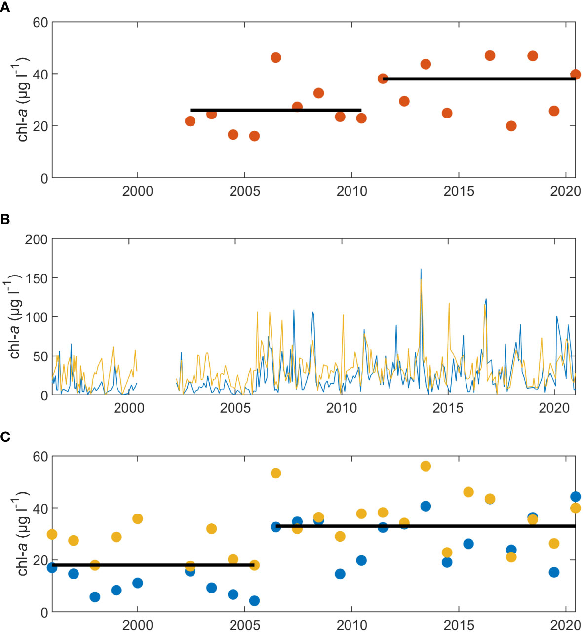
Figure 7 Representations of the abrupt chl-a change at the SWMP stations. Annual mean chl-a is shown for (A) the SWMP Magnolia River station (orange dots). Monthly chl-a values are shown in (B) for the 1996 to 2000 data (Pennock et al., 2001) and the SWMP Fish River (blue) and Middle Bay (yellow) stations. The data from 1996 to 2000 are graphed in the color of the matching SWMP station. Annual means are shown in (C) for the 1996-2000 data (blue and yellow dots) and the SWMP Fish River (blue dots) and Middle Bay (yellow dots) stations. The black horizontal lines in (A, C) represent overall mean chl-a over the indicated periods and were calculated from the annual means.

Stepwise linear regression

Based on strength of trends, the SWMP Fish River station was chosen for investigation of the relationships between chl-a and independent environmental variables using a stepwise linear regression. The predictor variables in the regression were temperature, salinity, RBI, river discharge, and nutrients at the gauge (NH₄⁺, NO₃^-, TP). SWMP nutrients were not included because they were likely to be highly impacted by and thus correlated to chl-a. Nutrients from the gauge, which were independent drivers of the estuary’s biological processes, were included. Gauge PO₄^3- was excluded due to absence of data from 2002 to 2004. BFI was excluded due to correlation with discharge (r = -0.8). Though RBI was also correlated with discharge (r = 0.8), it was included to represent frequency and duration of extreme discharge events that may have resulted in rapid flushing or long residence time of estuarine water. Collinearity was absent or weak in all other predictors.

Some data imputation was necessary to perform the regression. There were three years (2010, 2013, 2016) of missing temperature data. Data were imputed for these years by averaging the values of the previous and next year or by replacing the values with the previous year if the next year was not available. For consecutive missing values less than the length of a year, data were imputed by averaging the measures from the same date of the previous and next year. For non-consecutive missing values, data were imputed by averaging the previous and next values. Three to nine months of salinity data were missing for years 2010, 2011, and 2015. These data were imputed using an empirically derived relationship between salinity at the SWMP Fish River station and salinity at a nearby (~6 km) time series station from Alabama’s Real-Time Coastal Observing System (ARCOS)⁴ at Bon Secour (R² = 0.96). Missing nutrient data were imputed using the rloess fitted values.

Data used in the regression were from months September through December, based on the grouping of significant monthly chl-a trends (Figure S27). Predictors in the equation were transformed to z-scores, resulting in standardized coefficients. The stepwise selection procedure identified a model with three main effect variables and one interaction term that best explained the chl-a variability (Equation 3).

$$Chla= 26.8+15.9 Temp+8.3 TP-7.2 RBI+6.7 \left(Temp*TP\right)$$

(3)

Temperature had the greatest effect on variability, followed by TP, RBI, and the interaction between temperature and TP. The model had an adjusted R² of 0.34. Residuals versus fitted values did not display heteroskedasticity or violations of linearity (data not shown).

Discussion

Discrepancies in chl-a trends at the four SWMP stations demonstrated that spatial differences were significant even over an estuary as small as Weeks Bay. No chl-a trends were detected at the Weeks Bay station, while the Fish River, Magnolia River, and Middle Bay stations underwent unexpected abrupt chl-a increases. The difference in timing of these increases, combined with the lack of trends at the Weeks Bay station, suggested that the sources and magnitudes of variables influencing chl-a concentration were not equivalent across the four stations. Differential sources of chl-a drivers are reasonable given the Magnolia River and Weeks Bay station locations in the inlet of the Magnolia River and in close proximity to Mobile Bay. Conversely, the near simultaneous occurrence of the abrupt chl-a increase at the Fish River and Middle Bay stations suggested that these two sites were driven by the same conditions. Mostly likely, these conditions were the result of the Fish River and variables at the gauge.

The two variables at the gauge identified as chl-a drivers by the regression model were TP and RBI. Though temperature had a greater effect on chl-a variability, the abrupt, rather than proportional, chl-a response pointed to the crossing of a threshold. Temperature exhibited an increasing trend, but seasonal variability was greater than annual variability (Table 2). Thus, it was unlikely that a temperature threshold was crossed. In contrast, TP exhibited high annual variability, with consistently rising concentrations and an abrupt increase in 2005. We propose that this 2005 increase in phosphorus represented the exceedance of a TP threshold and resulted in the abrupt chl-a shift at the SWMP Fish River and Middle Bay stations.

The shift was likely mediated by internal phosphorus (P) loading, which is a well-established process in lakes (Pettersson, 1998; Søndergaard et al., 1999; Matisoff et al., 2016) and is also documented in estuaries (Malecki et al., 2004; Walve et al., 2018). Internal P loading refers to the amount of sedimentary P released to overlying water, and is frequently cited as the reason for delayed recovery of eutrophic lakes even after reduction of external P loading (Welch and Cooke, 2005). Sedimentary P stores are large compared to pools in the water column; thus, even small releases can have substantial effects (Pettersson, 1998). Sedimentary P retention and release varies seasonally, with retention generally occurring in the winter and release in the summer (Søndergaard et al., 1999). In lakes, anaerobic conditions are typically required to release sedimentary P, which is most often bound to metal compounds (Petticrew and Arocena, 2001). However, rates of P release are substantially elevated in hypereutrophic lakes even in the absence of stratification (Nürnberg, 1988). In coastal systems, P release does not require a deoxygenated environment (Caraco et al., 1990). The majority of microbially regenerated P is released back to the water column in marine and brackish systems, whereas freshwater regenerated P is immobilized by particle-binding and retention in the sediment (Caraco et al., 1990). Increased external P loads are known to result in increased sedimentary deposition of P, which may be further augmented in eutrophic systems by the induction of a positive feedback loop between recyclable P in organic matter and P regeneration (Carey and Rydin, 2011; Kowalczewska-Madura et al., 2015).

We hypothesize that the 2005 rise in TP built up sedimentary P stores, which resulted in a substantial increase of P released during internal loading events, triggering the upwards shift in chl-a (Figure 8) at the Fish River and Middle Bay stations. The TP threshold was estimated to be no greater than 0.10 mg l^-1, the 2005 annual mean for TP at the gauge. The occurrence of the chl-a shift in 2006, rather than 2005, was likely due to the influence of hydrology. Though the TP threshold was crossed in 2005, flashiness was average in that year. Drought conditions the following year resulted in one of the three periods of very low flashiness that occurred over the course of the discharge time series (Figure 5F). Low flashiness derived from low discharge variability would result in fewer flushing events and increased retention times, allowing biological utilization of the elevated P from internal loading. Sedimentary P stores likely remained high through the rest of time series, resupplied by still rising TP at the gauge and potential feedback loops between organic matter production and P regeneration. The tendency of internal loading to increase in the summer months may also contribute to the interaction between temperature and phosphorus in our regression model.

FIGURE 8

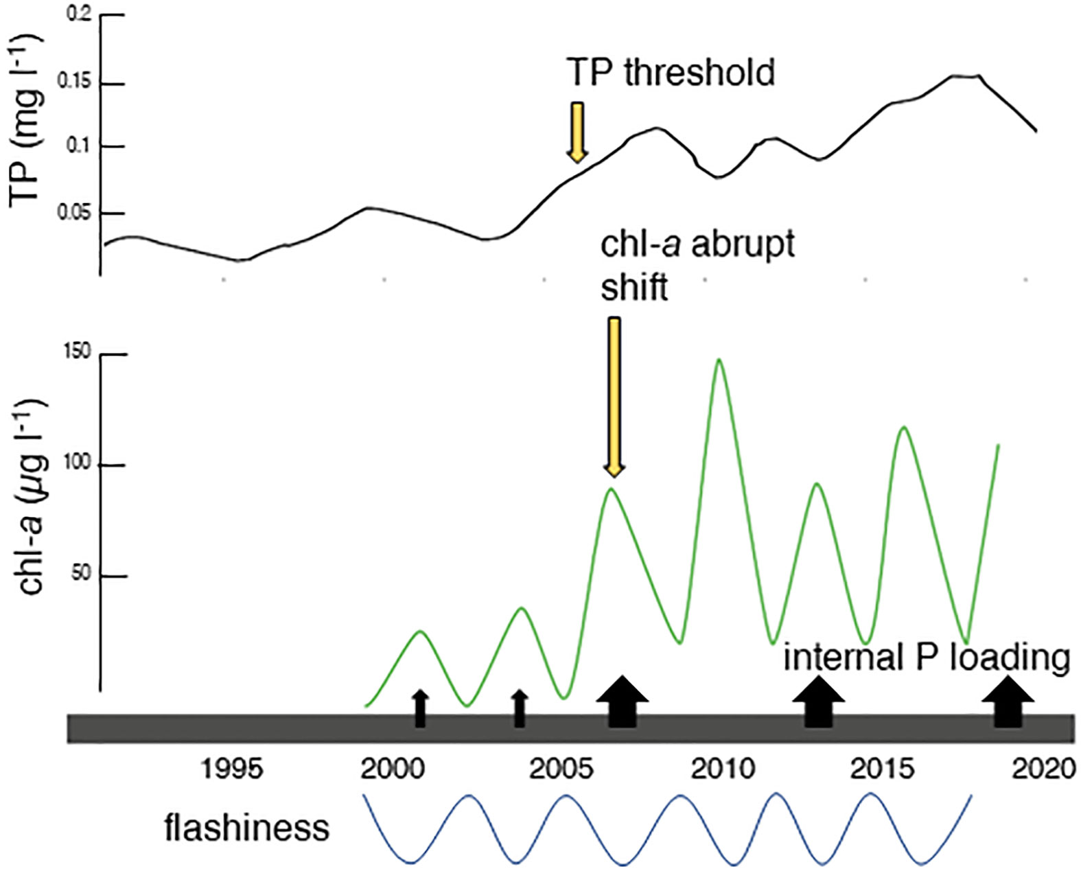
Figure 8 Conceptual diagram of the proposed mechanism behind the abrupt chl-a shift. TP is graphed on the top of the diagram (black), and is represented by the rloess curve for TP. The remainder of the variables are stylized, and do not represent true values. Chl-a (green) is graphed below TP and internal P loading is represented by black arrows. Flashiness is represented on the bottom of the graph (blue). Following the crossing of the TP threshold in 2005, sedimentary storage of P built to a level that resulted in higher internal P loading. This increased supply of phosphorus to the water column triggered the abrupt shift in 2006, when flashiness was low. Low flashiness translated to less flushing events and higher retention times, allowing the system to utilize the higher water column P released by internal loading.

The stepwise response of chl-a to phosphorus is a deviation from the generally observed relationship between chl-a and nutrients in estuaries. Though significant differences occur within and between regions, estuarine chl-a is typically thought to scale with nitrogen (Carstensen et al., 2011). However, this relationship is predominantly derived from temperate, nitrogen (N)-limited estuaries where the preponderance of estuarine research has occurred. Seasonal and spatial shifts in N- versus P-limitation have been demonstrated in estuaries such as the Chesapeake Bay (Malone et al., 1996; Prasad et al., 2010) and the Delaware Bay (Sharp et al., 2009), but nitrogen is the most common limiting nutrient in temperate coastal zones (Howarth and Marino, 2006). Consistent estuarine P-limitation may be more prevalent in warmer climates (Harrison et al., 1990; Murrell et al., 2002) and was demonstrated in Weeks Bay, where the molar N:P ratio was persistently well above the Redfield ratio. Novoveská and MacIntyre (2019) reported that the molar TN : TP ratio in the aquifer supplying groundwater to Weeks Bay exceeded 240:1, confirming the likelihood of phosphorus limitation. In this subtropical, P-limited estuary, chl-a may exhibit an altered response to phosphorus.

To our knowledge, this is the first description of a TP threshold in an estuary (Google Scholar search terms: estuar* AND threshold AND (phosphorus OR phosphate)). However, our threshold of 0.1 mg l^-1 matches with well-known phosphorus thresholds in lakes (Ibelings et al., 2007; Janse et al., 2008) where a TP concentration of 0.08 mg l^-1 to 0.12 mg l^-1 induces a shift from clear, macrophyte-dominated state to turbid, phytoplankton-dominated state (Wang et al., 2014). Whether the abrupt chl-a increase in Weeks Bay was the result of a discrete shift related to a species-specific TP threshold (Vuorio et al., 2020) or a more comprehensive change is unclear. In fresh water, shifts towards cyanobacterial dominance are often seen with increasing phosphorus concentrations (O’Neil et al., 2012), but species dominance shifts also depend on N:P ratios and competition among various phytoplankton (Zhu et al., 2010). In the absence of detailed, long-term phytoplankton composition studies that include the period of the abrupt shift, it is unlikely that the shift could be attributed to an alteration in phytoplankton community composition. The abrupt shift should instead be viewed as an overall chl-a response.

While we lacked the data to assess the cause of the chl-a increase at the SWMP Magnolia River station, the abrupt nature of the change suggests that a process similar to the one in 2006 may have occurred at this station. This hypothesis is supported by the elevated levels of chl-a observed at the Magnolia River station in 2006 (Figures 5B, 7A), which indicated that the site responded to the drivers that induced the abrupt increase at the Fish River and Middle Bay stations. Failure to maintain high chl-a concentrations may have been the result of TP concentrations in the Magnolia River that were below the proposed TP threshold. Notably, the 2011 abrupt increase in chl-a also occurred during one of the few of the years of very low Fish River flashiness (Figure 5F), which was likely mirrored in the magnitude of Magnolia River flashiness.

The non-proportional response of chl-a to phosphorus and flashiness may account for some, but not all, the variability that was not explained by the regression model. Temperature had the greatest effect on variability, and the influence of climate oscillations was suggested by the interannual periodicity in river discharge and other variables. Climate oscillations can have significant impacts on chlorophyll variability (Winder and Cloern, 2010), and river discharge in the Tombigbee-Alabama watershed has been demonstrated to be correlated with the El Niño Southern Oscillation (ENSO) and modified by the Atlantic Multidecadal Oscillation (AMO) (Dykstra and Dzwonkowski, 2021). Preliminary investigation into the impact of climate oscillations indicated relationships between ENSO and our variables, including chlorophyll and river discharge. Differences in patterns of periodicity between gauge variables and some SWMP variables, including chl-a, suggested an interesting influence of biological processes on climate oscillation effects. Other abiotic factors were not expected to significantly impact chl-a variability. In a system as shallow as Weeks Bay, the direct influence of factors such as turbidity and PAR would likely be minimized. Novoveská and MacIntyre’s (2019) study of chl-a variability in Weeks Bay from 2008 to 2010 did not identify either of these variables as correlated with chl-a, though turbidity did have an influence on phytoplankton composition.

While abiotic components underpin biology, they cannot adequately predict biological processes such as trophic cascades, species interactions, and life cycle events. Carstensen et al. (2015) found no global rules defining how phytoplankton respond to environmental variability in their meta-analysis of estuarine and coastal phytoplankton blooms and pointed to biological processes as potential site-specific regulators of phytoplankton biomass. Understanding phytoplankton phenology and interactions in the context of shifting trends in abiotic factors will likely provide additional explanatory power for biomass variability. However, achieving this level of understanding is no small task, given the dynamic nature of phytoplankton communities in natural systems.

In Weeks Bay, phytoplankton composition has been reported to fluctuate between high abundances of cryptophytes, chlorophytes, and cyanobacteria, with punctuated high concentrations of raphidophytes, dinoflagellates, and diatoms (Novoveská and MacIntyre, 2019). Temperature is known to explain the most variability in phytoplankton community composition (Bouman et al., 2003) and can provide broad community characterization. Warm periods of 30° C or greater are dominated by chroococcoid cyanobacteria, which may make up to 100% of the total chl-a in the summer months (Murrell and Caffrey, 2005). Increasing temperature is likely broadening cyanobacterial temporal range, and these species may have the additional advantages of safety from selective grazers (Leitão et al., 2018) and high affinity for phosphorus in freshwater species (Edwards et al., 2012). Novoveská and MacIntyre (2019) did not find a relationship between chl-a and phytoplankton composition, but documented three events where chl-a exceed 100 µg l^-1 and were comprised of differing phytoplankton communities. These results suggest that bloom formation is an opportunistic event in which several phytoplankton species have the potential to establish blooms. Whether a species will establish a bloom is the result of a combination of both abiotic and biotic factors. Lack of observations and knowledge regarding biological processes may limit our ability to interpret water quality monitoring data, which generally do not include biological measures beyond chl-a.

While we were not able to fully explain the variability in chlorophyll, the decadal nature of the NERRS SWMP data sets allowed detection of long-term trends and an abrupt shift in chl-a concentration. The abrupt shift opposed our hypothesis that chl-a would follow an increasing trend that matched the nutrient trend; however, positive temperature and negative hydrology effects were evident. Studies that present sufficient evidence for abrupt change are rare. The long-term chlorophyll time series from San Francisco Bay provides one of the only well-characterized examples of an abrupt increase in estuarine phytoplankton biomass (Cloern et al., 2007), though abrupt decreases in phytoplankton biomass due to climactic forcings or trophic cascades have also been documented (Strayer et al., 2008; Borkman and Smayda, 2009). Because the Magnolia River’s influence over the SWMP Magnolia River station was likely greater than the influence of the Fish River, we were unable to identify a driver that induced the chl-a increase and therefore could not define the increase as an abrupt shift. We were able to define the increases at the SWMP Fish River and Middle Bay stations as an abrupt shift. Analysis of the increases at these two stations overcame the four major impediments listed by Mac Nally et al. (2014) for the detection of stark change. Firstly, the shift was clearly specified as a statistically significant change in chl-a concentration, an ecosystem response. Secondly, we identified the abrupt shift from a true time series, rather than from only two points in time or from space for time substitution. Thirdly, the length of the time series enabled confirmation that the abrupt shift was a unique, rather than periodic, event. Lastly, the data utilized in the analysis included contemporaneous measures of variables that were potential drivers of chlorophyll variability; thus, we were able to link the abrupt shift in chl-a to changes in phosphorus and hydrology.

Data availability statement

Publicly available datasets were analyzed in this study. This data can be found here: Centralized Data Management Office of the NERRS at cdmo.baruch.sc.edu, The Water Quality Portal at waterqualitydata.us, USGS waterdata.usgs.gov, ARCOS arcos.disl.org, Pennock et al. (2001).

Author contributions

MF: Conceptualization, Methodology, Validation, Formal analysis, Writing – Original Draft, Writing – Review and Editing. SP: Investigation, Resources, Data Curation, Supervision. JL: Conceptualization, Methodology, Writing – Review and Editing, Supervision. All authors contributed to the article and approved the submitted version.

Funding

This paper is a result of research funded by the National Oceanic and Atmospheric Administration’s Margaret A. Davidson Fellowship (NA20NOS4200120) and the RESTORE Science Program (NOAA RESTORE NA19NOS4510194) under awards to the University of South Alabama.

Acknowledgments

We would like the acknowledge the staff at the Weeks Bay NERR. Their dedication to the reserve and continued maintenance of the SWMP made this work possible.

Conflict of interest

The authors declare that the research was conducted in the absence of any commercial or financial relationships that could be construed as a potential conflict of interest.

Publisher’s note

All claims expressed in this article are solely those of the authors and do not necessarily represent those of their affiliated organizations, or those of the publisher, the editors and the reviewers. Any product that may be evaluated in this article, or claim that may be made by its manufacturer, is not guaranteed or endorsed by the publisher.

Supplementary material

The Supplementary Material for this article can be found online at: https://www.frontiersin.org/articles/10.3389/fmars.2022.990404/full#supplementary-material

Footnotes

1. ^ cdmo.baruch.sc.edu.
2. ^ waterqualitydata.us.
3. ^ waterdata.usgs.gov.
4. ^ arcos.disl.org.

References

ADEM (2014). 2014 Alabama integrated water quality monitoring and assessment report (Montgomery, AL: Alabama Department of Environmental Management).

Google Scholar

APHA (1998). Standard methods for the examination of water and wastewater. 20th Edition (Washington DC: American Health Association).

Google Scholar

Auber A., Travers-Trolet M., Villanueva M. C., Ernande B. (2015). Regime shift in an exploited fish community related to natural climate oscillations. PLoS One 10, e0129883. doi: 10.1371/journal.pone.0129883

PubMed Abstract | CrossRef Full Text | Google Scholar

Baker D. B., Richards R. P., Loftus T. T., Kramer J. W. (2004). A new flashiness index: characteristics and applications to midwestern rivers and streams. J. Am. Water Resour. Assoc. 40, 503–522. doi: 10.1111/j.1752-1688.2004.tb01046.x

CrossRef Full Text | Google Scholar

Baumann H., Smith E. M. (2017). Quantifying metabolically driven pH and oxygen fluctuations in US nearshore habitats at diel to intereannual time scales. Estuaries Coasts 41, 1102–1117. doi: 10.1007/s12237-017-0321-3

CrossRef Full Text | Google Scholar

Borkman D. G., Smayda T. (2009). Multidecadal 1959-1997) changes in skeletonema abundance and seasonal bloom patterns in Narragansett bay, Rhode island, USA. J. Sea Res. 61, 84–94. doi: 10.1016/j.seares.2008.10.004

CrossRef Full Text | Google Scholar

Borsuk M. E., Stow C. A., Reckhow K. H. (2004). Confounding effect of flow on estuarine response to nitrogen loading. J. Environ. Eng. 130, 605–614. doi: 10.1061/(ASCE)0733-9372(2004)130:6(605

CrossRef Full Text | Google Scholar

Bouman H. A., Platt T., Sathyendranath S., Li W. K. W., Stuart V., Fuentes-Yaco C., et al. (2003). Temperature as indicator of optical properties and community structure of marine phytoplankton: implications for remote sensing. Mar. Ecol. Prog. Ser. 258, 19–30. doi: 10.3354/meps258019

CrossRef Full Text | Google Scholar

Boyer J. N., Kelble C. R., Ortner P. B., Rudnick D. T. (2009). Phytoplankton bloom status: Chlorophyll a biomass as an indicator of water quality condition in the southern estuaries of Florida, USA. Ecol. Indic. 9, S56–S67. doi: 10.1016/j.ecolind.2008.11.013

CrossRef Full Text | Google Scholar

Breton E., Brunet C., Sautour B., Brylinski J. (2000). Annual variations of phytoplankton biomass in the Eastern English channel: comparison by pigment signatures and microscopic counts. J. Plankton Res. 22, 1423–1440. doi: 10.1093/plankt/22.8.1423

CrossRef Full Text | Google Scholar

Burkey J. (2022a). Homogeneity test of global trends using chi-square on Mann-Kendall. Available at: https://www.mathworks.com/matlabcentral/fileexchange/22440-homogeneity-test-of-global-trends-using-chi-square-on-mann-kendall (Accessed March 1, 2022).

Google Scholar

Burkey J. (2022b). Mann-Kendall Tau-b with sen’s method (enhanced). Available at: https://www.mathworks.com/matlabcentral/fileexchange/11190-mann-kendall-tau-b-with-sen-s-method-enhanced (Accessed March 1, 2022).

Google Scholar

Burkey J. (2022c). Seasonal Kendall test with slope for serial dependent data. Available at: https://www.mathworks.com/matlabcentral/fileexchange/22389-seasonal-kendall-test-with-slope-for-serial-dependent-data (Accessed March 1, 2022).

Google Scholar

Canion A., MacIntyre H. L., Phipps S. (2013). Short-term to seasonal variability in factors driving primary productivity in a shallow estuary: Implications for modeling production. Estuar. Coast. Shelf Sci. 131, 224–234. doi: 10.1016/j.ecss.2013.07.009

CrossRef Full Text | Google Scholar

Capon S. J., Jasmyn Lynch A. J., Chessman B. C., Davis J., Finlayson M., Hohnberg D., et al. (2015). Regime shifts, thresholds and multiple stable states in freshwater ecosystems; a critical appraisal of the evidence. Sci. Total Environ. 534, 122–130. doi: 10.1016/j.scitotenv.2015.02.045

PubMed Abstract | CrossRef Full Text | Google Scholar

Caraco N., Cole J., Likes G. (1990). A comparison of phosphorus immobilization in sediments of freshwater and coastal marine systems. Biogeochemistry 9, 277–290. doi: 10.1007/bf00000602

CrossRef Full Text | Google Scholar

Carey C. C., Rydin E. (2011). Lake trophic status can be determined by the depth distribution of sediment phosphorus. Limnol. Oceanogr. 56, 2051–2063. doi: 10.4319/lo.2011.56.6.2051

CrossRef Full Text | Google Scholar

Carstensen J., Klais R., Cloern J. E. (2015). Phytoplankton blooms in estuarine and coastal waters: Seasonal patterns and key species. Estuar. Coast. Shelf Sci. 162, 98–109. doi: 10.1016/j.ecss.2015.05.005

CrossRef Full Text | Google Scholar

Carstensen J., Sánchez-Camacho M., Duarte C. M., Krause-Jensen D., Marbà N. (2011). Connecting the dots: Responses of coastal ecosystems to changing nutrient concentrations. Environ. Sci. Technol. 45, 9122–9132. doi: 10.1021/es202351y

PubMed Abstract | CrossRef Full Text | Google Scholar

Charpentier A., Grillas P., Lescuyer F., Coulet E., Auby I. (2005). Spatio-temporal dynamics of a zostera noltii dominated community over a period of fluctuating salinity in a shallow lagoon, southern France. Estuar. Coast. Shelf Sci. 64, 307–315. doi: 10.1016/j.ecss.2005.02.024

CrossRef Full Text | Google Scholar

Chen M., Daroub S. H., Nadal V. (2006). Comparison of two digestion methods for determining total phosphorus in farm canal water. Commun. Soil Sci. Plant Anal. 37, 2351–2363. doi: 10.1080/00103620600819842

CrossRef Full Text | Google Scholar

Cloern J. E. (2019). Patterns, pace, and processes of water-quality variability in a long-studied estuary. Limnol. Ocean. 64, S192–S208. doi: 10.1002/lno.10958

CrossRef Full Text | Google Scholar

Cloern J. E., Hieb K. A., Jacobson T., Sansó B., Di Lorenzo E., Stacey M. T., et al. (2010). Biological communities in San Francisco bay track large-scale climate forcing over the north pacific. Geophys. Res. Lett. 37. doi: 10.1029/2010GL044774

CrossRef Full Text | Google Scholar

Cloern J. E., Jassby A. D. (2010). Patterns and scales of phytoplankton variability in estuarine-coastal ecosystems. Estuaries Coasts 33, 230–241. doi: 10.1007/s12237-009-9195-3

CrossRef Full Text | Google Scholar

Cloern J. E., Jassby A. D., Thompson J. K., Hieb K. A. (2007). A cold phase of the East pacific triggers new phytoplankton blooms in San Francisco bay. Proc. Natl. Acad. Sci. 104, 18561–18565. doi: 10.1073/pnas.070615110

CrossRef Full Text | Google Scholar

Cole B. E., Cloern J. E. (1987). An empirical model for estimating phytoplankton productivity in estuaries. Artic. Mar. Ecol. Prog. Ser. 36, 299–305. doi: 10.3354/meps036299

CrossRef Full Text | Google Scholar

Daskalov G. M. (2002). Overfishing drives a trophic cascade in the black Sea. Mar. Ecol. Prog. Ser. 225, 53–63. doi: 10.3354/meps225053

CrossRef Full Text | Google Scholar

Dey P. (2022). Pettitt change point test for univariate time series data. Available at: https://www.mathworks.com/matlabcentral/fileexchange/60973-pettitt-change-point-test-for-univariate-time-series-data (Accessed March 1, 2022).

Google Scholar

Dykstra S. L., Dzwonkowski B. (2021). The role of intensifying precipitation on coastal river flooding and compound river-storm surge events, northeast gulf of Mexico. Water Resour. Res. 57, e2020WR029363. doi: 10.1029/2020WR029363

PubMed Abstract | CrossRef Full Text | Google Scholar

Edwards K. F., Thomas M. K., Klausmeier C. A., Litchman E. (2012). Allometric scaling and taxonomic variation in nutrient utilization traits and maximum growth rate of phytoplankton. Limnol. Ocean. 57, 554–566. doi: 10.4319/lo.2012.57.2.0554

CrossRef Full Text | Google Scholar

Geider R. J., MacIntyre H. L., Kana T. M. (1997). Dynamic model of phytoplankton growth and acclimation: responses of the balanced growth rate and the chlorophyll a: carbon ratio to light, nutrient-limitation, and temperature. Mar. Ecol. Prog. Ser. 148, 187–2000. doi: 10.3354/meps148187

CrossRef Full Text | Google Scholar

Gustard A., Bullock A., Dixon J. M. (1992). Low flow estimation in the united kingdom (Wallingford, Oxfordshire, UK:Institute of Hydrology).

Google Scholar

Harrison P. J., Hu M. H., Yang Y. P., Lu X. (1990). Phosphate limitation in estuarine and coastal waters of China. J. Exp. Mar. Bio. Ecol. 140, 79–87. doi: 10.1016/0022-0981(90)90083-O

CrossRef Full Text | Google Scholar

Hewitt J. E., Thrush S. F. (2010). Empirical evidence of an approaching alternate state produced by intrinsic community dynamics, climatic variability and management actions. Mar. Ecol. Prog. Ser. 413, 267–276. doi: 10.3354/meps08626

CrossRef Full Text | Google Scholar

Howarth R. W., Marino R. (2006). Nitrogen as the limiting nutrient for eutrophication in coastal marine ecosystems : Evolving views over three decades. Limnol. Ocean. 51, 364–376. doi: 10.4319/lo.2006.51.1_part_2.0364

CrossRef Full Text | Google Scholar

Ibelings B. W., Portielje R., Lammens E. H. R. R., Noordhuis R., Van Den Berg M. S., Joosse W., et al. (2007). Resilience of alternative stable states during the recovery of shallow lakes from eutrophication: Lake veluwe as a case study. Ecosystems 10, 4–16. doi: 10.1007/s10021-006-9009-4

CrossRef Full Text | Google Scholar

Janse J. H., De Senerpont Domis L. N., Scheffer M., Lijklema L., Van Liere L., Klinge M., et al. (2008). Critical phosphorus loading of different types of shallow lakes and the consequences for management estimated with the ecosystem model PCLake. Limnologica 38, 203–219. doi: 10.1016/j.limno.2008.06.001

CrossRef Full Text | Google Scholar

Kowalczewska-Madura K., Gołdyn R., Dera M. (2015). Spatial and seasonal changes of phosphorus internal loading in two lakes with different trophy. Ecol. Eng. 74, 187–195. doi: 10.1016/j.ecoleng.2014.10.033

CrossRef Full Text | Google Scholar

Lees K., Pitois S., Scott C., Frid C., Mackinson S. (2006). Characterizing regime shifts in the marine environment. Fish. Fish. 7, 104–127. doi: 10.1111/j.1467-2979.2006.00215.x

CrossRef Full Text | Google Scholar

Lehman P. W. (2000). The influence of climate on phytoplankton community biomass in San Francisco bay estuary. Limnol. Oceanogr. 45, 580–590. doi: 10.4319/lo.2000.45.3.0580

CrossRef Full Text | Google Scholar

Lehrter J. C. (2006). Effects of land use and land cover, stream discharge, and interannual climate on the magnitude and timing of nitrogen, phosphorus, and organic carbon concentrations in three coastal plain watersheds. Water Environ. Res. 78, 2356–2368. doi: 10.2175/106143006x102015

PubMed Abstract | CrossRef Full Text | Google Scholar

Lehrter J. C. (2008). Regulation of eutrophication susceptibility in oligohaline regions of a northern gulf of Mexico estuary, mobile bay, Alabama. Mar. pollut. Bull. 56, 1446–1460. doi: 10.1016/j.marpolbul.2008.04.047

PubMed Abstract | CrossRef Full Text | Google Scholar

Leitão E., Ger K. A., Panosso R. (2018). Selective grazing by a tropical copepod (Notodiaptomus iheringi) facilitates microcystis dominance. Front. Microbiol. 9. doi: 10.3389/fmicb.2018.00301

PubMed Abstract | CrossRef Full Text | Google Scholar

Mac Nally R., Albano C., Fleishman E. (2014). A scrutiny of the evidence for pressure-induced state shifts in estuarine and nearshore ecosystems. Austral Ecol. 39, 898–906. doi: 10.1111/aec.12162

CrossRef Full Text | Google Scholar

Malecki L. M., White J. R., Reddy K. R. (2004). Wetlands and aquatic processes. J. Environ. Qual. 33, 1545–1555. doi: 10.2134/jeq2004.1545

PubMed Abstract | CrossRef Full Text | Google Scholar

Malone T., Conley D. J., Fisher T. R., Gilbert P. M., Harding L. W., Sellner K. G. (1996). Scales of nutrient-limited phytoplankton productivity in Chesapeake bay. Estuaries 19, 371–385. doi: 10.2307/1352457

CrossRef Full Text | Google Scholar

Matisoff G., Kaltenberg E. M., Steely R. L., Hummel S. K., Seo J., Gibbons K. J., et al. (2016). Internal loading of phosphorus in western lake Erie. J. Great Lakes Res. 42, 775–788. doi: 10.1016/j.jglr.2016.04.004

CrossRef Full Text | Google Scholar

Miller-Way T., Dardeau M., Crozier G. (1996). Weeks bay national estuarine research reserve: An estuarine profile and bibliography. Dauphin Island Sea Lab. Tech. Rep., 96–01. (Dauphin Island, AL.)

Google Scholar

Mortazavi B., Riggs A. A., Caffrey J. M., Genet H., Phipps S. W. (2012). The contribution of benthic nutrient regeneration to primary production in a shallow eutrophic estuary, weeks bay, Alabama. Estuaries Coasts 35, 862–877. doi: 10.1007/s12237-012-9478-y

CrossRef Full Text | Google Scholar

Murrell M. C., Caffrey J. M. (2005). High cyanobacterial abundance in three northeastern gulf of Mexico estuaries. Gulf Caribb. Res. 17, 95–106. doi: 10.18785/gcr.1701.08

CrossRef Full Text | Google Scholar

Murrell M. C., Stanley R. S., Lores E. M., DiDonato G. T., Smith L. M., Flemer D. A. (2002). Evidence that phosphorus limits phytoplankton growth in a gulf of Mexico estuary: Pensacola bay, Florida, USA. Bull. Mar. Sci. 70, 155–167.

Google Scholar

Novoveská L., MacIntyre H. L. (2019). Study of the seasonality and hydrology as drivers of phytoplankton abundance and composition in a shallow estuary, weeks bay, Alabama (USA). J. Aquac. Mar. Biol. 8, 69–80. doi: 10.15406/jamb.2019.08.00245

CrossRef Full Text | Google Scholar

Nürnberg G. K. (1988). Prediction of phosphorus release rates from ttotal reductant-soluble phosphorus in anoxic lake sediments. Can. J. Fish. Aquat. Sci. 45, 453–462. doi: 10.1139/f88-054

CrossRef Full Text | Google Scholar

O’Neil J. M., Davis T. W., Burford M. A., Gobler C. J. (2012). The rise of harmful cyanobacteria blooms: the potential roles of eutrophication and climate change. Harmful Algae 14, 313–334. doi: 10.1016/j.hal.2011.10.027

CrossRef Full Text | Google Scholar

Patton C. J., Truitt E. P. (1992). Methods of analysis by the U.S. geological survey national water quality laboratory–determination of total phosphorus by a kjeldahl digestion method and an automated colorimetric finish that includes dialysis. U.S. Geol. Surv. Open-File Rep. 92-146 92. doi: 10.3133/ofr92146

CrossRef Full Text | Google Scholar

Pennock J., Cowan J., Shotts K., Cowan J., LJ G. (2001). Weeks Bay data report: WBAY-2 to WBAY56 cruises (May 1996-May 2000). (Dauphin Island, AL.:Dauphin Island Sea Lab Technical Report 1)

Google Scholar

Pennock J. R., Sharp J. H. (1986). Phytoplankton production in the Delaware estuary: temporal and spatial variability. Mar. Ecol. Prog. Ser. 34, 143–155. doi: 10.3354/meps034143

CrossRef Full Text | Google Scholar

Pettersson K. (1998). Mechanisms for internal loading of phosphorus in lakes. Hydrobiologia, 373, 21–25. doi: 10.1007/978-94-011-5266-2_2

CrossRef Full Text | Google Scholar

Petticrew E. L., Arocena J. M. (2001). Evaluation of iron-phosphate as a source of internal lake phosphorus loadings. Sci. Total Environ. 266, 87–93. doi: 10.1016/S0048-9697(00)00756-7

PubMed Abstract | CrossRef Full Text | Google Scholar

Prasad M. B. K., Sapiano M. R. P., Anderson C. R., Long W., Murtugudde R. (2010). Long-term variability of nutrients and chlorophyll in the Chesapeake bay: A retrospective analysis 1985-2008. Estuaries Coasts 33, 1128–1143. doi: 10.1007/s12237-010-9325-y

CrossRef Full Text | Google Scholar

Søndergaard M., Jensen J. P., Jeppesen E. (1999). Internal phosphorus loading in shallow Danish lakes. Hydrobiologia 408–409, 145–152. doi: 10.1007/978-94-017-2986-4_15

CrossRef Full Text | Google Scholar

Sharp J. H., Yoshiyama K., Parker A. E., Schwartz M. C., Curless S. E., Beauregard A. Y., et al. (2009). A biogeochemical view of estuarine eutrophication: Seasonal and spatial trends and correlations in the Delaware estuary. Estuaries Coasts 32, 1023–1043. doi: 10.1007/s12237-009-9210-8

CrossRef Full Text | Google Scholar

Smith V. H., Schindler D. W. (2009). Eutrophication science: where do we go from here? Trends Ecol. Evol. 24, 201–207. doi: 10.1016/j.tree.2008.11.009

PubMed Abstract | CrossRef Full Text | Google Scholar

Strayer D. L., Pace M. L., Caraco N. F., Cole J. J., Findlay S. E. (2008). Hydrology and grazing jointly control a large-river food web. Ecology 89, 12–18. doi: 10.1890/07-0979.1

PubMed Abstract | CrossRef Full Text | Google Scholar

Tetra Tech Inc (2013). Sources, fate, transport, and effects (SFTE) of nutrients as a basis for protective criteria in estuarine and near-coastal waters, (Weeks Bay, Alabama pilot study:Owings Mills, MD).

Google Scholar

Thompson Engineering (2017). Final weeks bay watershed management plan. project no. 16-1101-0012 (Mobile, AL: Mobile Bay National Estuary Program).

Google Scholar

Vuorio K., Järvinen M., Kotamäki N. (2020). Phosphorus thresholds for bloom-forming cyanobacterial taxa in boreal lakes. Hydrobiologia 847, 4389–4400. doi: 10.1007/s10750-019-04161-5

CrossRef Full Text | Google Scholar

Walve J., Sandberg M., Larsson U., Lännergren C. (2018). A Baltic Sea estuary as a phosphorus source and sink after drastic load reduction: Seasonal and long-term mass balances for the Stockholm inner archipelago for 1968-2015. Biogeosciences 15, 3003–3025. doi: 10.5194/bg-15-3003-2018

CrossRef Full Text | Google Scholar

Wang H.-J., Wang H.-Z., Liang X.-M., Wu S.-K. (2014). Total phosphorus thresholds for regime shifts are nearly equal in subtropical and temperate shallow lakes with moderate depths and areas. Freshw. Biol. 59, 1659–1671. doi: 10.1111/fwb.12372

CrossRef Full Text | Google Scholar

Welch E. B., Cooke G. D. (2005). Internal phosphorus loading in shallow lakes: Importance and control. Lake Reserv. Manage. 21, 209–217. doi: 10.1080/07438140509354430

CrossRef Full Text | Google Scholar

Winder M., Cloern J. E. (2010). The annual cycles of phytoplankton biomass. Philos. Trans. R. Soc B Biol. Sci. 365, 3215–3226. doi: 10.1098/rstb.2010.0125

CrossRef Full Text | Google Scholar

Zhu W., Wan L., Zhao L. (2010). Effect of nutrient level on phytoplankton community structure in different water bodies. J. Environ. Sci. 22, 32–39. doi: 10.1016/S1001-0742(09)60071-1

CrossRef Full Text | Google Scholar