On the control of spatial and temporal oceanic scales by existing and future observing systems: An observing system simulation experiment approach

1 Introduction

As the ocean plays a fundamental role in regulating climate variability, it has been recognized in the 1980-90’s that systematic ocean observations are essential to understand and monitor the changing climate of the Earth (e.g., Fu et al., 1994; McPhaden et al., 1998). Initially focused on capturing oceanic variability at large spatial McPhaden et al., 1998, the scope of sustained ocean observations is now expanded to serve diverse end-users, with multi-scale sampling and multi-disciplinary needs (Moltmann et al., 2019). These observations are integrated in the global ocean observing system (GOOS), which includes data stream from satellites and in situ platforms. These strong efforts have been essential for the development of ocean models and data assimilation methods allowing to validate and optimize numerical simulations (Smith, 1993). Given these different sources of ocean information from satellites, in situ platforms and assimilative models, the Global Ocean Data Assimilation Experiment (GODAE) has strongly supported the implementation of global ocean analysis and forecasting capabilities for operational oceanography (Cummings et al., 2009; Bell et al., 2015). The objective was to build operational systems able to provide to the scientific and broader communities the most accurate estimates of essential physical oceanic variables.

Over the last three decades, significant progress has been made in model developments and data assimilation techniques (Moore et al., 2019), and the diversity of assimilated in situ platforms is steadily increasing (Tanhua et al., 2019). Yet, given the complexity of operational systems, it is not currently possible to easily establish the efficiency of the various observations in constraining the ocean state, and to determine how information from observations is used. It also becomes more and more difficult to evaluate the influence of a change in the observing system on ocean analyses, which would be essential to determine the utility and relevance of such changes from the integrated ocean observing system perspective.

Numerous studies based on numerical experiments have investigated the impact of existing or future in situ observations in ocean analysis and forecasting systems (Fujii et al., 2019). For instance, the complementarity between tropical mooring, Argo and altimetry data has been demonstrated for global ocean analysis (Balmaseda et al., 2007; Turpin et al., 2016) and seasonal forecasting (Balmaseda and Anderson, 2009; Balmaseda et al., 2013; Fujii et al., 2015). Other studies have also focused on specific regions, like the Tropical Pacific (e.g., Zhu et al., 2021), the Australian coast (e.g., Jones et al., 2012; Aydogdu et al., 2016), or the abyssal Ocean (e.g., Gasparin et al., 2020; Levin et al., 2021). However, a large part of impact studies was dedicated to existing in situ observations and/or did not consider the integrated value of the global ocean observing system (e.g., no assimilation of altimetry; Fujii et al., 2019). In addition, usual evaluation metrics, mostly based on box-averaged statistics, make it difficult to separate observation impacts depending on specific space and temporal scales.

The purpose of the present study is thus to analyze the impact of in situ observations on constraining oceanic analyses/reanalyses based on Observing System Simulation Experiments (OSSEs), considering both satellites and in situ observations and their complementarity or redundancy. A first objective is to disentangle the added value of in situ observations when satellite data are already assimilated, while a second objective is to determine their respective ability to constrain specific temporal and spatial scales. Special attention is given to the evaluation of international recommendations for the Argo array and the tropical moored array. Our results will illustrate the need for continuing assessments and improvements of data assimilation techniques for in situ observations and should pave the way for future operational systems improvements to increase benefits of ocean observations.

The paper is organized as follows. In the next section, the methodology based on numerical experiments is described. In Section 3, the added value of the main components of the ocean observing system is presented. Section 4 discusses potential outcomes of enhancements of the in situ observing system in western boundary current regions and in tropical basins. Discussion and conclusion are provided in Section 5.

2 Data and methodology

The present study is based on a comparison of a series of numerical experiments, called observing system simulation experiments (OSSEs), in which different designs of ocean observations have been assimilated. The present work follows the OSSEs best practices proposed by Halliwell et al. (2014) as much as possible. The OSSEs ingredients are (i) an unconstrained simulation, named the Nature Run, assumed to provide a good representation of the “true” ocean variability over the space and time scales of interest, (ii) a set of synthetic realistic observations simulating different observing system designs, generated from the Nature Run, and (iii) a global experimental system assimilating the above synthetic observations.

2.1 Modelling components

The Nature Run corresponds to the free-running version (i.e., without data assimilation) of the GLORYS12 reanalysis at 1/12° horizontal resolution (Lellouche et al., 2021), called FREEGLORYS12. This unconstrained simulation has been developed at Mercator Ocean International and is based on the NEMO3.1 ocean model (Madec and The NEMO Team, 2008), using a 1/12° ORCA grid (horizontal resolution of 9 km at the equator, 7 km at mid-latitudes and 2 km near the poles). The ocean model is forced at the surface with the atmospheric fields from the ERA-Interim reanalysis produced by the European Centre for Medium-Range Weather Forecasts (ECMWF) (Dee et al., 2011). The Nature Run was initialized in October 1991, from the EN4 gridded fields of temperature and salinity (Good et al., 2013). Assuming that the ocean is initially at rest, the model physics then spins up a velocity field in balance with the density field after about 1 year. The Nature Run was run up until the end of 2017, during which the 2015-2017 period was used to generate synthetic observations.

The experimental analysis system used to perform OSSEs is based on the global Mercator Ocean operational system to be deployed in the Copernicus Marine Service (see Le Traon et al., 2019) portfolio by the end of 2022. The ocean model uses version 3.6 of NEMO (Madec et al., 2017) with a ¼° ORCA grid type (Madec and Imbard, 1996), and is forced at the surface by the operational atmospheric fields from the ECMWF-Integrated Forecast System (ECMWF-IFS) with 3-h resolution. A coherent bulk formulation is derived from the IFS model (Brodeau et al., 2017), but no atmospheric pressure forcing is used. Moreover, the surface currents are not considered in the stress computation (absolute wind) as it was the case for the Nature Run. The ocean model uses an explicit barotropic mode solved by a split-explicit approach (Shchepetkin and McWilliams, 2005), a second order vertical mixing (k-espilon; Rodi, 1987) and a UBS scheme (Shchepetkin and McWilliams, 2008) for computing the horizontal momentum advection without addition of an explicit diffusion.

In addition to the ocean model, the assimilative system consists of a 3D-Var bias correction for the slowly evolving large-scale biases in temperature and salinity, and a local version of a reduced-order Kalman filter based on the Singular Evolutive Extended Kalman filter formulation (Brasseur and Verron, 2006). In practice, temperature and salinity observations are selected depending on the innovation value, defined as the observation minus model forecast equivalent. For the 3D-Var corrections, innovations are considered on a temporal window of 1 month (i.e., at a given 7-day cycle and the three previous cycles) and on spatial window of the order of 400–500 km in order to map large-scale temperature and salinity corrections. For the assimilation of the SEEK filter, the analysis at a given point is based on surrounded innovations determined by spatial and temporal correlation scales, ranging from 50 to 450 km in the zonal direction, from 50 to 200 km in the meridional direction and from 3 to 15 days. From the innovations and specified observation errors, the SEEK filter generates a localized analysis increment, which is a linear combination of short-scale anomalies from a statistical ensemble representative of the forecast error covariances (Lellouche et al., 2013). The 3D-Var correction and the SEEK increment are applied progressively using the incremental analysis update (IAU) method (another tendency term added in the model prognostic equations), to avoid model shock every week due to the imbalance between the analysis increments and the model physics (Bloom et al., 1996; Benkiran and Greiner, 2008).

Main features of this assimilation system have already been described in Lellouche et al. (2013, 2018). However, a main update has been included for the OSSEs and is related to the use of a 4D analysis (Benkiran et al., 2021) allowing an improvement in the spatiotemporal continuity of mesoscale structures. Note that, unlike Lellouche et al. (2018), no mean dynamic topography is used for referencing the altimetric sea level anomaly, since the total sea surface height is directly assimilated. The system was initialized on January 07, 2015, using fields from a 4-yr spin-up run, and experiments were run up until the end of 2017.

2.2 Design experiments and synthetic data sets

A total of six global ocean experiments has been performed to disentangle the role of various ocean observations in constraining ocean model forecasts/analysis and demonstrate potential outcomes of observing system extensions (Table 1). By assimilating observing system components separately, we aim to identify the ability of observing arrays to constrain different range of spatial and temporal scales and highlight complementarity and redundancy of ocean observation information from an operational oceanography perspective. Each experiment is characterized by the data sets assimilated, which have been synthetically generated by subsampling the daily fields of the Nature Run at the space and time location of each observation. As the study investigates the role of in situ observations as part of the integrated ocean observing system, synthetic data sets include both satellite and in situ components, with only one satellite configuration used (which is assumed to be close to current satellite constellation).

TABLE 1

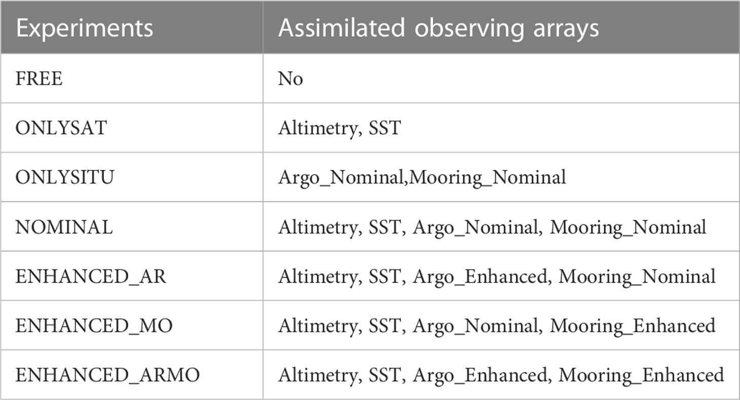
Table 1 Experiments performed in this study. Note that altimetry refers to the assimilation of SSH at the location of observed SLA.

The common synthetic satellite observations consist in sea surface height (SSH) and sea surface temperature (SST) variables (Figure 1); synthetic sea ice concentration is not generated nor assimilated. The SSH data set is built from a constellation of the three nadir satellites Jason-2, Jason-3 and Sentinel-3a. Positions (longitude, latitude, time) are extracted from Copernicus Marine Service Sea Level TAC (Thematic Assembly Center) multi-mission along-track L3 altimeter products. Each satellite provides around 50,000 measurements per date (10-day repeat cycle and 13 orbits per day for Jason-2 and Jason-3; 27-day repeat cycle and 14 orbits per day for Sentinel-3a). The SST data set consists in daily maps obtained from the Copernicus Marine Service ODYSSEA multi-sensor L3S product. This product, consisting in a fusion of SST observations from multiple satellite sensors, daily, over a 0.1° resolution global grid, was used to mask regions without SST observations.

FIGURE 1

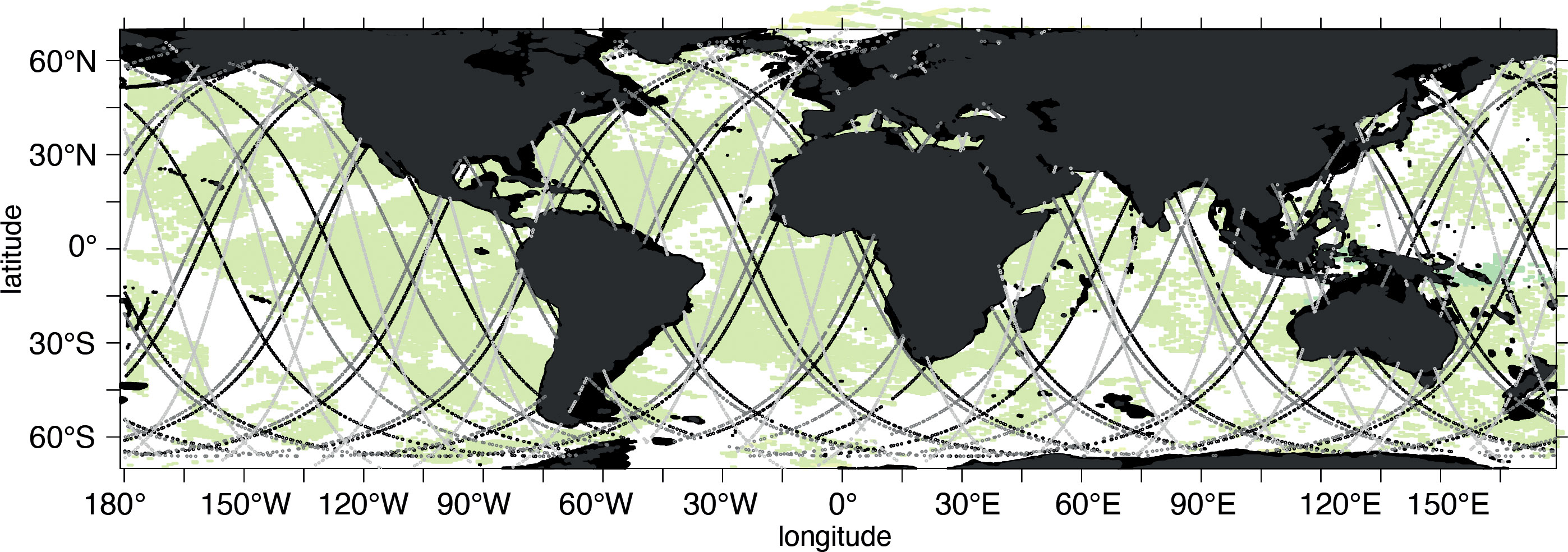
Figure 1 Configurations of synthetic SST (shading) and SSH (curves) observations for a given day. SST maps have been masked out following the ODYSSEA L3S product. SSH sampling corresponds to the orbitals of Jason-2, Jason-3 and Sentinel-3a altimeters.

The synthetic in situ data sets consist of subsurface vertical profiles of temperature and salinity (T/S profiles) from two historical global in situ networks; the Argo global array of profiling floats (www.argo.net) and the Global Tropical Moored Buoy Array (GTMBA, www.pmel.noaa.gov/gtmba). Unlike satellite observations, synthetic in situ observations are built on idealized configurations to ease the interpretation of results. For each of those networks, two different designs are considered representing the current (NOMINAL) and enhanced (ENHANCED) arrays as follows (Figure 2).

● Argo-NOMINAL mimics the standard configuration and corresponds to one Argo float per 3°x3°x10-day square, sampling the 0-2000 m upper-ocean globally. Locations of T/S profiles are randomly distributed in a 3°x3° square, each square being sampled every 10 days. The day of the first 10-day cycle is randomly distributed in the first 10-day window and the space position is different for each 10-day cycle. This T/S configuration counts around 470 profiles per day from 3700 floats, with measurements located at the model vertical levels (including 22 levels within the upper 100 m, with 1-m resolution at the surface and 450-m resolution at the bottom).

● Argo-ENHANCED is based on the latter configuration, with one added float per 3°x3° square in highly energetic regions, i.e, in western boundary currents and in equatorial/tropical regions following international recommendations (Roemmich et al., 2019; Smith et al., 2019). As Argo-NOMINAL, the day of the first 10-day cycle of additional profiles is randomly distributed in the first 10-day window.

● Mooring-NOMINAL uses the position of tropical moorings during the 2020-2021 period (only two TRITON moorings in the western tropical Pacific). Vertical levels of T/S profiles are based on “standard instrumental depths” given by the GTMBA website. Eleven depth levels are located between the surface and 500 m, with 20-m resolution in the upper 150 m. Note that, unlike in the Indian and Atlantic Ocean, there are only temperature profiles in the Pacific.

● Mooring-ENHANCED is mostly characterized by an increased vertical resolution, which follows the recommendations of the tropical community (Foltz et al., 2019; Hermes et al., 2019; Smith et al., 2019), and by a reconfiguration of the Pacific array. Temperature sensors lie at 1 m, every 5 m from 5 to 30 m, every 10 m from 30 to 60 m, and with vertical resolution like present from 60 to 500 m (depending on the longitude in the basin). Salinity sensors are located at 1 m, every 5 m from 5 to 30 m, every 10 m from 30 to 80 m and at 100 m. The strong modification of the spatial distribution of tropical moorings in the Pacific follows the conclusions from the Tropical Pacific Observing System 2020 (Kessler et al., 2021).

FIGURE 2

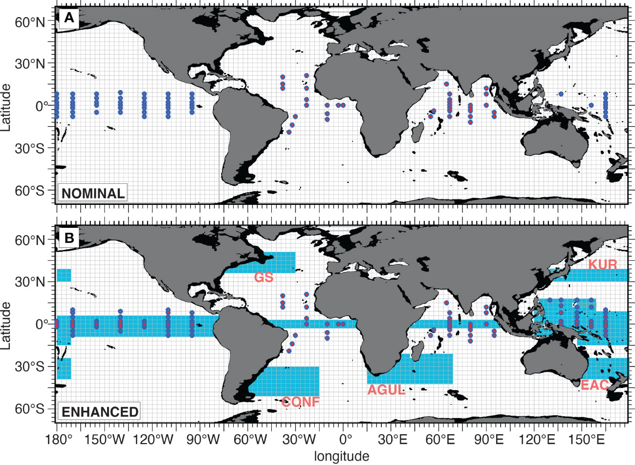
Figure 2 Nominal (A) and enhanced (B) configurations of synthetic temperature and salinity (T/S) profiles for Argo floats (shading) and tropical moorings (dots). Argo sampling corresponds to 1 and 2 floats per 3°x3°x10-day square in yellow and light blue, respectively. Subsurface T/S observations from moorings are indicated by blue (T) and red (S) dots.

To mimic the assimilation procedure of real observations within an operational system, synthetic data sets must deviate from the simulation in which they are assimilated, but also from the Nature Run realization: errors must be prescribed to the synthetic observations, as in the real system. We follow the methodology of Gasparin et al. (2019) to add errors of the synthetic satellites and in situ observations. It should be first noted that synthetic observations are generated from the Nature Run daily mean fields, which are at a higher horizontal resolution (at 1/12° resolution) than the experimental analysis system (at ¼° resolution) in order to consider variability in the synthetic observations associated with processes resolved in the 1/12° system, but not in the ¼° system. Observation error must include a representation error and an instrumental error. The representation error is generated to mimic unresolved or poorly resolved small-scale processes by the data assimilation scheme used in the OSSEs (e.g., internal waves), with horizontally and vertically correlated errors. For that, a time-shifting technique, usually used by the atmosphere community (e.g., Huang and Wang, 2018), generates weekly variability by randomly shifting the Nature Run fields by ± 3 days (following a uniform distribution, either 3 days before or 3 days after the given date). Finally, an instrumental error is added to each observation as an uncorrelated error following a Gaussian distribution with the standard deviation given by the instrumental accuracy (0.35°C for SST; 3 cm for SSH; 0.01°C/0.01 for Argo T/S profiles; and 0.02°C/0.02 for Mooring T/S profiles; Cabanes et al., 2013). We call “synthetic observation error” the sum (in variance) of these different of additional errors.

2.3 Experiments calibration

2.3.1 Synthetic observation error

As the reliability of OSSEs to correctly provide impact assessment partly lies in defining appropriate errors associated to synthetic observations, the representation error is first evaluated for the 100-m temperature and 10-m salinity by computing Root-Mean-Square difference between the original Nature Run fields and the 3-day shifted Nature Run fields. This representation error is of the order of O(0.2°C) for 100-m temperature and O(0.05) for 10-m salinity, with high variability in western boundary regions, tropics, and the Southern Ocean (Supplementary Figure S1). Both instrumental error and error due to the small-scale variability embedded in the 1/12° Nature Run not represented by the ¼° OSSE grid, are negligible in comparison to representation error (not shown), in agreement with Gasparin et al. (2019). The consistency of the synthetic observation errors is measured by comparing the synthetic observation error with observation error prescribed in the data assimilation system. A similar comparison is then carried out at three mooring locations in the equatorial Pacific (Supplementary Figure S2). Profiles of the amplitude of the representation error show a maximum at the thermocline level (~0.8°C), which is slightly higher than the observation error variance specified in the operational system (~0.5-0.8°C). These error estimates are also well-compared with the amplitude of the high-frequency variability of temperature (periods shorter than the 7-day assimilation window) based on the 10-min mooring time series. This indicates that the amplitude of the synthetic observation error, representing high-frequency variability, is thus realistic and in agreement with observation error variance specified in the operational system.

2.3.2 Residual error

To evaluate the good calibration of the experimental analysis system (see Halliwell et al., 2014), it is important to verify that the distance between the assimilated and non-assimilated runs is similar to that of the GLORYS12 reanalysis. If the NOMINAL observing system is comparable with the current observing system, the distance between NOMINAL and FREE experiments must be similar to that of GLORYS12 and its free version FREEGLORYS12. In Figures 3A, B the 100-m temperature and 10-m salinity RMS difference between NOMINAL and FREE experiments, zonally averaged, ranges between 1.0 and 1.5°C for temperature and 0.25 to 0.75 for salinity, and is similar to the RMS difference computed from the difference between GLORYS12 and FREEGLORYS12 (slightly higher for temperature). In addition, the distance of NOMINAL from the synthetic observations is compared with the distance of GLORYS12 from real observations at a mooring point in the equatorial Atlantic (Figures 3C, D). The similar shape of the profiles also provides a good confidence of the good calibration of the experimental analysis system and therefore a realistic behavior of OSSEs.

FIGURE 3

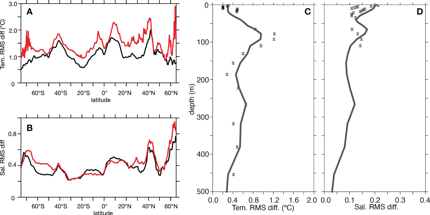
Figure 3 (A, B) 100-m temperature and 10-m salinity RMS difference, zonally averaged, between the free and assimilated simulations for the OSSE system (FREE and NOMINAL; black) and the reanalysis system (FREEGLORYS12 and GLORYS12; red). (C, D) Temperature and salinity RMS residuals (difference of OSSEs fields from the Nature Run fields) at 23°W, 0° (Atlantic) from the OSSE system (distance between NOMINAL and synthetic observations) and the GLORYS12 reanalysis.

3 Spatial and temporal scales constrained by ocean observations

Given the sparse distribution of ocean observations, usual metrics in operational centers are mostly based on box-averaged statistics (Hernandez et al., 2009), making difficult to separate analysis skills according to spatial and temporal scales. To evaluate the ability of ocean observations to constrain ocean state estimates in the experimental analysis system, time series of sea surface steric height (relative to the bottom and referred in the following as steric height) from the FREE experiment, is first analyzed with separation of spatial and temporal scales. To ease the understanding of this global study, we choose to decompose signals and associated errors into three different space and time scales, although more complex techniques could have been used such as Ensemble Empirical Mode Decomposition (EEMD). Temporal and spatial scales shorter than 20 days and 100 km, respectively, are referred to as “small-scale variability”. Small-scale variability, not resolved by the 7-day assimilation window and the ¼° horizontal grid of the eddy-permitting model, is isolated by applying a 1°x1°x20-day high-pass filter on the gridded fields. Note that this small-scale variability includes part of the mesoscale activity which cannot be resolved (and constrained by observations) given the experimental system (Cipollone et al., 2017; Yu et al., 2022). Using a similar filter than Roemmich and Gilson (2009), large-scale signals are obtained by applying a 9°x9°x100-day low-pass running mean filter to represent “large-scale variability”. Finally, the difference between the 9°x9°x100-day and 1°x1°x20-day smoothed time series is referred to “intermediate-scale variability” to define processes such as mesoscale eddies (which can extent to 500-1000 km; Storer et al., 2022) and intraseasonal waves, with temporal and spatial scales of 20-100 days and around 100-1000 km, respectively. In addition, the term “residual error” refers to statistics based on the difference of OSSEs fields from the Nature Run fields. Note that our results do not depend sensitively on specific choice of scales separation, since other choices (e.g., 8°x8°x80-day, 10°x10°x100-day) yield similar results (not shown).

3.1 Variability amplitude for various scales

Figure 4A first shows the total variability of steric height from the FREE experiment. High variability regions are clearly identified in western boundary regions and in the Southern Ocean, with amplitude reaching more than 12 cm. These regions are characterized by instabilities of the strong mean flow generating meanders and eddies (Ducet and Le Traon, 2001). Moderate variability regions are seen in the tropical Indian Ocean and Pacific Ocean. Low variability regions are in the center of oceanic gyres. The standard deviation of steric height was then zonally averaged to show the latitude dependence of the total variability (Figure 4B), and spatial and temporal filters were applied to isolate the steric height variability at small, intermediate and large scales (Figure 4C). At latitudes of the high and moderate variability regions, intermediate variability represents almost 70% of the variability. At other latitudes, large-scale variability is equal or higher than intermediate variability. Small-scale variability, which is usually dominated by coherent vortices, fronts and filaments, represents a non-negligeable contribution to the total variability.

FIGURE 4

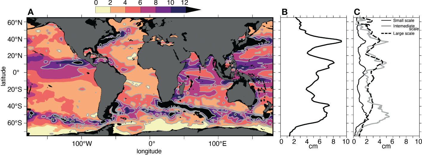
Figure 4 Standard deviation of the daily steric height (SH, cm) from the FREE experiment (A) spatial map, (B, C) zonal-average, black line). For comparison, zonally averaged standard deviation of the daily SH fields of the small scales (black line), intermediate (gray line) and large-scale variability (dashed line) are also shown.

The amplitude of the small-, intermediate and large-scale variability is then compared to the residual error of the FREE experiment, estimated by the RMS difference from the Nature Run fields (Figure 5). The amplitude of the total residual error (including small-, intermediate- and large scales) is quite similar to the total variability of the SH signal, with slightly higher error amplitude at latitudes of high variability regions and slightly lower error amplitude in the tropical band (Figure 5A). Yet, the scale separation demonstrates that the amplitude of the residual error of the FREE experiment is differently distributed over scales than that of the variability (Figures 5B-D). High variability regions of the Northern Hemisphere have similar amplitude at intermediate and large scales, but the FREE residual error is mostly dominated by intermediate scales (mesoscale).

FIGURE 5

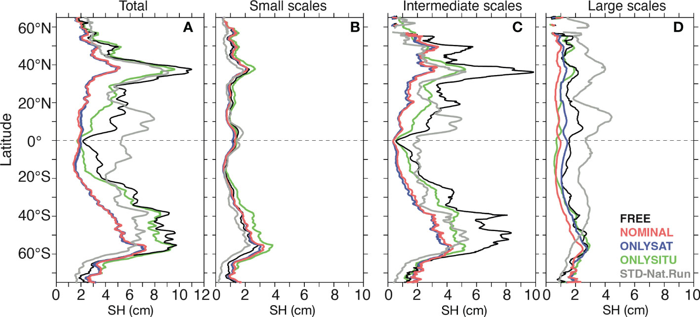
Figure 5 Zonally averaged steric height (SH, cm) RMS difference between the Nature Run and experiments (FREE, NOMINAL, ONLYSAT, ONLYSITU) for the total (A), the small scales (smaller than 1°x1°x20-day, B), mesoscale (between 1°x1°x20-day and 9°x9°x90-day, C) and large variability (larger than 9°x9°x90-day, D). For comparison, the standard deviation of the Nature Run SH, zonally-averaged, is also shown (gray).

Residual errors are usually defined based on the total RMS difference between observations and analysis, without scale separation, and we clearly see the limit of this diagnostic here: it favors the dominant scales of the residual error but does not inform us on the processes that are, or not, constrained by the assimilation. This metric does not either weight the residual error amplitude according to the natural variability. We propose here to define the metric “percent of represented variance”, calculated as one minus the proportion of the residual variance (e.g., the variance of the residual error divided by the signal variance), and to compute it for different scales. We argue it will allow better assessing the impact of the observing system components.

3.2 Impact of the various observing system components

Based on the comparison of several experiments assimilating separately (ONLYSAT, ONLYSITU) and conjointly satellites and in situ data sets (NOMINAL), the aim here is to disentangle the contribution of the satellite versus in situ components in improving the ocean state by separating impacts according to spatial and temporal scales. Note that the data assimilation system uses multi-variate approach meaning that SSH, temperature, salinity corrections are dynamically consistent. ONLYSAT assimilating SSH will provide information on SH, as well as ONLSITU assimilating temperature and salinity (indirectly SH).

3.2.1 Added value of satellites for mesoscale activity

Figure 5C shows the residual errors for steric height at intermediate scales. Even though the magnitude of residual error in ONLYSITU is lower than in FREE, it remains higher than the variability at almost all latitudes. In contrast, an important reduction of the residual error is seen in ONLYSAT, especially at latitudes of western boundary currents where the residual error decreases to 3-4 cm, in comparison to 8-10 cm in FREE. With a residual error at intermediate scales similar to that of ONLYSAT, NOMINAL benefits from satellite observations. This is not a surprise, as this is consistent with the scales of conventional one-dimensional nadir-looking altimeters having the ability to resolve wavelengths down to about 50–150 km depending on the specific satellite and geographic locations (Dufau et al., 2016; Ballarotta et al., 2019).

Sea surface height information provided by altimetry is a depth-integrated quantity and is closely related to steric height. Note that SSH and SH differ by the barotropic component (mass-related component) which is not considered in SH. A question arises on how the information provided by satellites is projected at depth. Some indications are given in Figures 6A, B, showing the globally averaged percentage of the Nature Run represented variance at intermediate scales for each experiment. First, for intermediate scales, the surface layer is better constrained by observations than the deeper layer, both for temperature and salinity, for all experiments. Then, satellite observation impacts (ONLYSAT) are clearly seen in both temperature and salinity variables at intermediate scales on the whole water column. In temperature, ONLYSAT leads to an improvement of 15% of variance at 500 m depth compared to FREE, to 50% at the surface. In salinity, the improvement is more modest: 5% of salinity variance at 500m depth to 30% at the surface. In comparison, the contribution of in situ observations (ONLYSITU) can represent up to half of the improvement seen in ONLYSAT at intermediate scales.

FIGURE 6

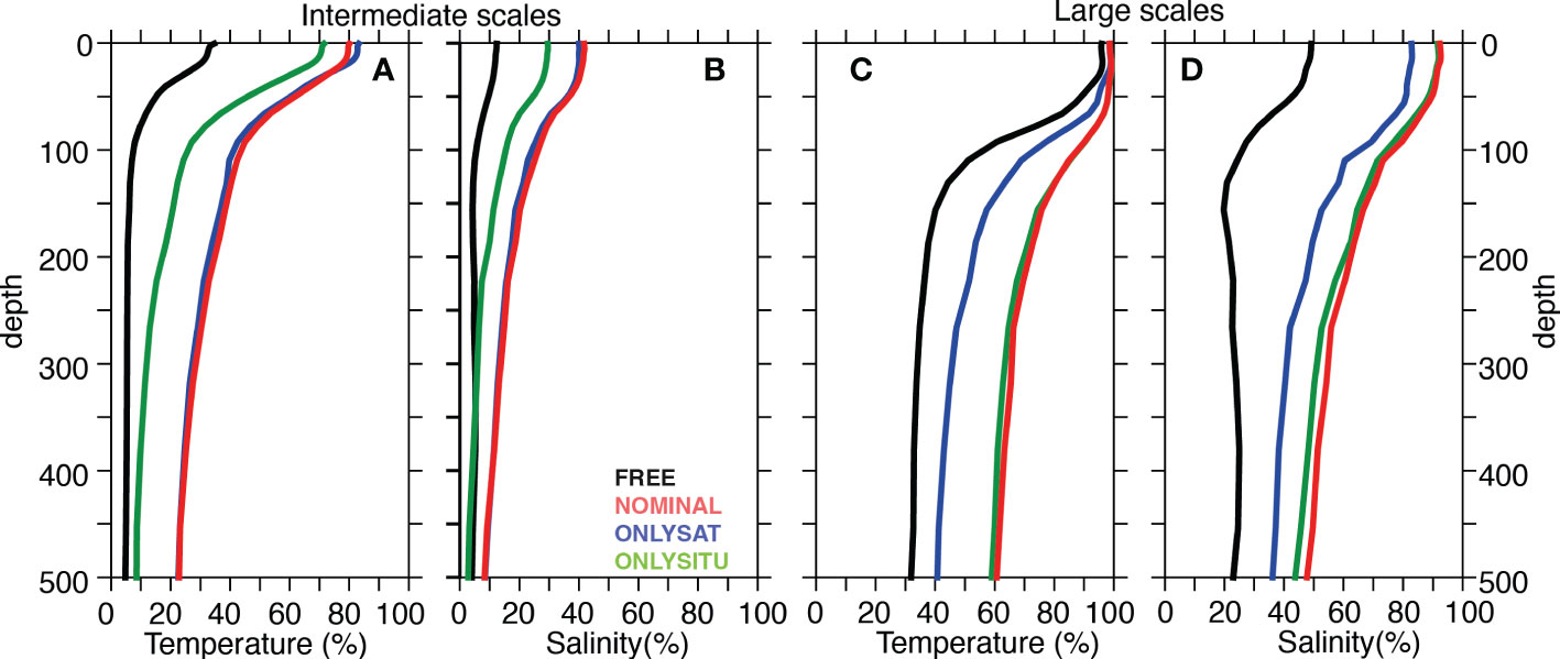
Figure 6 Globally averaged percentage of Nature Run represented variance for subsurface temperature and salinity at intermediate (A, B) and large scales (C, D) from the FREE, NOMINAL, ONLYSAT, ONLYSITU experiments. Timeseries have been filtered with running mean filters (1°x1°x20-day, 9°x9°x90-day) as explained in the text.

3.2.2 Added value of in situ observations for large-scale variability

At larger scales, residual errors in OSSEs are significantly lower than variability for all experiments (Figure 5D), including the unconstrained FREE experiment, likely due to the more predictable large-scale response of the ocean circulation to atmospheric forcing at low frequencies (Wunsch, 1998). Compared to FREE, the reduction of the residual error is more important in ONLYSITU than in ONLYSAT, suggesting that in situ observations provide a unique large-scale information to the analysis (similar residual error between ONLYSITU and NOMINAL). This is consistent with the characteristics of the Argo array which provides a global coverage of the upper ocean on broad spatial scales, O(1000 km), and on time scales of months and longer (Roemmich and Gilson, 2009; Riser et al., 2016). The higher impact of in situ compared to satellites observations is confirmed in Figures 6C, D. In the FREE experiment, the percentage of represented variance of temperature is close to one at the surface and decreases to 30% in depth. In situ observations (ONLYSITU) improves the large-scale thermohaline stratification by increasing the percentage of represented variance by around 30% at depth for temperature, and up to 50% for salinity. In comparison, improvement from satellites observations (ONLYSAT) is lower, demonstrating a clear added value of in situ observations at large scales/low frequency.

The computation of statistics on residual errors by separating spatial and temporal scales highlights the evidence for the complementary role of satellites and in situ observations for constraining ocean analysis, with intermediate scales (mesoscale) mostly constrained by satellites and large scales by in situ observations. However, the reduction of analysis error at mesoscale is not null in ONLYSITU, as at large scales for ONLYSAT experiment, and the residual error reduction in NOMINAL is not directly related to the sum of ONLYSAT and ONLYSITU improvements. Both in situ and satellites observations provide a redundant information with regards to ocean analysis at a given spatial and temporal scale. This can explain the higher impact of in situ observations in ocean analysis when satellites observations are not assimilated (e.g., Zhu et al., 2021).

4 Potential outcomes of in situ observing system enhancements

The next objective of the present work is to evaluate potential outcomes of enhancing the in situ ocean observing system. One of the major evolutions of the in situ observing system recommended by the international community (Oceanobs’19 conference) is to double the number of Argo floats in western boundary currents and in equatorial regions and to enhance the vertical resolution of temperature and salinity measurements in the upper ocean layer on tropical moorings (Foltz et al., 2019; Smith et al., 2019; Hermès et al., 2019). Such evolutions have been evaluated based on three additional experiments (ENHANCED_AR, ENHANCED_MO, ENHANCED_AR_MO; Table 1).

4.1 Doubling Argo in western boundary currents

Western boundary currents are a fundamental element in the ocean circulation system given their impact on weather and climate both locally and remotely, on time scales from days to decades. Yet, it has been recognized that estimates of heat and freshwater contents have still large uncertainties due to insufficient sampling (e.g., Palmer et al., 2019, Todd et al., 2019). With high levels of mesoscale variability, enhancing Argo sampling in western boundary current is expected to reduce noise in tracking the temperature and salinity fields (Roemmich et al., 2019). The impact of doubling the number of Argo floats on constraining oceanic analyses will thus be assessed based on the experiment ENHANCED_AR, in which the number of Argo profiles has been doubled in western boundary current regions. For the assessment, we use integrated quantities as the ocean heat content (OHC) and the ocean freshwater content (OFC). The 0-700m OHC is computed based on the depth-integration of temperature anomaly from the 2016-2017 temporal mean multiplied by the heat capacity (3900 J/kg/°C) and ocean density of reference (1024 kg/m³). Considering that about 3 cm of freshwater are needed to dilute 1 m of seawater by 1 psu, the OFC, expressed in meters, is the depth-integral of salinity anomaly multiplied by -0.03 (Gasparin and Roemmich, 2016).

Figure 7 shows the percentage of the OHC and OFC represented variance of the Nature Run for each experiment, area-averaged in the five main western boundary current regions (see Figure 1). OHC and OFC time series have been previously filtered to separate intermediate to large-scale variability. As expected, large-scale structures are better represented than intermediate scale features, with more than 90% of the OHC variance (Figure 7A) and more than 50% of the OFC variance (Figure 7C) represented by the NOMINAL experiment (in red). In agreement with previous results, in situ observations are generally more efficient than satellites observations in constraining the large-scale OHC and OFC variability (comparing blue and green bars in Figures 7A, C). This is more obvious for OFC. In addition, important differences between ONLYSAT (in blue) and ONLSITU (in green) experiments to represent both intermediate scales OHC and OFC confirm the key role of satellites observations to constrain mesoscale variability (Figures 7B, D). The complementarity of both observing system components is confirmed since the percentage of represented variance is systematically higher in NOMINAL than in ONLYSITU or ONLYSAT, especially in large-scale OFC where NOMINAL percentages of the Nature Run represented variance are 10 to 20% higher than that of ONLYSITU.

FIGURE 7

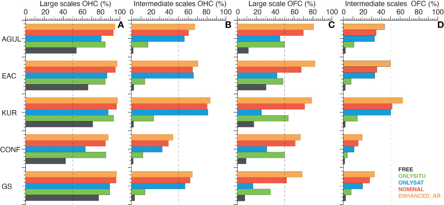
Figure 7 Percentage of the Nature Run represented variance, area-averaged in western boundary current regions, for 0-700 m Ocean Heat (OHC, A, B) and Freshwater Contents (OFC, C, D) at mesoscale and larger scales based on the FREE (black), NOMINAL (red), ONLYSAT (blue), ONLYSITU (green) and ENHANCED_AR (orange) experiments.

The added value of doubling the number of Argo floats is then assessed by comparing NOMINAL with ENHANCED_AR (in orange). Compared to NOMINAL, the slightly increased percentages of represented variance in ENHANCED_AR for both intermediate and large-scale OHC suggest that doubling Argo in western boundary current regions only has a limited impact on OHC. In contrast, substantial gain is seen for salinity (OFC) at both intermediate and large scales with improvements reaching more than 10% (e.g, Agulhas, EAC, Kuroshio regions). These results are qualitatively consistent with the reduction of the RMS error in the Gulf Stream from the multi-system approach of Gasparin et al. (2019).

4.2 Argo doubling and mooring enhancements in tropics

We now focus on the potential impacts of enhanced observing systems in the tropical oceans. Several extensions of the Argo and moored arrays have been proposed, both to help constraining the ocean state via their ingestion in data assimilation systems, and to help understanding critical processes not well sampled (Cravatte et al., 2016). These enhancements consist in a finer vertical resolution in the upper 100 meters, and an enhanced meridional resolution, with Argo doubling and more sensors on moorings in the upper ocean. The comparison, based on experiments in which Argo and moorings arrays have been enhanced separately or together (ENHANCED_AR, ENHANCED_MO and ENHENCED_AR_MO), aims at determining the relative and combined impacts of in situ enhancements. Results are shown for the Pacific Ocean, but conclusions can be extended to other tropical basins.

Figures 8A-D indicates the percentage of Nature Run represented variance for the 0-100m temperature and salinity at intermediate and large scales for NOMINAL and ENHANCED_AR_MO experiments, zonally averaged in the tropical Pacific. While NOMINAL can capture more than 70% of the Nature Run variance for temperature and salinity at both intermediate and large scales, only slight improvements are seen in ENHANCED_AR_MO (less than 5% higher than NOMINAL, area-averaged in the tropical Pacific). However, zonal averages mask a more complex behavior of the data assimilation system. In Figures 8E, F the difference of the percentage of the Nature Run represented variance at intermediate scales between ENHANCED_AR_MO and NOMINAL experiments for the 0-100 m layer indicates that in situ enhancements generally reduce residuals errors of temperature and salinity (Figures 8A, B), but improvement can reach 35% of the Nature Run variance of salinity in the western Pacific, while degradations are seen in some areas (higher residuals in ENHANCED_AR_MO than in NOMINAL).

FIGURE 8

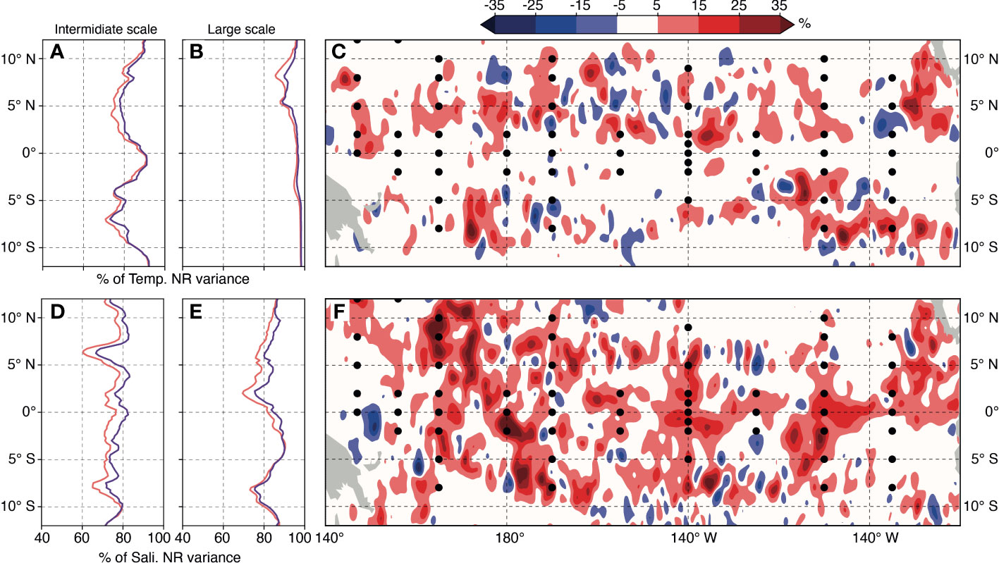
Figure 8 Zonally averaged percentage of Nature Run represented variance of NOMINAL (red) and ENHANCED_AR_MO (purple) experiments for the 0-100m temperature (A, B) and salinity (D, E) at intermediate and large scales. (C, F) ENHANCED_AR_MO-minus-NOMINAL difference of percentage of Nature Run represented variance at intermediate scales for the 0-100m (C) temperature and (F) salinity.

The higher improvement in salinity results from the increased number of subsurface salinity measurements in ENHANCED_AR_MO (no salinity at mooring locations in NOMINAL), and since salinity is less constrained by altimetry as sea level variations are dominated by the thermosteric component (Storto et al., 2017). The degradation at some locations in ENHANCED_AR_MO might be due to several reasons. First, the number of temperature observations on moorings is decreased off-equator in ENHANCED_AR_MO compared to NOMINAL (See Figure 2). The percentage of variance, based on the ratio of error variance and signal variance, computed on the 2016-2017 period, underestimates in situ enhancement impacts due to the strong variability associated with the 2015-2016 El Nino. It is also noteworthy that data assimilation systems are built on subtle balances and conservation laws, data assimilation can also result in small degradations (e.g., Waters et al., 2017).

It is now possible to separate the effects of each component of the in situ observing system by comparing the percentage of Nature Run represented variance for temperature and salinity at intermediate and large scales, zonally averaged in the tropical Pacific, for ENHANCED_AR and ENHANCED_MO experiments (Figure 9). Interesting features are seen. First, temperature is not significantly improved at both intermediate and large scales, except off-equator where doubling Argo (ENHANCED_AR) increases the percentage of represented variance of 5% on average. Note that the percentage of variance is close to 90% in the equatorial band. The representation of the 0-100m salinity at intermediate scales is improved in both ENHANCED_AR and ENHANCED_MO. While doubling Argo benefits to all latitudes, mooring enhancements only provide a better estimate in the 4°S-4°N band. Such equator/off-equator differences are due to the fixed-point characteristics of moorings with a smaller number of salinity measurements in addition to shorter scales dynamics off-equator. At large scales, salinity benefits similarly from both Argo and moorings enhancements.

FIGURE 9

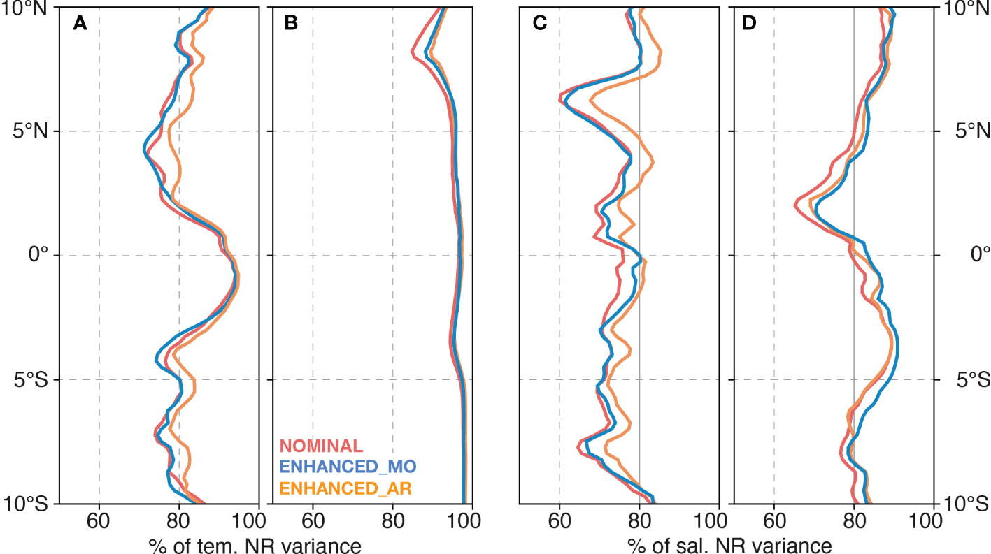
Figure 9 Percentage of Nature Run (NR) temperature (A, B) and salinity (C, D) represented variance at intermediate (A, C) and large (B, D) scales for NOMINAL (in red), ENHANCED_MO (blue), ENHANCED_AR (orange) experiments, zonally averaged in the tropical Pacific.

Similar diagnostics are applied to integrated quantities such as mixed layer depth (MLD) and barrier layer thickness (BLT) computed following the definition of de Boyer Montégut et al. (2004). Figure 10 shows the percentage of represented Nature Run variance at intermediate scales, zonally averaged in the western Pacific between 135°E and 155°E, for NOMINAL and the ENHANCEDs experiments. Different behaviors are seen. First, doubling Argo (ENHANCED_AR, yellow) systematically provides a better estimate than NOMINAL (red), while benefits from moorings do not occur at all latitudes. Even if ENHANCED_AR_MO often provides the best estimates, suggesting that both Argo and mooring data assimilation are complementary (south of 2°N), dedicated work is still necessary to make a better use of mooring observations (e.g., at 3°N).

FIGURE 10

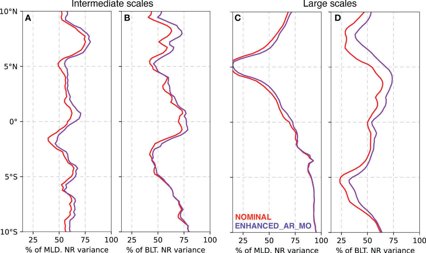
Figure 10 Percentage of Nature Run represented variance of Mixed Layer Depth and Barrier Layer Thickness at intermediate scales (A, B) and large scales (C, D) for the NOMINAL and ENHANCED_AR_MO experiments, zonally averaged in the western Paci!c (140E-180°E).

Thus, in situ enhancements slightly improve the representation of temperature and salinity fields at both intermediate and large scales, with a strong regional dependency. A higher impact is seen in salinity (not directly constrained by altimetry), at both intermediate and large scales. However, as data assimilation techniques favor local impacts, moorings generally provide a highly accurate representation near the mooring points (at the thermocline level, Figure 11), while Argo gives a more uniformly accurate estimate across the basin (Figure 10A). The strong complementarity between these two components is seen since both type of information benefit to the data assimilation system (Figure 11C), in agreement with previous studies (e.g., Gasparin et al., 2015; Zhu et al., 2021). It is important to mention that positive impacts of additional observations also result in some degradation (below 150m in Figure 11B). Further investigations are thus required to optimize the use of ocean observations and avoid spurious effects of data assimilation.

FIGURE 11

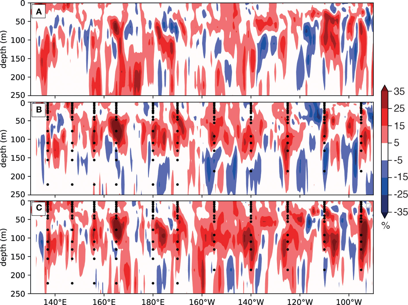
Figure 11 Difference of percentage of Nature Run (NR) salinity represented variance at intermediate scales from the NOMINAL experiment for (A) ENHANCED_AR, (B) ENHANCED_MO and (C) ENHANCED_AR_MO experiments along the equatorial Pacific. Red colors represent improvement of enhanced experiments compared to NOMINAL.

5 Discussion and conclusion

Based on a series of observing system simulation experiments (OSSE), a detailed description of the impacts of various ocean observations (from satellites and in situ networks) assimilated in a global data assimilation system is presented here. One of the important novelties here is the decomposition of the signals (both residual errors and percentage of represented variance) into specific temporal and spatial scales (i.e., small scales, intermediate scales and large scales). This allows a better understanding of the relative contributions of the observing system components in constraining various processes.

In general, mesoscale processes dominate residual errors in simulations with no data assimilation, especially in western boundary currents, while they are equivalent to large-scale residual errors in mid-latitude and low-latitude regions. Our experiments assimilating conjointly satellites and in situ data sets demonstrate the ability of an analysis system to represent 40-80% of the temperature variance at intermediate scales (20-30% for salinity), and more than 80% of the variance for large-scale variability. An important complementarity of satellites and in situ observations is shown; satellites information, mostly through altimetric data, strongly constrain mesoscale variability, while in situ data, mostly through Argo floats, provide a large-scale information. Each observing system component provides a substantial added value for ocean state estimates depending on the selected spatial and temporal scales. In addition to depth-integrated quantities, such as steric height, the added value of the observing system is clearly seen for subsurface temperature and salinity.

In addition to the evaluation of the current observing system design, our numerical experimental system also assessed the expected impact of future enhancements in observing systems, as recommended by GOOS. One of the main recommended enhancements is the doubling of the number of Argo floats in western boundary currents regions. It is demonstrated that the representation of the ocean freshwater content in these regions would be significantly improved, at both intermediate (mesoscale) and larger scales, whereas the representation of ocean heat content would be mostly improved at mesoscale. Enhancements of moorings observations are mostly through additional temperature and salinity sensors in the tropical Pacific (and a modification of the mooring locations in the tropical Pacific), and an increase in the vertical resolution in the surface layer in the Indian and Atlantic basins. In addition to substantial improvements at large scales, impacts of these enhancements are mostly seen locally as also seen in several studies (e.g., Gasparin et al., 2019; Zhu et al., 2021). Further developments of data assimilation systems might be needed to make a better use of these observations in models.

Unlike many other data assimilation systems, the benefits of in situ ocean observations are estimated here as a complementary information to satellite data sets (Fujii et al., 2019). The number of experiments, including simulations that assimilate observing system components separately, is a central point of this study and demonstrates the complexity of impact studies in a multivariate system. As expected, benefits of in situ observations are lower in the context of the integrated observing system. One limitation of this study is that results are obtained with a particular operational system. Efforts have been made to extract important messages that can likely be applied to other ocean analysis systems. However, it is noteworthy that observations impacts can be dependent on the data assimilation techniques and settings, and that similar experiments should be made for other systems to complement our results. More advanced techniques might hopefully increase the gain of a specific observing system component.

Finally, it is worth pointing out that the impact of ocean observations on analyses is addressed here only from the assimilation perspective. Ocean observations have multiple other benefits: they are key at the different steps of the development and qualification of an analysis system: they foster forecasting system advancement through a better understanding of the climate system; they allow validation and verification. All these indirect contributions are also very important for the analysis accuracy, albeit less visible.

Data availability statement

The raw data supporting the conclusions of this article will be made available by the authors, without undue reservation.

Author contributions

FG designed and wrote the manuscript. FG and J-ML generated synthetic observations, setted up the experimental system and performed experiments. FG conducted most of the analyses, with substantial contributions from J-ML, SC, GR and ER. Lastly, PL and BR helped in reading, editing figures and commenting on the paper. All authors contributed to the article and approved the submitted version.

Funding

This project has received funding from the European Union’s Horizon 2020 research and innovation program under grant agreement No.892626 (EUROSEA).

Acknowlegments

This study was conducted using Copernicus Marine Service Products. This paper used data collected and made freely available by programs that constitute the Global Ocean Observing System and the national programs that contribute to it (http://www.ioc-goos.org/), i.e., the Argo data collected and made freely available by the International Argo Project and the national programs that contribute to it (http://argo.jcommops.org), the TAO-PIRATA-RAMA (PMEL-NOAA).

Conflict of interest

The authors declare that the research was conducted in the absence of any commercial or financial relationships that could be construed as a potential conflict of interest.

Publisher’s note

All claims expressed in this article are solely those of the authors and do not necessarily represent those of their affiliated organizations, or those of the publisher, the editors and the reviewers. Any product that may be evaluated in this article, or claim that may be made by its manufacturer, is not guaranteed or endorsed by the publisher.

Supplementary material

The Supplementary Material for this article can be found online at: https://www.frontiersin.org/articles/10.3389/fmars.2023.1021650/full#supplementary-material

Supplementary Figure 1 | Amplitude of errors (both representation and instrumental) associated to synthetic observations for 100-m temperature and 10-m salinity: (A, C) spatial maps, (B, D) zonally averaged (black line). As a comparison, zonally averaged prescribed error in the operational system is also shown in red line. Amplitude of synthetic observation errors (both representation and instrumental errors) in synthetic observations for 100-m temperature: (A) spatial maps, (B) zonally averaged (black line) and for 10-m salinity (C) spatial maps, (B) zonally averaged (black line). As a comparison, zonally averaged prescribed error in the operational system is also shown in red line in (B) and (D).

Supplementary Figure 2 | Amplitude of errors in synthetic temperature observations at three moorings locations in the equatorial Pacific (165°E, 140°W, 110°W). For comparison to the error estimate (black lines), prescribed errors in the operational system (red lines) and high-frequency variability from moorings (<7 days; blue crosses) are shown.

References

Aydogdu A., Pinardi N., Pistoi J., Martinelli M., Belardinelli A., Sparnocchia S. (2016). Assimilation experiments for the fishery observing system in the Adriatic Sea. J. Mar. Syst. 162, 126–136. doi: 10.1016/j.jmarsys.2016.03.002

CrossRef Full Text | Google Scholar

Ballarotta M., Ubelmann C., Pujol M.-I., Taburet G., Legeais J.-F., Faugere Y., et al. (2019). On the resolution of ocean altimetry maps. Ocean Sci. 156. doi: 10.5194/os-2018-156

CrossRef Full Text | Google Scholar

Balmaseda M., Anderson D. (2009). Impact of initialization strategies and observations on seasonal forecast skill. Geophys. Res. Lett. 36 (1), L01701. doi: 10.1029/2008GL035561

CrossRef Full Text | Google Scholar

Balmaseda M., Anderson D., Vidard A. (2007). Impact of argo on analyses of the global ocean. Geophysical Res. Lett. 34 (16), L16605. doi: 10.1029/2007GL030452

CrossRef Full Text | Google Scholar

Balmaseda M. A., Trenberth K. E., Källén E. (2013). Distinctive climate signals in reanalysis of global ocean heat content. Geophysical Res. Lett. 40 (9), 1754–1759. doi: 10.1002/grl.50382

CrossRef Full Text | Google Scholar

Bell M. J., Schiller A., Pierre-Yves Le T., Smith N. R., Dombrowsky E., Wilmer-Becker K. (2015). An introduction to GODAE OceanView. J. Of Operational Oceanography 8, S2–S11. doi: 10.1080/1755876X.2015.1022041

CrossRef Full Text | Google Scholar

Benkiran M., Greiner E. (2008). Impact of the incremental analysis updates on a real-time system of the north Atlantic ocean. J. Atmos. Ocean. Technol. 25, 2055–2073. doi: 10.1175/2008JTECHO537.1

CrossRef Full Text | Google Scholar

Benkiran M., Ruggiero G., Greiner E., Le Traon P.-Y., Rémy E., Lellouche J. M., et al. (2021). Assessing the impact of the assimilation of SWOT observations in a global high-resolution analysis and forecasting system part 1: Methods. Front. Mar. Sci. 8. doi: 10.3389/fmars.2021.691955

CrossRef Full Text | Google Scholar

Bloom S. C., Takacs L. L., Da Silva A. M., Ledvina D. (1996). Data assimilation using incremental analysis updates. Mon. Weather Rev. 124, 1256–1271. doi: 10.1175/1520-0493(1996)124<1256:DAUIAU>2.0.CO;2

CrossRef Full Text | Google Scholar

Brasseur P., Verron J. (2006). The SEEK filter method for data assimilation in oceanography: a synthesis. Ocean Dyn. 56, 650–661. doi: 10.1007/s10236-006-0080-3

CrossRef Full Text | Google Scholar

Brodeau L., Barnier B., Gulev S. K., Woods C. (2017). Climatologically significant effects of some approximations in the bulk parameterizations of turbulent air–sea fluxes. J. Phys. Oceanogr. 47, 5–28. doi: 10.1175/jpo-d-16-0169.1

CrossRef Full Text | Google Scholar

Cabanes C., Grouazel A., von Schuckmann K., Hamon M., Turpin V., Coatanoan C., et al. (2013). The CORA dataset: validation and diagnostics of insitu ocean temperature and salinity measurements. Ocean Sci. 9, 1–18. doi: 10.5194/os-9-1-2013

CrossRef Full Text | Google Scholar

Cipollone A., Masina S., Storto A., Iovino D. (2017). Benchmarking the mesoscale variability in global ocean eddy-permitting numerical systems. Ocean Dynamics 67 (10), 1313–1333. doi: 10.1007/s10236-017-1089-5

CrossRef Full Text | Google Scholar

Cravatte S., Kessler W. S., Smith N., Wijffels S. E., Yu L., Contributing Authors (2016). Executive Summary. First report of TPOS 2020 (Salisbury: TPOS), GOOS-215, pp. i-xii. Available online at http://tpos2020.org/first-report/.

Google Scholar

Cummings J., Bertino L., Brasseur P., Fukumori I., Kamachi M., Martin M. J., et al. (2009). Ocean data assimilation systems for GODAE. Oceanography 22 (3), 96–109. doi: 10.5670/oceanog.2009.69

CrossRef Full Text | Google Scholar

de Boyer Montégut C., Madec G., Fischer A. S., Lazar A., Iudicone D. (2004). Mixed layer depth over the global ocean: an examination of profile data and a profile-based climatology. J. Geophys. Res. 109, C12003. doi: 10.1029/2004JC002378

CrossRef Full Text | Google Scholar

Dee D. P., Uppala S. M., Simmons A. J., Berrisford P., Poli P., Kobayashi S., et al. (2011). The ERAInterim reanalysis: configuration and performance of the data assimilation system. Q. J. R. Meteorol. Soc 137, 553–597. doi: 10.1002/qj.828

CrossRef Full Text | Google Scholar

Ducet N., Le Traon P.-Y. (2001). A comparison of surface eddy kinetic energy and reynolds stresses in the gulf stream and the kuroshio current systems from merged TOPEX/Poseidon and ERS-1/2 altimetric data. J. Geophys. Res. 106, 16603–16622. doi: 10.1029/2000JC000205

CrossRef Full Text | Google Scholar

Dufau C., Orsztynowicz M., Dibarboure G., Morrow R., Le Traon P. Y. (2016). Mesoscale resolution capability of altimetry: present & future. J. Geophys. Res. Oceans 121, 4910–4927. doi: 10.1002/2015JC010904

CrossRef Full Text | Google Scholar

Foltz G. R., Brandt P., Richter I., Rodríguez-Fonseca B., Hernandez F., Dengler M., et al. (2019). The tropical atlantic observing system. Front. Mar. Sci. 6. doi: 10.3389/fmars.2019.00206

CrossRef Full Text | Google Scholar

Fu L. L., Christensen E. J., Yamarone C. A. Jr., Lefebvre M., Menard Y., Dorrer M., et al. (1994). TOPEX/POSEIDON mission overview. J. Geophysical Research: Oceans 99 (C12), 24369–24381. doi: 10.1029/94JC01761

CrossRef Full Text | Google Scholar

Fujii Y., Ogawa K., Brassington G. B., Ando K., Yasuda T., Kuragano T. (2015). Evaluating the impacts of the tropical pacific observing system on the ocean analysis fields in the global ocean data assimilation system for operational seasonal forecasts in JMA. J. Oper. Oceanogr. 8, 25–39. doi: 10.1080/1755876X.2015.1014640

CrossRef Full Text | Google Scholar

Fujii Y., Rémy E., Zuo H., Oke P., Halliwell G., Gasparin F., et al. (2019). Observing system evaluation based on ocean data assimilation and prediction systems: On-going challenges and a future vision for designing and supporting ocean observational networks. Front. Mar. Sci. 6, 417. doi: 10.3389/fmars.2019.00417

CrossRef Full Text | Google Scholar

Gasparin F., Guinehut S., Mao C., Mirouze I., Rémy E., King R. R., et al. (2019). Requirements for an integrated in situ Atlantic ocean observing system from coordinated observing system simulation experiments. Front. Mar. Sci. 6, 83. doi: 10.3389/fmars.2019.00083

CrossRef Full Text | Google Scholar

Gasparin F., Hamon M., Rémy E., Le Traon P. Y. (2020). How deep argo will improve the deep ocean in an ocean reanalysis. J. Climate 33 (1), 77–94. doi: 10.1175/JCLI-D-19-0208.1

CrossRef Full Text | Google Scholar

Gasparin F., Roemmich D. (2016). The strong freshwater anomaly during the onset of the 2015/2016 El niño. Geophysical Res. Lett. 43 (12), 6452–6460. doi: 10.1002/2016GL069542

CrossRef Full Text | Google Scholar

Gasparin F., Roemmich D., Gilson J., Cornuelle B. (2015). Assessment of the upper-ocean observing system in the equatorial pacific: the role of argo in resolving intraseasonal to interannual variability. J. Atmos. Oceanic. Technol. 32, 1668–1688. doi: 10.1175/jtech-d-14-00218.1

CrossRef Full Text | Google Scholar

Good S. A., Martin M. J., Rayner N. A. (2013). EN4: quality controlled ocean temperature and salinity profiles and monthly objective analyses with uncertainty estimates. J. Geophys. Res. 118, 6704–6716. doi: 10.1002/2013JC009067

CrossRef Full Text | Google Scholar

Halliwell G. R., Srinivasan A., Kourafalou V., Yang H., Willey D., Le Hénaff M., et al. (2014). Rigorous evaluation of a fraternal twin ocean OSSE system for the open gulf of Mexico. J. Atmospheric Oceanic Technol. 31 (1), 105–130. doi: 10.1175/JTECH-D-13-00011.1

CrossRef Full Text | Google Scholar

Hermes J. C., Masumoto Y., Beal L. M., Roxy M. K., Vialard J., Andres M., et al. (2019). A sustained ocean observing system in the Indian ocean for climate related scientific knowledge and societal needs. Front. Mar. Sci. 6. doi: 10.3389/fmars.2019.00355

CrossRef Full Text | Google Scholar

Hernandez F., Bertino L., Brassington G., Chassignet E., Cummings J., Davidson F., et al. (2009). Validation and intercomparison studies within GODAE. Oceanography 22 (3), 128–143. doi: 10.5670/oceanog.2009.71

CrossRef Full Text | Google Scholar

Huang B., Wang X. (2018). On the use of cost-effective valid-time-shifting (VTS) method to increase ensemble size in the GFS hybrid 4DEnVar system. Mon. Weather Rev. 146, 2973–2998. doi: 10.1175/MWR-D-18-0009.1

CrossRef Full Text | Google Scholar

Jones E. M., Oke P. R., Rizwi F., Murray L. (2012). Assimilation of glider and mooring data into a coastal ocean model. Ocean Model. 47, 1–13. doi: 10.1016/j.ocemod.2011.12.009

CrossRef Full Text | Google Scholar

Kessler W. S., Cravatte S., Lead Authors, 2021. “GOOS-268,” in Final report of TPOS 2020, vol. 83. . Available at: https://tropicalpacific.org/tpos2020-project-archive/reports/.

Google Scholar

Lellouche J. M., Greiner E., Bourdallé-Badie R., Garric G., Melet A., Drévillon M., et al. (2021). The Copernicus global 1/12 oceanic and sea ice GLORYS12 reanalysis. Front. Earth Sci. 9, 698876. doi: 10.3389/feart.2021.698876

CrossRef Full Text | Google Scholar

Lellouche J.-M., Greiner E., Le Galloudec O., Garric G., Regnier C., Drevillon M., et al. (2018). Recent updates to the Copernicus marine service global ocean monitoring and forecasting real-time 1/12° high-resolution system. Ocean Sci. 14, 1093–1126. doi: 10.5194/os-14-1093-2018

CrossRef Full Text | Google Scholar

Lellouche J.-M., Le Galloudec O., Drévillon M., Régnier C., Greiner E., Garric G., et al. (2013). Evaluation of global monitoring and forecasting systems at Mercator océan. Ocean Sci. 9, 57–81. doi: 10.5194/os-9-57-2013

CrossRef Full Text | Google Scholar

Le Traon P. Y., Reppucci A., Alvarez Fanjul E., Aouf L., Behrens A., Belmonte M., et al. (2019). From observation to information and users: The Copernicus marine service perspective. Front. Mar. Sci. 6, 234. doi: 10.3389/fmars.2019.00234

CrossRef Full Text | Google Scholar

Levin J., Arango H. G., Laughlin B., Hunter E., Wilkin J., Moore A. M. (2021). Observation impacts on the mid-Atlantic bight front and cross-shelf transport in 4D-var ocean state estimates: Part II–the pioneer array. Ocean Model. 157, 101731. doi: 10.1016/j.ocemod.2020.101731

CrossRef Full Text | Google Scholar

Madec G., The NEMO Team. (2008). NEMO ocean engine, version 3.0. Note du Pôle de modélisation de l’Institut Pierre-Simon Laplace, 27. Paris: Institut Pierre-Simon Laplace (IPSL), pp. 217. Available at: https://epic.awi.de/id/eprint/39698/1/NEMO_book_v6039.pdf

Google Scholar

Madec G., Bourdallé-Badie R., Bouttier P.-A., Bricaud C., Bruciaferri D., Calvert D., et al. (2017). NEMO ocean engine Paris, France: notes Du pôle de modélisation de l’institut Pierre-simon Laplace (IPSL). doi: 10.5281/zenodo.1472492

CrossRef Full Text | Google Scholar

Madec G., Imbard M. (1996). A global ocean mesh to overcome the north pole singularity. Clim. Dynam. 12, 381–388. doi: 10.1007/BF00211684

CrossRef Full Text | Google Scholar

McPhaden M. J., Busalacchi A. J., Cheney R., Donguy J.-R., Gage K. S., Halpern D. (1998). The tropical ocean-global atmosphere observing system: A decade of progress. J. Geophys. Res. 103, 14169–14240. doi: 10.1029/97JC02906

CrossRef Full Text | Google Scholar

Moltmann T., Turton J., Zhang H. M., Nolan G., Gouldman C., Griesbauer L., et al. (2019). A global ocean observing system (GOOS), delivered through enhanced collaboration across regions, communities, and new technologies. Front. Mar. Sci. 6, 291. doi: 10.3389/fmars.2019.00291

CrossRef Full Text | Google Scholar

Moore A. M., Martin M. J., Akella S., Arango H. G., Balmaseda M., Bertino L., et al. (2019). Synthesis of ocean observations using data assimilation for operational, real-time and reanalysis systems: A more complete picture of the state of the ocean. Front. Mar. Sci. 6, 90. doi: 10.3389/fmars.2019.00090

CrossRef Full Text | Google Scholar

Palmer M. D., Durack P., Chidichimo M. P., Church J., Cravatte S. E., Hill K. L., et al. (2019). Adequacy of the ocean observation system for quantifying regional heat and freshwater storage and change. Front. Mar. Sci. 6. doi: 10.3389/fmars.2019.00416

CrossRef Full Text | Google Scholar

Riser S. C., Freeland H. J., Roemmich D., Wijffels S., Troisi A., Belbeoch M., et al. (2016). Fifteen years of ocean observations with the global argo array. Nat. Clim. Change 6, 145–153. doi: 10.1038/nclimate2872

CrossRef Full Text | Google Scholar

Rodi W. (1987). Examples of calculation methods for flow andmixing in stratified fluids. J. Geophys. Res. 92, 5305–5328. doi: 10.1029/jc092ic05p05305

CrossRef Full Text | Google Scholar

Roemmich D., Alford M. H., Claustre H., Johnson K., King B., Moum J., et al. (2019). On the future of argo: a global, full-depth, multi-disciplinary array. Front. Mar. Sci. 6. doi: 10.3389/fmars.2019.00439

CrossRef Full Text | Google Scholar

Roemmich D., Gilson J. (2009). The 2004–2008 mean and annual cycle of temperature, salinity, and steric height in the global ocean from the argo program. Prog. Oceanogr. 82, 81–100. doi: 10.1016/j.pocean.2009.03.004

CrossRef Full Text | Google Scholar

Shchepetkin A. F., McWilliams J. C. (2005). The regional oceanic modeling system (ROMS): a split-explicit, free-surface, topography-following-coordinate ocean model. Ocean Modell. 9, 347–404. doi: 10.1016/j.ocemod.2004.08.002

CrossRef Full Text | Google Scholar

Shchepetkin A. F., McWilliams J. C. (2008). Handbook of numerical analysis: Computational methods for the ocean and the atmosphere Vol. 14 (Amsterdam: Elsevier Science), 121–183.

Google Scholar

Smith N. R. (1993). Ocean modeling in a global ocean observing system. Rev. Geophysics 31 (3), 281–317. doi: 10.1029/93RG00134

CrossRef Full Text | Google Scholar

Smith N. R. (1995). An improved system for tropical ocean sub-surface temperature analyses. J. Atmos. Oceanic Technol. 12, 850–870. doi: 10.1175/1520-0426(1995)012<0850:aisfto>2.0.co;2

CrossRef Full Text | Google Scholar

Smith N., Kessler W. S., Cravatte S., Sprintall J., Wijffels S., Cronin M. F., et al. (2019). Tropical pacific observing system. Front. Mar. Sci. 6:31. doi: 10.3389/fmars.2019.00031

CrossRef Full Text | Google Scholar

Storer B. A., Buzzicotti M., Khatri H., Griffies S. M., Aluie H.. (2022). Global energy spectrum of the general oceanic circulation. Nature communications, 13(1), 5314. doi: 10.1038/s41467-022-33031-3

PubMed Abstract | CrossRef Full Text | Google Scholar

Storto A., Masina S., Balmaseda M., Guinehut S., Xue Y., Szekely T., et al. (2017). Steric sea level variability, (1993–2010) in an ensemble of ocean reanalyses and objective analyses. Climate Dynamics 49 (3), 709–729. doi: 10.1007/s00382-015-2554-9

CrossRef Full Text | Google Scholar

Tanhua T., McCurdy A., Fischer A., Appeltans W., Bax N., Currie K., et al. (2019). What we have learned from the framework for ocean observing: Evolution of the global ocean observing system. Front. Mar. Sci. 6, 471. doi: 10.3389/fmars.2019.00471

CrossRef Full Text | Google Scholar

Todd R. E., Chavez F. P., Clayton S., Cravatte S. E., Goes M. P., Graco M. I., et al. (2019). Global perspectives on observing ocean boundary current systems. Front. Mar. Sci. 6.

Google Scholar

Turpin V., Remy E., Le Traon P. Y. (2016). How essential are argo observations to constrain a global ocean data assimilation system? Ocean Sci. 12 (1), 257–274.

Google Scholar

Waters J., Bell M. J., Martin M. J., Lea D. J. (2017). Reducing ocean model imbalances in the equatorial region caused by data assimilation. Q. J. R. Meteorol. Soc 143, 195–208. doi: 10.1002/qj.2912

CrossRef Full Text | Google Scholar

Wunsch C. (1998). The work done by the wind on the oceanic general circulation. J. Phys.Oceanogr. 28, 2332–2340. doi: 10.1175/1520-0485(1998)028<2332:twdbtw>2.0.co;2

CrossRef Full Text | Google Scholar

Yu Y., Gille S. T., Sandwell D. T., McAuley J. (2022). Global mesoscale ocean variability from multiyear altimetry: An analysis of the influencing factors. Artif. Intell. Earth Syst. 1 (3), e210008. doi: 10.1175/AIES-D-21-0008.1

CrossRef Full Text | Google Scholar

Zhu J., Vernieres G., Sluka T., Flampouris S., Kumar A., Mehra A., et al. (2021). Roles of TAO/TRITON and argo in tropical pacific observing system: An OSSE study for multiple time scale variability. J. Climate 34, 6797–6817. doi: 10.1175/JCLI-D-20-0951.1

CrossRef Full Text | Google Scholar

Zuo H., Balmaseda M. A., Tietsche S., Mogensen K., Mayer M. (2019). The ECMWF operational ensemble reanalysis–analysis system for ocean and sea ice: a description of the system and assessment. Ocean Sci. 15, 779–808. doi: 10.5194/os-15-779-2019

CrossRef Full Text | Google Scholar