A new merged dataset of global ocean chlorophyll-a concentration for better trend detection

1 Introduction

As an essential part of the global ecosystem, phytoplankton converts atmospheric carbon dioxide into organic carbon through photosynthesis; its primary productivity accounts for almost half of the global total (Field et al., 1998). Moreover, marine phytoplankton is very sensitive to climate change and is generally considered an excellent indicator of the impact of climate change on the marine ecosystem and environment. Understanding the time-series variation of phytoplankton is the basis for predicting how marine ecosystems respond to climate change (Muller-Karger et al., 2014).

The biomass of phytoplankton in the marine ecosystem can be characterized by chlorophyll-a (Chla) concentration in seawater, recognized as an essential climate variable (Bojinski et al., 2014) by the Global Climate Observing System (GCOS, 2011). To estimate the importance of phytoplankton to the global carbon cycle and its variation under the background of climate change, an expanded scope of observation in both time and space is needed (Johnson et al., 2009; Chavez et al., 2011). Long-time-scale climate change research also requires Chla data to have high accuracy and consistency to extract tiny climate-related signals from short-term dynamic changes and environmental disturbances (Henson et al., 2010). Ocean-color remote sensing is ideally suited for such studies because of its large-scale, relatively long-term, and high-frequency observations. At present, it is the only available means to understand and track near-surface Chla concentration and its variations in the global ocean comprehensively (Mélin, 2016).

Chla is one of the primary parameters of ocean-color satellite missions (O'Reilly et al., 1998; Morel et al., 2006; Maritorena et al., 2010). The ongoing series of satellite deployments have provided us with a continuous sequence of global Chla data for over two decades. Launched in 1997 by NASA, the Sea-viewing Wide Field-of-view Sensor (SeaWiFS) (McClain, 1998) has been recognized as the beginning of systematic global monitoring of the worldwide ocean (McClain et al., 2004). This mission ended in 2010 and was followed by the Moderate Resolution Imaging Spectroradiometer (MODIS) on the Aqua platforms and the European Space Agency’s (ESA’s) Medium-spectral Resolution Imaging Spectrometer (MERIS) on Envisat since 2002, NASA’s Visible Infrared Imaging Radiometer Suite (VIIRS) on the SUOMI National Polar-Orbiting Partnership (SNPP) since 2012, and then ESA’s Ocean and Land Colour Instrument (OLCI) on Sentinel-3A and Sentinel-3B since 2016 (McClain, 2009). As strong interannual signals such as the El Nino Southern Oscillation can affect the trend calculation over a decade (Ryan et al., 2006; Collins et al., 2010), Chla trend estimation on a long time scale requires a sequence beyond decades that exceeds the maximum life expectancy of a single satellite mission (Henson et al., 2010).

Merging datasets from different missions is an effective method for increasing the period of ocean-color satellites to meet the demand of detecting Chla changes on the climatic time scale (Gregg and Woodward, 1998; Maritorena and Siegel, 2005). The International Ocean-Colour Coordinating Group (IOCCG) released a report focusing on the issues associated with ocean-color data merging in 2007 (IOCCG, 2007). ESA launched the GlobColour project and the Climate Change Initiative (CCI) (Plummer et al., 2017) in 2005 and 2010, respectively, and produced continuous multi-sensor ocean-color datasets that have been widely used (Maritorena and Siegel, 2005; Pottier et al., 2006; IOCCG, 2007; Mélin et al., 2009; Maritorena et al., 2010; Kahru et al., 2012; Kahru et al., 2015; Ford and Barciela, 2017). The GlobColour project has provided two merged Chla products from September 1997 to date, namely AVW and Garver–Siegel–Maritorena (GSM), released in 2005 and kept updated. AVW is the weighted average of single-sensor Level 2 Chla products. GSM makes use of the normalized reflectances at the original sensor wavelengths, without intercalibration, to retrieve ocean-color data (Maritorena and Siegel, 2005). The OC-CCI project (ESA) provides merged ocean-color products, integrating remote sensing reflectance (Rrs) values from single sensors and retrieving various ocean-color parameters via selected algorithms (Sathyendranath et al., 2019).

However, inter-mission differences can be transmitted to these merged time series and thus interfere with the Chla trend detection (Hammond et al., 2018). In particular, trend detection based on multimission (merged or concatenated) data appears to be extremely sensitive to inter-mission biases (Mélin, 2016). Gregg and Rousseaux (2014) reported that, because of the difference between MODIS and SeaWiFS, a significant decreasing trend was detected when Chla records switched from SeaWiFS to MODIS in 2003 (or any year through 2007), whereas SeaWiFS (1998–2007) and MODIS-Aqua (2003–2012) global annual median Chla show no significant trend. Though these products have been strictly verified in terms of the accuracy of Chla concentration using in situ data or theoretical derivation, some caution is warranted when using them as a multidecadal climate data record (CDR). For OC-CCI products, bias correction has been applied to remote-sensing reflectance (Sathyendranath et al., 2017). Nevertheless, Mélin et al. (2017) stated that, in 1998–2007, the Chla trend derived from the OC-CCI product was significantly different from that derived from SeaWiFS in some areas of the Atlantic, and, in 2002–2012, it was also different from that derived from MODIS data in the Pacific. Moreover, the GlobColour data are not explicitly bias-corrected (Maritorena et al., 2010; Hammond et al., 2018).

Therefore, for Chla data that have been accumulated for more than 20 years, it is necessary to develop a better dataset specialized for trend analysis. In this study, a fast and straightforward method is adopted to combine the frequently used sensors SeaWiFS, MERIS, MODIS, VIIRS, and OLCI to eliminate the inter-mission differences between sensors, thus obtaining accurate long-term variations in Chla on a global scale. We have provided product validation using data from in situ and single sensors and confirm the improvements in Chla variation detection via comparison with existing merged products. The implications of the product are discussed under the background of climate change.

2 Materials and methods

2.1 Satellite and in situ data

This work employed data from five widely used sensors—SeaWiFS, MERIS, MODIS/Aqua, VIIRS/SNPP, and OLCI/Sentinel-3A (Figure 1)—to produce a monthly and 8-day-averaged merged Chla dataset from Sept. 1997 to Dec. 2020. The Chla data derived from SeaWiFS, MODIS/Aqua, and VIIRS/SNPP were obtained from the OceanColor website (National Aeronautics and Space Administration, NASA, https://oceancolor.gsfc.nasa.gov/l3/) archive of Level-3 gridded data associated with processing versions 2018.0 and the OCI (Ocean Color Index) algorithm. The Chla data derived from MERIS and OLCI/Sentinel-3A were obtained from the GlobColor website (ESA, https://hermes.acri.fr/) with processing versions 2016.0 for MERIS and 2017.2 for OLCI, respectively. The temporal resolutions of the satellite data are 8-day averages and monthly averages. The spatial resolution of SeaWiFS data is 9 km (resampled to 4 km before fusion), and that of other data is 4 km. We excluded the SeaWiFS record for 2008–2010 because of severe sensor issues that caused a significant loss of data (Gregg and Rousseaux, 2014). The first and last months of the MERIS record and the first month of OLCI were also eliminated for the same reason. VIIRS records after 2018 were also removed as they exhibited a massive Chla decrease on the global scale, which was not detected by MODIS nor OLCI.

FIGURE 1

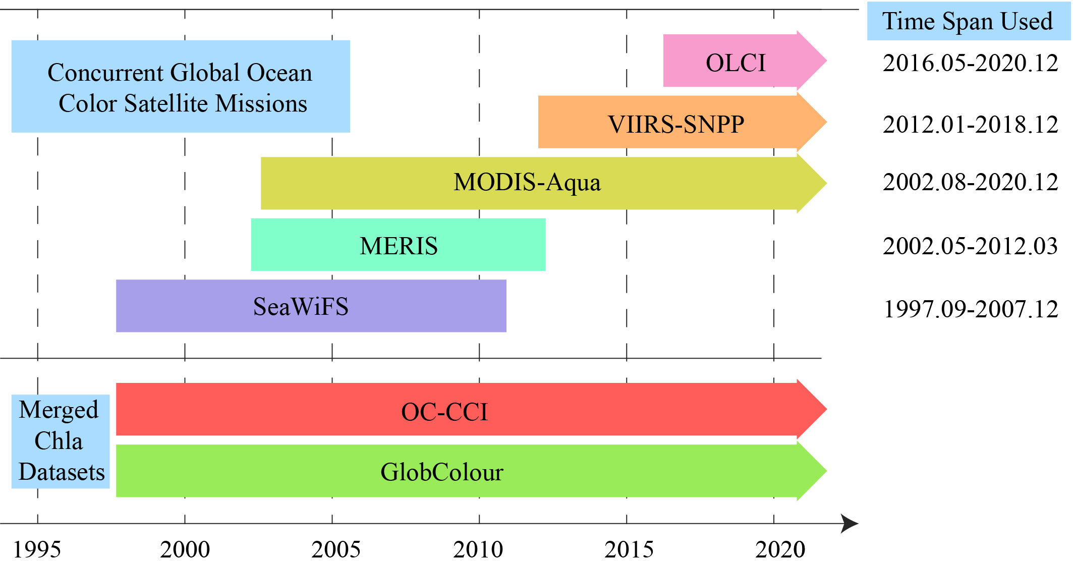
Figure 1 The time span of sensors and merged datasets.

An effective way to assess and validate the quality of our merged product is to compare it with other datasets. The merged Chla dataset we produced will be compared with two merged Chla products, the OC-CCI and GlobColour datasets. The ESA climate office provided the OC-CCI 8-day and monthly Chla products (version 5.2) with a 4-km resolution for 1997–2020 (https://climate.esa.int/en/projects/ocean-colour/). For GlobColour, as the weighted averages of single sensors have apparent disadvantages in ensuring the authenticity of the Chla trend detected, just like switching from one sensor to another at a particular point of time, we employed the GSM product rather than the AVW product. The GlobColour data (http://globcolour.info/) used in this study are the Level-3 gridded data, which are 8-day and monthly averages with a resolution of 4 km and developed, validated, and distributed by ACRI-ST, France.

To validate the accuracy of Chla data retrieved by the product, we adapted the global bio-optical in situ database constructed for ocean-color satellite remote sensing published by Valente et al. (2019). The database was composed of different sources, including MOBY (Marine Optical Buoy), BOUSSOLE (BOUée pour l’acquiSition de Séries Optiques à Long termE project), AERONET-OC (AErosol RObotic NETwork-Ocean Color), SeaBASS (SeaWiFS Bio-optical Archive and Storage System), NOMAD (NASA bio-Optical Marine Algorithm Dataset), MERMAID (MERIS Match-up In situ Database), AMT (Atlantic Meridional Transect), ICES (International Council for the Exploration of the Sea), HOT (Hawaii Ocean Time-series), and GeP&CO (Geochemistry, Phytoplankton, and Color of the Ocean), with an increased number of matchups with satellite records and spatiotemporal distribution. The compiled data span the period from 1997 to 2018 and have a total data volume of 79,924 samples. This dataset was initially built to develop and validate OC-CCI products (Sathyendranath et al., 2019).

Additionally, to illustrate the potential driving mechanism of climate change to the long-term trends of Chla, trends in sea surface temperature (SST) are presented in the discussion section. The monthly SST data were obtained from the AVHRR_OI (optimal interpolation) dataset (processing version 2.1) provided by the Group for High-Resolution Sea Surface Temperature, National Oceanic and Atmospheric Administration (https://www.ghrsst.org/), and have a 0.25° resolution.

2.2 Method of merging multiple sensors

The data-merging algorithm we built is for Level-3 Chla records. Space agencies have expended considerable effort on the calibration of instruments and assessing their stability over time, thus supporting a solid basis for using single-mission Chla products as reliable references for multi-annual time-variation analysis (Xiong et al., 2009; Eplee et al., 2012; Cao et al., 2013; IOCCG, 2013; Eplee et al., 2015; Mélin, 2016). Therefore, we adopted an efficient inter-mission bias-correction method that minimizes the trend signal modification from every single sensor. The principle of this method entails correcting inter-mission bias between two sensors using their overlapping observation period. This merging strategy was mentioned by Mélin et al. (2017) and used to build a standard sequence in which inter-mission biases between SeaWiFS and MODIS/Aqua were considered to be corrected to check the impact of inter-mission differences and drifts on Chla trend estimates. On this basis, we extended this method to the above five sensors and produced global monthly and 8-day-averaged Chla products from September 1997 to December 2020. The data production procedure is shown in Figure 2.

FIGURE 2

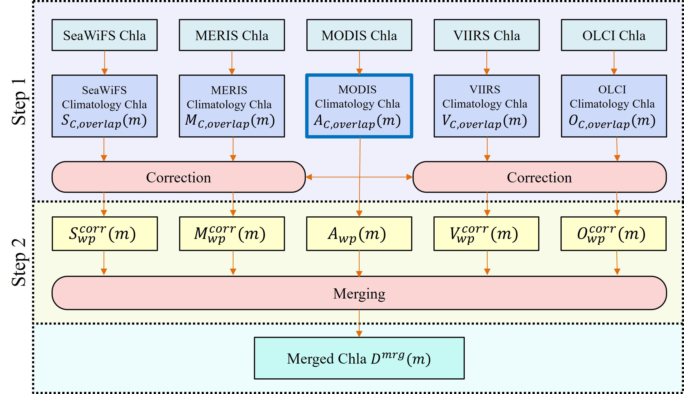
Figure 2 The procedure of multiple sensors Chla data merging.

Because of the long on-orbit operation time of MODIS/Aqua(A) (i.e., from August 2002 to the present), the overlap with SeaWiFS(S), MERIS(M), VIIRS(V), and OLCI(O) is more than five years, so MODIS/Aqua is regarded as the benchmark in this work. The first step is bias correction, which corrects the data derived by other sensors. For each pixel, the inter-mission bias between MODIS/Aqua (A) and the target sensor (X), Δ_A, X , can be expressed as

$${\text{Δ}}_{A, X}\left(m\right)=A_{C,overlap}\left(m\right)- X_{C,overlap}\left(m\right)$$

where we use monthly data for example, m means the monthly data that were processed, and the ‘C, overlap’ subscript indicates the climatological monthly Chla derived using the overlap period for the 8 days or month m. Taking SeaWiFS as an example, we see that the climatological January value is the average of the valid January values for the five years overlapping with MODIS, from 2003 to 2007, and so on for the other months and sensors. The corrected record of sensor X, $X_{wp}^{corr}\left(m\right)$, can be expressed as

$$X_{wp}^{corr}\left(m\right)=X_{wp}\left(m\right)+{\Delta }_{A, X}\left(m\right)$$

where the ‘wp’ subscript means the whole on-orbit period of sensor X, and X_wp (m) represents the entire original series of the target sensor X. The first step corrects the spatial and seasonal dependencies in inter-mission biases that have been noticed for ocean-color products in a simple manner and guarantees consistency for the merged Chla product (Mélin, 2016; Sathyendranath et al., 2019). Some negative values could result from considering the bias as an arithmetic difference, but the number of negative values is quite limited in practice, accounting for an average of 0.91% of the total valid pixels for SeaWiFS, 1.33% for MERIS, 0.18% for VIIRS, and 0.97% for OLCI. These negative values are regarded as invalid data and excluded from subsequent processing.

In the second step, merging is simply averaging the available data for a given pixel. Therefore, the merged series, D^mrg (m), can be expressed as

$$D^{mrg}\left(m\right)=\frac{1}{N}\sum _{i=1}^{N}X\left(m\right)$$

where N represents the number of sensors in orbit for each month m and X (m) indicates the corrected Chla of every single sensor and MODIS record.

2.3 Calculation of time-series trends

Trends showed in this work were based on linear regression analysis of monthly Chla anomaly data. Using anomaly data instead of monthly Chla data helps to avoid the interference of seasonal signals on interannual trend detection. The monthly anomaly sequence was obtained by subtracting the corresponding monthly climatological value from the monthly value. The anomaly sequence and corresponding date (e.g., months since the first month) were linearly fitted pixel by pixel, and the obtained slope is then regarded as the rate of change of Chla in units of μg/L/month, which is converted to μg/L/yr subsequently. For a certain region, we first calculate the regional average Chla value, and then obtain the anomaly sequence and calculate the trend at last. A statistically significant trend is one that exceeds the 95% confidence level (i.e., p< 0.05) under the t-test.

2.4 In situ data matchup

The in situ Chla data (Valente et al., 2019) were matched with corresponding satellite data to validate the merged products. First, the in situ data were gridded with a time window of 8 days and a spatial window of 4 km, the same as the satellite data resolution. The principle is that each sample can only belong to one grid. For the grid containing more than three samples, abnormal values were identified by the 3σ principle and eliminated. The averaged value of valid data in each grid was considered as the value of the grid. Then, matching-up processing basically followed the procedures adopted by the OC-CCI group (Sathyendranath et al., 2019): The nearest latitude and longitude identified the central pixel collocated with each in situ datum. The surrounding pixels (a 5 × 5 box with the in situ datum in the center) were selected for further analysis. Only those pixels with a valid central pixel and satisfying checks that Chla was within the 0.01–100 μg/L range and at a water depth of >50 m according to bathymetry were considered to be valid. Homogeneity criteria—that the coefficient of variation was<0.15 and at least 10 valid pixels were in the 5 × 5 box—were also used to exclude nonhomogeneous pixels to avoid the impact of the noise within satellite products on the validation. In addition, high-latitude ocean regions (>66.5°) are excluded owing to the generally high Chla values in these regions that are not applicable for the CI-based Chla algorithm (Wang and Son, 2016). Finally, valid central pixels and corresponding gridded in situ data were matched to construct the database for product validation.

3 Results

3.1 Validation by in situ Chla data

Comparison with in situ measurements is one of the essential means of validating the quality of satellite products (Maritorena et al., 2010). After the procedures mentioned in section 2.4 were implemented, 19,836 groups of in situ data matched up with our product. As a reference, OC-CCI and GlobColour products were also involved. Finally, 15,599 groups of valid data were successfully matched with all OC-CCI, GlobColour, and our products. Their spatial and numerical distributions are shown in Figure 3.

FIGURE 3

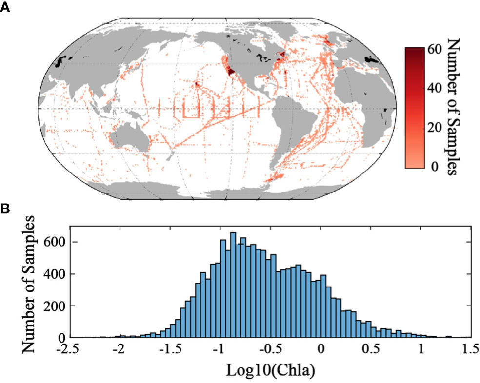
Figure 3 (A) Spatial and (B) numerical (bar plot) distribution of in situ Chla data matched up for the OC-CCI, GlobColour, and our merged products (15,599 in total); (Units of Chla: μg/L.).

Figure 4 shows how the three merged 8-day products compare with the corresponding gridded in situ observations. It indicates an acceptable agreement between the product generated in our study and the in situ data (Figure 4A), with a root mean squared error (RMSE) of 1.04 and R² = 0.75 based on log₁₀ Chla. The statistics are similar to that of OC-CCI and GlobColour (Figures 4B, C), whose RMSE values are 0.98 and 0.91 and R² values are 0.78 and 0.79, respectively. The low degree of correlation may be because the sampling time of the in situ observations does not entirely match that of the satellite data (8 days) despite the gridding before matching up. Though no in situ observations were employed in the data processing, the accuracy of the Chla value of this work is not inferior to that of OC-CCI and GlobColour data. Validations with all the matched samples for three individual products were presented in Supplementary Material Figure S1, which also showed that the three products have similar accuracy, despite different matchup samples owing to different spatial coverage.

FIGURE 4

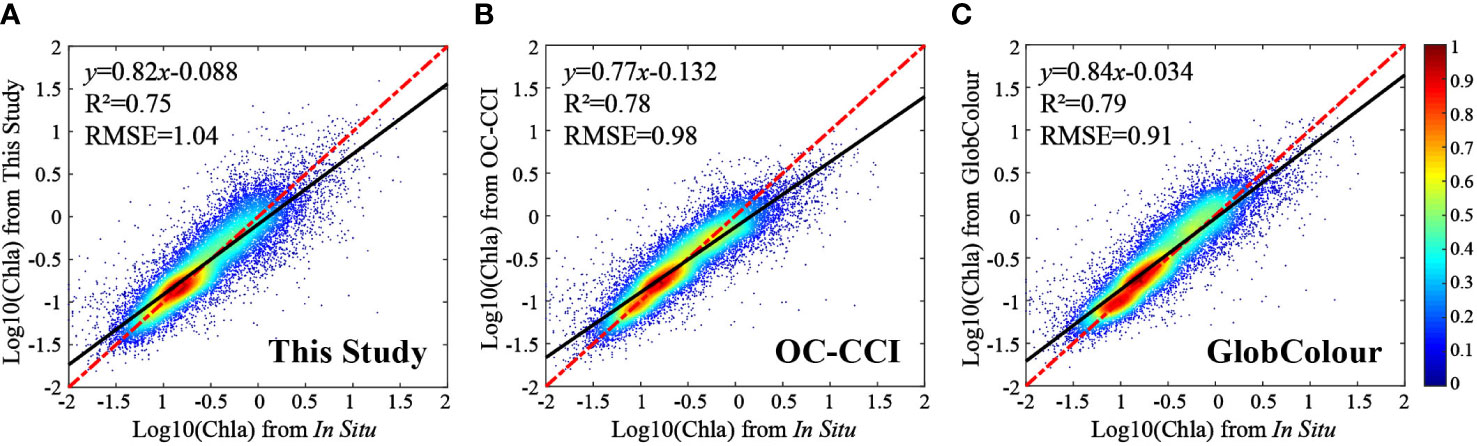
Figure 4 Comparison of in situ Chla data with the corresponding 8-day and merged satellite data from (A) this study, (B) OC-CCI, and (C) GlobColour. The color scale indicates the data density in pixels, the black lines are the linear fitting of in situ and satellite data, and the red dotted lines represent 1:1. Log10(Chla) was used in the computation of the fitted equation and R². Chla was used in the computation of RMSE. (Units of Chla: μg/L.).

3.2 Trend validation by using the original sensor sequence

This work is oriented toward producing a set of global satellite-derived Chla products with high reliability on the long-time-series trend analysis. Under the assumption that single sensors can be used as a benchmark time series as the trends they capture are the actual variability of Chla, the dataset we produce should be able to reproduce the trend patterns obtained by single-mission records over their respective periods. Mélin et al. (2017) proposed a protocol to assess the fitness of OC-CCI Chla data (version 3.0) using contingency matrices, Cohen’s κ index, and the differences (and their distributions) between trend slopes. Contingency matrices were used to compare the trends (expressed in terms of significant increase, significant decrease, and not significant) associated with two satellite products. Cohen’s κ index is used to quantify the magnitude of the agreement between two diagnostics (Cohen, 1960; Viera and Garrett, 2005; Warrens, 2011); the more κ value close to 1, the more consistent two diagnostics are. Here we apply the main principle of this protocol suggested by Mélin et al. (2017) to assess our dataset by comparing it with single sensor records.

3.2.1 Comparison with SeaWiFS for September 1997 to December 2007

The contingency matrix comparing trends derived by SeaWiFS and this study over the overlapping period (September 1997 to December 2007) is presented in Table 1. The diagnostics agree; that is, the slopes of linear regression S of both sequences are concurrently greater than 0 (Chla increase), less than 0 (Chla decrease), or not significant for >91.91% of the ocean over which the trend diagnostics apply (with 66.29% associated with nonsignificant trends and 25.62% associated with significant trends). Contradictory diagnostics characterize only 8.09% of the domain, and the worst case, in which significant trends for both products have opposite signs, almost never occurs (being found in only two pixels). The same comparisons were conducted on OC-CCI and GlobColour products (Table 1); 80.97% and 82.16% of the areas exhibit consistent diagnostics, respectively, both of which are ∼10% lower than that in this study. The κ values of three products were 0.82, 0.59, and 0.63, respectively.

TABLE 1

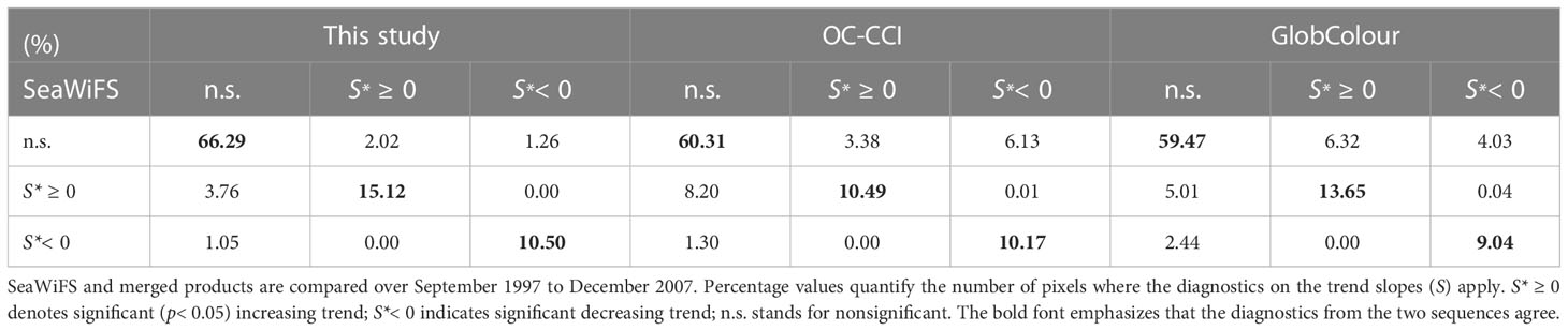
Table 1 Contingency matrices comparing trend analysis outcomes for SeaWiFS period.

In addition to the consistency of diagnostics, the value of Chla trends was also validated. Figures 5A–C show the pixel-by-pixel comparison between the rate of change derived from SeaWiFS and that of the three merged products. It can be seen that the rate of change found in this study is most consistent with that of SeaWiFS at the pixel level (Figure 5A), with R² = 0.93 and RMSE = 0.008. The numerical distribution of the rate of change from OC-CCI is relatively discrete (Figure 5B), with R² = 0.20 and RMSE = 0.034, and the absolute value of which is underestimated compared with that of SeaWiFS. The rate of change of GlobColour is concentrated around 0, and the increasing trend is significantly underestimated (R² = 0.30 and RMSE = 0.024, Figure 5C).

FIGURE 5

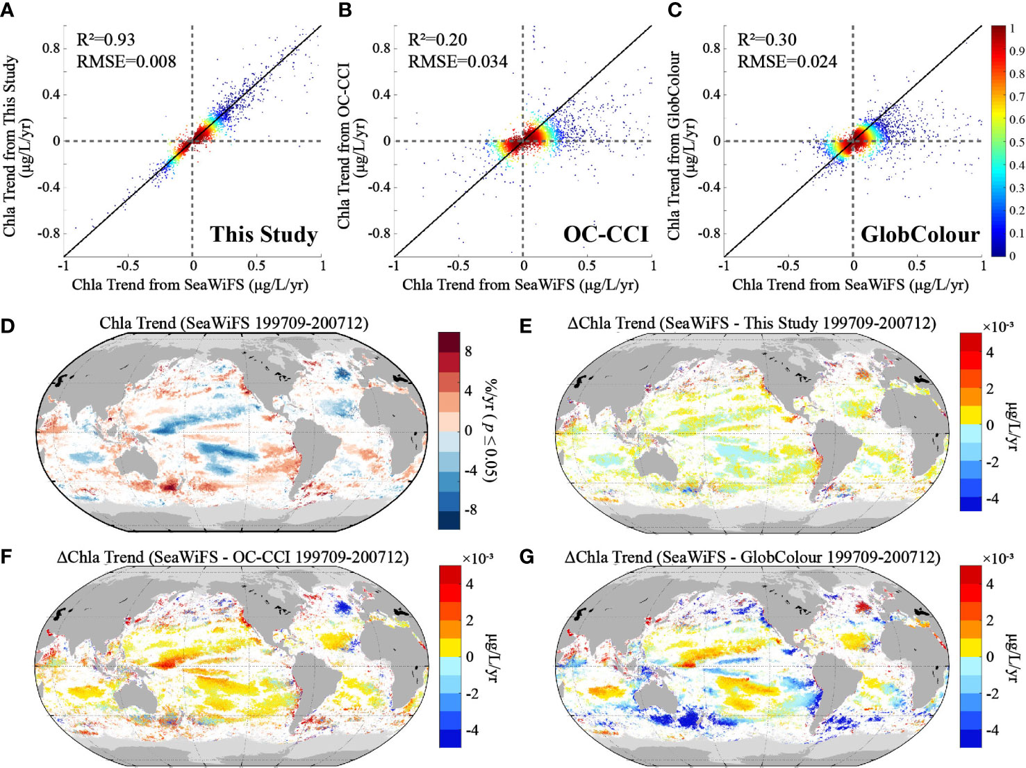
Figure 5 (A–C) Scatter plots of pixel-by-pixel Chla trends comparison between SeaWiFS and the three merged datasets from September 1997 to December 2007. (D) Chla trend maps in units of %/yr from SeaWiFS for September 1997 to December 2007. (E–G) Chla trends from SeaWiFS minus that from the three merged datasets in units of μg/L/yr. Black lines on the scatter plots represent the 1:1 line, and the color scale indicates the data density in pixels. The light gray on the maps represents insufficient data for making a trend calculation (i.e., the number of valid data collected in the statistical period (62 months) does not reach 50%), and the white color indicates that the SeaWiFS data show that the pixel has not changed significantly (p< 0.05).

The global distribution of ocean Chla variation from September 1997 to December 2007 derived from the SeaWiFS record is shown in Figure 5D. The regions with significant increases of Chla are mainly located in the Northwest Pacific, the edge of the South Pacific Basin, the South Atlantic, and the western North Indian Ocean, and the regions with decreases are concentrated in the North Atlantic, the center of the South Pacific Basin, the subtropical North Pacific, and the eastern Indian Ocean (Figure 5D). The spatial distributions of the differences between the rates of change from the SeaWiFS record and that of the merged products are shown in Figures 5E–G. The trends generated from this study are more consistent with that of the SeaWiFS record, with the differences ranging within ±2 × 10⁻³ μg/L/yr and slightly underestimating the growth rate in the mid and high latitudes of the northern hemisphere, the Arabian Sea, and the west coast of South America (Figure 5E). However, OC-CCI records in this period exhibit a noticeable disagreement, with the difference being generally positive. Specifically, the decreasing trends of Chla in the Pacific Ocean, Indian Ocean, and North Atlantic oligotrophic basin are overestimated, and the increasing trends in the South Pacific Basin, Arabian Sea, and coastal oceans are underestimated (Figure 5F). GlobColour underestimates the increasing trends of the Southern Ocean and along the margin of the Pacific and the decreasing trends of the oligotrophic basin to a great extent (>4 × 10⁻³ μg/L/yr, Figure 5G).

3.2.2 Comparison with MERIS for May 2002 to March 2012

Validations of the trend diagnosis, value, and distribution of trend differences were conducted by taking the MERIS record as a benchmark over the period of May 2002 to March 2012 similarly. As Table 2 indicates, the slopes of our product agree with the MERIS record for 85.94% of the ocean, representing the most incredible consistency among the three products. The portion is 11.05% and 5.68% higher than that of OC-CCI and GlobColour. The κ values of the three products were 0.70, 0.50, and 0.59, respectively, also indicating that our product has the highest agreement in trend diagnosis with MERIS.

TABLE 2

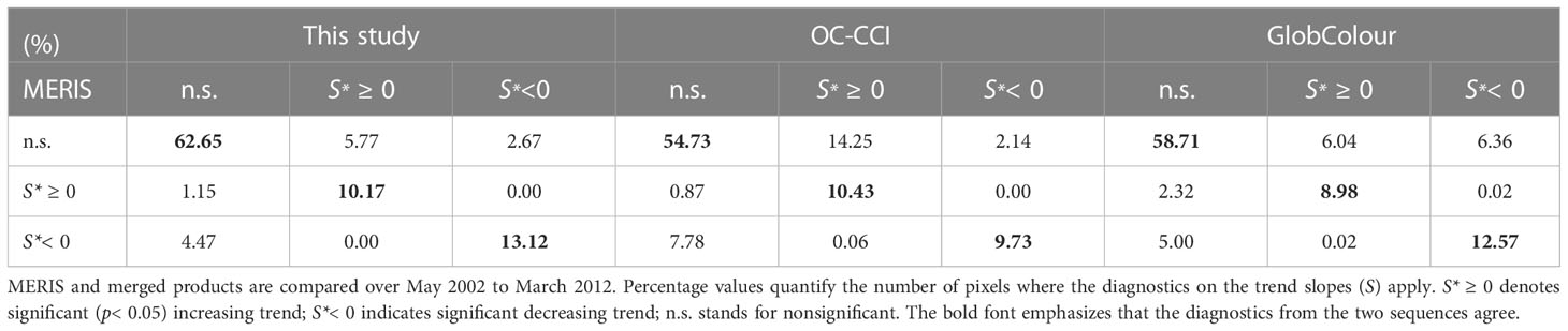
Table 2 Contingency matrices comparing trend analysis outcomes for MERIS period.

As to the value of the trend, the trend from our product is the most consistent with the MERIS sequence, with the highest R² and lowest RMSE (Figure 6A). The slopes of the other two products have significant systematic bias and are concentrated near 0 (Figures 6B, C).

FIGURE 6

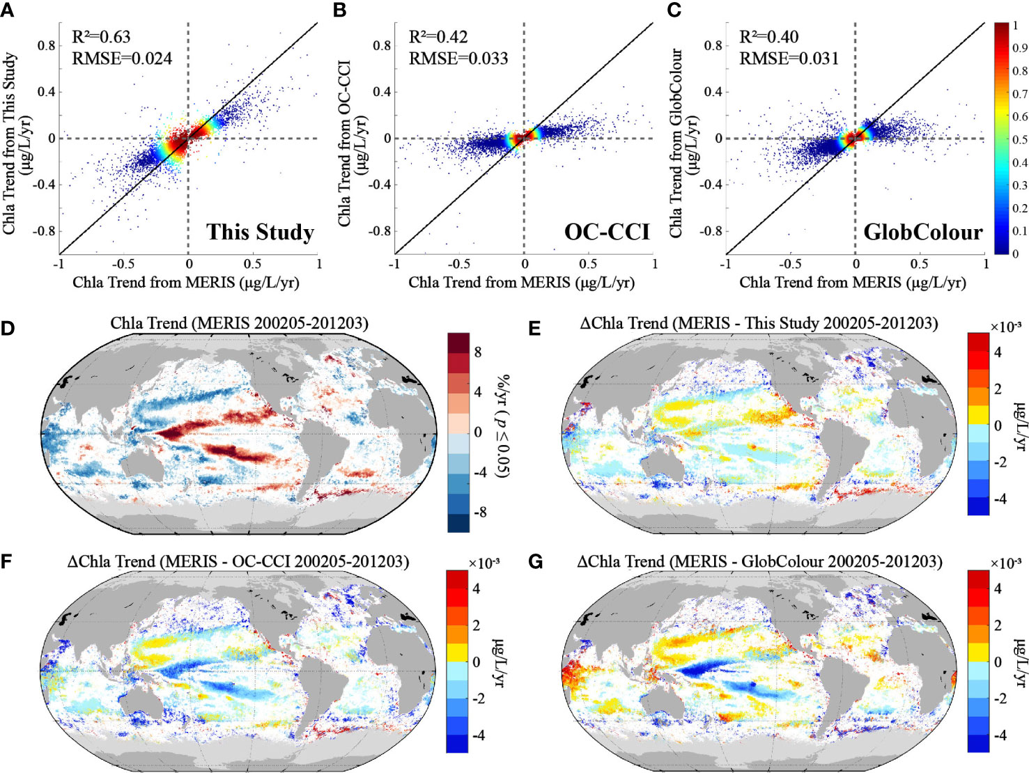
Figure 6 Pixel-by-pixel comparison of the Chla rate of change from MERIS and (A) this study, (B) OC-CCI, and (C) GlobColour. (D) Chla trend maps in units of %/yr from MERIS for May 2002 to March 2012. (E–G) Chla trends from MERIS minus that from the three merged datasets in units of μg/L/yr. Black lines on the scatter plots represent the 1:1 line, and the color scale indicates the data density in pixels. The bright gray on the maps represents insufficient data for estimating a trend (i.e., the number of valid data collected in the statistical period (60 months) does not reach 50%), and white indicates that the MERIS data show that the pixel has not changed significantly (p< 0.05).

The trend map for the MERIS record (Figure 6D) shows that Chla increased dramatically at a rate of 5%–10%/yr in the low-latitude basin of the Pacific Ocean while decreasing in the western Indian Ocean and mid-latitude basins in the Pacific and Indian oceans by 5%–8%/yr throughout May 2002 to March 2012. Trends generated from this study have minor differences from that of the MERIS record, ranging mostly within ±2 × 10⁻³ μg/L/yr and underestimating the increasing trend in the mid- to low-latitude basin and the area near 60°S in the eastern Pacific (Figure 6E). Both OC-CCI and GlobColour dramatically overestimated the growing trend by >3 × 10⁻³ μg/L/yr in the low-latitude basin of the Pacific Ocean compared to the MERIS record (Figures 6F, G). Moreover, GlobColour also overestimated the decreasing trend in the western Indian Ocean.

3.2.3 Comparison with VIIRS for 2012 to 2018

In the case of VIIRS records throughout January 2012 to December 2018 (Table 3), our product and GlobColour have better diagnostic consistency with VIIRS, as the diagnostic trends are consistent in 82.74% and 85.73% of regions and with κ values 0.61 and 0.68 (versus only 74.8% and 0.46 for OC-CCI).

TABLE 3

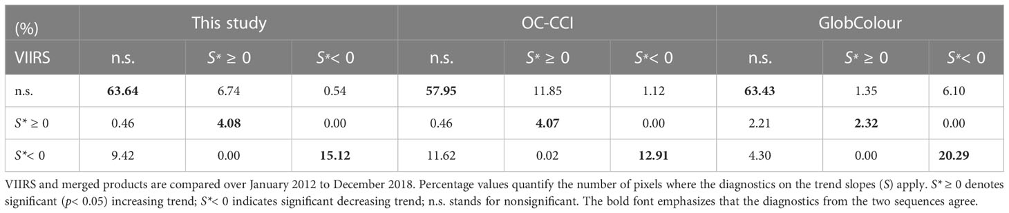
Table 3 Contingency matrices comparing trend analysis outcomes for VIIRS period.

It can be seen that the consistency between our product and VIIRS is better than that for the other two products at the pixel level (Figure 7A). The numerical distribution of the Chla trends from OC-CCI is concentrated (Figure 7B), and, for GlobColour, it is relatively discrete but tends to be negative overall (Figure 7C).

FIGURE 7

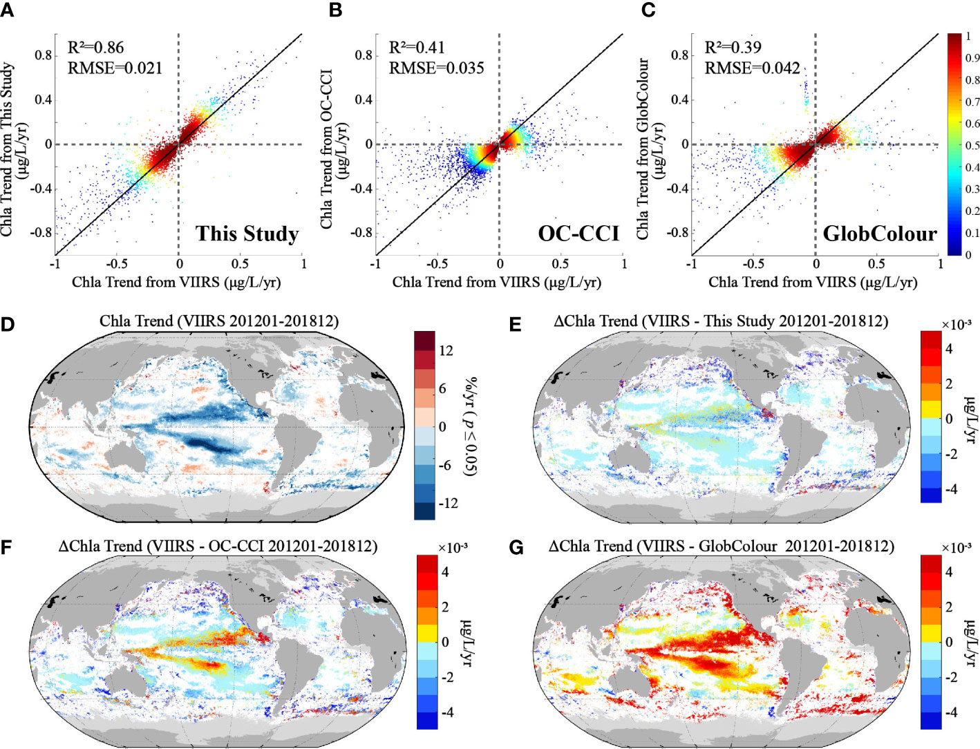
Figure 7 Pixel-by-pixel comparison of the Chla rate of change from VIIRS and (A) this study, (B) OC-CCI, and (C) GlobColour. (D) Chla trend maps in units of %/yr from VIIRS for January 2012 to December 2018. (E–G) Chla trends from VIIRS minus that from the three merged datasets in units of μg/L/yr. Black lines on the scatter plots represent the 1:1 line, and the color scale indicates the data density in pixels. The bright gray on the maps represents insufficient data for trend estimation (i.e., the number of valid data collected in the statistical period (41 months) does not reach 50%), and white indicates that the VIIRS data show that the pixel has not changed significantly (p< 0.05). .

The Chla records from VIIRS exhibit a significant negative trend overall from 2012 to 2018, especially in the Pacific low-latitude basin and the northeast Pacific marginal seas, with declining trends of >10%/yr (Figure 7D). Though our study generally underestimated the declining trend, the difference with VIIRS is slight, primarily within 2 × 10⁻³ μg/L/yr (Figure 7E). OC-CCI overestimates the decreasing rate in the mid and low latitudes of the Pacific to a large extent, but the rate is similar to that of our product in other regions (Figure 7F). GlobColour exhibits apparent bias, which leads to a significant overestimate of the declining trend worldwide by >4 × 10⁻³ μg/L/yr (Figure 7G).

Comparison with MODIS is shown in Supplementary Material (Table S1 and Figure S2). Since the MODIS record is used as a baseline in this study, the trends derived from our dataset are much more consistent with that from MODIS than OC-CCI and GlobColour.

4 Discussion

4.1 Global Chla trend

The trends obtained for SeaWiFS (September 1997 to December 2007), MERIS (May 2002 to March 2012), and VIIRS (January 2012 to December 2018) are presented in Figures 5D, 6D, 7D, respectively. It is noticeable that the oligotrophic subtropical gyres in the Pacific witnessed significant negative trends from late 1997 to 2007, which was also mentioned in several previous studies (Vantrepotte and Mélin, 2009; Vantrepotte et al., 2011; Vantrepotte and Mélin, 2011). However, these trends were replaced by a positive signal in the following period, as Mélin et al. (2017) reported, and then reverted to a negative trend again. Transformations in trend also occurred in the north temperate Pacific and the western Indian Ocean, where Chla values exhibited an increasing trend before 2008 and then decreased afterward.

Time-series analysis for single sensors is limited to about ten years, while merged products enable trend detection over decades. Here we employed our product to calculate global Chla changes for 23 years (1998–2020, Figure 8A). Significant negative trends (which can reach −1% to −2% per year) are generally observed in the Pacific and Indian oligotrophic gyres. In contrast, significant positive trends are noticed in various regions, including the Southern Ocean, Southeast Pacific, South Atlantic gyres, and isolated patches in the north Arabian Sea and mid to high latitudes of the northern hemisphere.

FIGURE 8

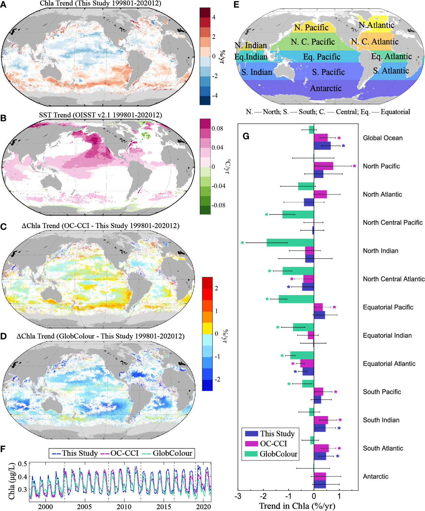
Figure 8 (A) Chla trend map derived from this study and (B) SST trend map from 1998 to 2020. (C, D) Trend differences between OC-CCI and GlobColour and that from this study in units of %/yr. (E) Basin definitions for the trend analysis (Gregg and Rousseaux, 2014), (F) time series curve of global Chla, and (G) Chla trends in global oceans and 14 basins from the three merged datasets. The light gray on the maps represents insufficient data from our dataset for making a trend calculation (i.e., the number of valid data collected in the statistical period (138 months) does not reach 50%), and white indicates that the pixel trend is insignificant (p > 0.05) according to our dataset. For (G), the bar with an asterisk (*) marked indicates that the trend is significant (p< 0.05); error bars show 95% credible intervals of the rate of change.

Figure 8B shows the SST trend during this period. The SST in the Indian Ocean, the Northwest Atlantic, the mid- and low-latitude ocean basin and the northeastern part of the Pacific, including the Bering Sea, increased significantly. The sea area between 45°S–60°S of the Southern Ocean also became warmer. The negative trends in Chla in the subtropical oligotrophic gyres appeared to be consistent with the hypothesis of a more stratified and warming ocean (Doney, 2006). Increasing temperature strengthens the stratification of the upper ocean, which hinders the nutrient supply from the subsurface to the upper layer, thereby limiting phytoplankton growth and decreasing Chla (Behrenfeld et al., 2006; Irwin and Oliver, 2009; Behrenfeld et al., 2016). However, the increasing temperature in the middle to high latitudes could promote phytoplankton growth by becoming closer to the optimum growing temperature for some phytoplankton species (Thomas et al., 2012) and causing poleward shifts of phytoplankton communities at mid to low latitudes (Toggweiler and Russell, 2008; Gregory et al., 2009), thus leading to the increase in Chla here. Moreover, the generally positive trend of Chla in the Southern Ocean is also consistent with the widely reported conclusion that carbon sinks have increased significantly since 2000 (Lavender et al., 2015; DeVries et al., 2019; Gruber et al., 2019; Zhang et al., 2022).

Our product indicates that the global pelagic ocean Chla presented a significant increasing trend over 1998–2020 with a rate of 0.67% ± 0.37%/yr, which is a more positive value than found in a number of previous studies. Using the SeaWiFS record, Vantrepotte and Mélin (2011) found that, over the period 1997–2007, Chla decreased in most of the global ocean; our results from SeaWiFS original series are consistent with these findings (Figure 5D). Saulquin et al. (2013) reported a low-magnitude positive trend (2.83 × 10⁻⁴ μg/L/yr) in global Chla over September 1997 to April 2012 using combined data from SeaWiFS and MERIS. However, Hammond et al. (2017) calculated that the trend of marine Chla from September 1997 to December 2013 was −0.023% ± 0.12%/yr using the Bayesian hierarchical spatiotemporal model and the OC-CCI dataset. They further reported a global average weighted trend of 0.08 ± 0.35%/yr over the period 1997–2018 with prior information provided by the Coupled Model Intercomparison Project phase 5 output (Hammond et al., 2020). It is reasonable to get different trends when various periods and datasets are analyzed.

The global data were further divided into 12 regions (Figure 8E) according to Gregg and Rousseaux (2014) to quantify the Chla trend. Significant declines are observed in the North Central Atlantic and equatorial Atlantic, whereas, in the South Indian and South Atlantic oceans, Chla increases by 0.5%/yr. The downward trend in the North Atlantic was earlier mentioned by Gregg and Rousseaux (2014), who integrated SeaWiFS and MODIS records from 1998 to 2012 and reported that the rate of decline was 1.1%/yr. The rate of the decreasing trend we calculated for the North and Central Atlantic is much lower, being 0.46% ± 0.42%/yr. The differences could be attributed to the different datasets and the eight-year longer data span we used. The decline in the equatorial Atlantic (0.45% ± 0.17%/yr) is consistent with the result of Hammond et al. (2018), who, using the OC-CCI record, suggested that Chla in the Eastern Tropical Atlantic decreased by ~0.7%/yr from 1998 to 2016. The increased Chla in the South Indian and South Atlantic oceans may be associated with relatively stable temperature (Figure 8B) and stratification, as well as atmospheric soluble iron deposition enhancement (Hamilton et al., 2020).

In addition, it is worth noting that, from the trend map, many of the pixels in the North Pacific, North Atlantic, North Indian, and Antarctic oceans exhibit a significant increasing trend, but not from the perspective of the regional statistics. One possible reason for this difference is that, during data processing, we first calculate the regional average value of each month, and then we calculate its linear trend. The increasing signal may be interfered with or masked when the pixels that significantly declined and nonsignificantly changed (which also account for a considerable proportion) were also included in regional averaging. Another possible cause is the different data coverage before and after 2002 (Gregg and Casey, 2007). Before 2002, the spatial coverage of the merged data was relatively insufficient as only SeaWiFS was in orbit, while at least two sets of satellite data were available at the same time after 2002, especially the introduction of MERIS and the processing of MERIS data with POLYMER (Steinmetz et al., 2011; van Oostende et al., 2022), improved the spatial coverage of the data considerably, especially in high latitudes, the intertropical convergence zone, and highly productive coastal regions. The data before 2002 may not represent the whole region with insufficient coverage, thus misleading the trend calculation. This problem exists in basically all multimission ocean-color datasets. However, (van Oostende et al., 2022) applied the temporal gap detection method (TGDM) to the OC-CCI record to homogenize the observations per pixel of the time series, which may be worth attempting to avoid artifacts trends in long-term analysis when significant coverage differences exist in the interested regions.

4.2 Trend difference between merged Chla datasets

Many studies on the trend of the Chla long-time series use the products from OC-CCI and GlobColour (Chen et al., 2014; Racault et al., 2015; Hammond et al., 2017; Sravanthi et al., 2017; Gbagir and Colpaert, 2020; Hammond et al., 2020; Moradi, 2021; Guo et al., 2022). Mélin et al. (2017) assessed the fitness for time-series analysis of OC-CCI Chla data (version 3, 1998–2015) and stated that the OC-CCI data had a remarkable agreement with single-mission products. However, it should not be taken for granted, as the results have evolved with the OC-CCI dataset versions (Mélin et al., 2017). Hammond et al. (2018) assessed the presence of discontinuities in both the OC-CCI dataset (version 3.1) and the GlobColour dataset from September 1997 to December 2016 and found their effect in most regions worldwide, which leads to a corresponding difference in trend estimates, with a maximum difference of 2.9%/yr, and can even change the direction of trends.

In Section 3.2, we verified that our merged product has acceptable accuracy of the Chla value and fits to long-term Chla trend analysis and climate change related studies better than OC-CCI and GlobColour products as it is more consistent with the single-satellite sequence in the aspect of trend diagnosis. Figures 8C, D show the difference between the Chla variation rate calculated in this study and that of the two published merge products from 1998 to 2020. OC-CCI may overestimate the rising rate by 0.5%–1% per year in the Southern Ocean and Southeast Pacific, lose sight of the increase in the northwest Arabian Sea, and underrate the rising observed along the Northwest Pacific margin. GlobColour, however, shows an overall negative pattern, that is, an overstated downward trend over the Pacific and Indian oligotrophic gyres, an underestimated increasing rate at the North Atlantic high latitudes, Southern Ocean, and Southeast Pacific, and even a misdiagnosed growing trend in the north Arabian Sea and South Atlantic.

The global ocean Chla trend from OC-CCI is similar to that from our product, with a rising rate of 0.54% ± 0.31%/yr, while the trend from GlobColour indicates that it had not changed significantly (Figure 8G). The noticeable discontinuity can be captured from the global time-series Chla curve (Figure 8F) of OC-CCI and GlobColour with systematical high values over 2002–2012 resulting from the introduction of MERIS and the utilize of POLYMER to MERIS data (Steinmetz et al., 2011; van Oostende et al., 2022). In addition, GlobColour also has an obvious systematic low value after 2017. In terms of regional statistics, OC-CCI exhibits the same trends in regions where significant trends occurred according to our dataset, with slight differences in the rate of change (~0.1%/yr). It also indicates that Chla increased in the North, equatorial, and South Pacific oceans while there was no significant trend detected from our dataset. GlobColour exhibits overwhelming negative trends in most regions (7 out of 12) besides high latitudes, with no positive trend found. It should be noted that the decreasing trend revealed by GlobColour in the North Central, equatorial, and South Pacific oceans and the North and equatorial Indian oceans was not found in OC-CCI nor in our product. In general, the Chla trend generated from OC-CCI is closer to that from our products compared with GlobColor because the OC-CCI dataset has been corrected for Rrs bias (Lavender et al., 2015), while the GlobColour data are not explicitly bias-corrected but are instead merged by inversion with a bio-optical model (Maritorena et al., 2010).

5 Conclusions and implications

To better detect the long-term trend of sea surface Chla, we corrected and merged multi-sensor Chla data and produced a set of satellite-derived Chla products from September 1997 to 2020. Our product has similar accuracy to that of OC-CCI and GlobColour products in terms of Chla value, as has been validated by the in situ data. Moreover, the dataset has great potential to be used in climatology studies as it has excellent accuracy in Chla trends that is generally more consistent with single-mission records than OC-CCI and GlobColour products. Based on this dataset, we illustrated the linear trend of Chla and its distribution in various regions around the world over 23 years. The difference among trends estimated using the three merged products was also analyzed to provide a reliable Chla trend and stated that caution should be exercised when using existing merged products to calculate long-term trends.

Though the method we employed to correct bias between sensors is straightforward, we have performed a series of validations to prove the fitness of the dataset in long-term ecological research. Our method is an efficient operation and is easy to apply and extend. We used MODIS records as the benchmark, but, in the future, with the launch of new satellites and the continuous accumulation of Chla data, this method can be used to build new datasets quickly. It can also be extended to other missions and parameters such as SST, kd490, and Rrs from multiple missions. However, it should be stated that the method itself tends more toward mathematics and statistics and barely involves remote-sensing mechanisms. We have also assumed that the bias between sensors does not change with the aging of sensors during the overlap period. Although we have performed quality control for single-sensor data, in theory, though limited, the aging of sensors may impact the correction effect.

The key objective of this study is to create a new dataset for better trend detection and provide a reliable trend map of Chla in the past 23 years, and we have corrected the potential misunderstanding of global Chla changes generated by the OC-CCI and GlobColour datasets. Our data have been shared on Zenodo (https://doi.org/10.5281/zenodo.7092220). We hope our work can offer the community a reliable dataset to conduct Chla trends analysis globally and on different systems, provide a methodology reference for developing future ocean-color CDR and ECV products, and thus contribute to understanding the long-term trend of phytoplankton under climate change.

Data availability statement

The datasets presented in this study can be found in online repositories. The names of the repository/repositories and accession number(s) can be found below: https://doi.org/10.5281/zenodo.7092220.

Author contributions

SY: Methodology, Visualization, Writing – original draft. YB and XH: Resources; Writing - Review & Editing. FG: Writing - Review & Editing; English writing improving. TL: Methodology; Writing - Review & Editing. All authors contributed to the article and approved the submitted version.

Funding

This study was supported by the National Natural Science Foundation of China (Grants #41825014, #42176177, and# 42141001), the National Key Research and Development Program of China (Grant #2017YFA0603003) and Zhejiang Provincial Natural Science Foundation of China (2017R52001 and LR18D060001).

Acknowledgments

We thank NASA’s Ocean Biology Processing Group (OBPG) and Ocean Color website (https://oceancolor.gsfc.nasa.gov/. Accessed on 17 December 2021) for providing the level-3 gridded chlorophyll concentration data derived from SeaWiFS, MODIS/Aqua, and VIIRS/SNPP. We thank ESA’s GlobColor Project (https://hermes.acri.fr/. Accessed on 29 December 2021) for providing the level-3 gridded chlorophyll concentration data derived from MERIS and OLCI/Sentinel-3A and merged chlorophyll concentration dataset. We thank ESA’s Ocean Colour Climate Change Initiative (OC-CCI) and the climate office (https://climate.esa.int/en/projects/ocean-colour/. Accessed on 23 December 2021) for providing the merged chlorophyll concentration dataset. We thank National Oceanic and Atmospheric Administration’s Group for High-Resolution Sea Surface Temperature (https://www.ghrsst.org/. Accessed on 10 March 2022) for providing the AVHRR_OI (optimal interpolation) sea surface temperature dataset. We thank China’s State Key Laboratory of Satellite Ocean Environment Dynamics(SOED), Second Institution of Oceanography(SIO), Ministry of Natural Resources (MNR) satellite ground station, satellite data processing and sharing center, and the marine satellite data online analysis platform (SatCO2) for their help with data collection and processing. Special thanks are given to the editor and the two reviewers for their useful comments and constructive suggestions.

Conflict of interest

The authors declare that the research was conducted in the absence of any commercial or financial relationships that could be construed as a potential conflict of interest.

Publisher’s note

All claims expressed in this article are solely those of the authors and do not necessarily represent those of their affiliated organizations, or those of the publisher, the editors and the reviewers. Any product that may be evaluated in this article, or claim that may be made by its manufacturer, is not guaranteed or endorsed by the publisher.

Supplementary material

The Supplementary Material for this article can be found online at: https://www.frontiersin.org/articles/10.3389/fmars.2023.1051619/full#supplementary-material

References

Behrenfeld M. J., O’Malley R. T., Boss E. S., Westberry T. K., Graff J. R., Halsey K. H., et al. (2016). Revaluating ocean warming impacts on global phytoplankton. Nat. Climate Change 6 (3), 323–330. doi: 10.1038/nclimate2838

CrossRef Full Text | Google Scholar

Behrenfeld M. J., O’Malley R. T., Siegel D. A., McClain C. R., Sarmiento J. L., Feldman G. C., et al. (2006). Climate-driven trends in contemporary ocean productivity. Nature 444 (7120), 752–755. doi: 10.1038/nature05317

PubMed Abstract | CrossRef Full Text | Google Scholar

Bojinski S., Verstraete M., Peterson T. C., Richter C., Simmons A., Zemp M. (2014). The concept of essential climate variables in support of climate research, applications, and policy. Bull. Am. Meteorological Soc. 95 (9), 1431–1443. doi: 10.1175/BAMS-D-13-00047.1

CrossRef Full Text | Google Scholar

Cao C., Xiong J., Blonski S., Liu Q., Uprety S., Shao X., et al. (2013). Suomi NPP VIIRS sensor data record verification, validation, and long-term performance monitoring. J. Geophysical Research: Atmospheres 118 (20), 11,664–611,678. doi: 10.1002/2013JD020418

CrossRef Full Text | Google Scholar

Chavez F. P., Messié M., Pennington J. T. (2011). Marine primary production in relation to climate variability and change. Annu. Rev. Mar. Sci. 3, 227–260. doi: 10.1146/annurev.marine.010908.163917

CrossRef Full Text | Google Scholar

Chen X., Pan D., Bai Y., He X., Wang T. (2014). Are the trends in the surface chlorophyll opposite between the south China Sea and the bay of Bengal? Remote Sens. Ocean Sea Ice Coast. Waters Large Water Regions 9240, 270–277. doi: 10.1117/12.2067584

CrossRef Full Text | Google Scholar

Cohen J.. (1960). A coefficient of agreement for nominal scales. Educ. Psychol. Meas 20 (1), 37–46. doi: 10.1177/001316446002000104

CrossRef Full Text | Google Scholar

Collins M., An S.-I., Cai W., Ganachaud A., Guilyardi E., Jin F.-F., et al. (2010). The impact of global warming on the tropical pacific ocean and El niño. Nat. Geosci. 3 (6), 391–397. doi: 10.1038/ngeo868

CrossRef Full Text | Google Scholar

DeVries T., Le Quéré C., Andrews O., Berthet S., Hauck J., Ilyina T., et al. (2019). Decadal trends in the ocean carbon sink. Proc. Natl. Acad. Sci. 116 (24), 11646–11651. doi: 10.1073/pnas.1900371116

CrossRef Full Text | Google Scholar

Doney S. C. (2006). Plankton in a warmer world. Nature 444 (7120), 695–696. doi: 10.1038/444695a

PubMed Abstract | CrossRef Full Text | Google Scholar

Eplee R. E., Meister G., Patt F. S., Barnes R. A., Bailey S. W., Franz B. A., et al. (2012). On-orbit calibration of SeaWiFS. Appl. Optics 51 (36), 8702–8730. doi: 10.1364/AO.51.008702

CrossRef Full Text | Google Scholar

Eplee R. E., Turpie K. R., Meister G., Patt F. S., Franz B. A., Bailey S. W. (2015). On-orbit calibration of the suomi national polar-orbiting partnership visible infrared imaging radiometer suite for ocean color applications. Appl. Optics 54 (8), 1984–2006. doi: 10.1364/AO.54.001984

CrossRef Full Text | Google Scholar

Field C. B., Behrenfeld M. J., Randerson J. T., Falkowski P. (1998). Primary production of the biosphere: Integrating terrestrial and oceanic components. Science 281 (5374), 237–240. doi: 10.1126/science.281.5374.237

PubMed Abstract | CrossRef Full Text | Google Scholar

Ford D., Barciela R. (2017). Global marine biogeochemical reanalyses assimilating two different sets of merged ocean colour products. Remote Sens. Environ. 203, 40–54. doi: 10.1016/j.rse.2017.03.040

CrossRef Full Text | Google Scholar

Gbagir A.-M. G., Colpaert A. (2020). Assessing the trend of the trophic state of lake ladoga based on multi-year, (1997–2019) CMEMS GlobColour-merged CHL-OC5 satellite observations. Sensors 20 (23), 6881. doi: 10.3390/s20236881

PubMed Abstract | CrossRef Full Text | Google Scholar

GCOS W. (2011). Systematic observation requirements for satellite-based data products for climate–2011 update. Geneva Switzerland: GCOS WMO. https://library.wmo.int/doc_num.php?explnum_id=3710

Google Scholar

Gregg W. W., Casey N. W. (2007). Sampling biases in MODIS and SeaWiFS ocean chlorophyll data. Remote Sens. Environ. 111 (1), 25–35. doi: 10.1016/j.rse.2007.03.008

CrossRef Full Text | Google Scholar

Gregg W. W., Rousseaux C. S. (2014). Decadal trends in global pelagic ocean chlorophyll: A new assessment integrating multiple satellites, in situ data, and models. J. Geophys Res. Oceans 119 (9), 5921–5933. doi: 10.1002/2014JC010158

PubMed Abstract | CrossRef Full Text | Google Scholar

Gregg W. W., Woodward R. H. (1998). Improvements in coverage frequency of ocean color: Combining data from SeaWiFS and MODIS. IEEE Trans. Geosci. Remote Sens. 36 (4), 1350–1353. doi: 10.1109/36.701084

CrossRef Full Text | Google Scholar

Gregory B., Christophe L., Martin E. (2009). Rapid biogeographical plankton shifts in the north Atlantic ocean. Global Change Biol. 15 (7), 1790–1803. doi: 10.1111/j.1365-2486.2009.01848.x

CrossRef Full Text | Google Scholar

Gruber N., Landschützer P., Lovenduski N. S. (2019). The variable southern ocean carbon sink. Annu. Rev. Mar. Sci. 11, 159–186. doi: 10.1146/annurev-marine-121916-063407

CrossRef Full Text | Google Scholar

Guo J., Lu J., Zhang Y., Zhou C., Zhang S., Wang D., et al. (2022). Variability of chlorophyll-a and secchi disk depth, (1997–2019) in the bohai Sea based on monthly cloud-free satellite data reconstructions. Remote Sens. 14 (3), 639. doi: 10.3390/rs14030639

CrossRef Full Text | Google Scholar

Hamilton D. S., Moore J. K., Arneth A., Bond T. C., Carslaw K. S., Hantson S., et al. (2020). Impact of changes to the atmospheric soluble iron deposition flux on ocean biogeochemical cycles in the anthropocene. Global Biogeochemical Cycles 34 (3), e2019GB006448. doi: 10.1029/2019GB006448

CrossRef Full Text | Google Scholar

Hammond M. L., Beaulieu C., Henson S. A., Sahu S. K. (2018). Assessing the presence of discontinuities in the ocean color satellite record and their effects on chlorophyll trends and their uncertainties. Geophysical Res. Lett. 45 (15), 7654–7662. doi: 10.1029/2017GL076928

CrossRef Full Text | Google Scholar

Hammond M. L., Beaulieu C., Henson S. A., Sahu S. K. (2020). Regional surface chlorophyll trends and uncertainties in the global ocean. Sci. Rep. 10 (1), 1–9. doi: 10.1038/s41598-020-72073-9

PubMed Abstract | CrossRef Full Text | Google Scholar

Hammond M. L., Beaulieu C., Sahu S. K., Henson S. A. (2017). Assessing trends and uncertainties in satellite-era ocean chlorophyll using space-time modeling. Global Biogeochemical Cycles 31 (7), 1103–1117. doi: 10.1002/2016GB005600

CrossRef Full Text | Google Scholar

Henson S. A., Sarmiento J. L., Dunne J. P., Bopp L., Lima I., Doney S. C., et al. (2010). Detection of anthropogenic climate change in satellite records of ocean chlorophyll and productivity. Biogeosciences 7 (2), 621–640. doi: 10.5194/bg-7-621-2010

CrossRef Full Text | Google Scholar

IOCCG (2007). Ocean-Colour Data Merging Gregg W. (ed.) Reports of the International Ocean-Colour Coordinating Group, No. 6, Dartmouth, Canada: IOCCG. http://ioccg.org/wp-content/uploads/2015/10/ioccg-report-06.pdf

Google Scholar

IOCCG (2013). In-flight Calibration of Satellite Ocean-Colour Sensors. Frouin, R. (ed.), Reports of the International Ocean-Colour Coordinating Group, No. 14. Dartmouth, Canada: IOCCG. Available at: https://ioccg.org/wp-content/uploads/2015/10/ioccg-report-14.pdf.

Google Scholar

Irwin A. J., Oliver M. J. (2009). Are ocean deserts getting larger? Geophysical Res. Lett. 36 (18), L18609. doi: 10.1029/2009GL039883

CrossRef Full Text | Google Scholar

Johnson K. S., Berelson W. M., Boss E. S., Chase Z., Claustre H., Emerson S. R., et al. (2009). Observing biogeochemical cycles at global scales with profiling floats and gliders: prospects for a global array. Oceanography 22 (3), 216–225. doi: 10.5670/oceanog.2009.81

CrossRef Full Text | Google Scholar

Kahru M., Jacox M. G., Lee Z., Kudela R. M., Manzano-Sarabia M., Mitchell B. G. (2015). Optimized multi-satellite merger of primary production estimates in the California current using inherent optical properties. J. Mar. Syst. 147, 94–102. doi: 10.1016/j.jmarsys.2014.06.003

CrossRef Full Text | Google Scholar

Kahru M., Kudela R. M., Manzano-Sarabia M., Mitchell B. G. (2012). Trends in the surface chlorophyll of the California current: Merging data from multiple ocean color satellites. Deep Sea Res. Part II: Topical Stud. Oceanography 77, 89–98. doi: 10.1016/j.dsr2.2012.04.007

CrossRef Full Text | Google Scholar

Lavender S., Jackson T., Sathyendranath S. (2015). The ocean colour climate change initiative. Ocean Challenge 21 (1), 3.

Google Scholar

Maritorena S., d'Andon O. H. F., Mangin A., Siegel D. A. (2010). Merged satellite ocean color data products using a bio-optical model: Characteristics, benefits and issues. Remote Sens. Environ. 114 (8), 1791–1804. doi: 10.1016/j.rse.2010.04.002

CrossRef Full Text | Google Scholar

Maritorena S., Siegel D. A. (2005). Consistent merging of satellite ocean color data sets using a bio-optical model. Remote Sens. Environ. 94 (4), 429–440. doi: 10.1016/j.rse.2004.08.014

CrossRef Full Text | Google Scholar

McClain C. R. (1998). Science quality SeaWiFS data for global biosphere research. Sea Technol. 39, 10–16.

Google Scholar

McClain C. R. (2009). A decade of satellite ocean color observations. Annu. Rev. Mar. Sci. 1, 19–42. doi: 10.1146/annurev.marine.010908.163650

CrossRef Full Text | Google Scholar

McClain C. R., Feldman G. C., Hooker S. B. (2004). An overview of the SeaWiFS project and strategies for producing a climate research quality global ocean bio-optical time series. Deep Sea Res. Part II: Topical Stud. Oceanography 51 (1-3), 5–42. doi: 10.1016/j.dsr2.2003.11.001

CrossRef Full Text | Google Scholar

Mélin F. (2016). Impact of inter-mission differences and drifts on chlorophyll-a trend estimates. Int. J. Remote Sens. 37 (10), 2233–2251. doi: 10.1080/01431161.2016.1168949

CrossRef Full Text | Google Scholar

Mélin F., Vantrepotte V., Chuprin A., Grant M., Jackson T., Sathyendranath S. (2017). Assessing the fitness-for-purpose of satellite multi-mission ocean color climate data records: A protocol applied to OC-CCI chlorophyll-a data. Remote Sens. Environ. 203, 139–151. doi: 10.1016/j.rse.2017.03.039

PubMed Abstract | CrossRef Full Text | Google Scholar

Mélin F., Zibordi G., Djavidnia S. (2009). Merged series of normalized water leaving radiances obtained from multiple satellite missions for the Mediterranean Sea. Adv. Space Res. 43 (3), 423–437. doi: 10.1016/j.asr.2008.04.004

CrossRef Full Text | Google Scholar

Moradi M. (2021). Evaluation of merged multi-sensor ocean-color chlorophyll products in the northern Persian gulf. Continental Shelf Res. 221, 104415. doi: 10.1016/j.csr.2021.104415

CrossRef Full Text | Google Scholar

Morel A., Gentili B., Chami M., Ras J. (2006). Bio-optical properties of high chlorophyll case 1 waters and of yellow-substance-dominated case 2 waters. Deep Sea Res. Part I: Oceanographic Res. Papers 53 (9), 1439–1459. doi: 10.1016/j.dsr.2006.07.007

CrossRef Full Text | Google Scholar

Muller-Karger F. E., Kavanaugh M. T., Montes E., Balch W. M., Breitbart M., Chavez F. P., et al. (2014). A framework for a marine biodiversity observing network within changing continental shelf seascapes. Oceanography 27 (2), 18–23. doi: 10.5670/oceanog.2014.56

CrossRef Full Text | Google Scholar

O'Reilly J. E., Maritorena S., Mitchell B. G., Siegel D. A., Carder K. L., Garver S. A., et al. (1998). Ocean color chlorophyll algorithms for SeaWiFS. J. Geophysical Research: Oceans 103 (C11), 24937–24953. doi: 10.1029/98JC02160

CrossRef Full Text | Google Scholar

Plummer S., Lecomte P., Doherty M. (2017). The ESA climate change initiative (CCI): A European contribution to the generation of the global climate observing system. Remote Sens. Environ. 203, 2–8. doi: 10.1016/j.rse.2017.07.014

CrossRef Full Text | Google Scholar

Pottier C., Garçon V., Larnicol G., Sudre J., Schaeffer P., Le Traon P.-Y. (2006). Merging SeaWiFS and MODIS/Aqua ocean color data in north and equatorial Atlantic using weighted averaging and objective analysis. IEEE Trans. Geosci. Remote Sens. 44 (11), 3436–3451. doi: 10.1109/TGRS.2006.878441

CrossRef Full Text | Google Scholar

Racault M.-F., Raitsos D. E., Berumen M. L., Brewin R. J., Platt T., Sathyendranath S., et al. (2015). Phytoplankton phenology indices in coral reef ecosystems: Application to ocean-color observations in the red Sea. Remote Sens. Environ. 160, 222–234. doi: 10.1016/j.rse.2015.01.019

CrossRef Full Text | Google Scholar

Ryan J. P., Ueki I., Chao Y., Zhang H., Polito P. S., Chavez F. P. (2006). Western Pacific modulation of large phytoplankton blooms in the central and eastern equatorial pacific. J. Geophysical Research: Biogeosciences 111, G02013. doi: 10.1029/2005JG000084

CrossRef Full Text | Google Scholar

Sathyendranath S., Brewin R. J., Brockmann C., Brotas V., Calton B., Chuprin A., et al. (2019). An ocean-colour time series for use in climate studies: the experience of the ocean-colour climate change initiative (OC-CCI). Sensors 19 (19), 4285. doi: 10.3390/s19194285

PubMed Abstract | CrossRef Full Text | Google Scholar

Sathyendranath S., Brewin R. J., Jackson T., Mélin F., Platt T. (2017). Ocean-colour products for climate-change studies: What are their ideal characteristics? Remote Sens. Environ. 203, 125–138. doi: 10.1016/j.rse.2017.04.017

CrossRef Full Text | Google Scholar

Saulquin B., Fablet R., Mangin A., Mercier G., Antoine D., Fanton d'Andon O. (2013). Detection of linear trends in multisensor time series in the presence of autocorrelated noise: Application to the chlorophyll-a SeaWiFS and MERIS data sets and extrapolation to the incoming sentinel 3-OLCI mission. J. Geophysical Research: Oceans 118 (8), 3752–3763. doi: 10.1002/jgrc.20264

CrossRef Full Text | Google Scholar

Sravanthi N., Ali P. Y., Narayana A. (2017). Merging gauge data and models with satellite data from multiple sources to aid the understanding of long-term trends in chlorophyll-a concentrations. Remote Sens. Lett. 8 (5), 419–428. doi: 10.1080/2150704X.2016.1278308

CrossRef Full Text | Google Scholar

Steinmetz F., Deschamps P.-Y., Ramon D. (2011). Atmospheric correction in presence of sun glint: application to MERIS. Optics express 19 (10), 9783–9800. doi: 10.1364/OE.19.009783

PubMed Abstract | CrossRef Full Text | Google Scholar

Thomas M. K., Kremer C. T., Klausmeier C. A., Litchman E. (2012). A global pattern of thermal adaptation in marine phytoplankton. Science 338 (6110), 1085–1088. doi: 10.1126/science.1224836

PubMed Abstract | CrossRef Full Text | Google Scholar

Toggweiler J. R., Russell J. (2008). Ocean circulation in a warming climate. Nature 451 (7176), 286–288. doi: 10.1038/nature06590

PubMed Abstract | CrossRef Full Text | Google Scholar

Valente A., Sathyendranath S., Brotas V., Groom S., Grant M., Taberner M., et al. (2019). A compilation of global bio-optical in situ data for ocean-colour satellite applications–version two. Earth System Sci. Data 11 (3), 1037–1068. doi: 10.5194/essd-11-1037-2019

CrossRef Full Text | Google Scholar

van Oostende M., Hieronymi M., Krasemann H., Baschek B., Röttgers R. (2022). Correction of inter-mission inconsistencies in merged ocean colour satellite data. Front. Remote Sens. 74. doi: 10.3389/frsen.2022.882418

CrossRef Full Text | Google Scholar

Vantrepotte V., Loisel H., Mériaux X., Neukermans G., Dessailly D., Jamet C., et al. (2011). Seasonal and inter-annual, (2002-2010) variability of the suspended particulate matter as retrieved from satellite ocean color sensor over the French Guiana coastal waters. J. Coast. Res., Szczecin, Poland: ISSN 1750–1754.

Google Scholar

Vantrepotte V., Mélin F. (2009). Temporal variability of 10-year global SeaWiFS time-series of phytoplankton chlorophyll a concentration. ICES J. Mar. Sci. 66 (7), 1547–1556. doi: 10.1093/icesjms/fsp107

CrossRef Full Text | Google Scholar

Vantrepotte V., Mélin F. (2011). Inter-annual variations in the SeaWiFS global chlorophyll a concentration, (1997–2007). Deep Sea Res. Part I: Oceanographic Res. Papers 58 (4), 429–441. doi: 10.1016/j.dsr.2011.02.003

CrossRef Full Text | Google Scholar

Viera A. J., Garrett J. M.. (2005). Understanding interobserver agreement: the kappa statistic. Family Medicine 37 (5), 360–363.

PubMed Abstract | Google Scholar

Wang M., Son S. (2016). VIIRS-derived chlorophyll-a using the ocean color index method. Remote Sens. Environ. 182, 141–149. doi: 10.1016/j.rse.2016.05.001

CrossRef Full Text | Google Scholar

Warrens M. J. (2011). Cohen’s kappa is a weighted average. Statistical Methodology 8 (6), 473–484. doi: 10.1016/j.stamet.2011.06.002

CrossRef Full Text | Google Scholar

Xiong X., Sun J., Xie X., Barnes W. L., Salomonson V. V. (2009). On-orbit calibration and performance of aqua MODIS reflective solar bands. IEEE Trans. Geosci. Remote Sens. 48 (1), 535–546. doi: 10.1109/TGRS.2009.2024307

CrossRef Full Text | Google Scholar

Zhang M., Cheng Y., Bao Y., Zhao C., Wang G., Zhang Y., et al. (2022). Seasonal to decadal spatiotemporal variations of the global ocean carbon sink. Global Change Biol. 28 (5), 1786–1797. doi: 10.1111/gcb.16031

CrossRef Full Text | Google Scholar