Global ocean colour trends in biogeochemical provinces

1 Introduction

Ocean colour remote sensing is a technique using satellite sensors for global observations of optically active constituents in the upper layer of the ocean. Such observations can be used to infer information about phytoplankton biomass, indicated by the concentration of the pigment chlorophyll-a in water (hereafter Chl-a), as well as other constituents, including organic- and inorganic carbon. These optically active constituents are important indicators of ocean ecosystem health and productivity, and can be used to estimate the ocean’s role in the global carbon cycle and to quantify feedbacks on climate variability and change. Consistent, stable, and accurate datasets are essential for climate research and ocean colour is considered one of the Essential Climate Variables (ECVs) by the Global Climate Observing System (GCOS, 2011; GCOS, 2016). The Coastal Zone Color Scanner (CZCS) was launched as a ‘proof of concept’ mission in 1978. Since the launch of the first operational ocean colour sensor with global coverage in 1997, various sensors have been developed and launched that measure ocean colour. These sensors measure radiance at the top of atmosphere from which the remote sensing reflectance (R_rs) can be derived. This reflectance is used to infer various optically active constituents in the water column. The most commonly used constituent is the Chl-a, which is a proxy for marine phytoplankton biomass (Cullen, 1982). Other estimated optical properties in water include the diffuse attenuation (K_d), absorption by phytoplankton (a_ph), absorption by detrital and dissolved organic matter (a_dg), and particulate backscattering (b_bp) coefficients. In open ocean waters, phytoplankton and its associated substances mainly determine the absorption and scattering coefficients, whereas in coastal waters the non-phytoplankton sources, e.g. organic matter from river discharge, have a greater influence (Morel and Prieur, 1977; Kirk, 2011).

Climate change has a significant impact on the global aquatic ecosystem, which in turn affect society, biodiversity, and the carbon cycle (Bindoff et al., 2019). The temperature of global surface water will continue to rise in the coming decades, in proportion to greenhouse gas emissions (Gattuso et al., 2015). The response of phytoplankton composition and dynamics to climate variability is complex and depends on light and nutrient availability (Behrenfeld et al., 2006). The direct and indirect effects of increasing water temperature can result in different responses of phytoplankton growth due to intricate interactions of physical and chemical variables. One widely accepted theory of phytoplankton response to warming surface waters is that the increased stratification of the water column results in reduced nutrient flux into the surface and consequently causes reduced productivity in nutrient-limited surface waters (e.g. Behrenfeld et al., 2006; Boyce et al., 2010; Racault et al., 2012; Lewandowska et al., 2014; Dunstan et al., 2018). Conversely, warming of surface waters can also lead to increased productivity because of higher metabolic rates of phytoplankton, longer bloom seasons due to reduced ice cover, or increased vertical migration (Brown et al., 2004; Pabi et al., 2008; Kahru et al., 2011; Lewandowska et al., 2014; Wirtz et al., 2022). Warming of surface waters may also shift the timing of blooms and cause species migration (Ardyna et al., 2014; Deppeler and Davidson, 2017; Friedland et al., 2018; Ardyna and Arrigo, 2020). Climate change can also result in more frequent extreme events, such as heatwaves (Bernhard et al., 2022) or intensified precipitation (O’Gorman, 2015), which can increase inflow of organic material, either detrital or dissolved, into the coastal aquatic ecosystems that affects light availability and in turn can limit phytoplankton growth (Bidigare et al., 1993; Mustaffa et al., 2020). Several studies (Juhls et al., 2019; Mustaffa et al., 2020; Konik et al., 2021) refer to this increasing absorption of the waters as “ocean darkening”, and argue that the water transparency is decreasing due to climate-driven changes of the environment. Increased water absorption leads to a higher rate of melting of sea ice and alterations in the surface heat fluxes affecting the atmosphere (Soppa et al., 2019). Evaporation, terrestrial runoff, precipitation, and mixing processes all regulate surface salinity, which can change growing conditions for phytoplankton species (Wells et al., 2020). Global salinity changes are consistent with broad scale surface water warming patterns (Durack and Wijffels, 2010). Previous studies have produced conflicting results regarding trends of global Chl-a or phytoplankton productivity. Some studies identified an overall declining trend (Behrenfeld et al., 2006; Boyce et al., 2010; Boyce et al., 2014; Gregg et al., 2014; Hammond et al., 2017), while others indicated no trend (Gregg et al., 2017; Kulk et al., 2020) or even an increasing trend (Antoine et al., 2005; Hammond et al., 2020). Regardless of these varying conclusions, all these studies agree that the strength and direction of Chl-a varies depending on the region.

The Ocean Colour Climate Change Initiative (OC-CCI) is a project aims to produce a highly comprehensive and consistent time series of multi-sensor global satellite data products suitable for climate research (Sathyendranath et al., 2019). The dataset (version 6.0) consists of merged records measured by six different satellite sensors; OrbView-2-SeaWiFS, MODIS-A, and SNPP-VIIRS by NASA/NOAA (United States), and Envisat-MERIS, OLCI-A, and OLCI-B by ESA/EUMETSAT (Europe). The use of different ocean colour sensors, each with unique spectral-, spatial-, and temporal characteristics, complicate the consistency of the time series. The OC-CCI group applied a thorough bias correction to the dataset, but inter-mission inconsistencies in the time series remain due to the different coverage of the surface waters between the input sensor datasets (Van Oostende et al., 2022). This can lead to higher average Chl-a concentrations in the time series when, e.g. the MERIS sensor is active, which is more capable of observing highly productive coastal- and high latitude regions compared to most other sensors in the dataset. Previous trend analysis studies that use merged ocean colour data either omit coastal and polar waters due to the larger uncertainty or the presented time series likely exhibit artefacts related to the inter-mission coverage inconsistencies (e.g. in Kahru et al., 2012; Kahru et al., 2015; Navarro et al., 2017; Sankar et al., 2019; Kulk et al., 2020; Joseph et al., 2021). However, it is important to monitor phytoplankton dynamics in polar and coastal regions because they are under pressure from climate change and anthropogenic activities (e.g. Burke, 2001; Deppeler and Davidson, 2017; Bindoff et al., 2019; Ardyna and Arrigo, 2020).

Recently, Van Oostende et al. (2022) introduced a method to resolve the inter-mission coverage inconsistency issue: the Temporal Gap Detection Method (TGDM). This method corrects the different observation capabilities of the satellite sensors that introduce artefacts in long-term fluctuations and trends, independent from variable values. The TGDM homogenises the temporal observation distribution per geographic pixel, minimising the observation inconsistencies. The main advantage of this method is that the resulting time series allow more reliable use of merged ocean colour data for long-term statistical- and trend analysis. As previous long-term studies that use merged ocean colour data rely on uncorrected data, we aim to estimate global and regional trends in ocean colour variables, that is now unaffected by inter-mission coverage inconsistencies. Climatic variables and indices, such as sea surface temperature, sea surface salinity, and climate oscillations were included to help explain the underlying processes of derived ocean colour trends. Additionally, we include a trend analysis of non-phytoplankton absorption (a_dg), to gain insight into the phenomenon of ocean darkening.

2 Materials and methods

Table 1 contains all the variables and associated units used in this study. Each variable is described in detail in the sections 2.1-2.3.

TABLE 1

Table 1 An overview of the variables used in this study with their corresponding units.

2.1 Optically active variables

The OC-CCI dataset, produced by the European Space Agency’s (ESAs) Ocean Colour Climate Change Initiative project (OC-CCIv6.0, https://esa-oceancolour-cci.org/), is a dataset spanning nearly 25 years from September 1997 to June 2022. It is composed of merged satellite data from five ocean colour sensors: SeaWiFS, MERIS, MODIS, VIIRS, OLCI-A, and OLCI-B. The data were atmospherically corrected, band-shifted to match MERIS spectral bands (412, 443, 490, 510, 560, 665 nm), bias corrected, and binned to derive a multi-sensor daily remote-sensing reflectance (R_rs) product with a ~4 km spatial resolution. All dependent ocean colour variables were determined from the reflectance product: the Chl-a concentration, attenuation-, absorption-, and backscattering coefficients. The Chl-a was determined by a blended merge of several band ratio algorithms (OCI, OCI2, OC2, and OCx) weighted by the relative levels of optical water type classes (Moore et al., 2009). The diffuse attenuation coefficient at 490 nm for downwelling irradiance (K_d490) is an apparent optical property (AOP) related to light availability and penetration in water bodies and depends on the inherent optical properties (IOPs). IOPs depend only on the medium and are therefore independent of light availability (Kirk, 2011). The total absorption (a_tot) is the sum of absorption of the water column, particles and dissolved matter. The absorption of phytoplankton (a_ph), and absorption by detrital and dissolved organic matter (a_dg) were distinguished in the dataset. The IOPs were determined with the Quasi-Analytical Algorithm (QAA: Lee et al., 2009) and the K_d490 with the semi-analytical Lee et al. (2005) method. The optically active constituents that were used in this study include uncertainty estimates provided in the dataset that were determined with a large in situ match-up dataset (Valente et al., 2019), except for a_tot and b_bp. The a_tot is not included because it is the sum of absorption of water (a_w), a_ph, and a_dg for which uncertainties were estimated. The backscattering (b_bp) had insufficient in situ data for the matchup analysis (Jackson et al., 2022). The product validation report provided by the OC-CCI group describes the validation process of the dataset (Jackson et al., 2021) and additional details of this dataset can be found in e.g. Sathyendranath et al. (2019) and Jackson et al. (2022). All absorption coefficients in this study refer to a wavelength of 443 nm, except for b_bp, where a wavelength of 510 nm was used. The sinusoidal projection was used because of the equal area gridding, which is beneficial for trend analysis (Jackson et al., 2022).

2.2 Climate variables

In addition to ocean colour variables, other essential climate variables (ECVs: GCOS, 2011; GCOS, 2016) were used in this study, namely sea surface temperature (SST) and sea surface salinity (SSS). For these ECVs, the same time span was used as that of the OC-CCI dataset (1997-2022). The climatological SST data were produced by the ESA’s Climate Change Initiative programme (SST-CCIv2.1, level 4). The data contain the daily temperature in units Kelvin (K) adjusted to a standard depth of 20 cm that were merged from multiple instruments with a spatial resolution of 0.05° x 0.05° (Good et al., 2019). The source of the monthly composite salinity dataset was the Ocean Reanalysis System 5 (ORAS5 v0.1), prepared by the European Centre for Medium-Range Weather Forecasts (ECMWF). The salt concentration close to the ocean surface is expressed in practical salinity units (PSU) with a spatial resolution of 0.25° x 0.25° (Zuo et al., 2018). Both the SST and salinity data were constructed by combining data into a global gap-free consistent dataset and were downloaded from the Copernicus’ website in June 2022: https://cds.climate.copernicus.eu/.

2.3 Climate indices

Three climate oscillations were included in the analysis: the Southern Oscillation Index (SOI), the Indian Ocean Dipole (IOD), and the North Atlantic Oscillation (NAO). The SOI is defined as the normalised sea-level pressure difference index between Tahiti and Darwin and is used as an indication of the intensity of the El Niño/Southern Oscillation (ENSO). Negative values of the SOI coincide with El Niño episodes and positive values with La Niña episodes. The IOD is defined by the difference in sea surface temperature between areas located in the western and eastern Indian Ocean. Positive phases of the IOD are associated with reduced precipitation, warm land surface anomalies, reversed direction of wind in the central Indian Ocean, and lowered sea level in the east and raised sea level in the central and western Indian Ocean (Saji and Yamagata, 2003). The NAO describes the difference in atmospheric pressure between the Icelandic Low and Azores High. Its positive phase is linked to strong westerly winds and increased sea surface temperature in the North Atlantic (Hurrell et al., 2003; Wang et al., 2004). The indices are visualised in Figure 1 for the same time span as of the OC-CCI data (1997-2022) and were all downloaded from the National Oceanic and Atmospheric Administration’s (NOAA) website in June 2022: https://psl.noaa.gov/data/climateindices/list/.

FIGURE 1

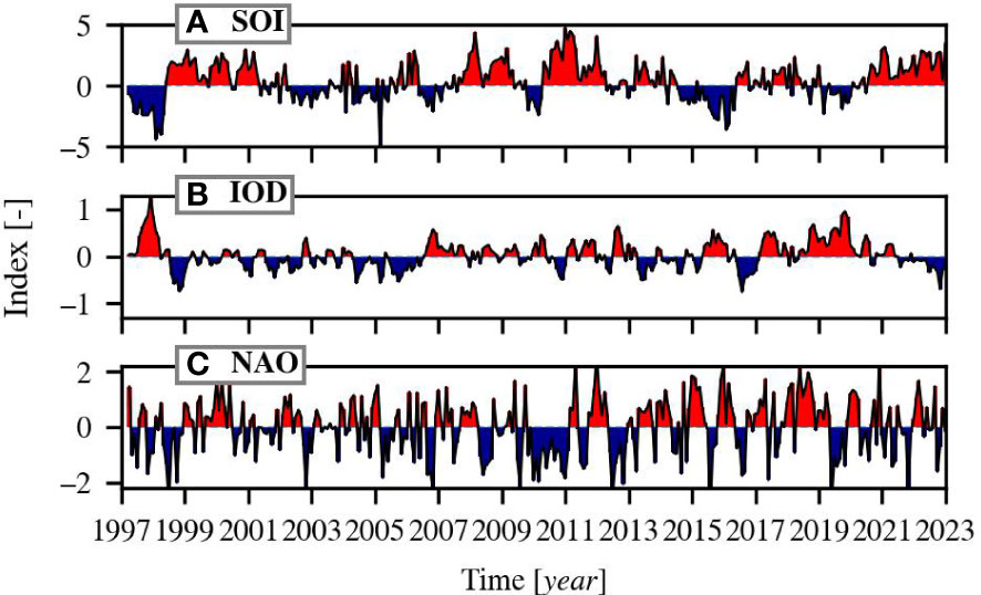
Figure 1 The climate indices of the (A) Southern Oscillation Index (SOI), (B) the Indian Ocean Dipole (IOD) and, (C) North Atlantic Oscillation (NAO). Red indicates positive phases and blue negative phases.

2.4 Longhurst provinces

The global waters were divided into the biogeochemical provinces proposed by Longhurst et al. (1995); Longhurst, 2007). These provinces are defined by distinct physical and biological characteristics, such as mixed layer depth, solar irradiance, and phytoplankton patterns. Each province belongs to one of four different biomes: the polar-, coastal-, trade winds-, or westerly wind biomes.

The 54 Longhurst provinces, each with associated province codes, oceans, and biomes are illustrated in Figure 2 and listed in Table A1 in the Appendix. The shape files of the Longhurst provinces were obtained in April 2022 from the website: https://www.marineregions.org.

FIGURE 2

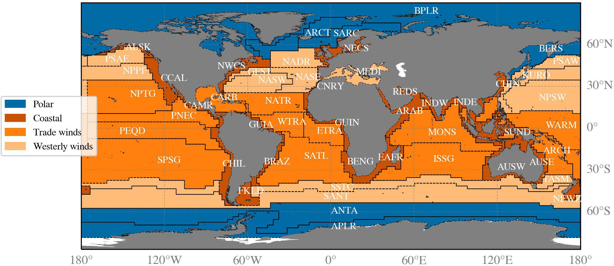
Figure 2 The Longhurst biogeochemical provinces with their four letter acronyms (in white) displayed within the province. The corresponding province descriptions are detailed in Table A1. The colours indicate the four biomes that consist of multiple combined provinces.

2.5 Methods

2.5.1 Temporal gap detection method

First, the global daily OC-CCI data were partitioned into the Longhurst provinces. The Temporal Gap Detection Method (TGDM: Van Oostende et al., 2022) was then applied to each Longhurst province separately. The aim of this method is to filter out unequally observed data over time per geographic pixel and as a result avoids biases in statistics and trends caused by the different spatio-temporal coverage between the sensor input data. Apparent jumps occur in time series of optical properties, when missions join or drop out of the dataset. The main reasons for the inconsistencies within the merged dataset are the different atmospheric corrections, the inconsistent flagging for invalidity between missions, and the overall capabilities of the sensors. Polar-, coastal-, and cloudy regions generally are more affected by these inter-mission inconsistencies. For example, the MERIS sensor has a significantly better coverage of the highly productive shelf waters compared to the SeaWiFS and MODIS sensors. Therefore, when MERIS joins the dataset, much higher values of Chl-a suddenly appear in the global time series. The higher Chl-a values are not incorrect, the only change in the time series is that these type of waters are now included in the dataset. The jumps in the time series should not be confused with natural change, and must be corrected before performing trend analysis.

The TGDM functions as follows: each day within the data of a geographic pixel was scanned for observation availability within a time window of ± n days. If there were no observations for that day or in the time window around it, this day of the year was masked out in every year of that specific geographical pixel. This scanning and filtering is performed on all geographic pixels in the dataset. A time window that is too long may not sufficiently reduce the biased multi-year fluctuations or trends, whereas a time window that is too short results in excessive removal of observations. An optimisation procedure has been applied to find the optimal time window length. This method is proposed and described thoroughly by Van Oostende et al. (2022).

The filtering method used in this manuscript is essentially the same as the TGDM offered by Van Oostende et al. (2022), with some minor adjustments. Firstly, the optimal time window length was determined for each Chl-a time series of the Longhurst provinces separately. Secondly, thresholds of maximum percentage data loss were applied for each biome to ensure that a reasonable number of data records remained available for further analysis. The thresholds used were: trades and westerlies 50%, polar 85%, and coastal 75%. Lastly, this manuscript used version 6 of the OC-CCI dataset, whereas Van Oostende et al. (2022) used version 5. The main differences of the new version, which are of interest for applying the TGDM, are that it has been extended to 2022, includes the OLCI-B sensor, and the active periods of the sensors have been changed. The MODIS and VIIRS sensors have been dropped after 2019 because of data quality concerns due to ageing sensors (Jackson et al., 2022). There are now five, slightly altered broad sub-periods that are used for the optimisation procedure:

1. 9/1997 - 4/2002 only SeaWiFS available

2. 5/2002 - 4/2012 MERIS and MODIS join

3. 5/2012 - 5/2016 VIIRS is launched and MERIS ends

4. 6/2016 - 12/2019 OLCI joins

5. 1/2020 - 6/2022 MODIS and VIIRS end of usage

The Appendix contains a table that shows all optimised time window lengths, and the percentage of data masked per province (Table A2).

Like for the OC-CCI data, the SST-CCI data are merged data from different satellite sensors (Merchant et al., 2019). We expected inconsistency between the missions to be only a secondary effect in the SST data. Both the OC and SST compiling CCI teams already eliminated pure instrumental inter-mission biases. Unlike the analysis of OC data, where the algorithms are affected by the different capabilities in Case-2 or coastal waters compared to the open ocean and thus unevenly flag and discard these pixels that have on the average higher loaded coastal waters, the SST analysis only loses data mainly due to cloud coverage. Nevertheless, we visually inspected the monthly mean time series of each Longhurst region, and since they show no apparent inter-mission bias, we had not applied the TGDM to the SST-CCI data.

2.5.2 Pre-processing of data

Monthly mean composites of Chl-a, K_d490, a_tot443, a_dg443, a_ph443, and b_bp510 were generated by combining all remaining daily records that passed through the TGDM filter. Pixel centres of the ocean colour variables within 4 km from the coastline were excluded due to the larger error associated with these areas, compared to pixels farther from the coastline (Lee et al., 2010). A monthly means composite of the daily sea surface temperature was prepared as well. The salinity data were already a monthly average composite. Monthly average composites of the bias were prepared of the SST, Chl-a, and a_dg443 datasets. These were used for uncertainty estimation and validation of derived trends, i.e. the trend should be larger than the inherent dataset bias. Unfortunately, there was no per-pixel bias available for the salinity data.

All the following statistical- and trend analyses were performed on de-seasonalised, monthly-averaged time series of each ocean colour and climate variable because otherwise the annual cycle would dominate the analyses. De-seasonalisation in this paper always refers to the process of removing the signal caused by seasonality from the time series. These de-seasonalised time series were prepared by decomposing the monthly composites of each variable into a trend-, seasonal- and residual component with Seasonal-Trend decomposition using Loess (STL: Cleveland et al., 1990). The resulting de-seasonalised, monthly-averaged time series consist of the combined trend- and residual components of the decomposed time series.

2.5.3 Statistical- and trend analyses

The statistical relationship between the time series of Chl-a and each optically active constituent was derived globally and for each biome and ocean. The purpose of this correlation analysis was to infer statistical relationships between these optically active constituents and reduce data processing. All ocean colour variables were produced from the same reflectance data, and with high and significant correlation between variables, it is redundant to perform analyses on each product. The ocean colour time series were tested for normality using the Shapiro-Wilk test (Shapiro and Wilk, 1965) to determine the appropriate correlation method. The Spearman correlation method can be applied to non-normally distributed data, whereas the Pearson correlation method is not appropriate in this case. Since approximately one third of the optically active- and climate variables were not normally distributed, all statistical relationships in this study were performed using the Spearman’s rank correlation for the sake of consistency. A significance of at least 95% was used for all correlations. Statistical relationships were also determined between Chl-a and the climate indices and variables to help explain underlying processes.

The non-parametric Mann-Kendall test was used to identify statistically significant trends over time (Mann, 1945; Kendall, 1948). When the resulting τ is not zero and the p-value is greater than 0.95, then the slope of the linear trend was estimated with the non-parametric Sen’s slope (Sen, 1968). This method is insensitive to outliers and has been used in numerous studies that derived trends from ocean colour variables (e.g. Kahru et al., 2011; Frey et al., 2021; Pitarch et al., 2021; Wang et al., 2021). The trend analysis included seasonal and annual Chl-a-, temperature-, salinity trends for each Longhurst province, and Chl-a trends of the different biomes, oceans, and globally.

3 Results

3.1 Statistical relationships between variables

The correlation coefficient between Chl-a and the other investigated optically active constituents is positive globally and in each biome and ocean (Figure 3). The a_dg443 is generally well correlated to Chl-a because Chl-a degradation products are usually the main source of a_dg443 in open waters. The slightly lower correlation between these two variables in the Pacific Ocean, which largely consists of oligotrophic waters, may be due to the delay between the bloom and its breakdown products. These types of waters generally have lower estimation errors for absorption and Chl-a compared to high productive waters (Moore et al., 2009; Lee et al., 2010). The lower correlation between Chl-a and a_dg443 in the coastal biome indicates terrestrial carbon influx. The weaker correlation between a_ph443 and Chl-a may seem counterintuitive as they both are phytoplankton related quantities. However, the relationship between a_ph and Chl-a is variable due to the package effect and pigment composition (Bricaud et al., 1995). The a_ph is associated with larger inaccuracy compared to the other optical variables (Moore et al., 2009; Lee et al., 2010).

FIGURE 3

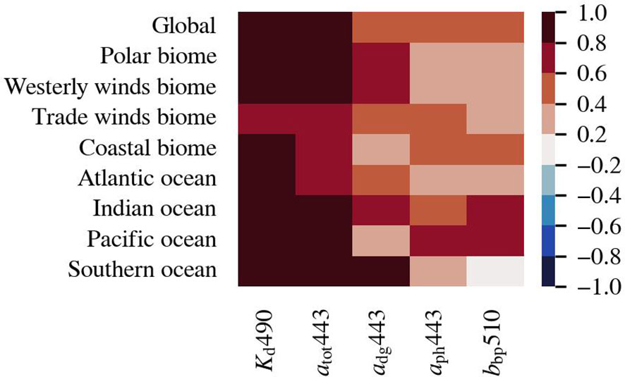
Figure 3 Spearman correlation between de-seasonalised, monthly-averaged time series of Chl-a, and the optically active constituents in the biomes, oceans, and globally (p < 0.005).

Figure 4 demonstrates the correlation between Chl-a and the climate variables and indices. The Chl-a in low latitude-, nutrient-poor provinces are generally negatively correlated to temperature, which implies that increased temperature causes ocean stratification that limits vertical mixing and thus nutrient availability for phytoplankton. The Chl-a in provinces located at higher latitudes that receive limited sunlight, are generally positively correlated with temperature. This could be explained by (a combination of): increased light conditions because of melting ice, increased metabolic rate, and poleward migration of phytoplankton species. Many statistical relationship patterns between Chl-a and salinity are similar to patterns between Chl-a and temperature, but reversed. The positive relationship between Chl-a and salinity in the open ocean provinces can be indirectly attributed to vertical mixing processes related to temperature. Chl-a is generally indirectly related to salinity in coastal provinces, as they are both influenced by interactions between terrestrial runoff, precipitation, and mixing processes. The Chl-a and SOI show the strongest correlation in provinces that are near Tahiti and Darwin (e.g. PEQD and SUND). El Niño phases may restrict phytoplankton growth in or near the pacific equatorial upwelling zones and enhance phytoplankton growth in Southeast Asian- and Australian waters. Thereby, phytoplankton growth enhances in upwelling regions because of enhanced sea level pressure that increases the upwelling nutrient rich waters (Racault et al., 2017). La Niña phases can have the opposite effect. During the time span of this study there have been seven El Niño and seven La Niña phases (Figure 1). The correlation patterns of Chl-a with IOD are quite similar to the correlation patterns between Chl-a and temperature because the IOD is calculated by the difference in sea surface temperature. The NAO phases are linked to westerly wind strength that could either enhance or limit phytoplankton growth through vertical mixing or strat0ification.

FIGURE 4

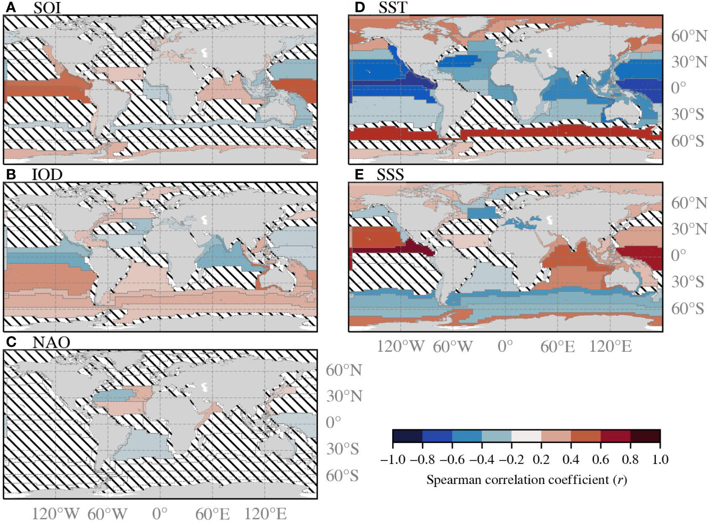
Figure 4 (A–E) Represent the correlation coefficient between the climate variables and the de-seasonalised, monthly-averaged Chl-a time series of each Longhurst province. The correlation coefficient is shown only when the significance is greater than 95%. Slanted lines indicate that the correlation is not significant.

3.2 Trends in the global aquatic ecosystems

Both Figures 5, 6 demonstrate the linear trend direction and magnitude of Chl-a over time. Figure 5 illustrates the time series of Chl-a globally, and in the biomes and oceans, while Figure 6 shows annual and seasonal relative trends of Chl-a, salinity, and temperature in each Longhurst province. The absolute values of trends shown in Figure 6 are available in Table A2 in the Appendix, which also contains information on the averages, standard deviations, and other details for each Longhurst region. The global Chl-a is slightly increasing with 0.002 ± 0.001 mg m^-3 per decade. However, the underlying global uncertainty of the dataset (0.021 mg m^-3) is larger than the global trend. The Chl-a trend direction and magnitude depend heavily on the latitude, as Chl-a increases in most high latitude provinces and decreases in provinces located nearer to the equator. The polar waters experience the greatest increasing Chl-a trends, ranging between 0.027–0.132 ± 0.004–0.03 mg m^-3 per decade. These observations indicate a change in the growth conditions for phytoplankton.

FIGURE 5

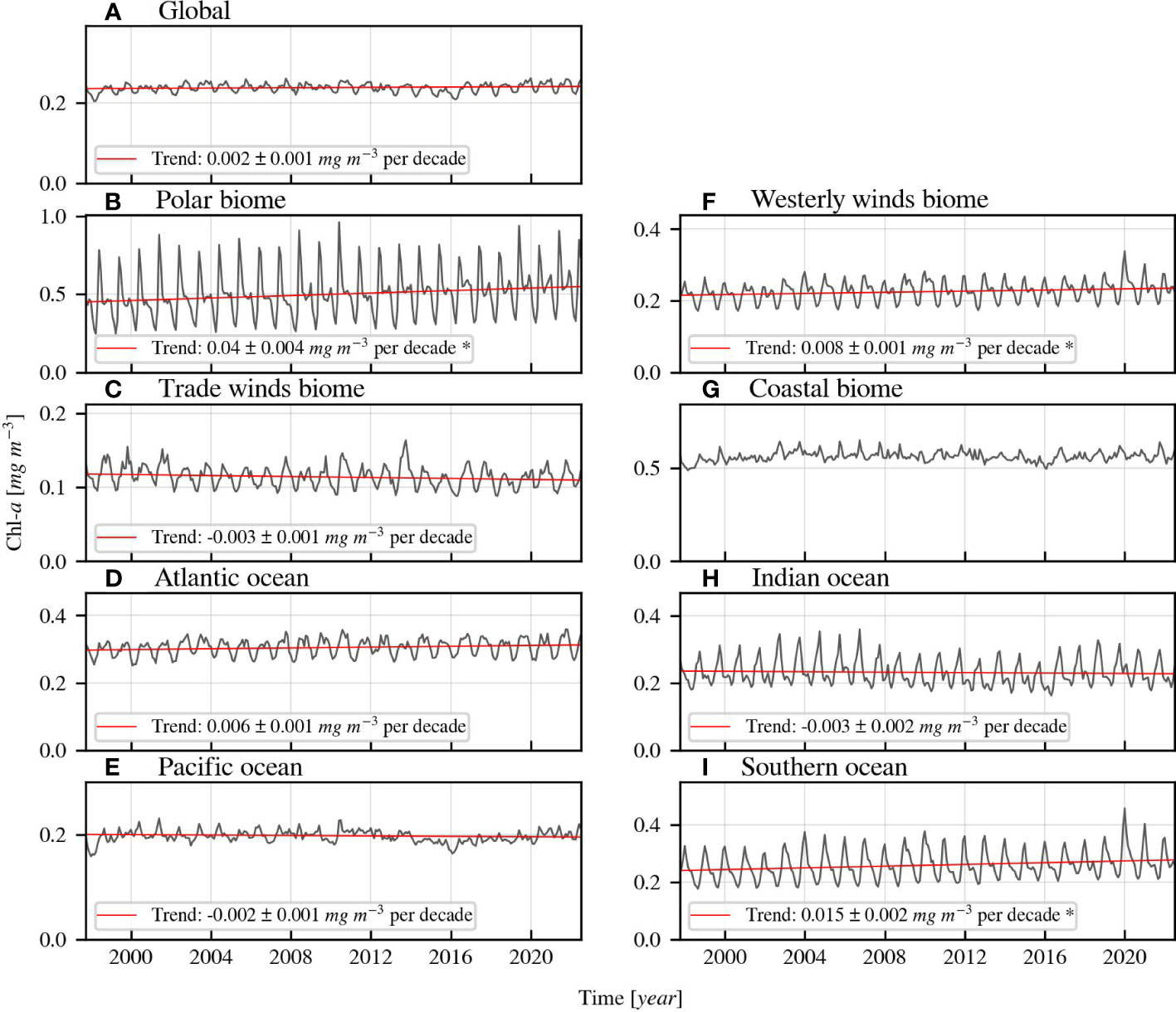
Figure 5 (A–I) Monthly-averaged Chl-a time series of biomes, oceans, and globally with regression lines. The linear regression lines are based on the de-seasonalised (using STL) time series and derived Sen slopes. They are only displayed when the Kendall’s τ indicates significant (>95%) trend. The star (*) behind the formula indicates that the derived trend is larger than the uncertainty of the dataset in the region.

FIGURE 6

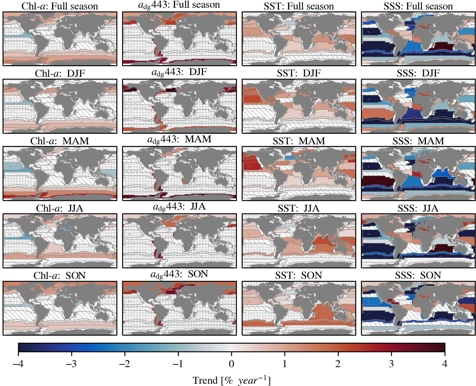
Figure 6 The Sen’s slope of Chl-a, non-phytoplankton absorption at 443 nm (a_dg443), sea surface temperature (SST) and sea surface salinity (SSS) in percent per year. The upper row figures show the trends over a full year and the other rows the trends of specific seasons. Seasons are indicated with a combination of the first letter of the respective month (e.g. December, January, and February = DJF). The trend is only displayed when the Kendall’s τ is significant (>95%). The slanted lines indicate an insignificant τ. The dots indicate provinces where the spatial coverage of the ocean colour variables in the specified season is less than 20% compared to the annual spatial coverage. The trend is not shown when it is smaller than the uncertainty of the underlying province dataset, and is indicated with squares (Appendix: Figure A1). The salinity data did not have any inherent uncertainty information available.

Global warming is evident when looking at the sea surface temperature trends that are increasing in 28 of 54 regions in the range of 0.128–0.477 ± 0.021–0.104 C° per decade. These increasing temperatures affect phytoplankton growth globally. The surface waters of the open ocean are generally freshening, except in the central Atlantic Ocean. The direction of the trend is variable in the coastal provinces. The salinity increased in 20 of 54 provinces with 0.015–0.266 ± 0.006–0.038 PSU per decade and decreased in 25 of 54 provinces with 0.015–0.118 ± 0.003–0.035 PSU per decade. These trends indicate changes in the hydrological cycle, e.g. precipitation and glacier melting, that affect nutrient availability. Additionally, our results suggest that the ocean is darkening, but predominantly in the polar regions, since the non-phytoplankton absorption increased in 13 of 54 provinces, with trends ranging between 0.307–1.164 ± 0.053–0.356 x10² m^-1 per decade. Darkening of waters affect phytoplankton growth by changing the light conditions and is caused by increased decomposition products from marine organisms and increased terrestrial runoff inputs. Coastal waters are usually influenced by terrestrial runoff, whereas open waters are not. The polar waters are typically mentioned with regards to darkening due to increased terrestrial input over time due to climate change (e.g. Konik et al., 2021).

4 Discussion

4.1 Changes in global aquatic ecosystems

We detected trends in optically active constituents over a period of almost 25 years, both globally and in different biogeochemical provinces. This study used time series with improved consistency that is necessary for climate research. All trends discussed here are significant (p<0.05) and are larger than the inherent dataset bias (Appendix: Figure A1), unless otherwise indicated. Our results indicate that global Chl-a is mostly increasing in the polar waters and decreasing in some equatorial waters. The overall global trend is much smaller than the inherent uncertainty of the dataset (0.002 ± 0.001 mg m^-3 per decade < 0.021 mg m^-3), therefore we conclude that there no clear global trend direction of Chl-a. This is in line with findings by Gregg et al. (2017) and Kulk et al. (2020), but contradicts other studies that found a global decreasing trend (Behrenfeld et al., 2006; Boyce et al., 2010; Boyce et al., 2014; Gregg et al., 2014; Hammond et al., 2017), or global increasing trend (Antoine et al., 2005; Hammond et al., 2020). A direct numerical comparison between our results and these studies is impossible because differences can be explained by the use of different time scales, regions, methods, and data sources. Our findings support the conclusions of previous studies that demonstrated that the magnitude and direction of the Chl-a trends vary substantially locally. We observed that Chl-a increased in 22 of 54 regions with 0.011–0.123 ± 0.002–0.026 mg m^-3 per decade and decreased in 6 of 54 regions with 0.012–0.062 ± 0.004–0.019 mg m^-3per decade. Besides changes in phytoplankton dynamics, we indicate that mainly polar waters and some coastal waters are darkening, as the non-phytoplankton absorption increases significantly in these provinces.

Admittedly, the current length of the time series is not long enough yet for definitive conclusions regarding the effect of climate change on phytoplankton dynamics (Henson et al., 2010). It is still important to monitor the state of global waters and response of phytoplankton to a changing environment. The necessary time scale for deriving Chl-a trends is approximately 20–40 years and depends on the region (Henson et al., 2010). With the current time scale, it is possible that we detect trends that are caused by climate indices, e.g. the North Atlantic Oscillation because it has been overwhelmingly positive over the last decade (Figure 1) and may affect Chl-a trends (e.g. Henson et al., 2009; Ferreira et al., 2019; Barbedo et al., 2020).

4.1.1 Polar biome

This study demonstrates a strong increase in Chl-a in all polar provinces coinciding with warming trend of the surface waters. The northernmost province has the highest increase of Chl-a of 0.123 ± 0.026 mg m^-3 per decade. The diminishing ice cover, increased growth rate, and possibly species migration are the likely reason for the positive correlation that we found between Chl-a and temperature (r: 0.2-0.4). The productivity in the polar waters is typically light and temperature dependent (Sakshaug and Slagstad, 1991). Rising temperatures due to global warming lead to decreasing ice cover, which extends the growing season and intensity of phytoplankton blooms as more light is available (Pabi et al., 2008; Ardyna et al., 2014; Arrigo and Van Dijken, 2015; Kahru et al., 2016; Lewis et al., 2020; Frey et al., 2021). Thereby, increasing surface temperatures in polar waters enhances the phytoplankton growth rate and causes northward phytoplankton migration that changes the species composition (Henson et al., 2021).

We observed significant increase of Chl-a in the polar water of the Southern Ocean provinces (0.027–0.093 ± 0.004–0.03 mg m^-3 per decade), consistent with findings of studies by Hammond et al. (2020) and Sathyendranath et al. (2022). The water is freshening in the open waters of the Southern Ocean, likely due to the ice melting. We found a negative relationship between Chl-a and salinity in the open water province of the Southern Ocean (ANTA: r 0.3). In contrast, we found that the surface salinity is increasing near the Antarctic coast, which was also reported by Chaigneau and Morrow (2002) and Kolbe et al. (2021). In the coastal Southern Ocean province the salinity is positively related to Chl-a (APLR: r 0.4), which may be caused by the stronger vertical mixing in these shallower coastal waters and larger brine rejection in the local autumn and winter because of ice cover thinning (Chaigneau and Morrow, 2002; Holland et al., 2006).

In addition to the increase of Chl-a, we also found significant increase of non-phytoplankton absorption in 5 out of 6 polar provinces (not in ANTA). The sources of this increased absorption are increased terrestrial input and/or marine decomposition products. Several studies have found that the dissolved organic carbon in the Arctic Ocean is increasing because of permafrost thawing (Juhls et al., 2019; Mustaffa et al., 2020; Konik et al., 2021; Bernhard et al., 2022). Whereas, Chl-a in the Southern Ocean is highly correlated (r>0.8) with non-phytoplankton absorption, which suggests that the absorption originates from marine decomposition products. This increasing non-phytoplankton absorption leads to darker waters that absorb more light and result in stronger warming of the surface water (Soppa et al., 2019).

4.1.2 Westerly winds biome

In this study, we present evidence that the Chl-a is generally increasing in the westerly wind provinces (6 out of 13), but the increase is not as strong as in the polar provinces (0.011–0.033 mg m^-3 ± 0.002–0.01 mg m^-3 per decade). Interestingly, Chl-a is strongly increasing in the autumn in northern subarctic waters of the Pacific Ocean (PSAE and PSAW: 0.04–0.07 mg m^-3 per decade), which indicates that secondary blooms could be occurring more frequently or have a larger biomass. The Antarctic Circumpolar Current is experiencing strengthening westerly winds (Wang et al., 2011) that possibly increases phytoplankton growth by enhancing vertical mixing in the nutrient-limited Southern Ocean waters (SSTC and SANT: 0.011–0.017 ± 0.002–0.006 mg m^-3 per decade). Climate change can affect the strength of winds in these provinces and thus the mixed layer depth that affects the phytoplankton dynamics, but definitive trends are difficult to derive (for now) because of productivity correlation with natural oscillations, e.g. the El Niño oscillation (Henson et al., 2009). Further research is needed to fully understand the impacts of climate change on phytoplankton dynamics in these dynamic regions.

4.1.3 Trade winds biome

We found decreasing Chl-a trends in the trade wind provinces of the equatorial Pacific and Indian Ocean, in agreement with several studies (Behrenfeld et al., 2006; Hammond et al., 2020; Sathyendranath et al., 2022). However, almost all of these trends are currently smaller than the inherent bias of the dataset. Except for the North Pacific equatorial province (PNEC), which is decreasing with 0.019 ± 0.006 mg m^-3 per decade. This province has a high negative correlation with SST (r: -0.8) and a high positive correlation with salinity (r: 0.8). The negative correlation between Chl-a and surface temperature in these nutrient-limited regions are likely caused by global warming that enhances stratification of the water column and as a result reduces phytoplankton growth rates waters (e.g. Behrenfeld et al., 2006; Boyce et al., 2010; Racault et al., 2012; Lewandowska et al., 2014; Dunstan et al., 2018).

4.1.4 Coastal biome

The coastal provinces are extremely diverse environments that are influenced by land-water exchange processes. Climate change and anthropogenic activities affect numerous regions of this ecosystem (Bindoff et al., 2019). We demonstrated that the Chl-a is changing in many provinces and highlight some of them here.

We observe increasing Chl-a trends in the China Sea (CHIN: 0.019 ± 0.018 mg m^-3 per decade). This is supported by previous research that linked eutrophication of coastal waters to human activities that increase nutrients in the river discharge (Zhou et al., 2020; Wang et al., 2021).

The eastern boundary upwelling systems (BENG, CCAL, CHIL, and CNRY) are highly productive waters defined by continuous cold wind-driven upwelling nutrient-rich water (Kämpf and Chapman, 2016). The upwelling in the Benguela current is forced by global sea-level pressure that is a response to climate change, whereas the upwelling in the other eastern boundary upwelling systems are largely forced by climate oscillations (Bonino et al., 2019). The Chl-a decreases in the Benguela province (BENG: -0.027 ± 0.013 mg m^-3 per decade), which could be explained by decreased upwelling of nutrient-rich water. However, the trend of upwelling is highly dependent on the time period chosen for trend analysis (Bonino et al., 2019).

We show that the Chl-a in the southern coastal provinces of the New Zealand and Eastern Australian shelves is significantly increasing (AUSE and NEWZ: 0.012–0.025 ± 0.003–0.007 mg m^-3 per decade). Our findings are supported by the increasing Chl-a trends found by Kelly et al. (2015), who also reported rapidly increasing salinity and temperature. They argue that the water is more nutrient rich because of increased southerly extension of the East Australian Current and its eddy field. Thompson et al. (2009) reported opposing trends, but used different areas, time scales, and data sources. Additionally, we found relatively high values of Chl-a (and a_dg443) between 2019 and 2021 in the time series of these waters, similar to Tang et al. (2021). They attributed this to the increased forest fires that were caused by enhanced droughts and climate change driven warming.

Many coastal waters in the Indian Ocean are associated with climatic fluctuations of the IOD and SOI (INDW, ARAB, and AUSW: r -0.4-0.4). The strongly seasonal productivity of the western Indian coastal province (INDW) coincides with the monsoon (June-September), whereas productivity in the eastern Indian coastal province (INDE) is less dependent on the monsoon, and is more affected by major river discharges (Longhurst, 2007). Climate change induced glacier melt and increased precipitation in the Ganges and Brahmaputra basins increase peak flow and discharge into the eastern Indian coastal basin during the monsoon (Nepal and Shrestha, 2015). We found that water is freshening in the SON months, which supports their findings. We found an increasing Chl-a trend in the eastern Indian waters (0.014 ± 0.009 mg m^-3 per decade), as opposed to e.g. Behrenfeld et al. (2006) and Gregg et al. (2017). They found that Chl-a declines in both the eastern and western Indian coastal waters. We do indicate a negative Chl-a trend in the western Indian province (-0.054 ± 0.019 mg m^-3 per decade).

4.2 Limitations

The limitation of using TGDM is that daily data records are lost and that seasonality could change since records are filtered depending on the recurrence of observations in every year. An optimised filtering strength (time window) was used to minimise initial data loss and find the optimal reduction of inter-mission inconsistencies per Longhurst province. The strictness, i.e. the length of the time window, and consequently the number of records masked to achieve temporal consistency, differs greatly per province (Appendix: A2A2). This resulted in a slightly larger number of total retained data records of the original dataset, 74%, compared to 70%, when using a universal time window of 27 days for the full OC-CCI v5 dataset (Van Oostende et al., 2022). Data gaps are effectively removed because the use of monthly composites. Another limitation of this study is that some biogeochemical provinces vary significantly optically and biologically and it would be beneficial to separate some of them into smaller provinces. For example, the Mediterranean- and Black Sea should be separated and the Baltic Sea should be separated from the rest of the greater North Sea.

It is important to note that the input SeaWiFS dataset (1997–2010) was atmospherically corrected with l2gen (SeaDAS 7.5; Franz et al., 2007), and the other sensors with POLYMER (v4.1: Steinmetz et al., 2011; Steinmetz et al., 2016). The l2gen processor flags more pixels for invalidity than POLYMER, e.g., observations that consist of high-sensor zenith angels or high values of brightness (Müller et al., 2015). The TGDM circumvents this issue by removing pixels that have not been observed consistently over time (Van Oostende et al., 2022).

There is larger uncertainty associated with optically active constituents retrieved from coastal and polar waters and typically have larger errors compared to other regions (Zheng et al., 2014; IOCCG, 2019; Werdell et al., 2019). Since the Chl-a and a_dg443 are produced by almost the same method (apart from atmospheric correction) and validated extensively with in situ match-ups, we believe it is justified to derive trends in these areas. Thereby, we only show trends that are larger than the inherent uncertainty of the dataset. Unfortunately, uncertainty estimates were not available for the salinity dataset (in our timespan and regions). Due to the limited timescale of the OC-CCI dataset, the bias is currently larger than the trends in most provinces with lower constituent concentrations (e.g. in the trade wind provinces). With future temporal extensions of the dataset, we will likely able to derive trends in these areas.

5 Conclusions

A key challenge in deriving long-term trends from merged ocean colour data is the inconsistency between the spatiotemporal coverage of the input sensor datasets, which can lead to both spurious multi-year fluctuations and trends in the time series. We corrected this inconsistency in the dataset and analysed the derived global and local trends. Our main results demonstrate that global phytoplankton dynamics change in response to different climate feedbacks and indicate a darkening of predominantly polar waters, associated with increasing organic carbon in water. We recommend that future studies that intend to use time series based on merged satellite datasets consider whether their data are affected by inter-mission coverage inconsistencies and, if necessary, apply a method to minimise these. Additionally, previous studies that used time series based on merged ocean colour datasets may benefit from re-evaluating their findings. Future research should further investigate global and local trends in optically active constituents, especially when these time series become long enough to draw definitive conclusions on the effects of climate change on global waters and phytoplankton dynamics.

Data availability statement

Publicly available datasets were analyzed in this study. This data can be found here: https://www.oceancolour.org/ https://climate.esa.int/en/projects/sea-surface-temperature/ https://cds.climate.copernicus.eu/cdsapp#!/dataset/reanalysis-oras5?tab=form.

Author contributions

All authors jointly developed the concept and work plan. MO performed the calculations, preparated the figures, had lead on writing the manuscript. All authors contributed to the article and approved the submitted version.

Acknowledgments

This work is a contribution to the Ocean Colour Climate Change Initiative of the European Space Agency and was supported by the Helmholtz Association within the Earth and Environment research program. We thank Rüdiger Röttgers, Michael Novak, Sjoerd Koopman, and the reviewers for their valuable commentary.

Conflict of interest

The authors declare that the research was conducted in the absence of any commercial or financial relationships that could be construed as a potential conflict of interest.

Publisher’s note

All claims expressed in this article are solely those of the authors and do not necessarily represent those of their affiliated organizations, or those of the publisher, the editors and the reviewers. Any product that may be evaluated in this article, or claim that may be made by its manufacturer, is not guaranteed or endorsed by the publisher.

Supplementary material

The Supplementary Material for this article can be found online at: https://www.frontiersin.org/articles/10.3389/fmars.2023.1052166/full#supplementary-material

References

Antoine D., Morel A., Gordon H. R., Banzon V. F., Evans R. H. (2005). Bridging ocean color observations of the 1980s and 2000s in search of long-term trends. J. Geophys. Res. Ocean. 110, 1–22. doi: 10.1029/2004JC002620

CrossRef Full Text | Google Scholar

Ardyna M., Arrigo K. R. (2020). Phytoplankton dynamics in a changing Arctic ocean. Nat. Clim. Change 10, 892–903. doi: 10.1038/s41558-020-0905-y

CrossRef Full Text | Google Scholar

Ardyna M., Babin M., Gosselin M., Devred E., Rainville L., Tremblay J. E. (2014). Fall phytoplankton blooms. Geophys. Res. Lett. 41, 6207–6212. doi: 10.1002/2014GL061047

CrossRef Full Text | Google Scholar

Arrigo K. R., Van Dijken G. L. (2015). Continued increases in Arctic ocean primary production. Prog. Oceanogr. 136, 60–70. doi: 10.1016/J.POCEAN.2015.05.002

CrossRef Full Text | Google Scholar

Barbedo L., Bélanger S., Tremblay J.É. (2020). Climate control of sea-ice edge phytoplankton blooms in the Hudson bay system. Elementa 8, 1–25. doi: 10.1525/elementa.039

CrossRef Full Text | Google Scholar

Behrenfeld M. J., O’Malley R. T., Siegel D. A., McClain C. R., Sarmiento J. L., Feldman G. C., et al. (2006). Climate-driven trends in contemporary ocean productivity. Nature 444, 752–755. doi: 10.1038/nature05317

PubMed Abstract | CrossRef Full Text | Google Scholar

Bernhard P., Zwieback S., Hajnsek I. (2022). Accelerated mobilization of organic carbon from retrogressive thaw slumps on the northern taymyr peninsula. Cryosphere 16, 2819–2835. doi: 10.5194/TC-16-2819-2022

CrossRef Full Text | Google Scholar

Bidigare R. R., Ondrusek M. E., Brooks J. M. (1993). Influence of the Orinoco river outflow on distributions of algal pigments in the Caribbean Sea. J. Geophys. Res. 98, 2259–2269. doi: 10.1029/92JC02762

CrossRef Full Text | Google Scholar

Bindoff N. L., Cheung W. W. L., Kairo J. G., Arístegui J., Guinder V. A., Hallberg R., et al. (2019). “Changing ocean, marine ecosystems, and dependent communities,” in IPCC special report on the ocean and cryosphere in a changing climate. Eds. Pörtner H.-O., Roberts D. C., Masson-Delmotte V., Zhai P., Tignor M., Poloczanska E., et al (Cambridge, UK and New York, NY, USA: Cambridge University Press), 447–587. doi: 10.1017/9781009157964.007

CrossRef Full Text | Google Scholar

Bonino G., Di Lorenzo E., Masina S., Iovino D. (2019). Interannual to decadal variability within and across the major Eastern boundary upwelling systems. Sci. Rep. 9, 1–14. doi: 10.1038/s41598-019-56514-8

PubMed Abstract | CrossRef Full Text | Google Scholar

Boyce D. G., Dowd M., Lewis M. R., Worm B. (2014). Estimating global chlorophyll changes over the past century. Prog. Oceanogr. 122, 163–173. doi: 10.1016/j.pocean.2014.01.004

CrossRef Full Text | Google Scholar

Boyce D. G., Lewis M. R., Worm B. (2010). Global phytoplankton decline over the past century. Nature 466, 591–596. doi: 10.1038/nature09268

PubMed Abstract | CrossRef Full Text | Google Scholar

Bricaud A., Babin M., Morel A., Claustre H. (1995). Variability in the chlorophyll-specific absorption coefficients of natural phytoplankton: analysis and parameterization. JGR Oceans 100(C7), 13321–13332. doi: 10.1029/95JC00463

CrossRef Full Text | Google Scholar

Brown J. H., Gillooly J. F., Allen A. P., Savage V. M., West G. B. (2004). Toward a metabolic theory of ecology. Ecology 85, 1771–1789. doi: 10.1890/03-9000

CrossRef Full Text | Google Scholar

Burke L. A., Kura Y., Kassem K., Revenga C., Spalding M., McAllister D. (2001). Pilot Analysis of Global Ecosystems: Coastal Ecosystems. Washington, DC: World Resources Institute, p. 77

Google Scholar

Chaigneau A., Morrow R. (2002). Surface temperature and salinity variations between Tasmania and Antarctica 1993-1999. J. Geophys. Res. 107 (C12), SRF 22-1–SRF 22-8. doi: 10.1029/2001JC000808

CrossRef Full Text | Google Scholar

Cleveland R. B., Cleveland W. S., McRae J. E., Terpenning I. (1990). STL: a seasonal-trend decomposition procedure based on loess. J. Off. Stat. 6, 3–73. doi: 10.1007/978-1-4613-4499-5_24

CrossRef Full Text | Google Scholar

Cullen J. J. (1982). The deep chlorophyll maximum: comparing vertial profiles of chlorophyll a. Can. J. Fish. Aquat. Sci. 39, 791–803. doi: 10.1139/f82-108

CrossRef Full Text | Google Scholar

Deppeler S. L., Davidson A. T. (2017). Southern ocean phytoplankton in a changing climate. Front. Mar. Sci. 4. doi: 10.3389/fmars.2017.00040

CrossRef Full Text | Google Scholar

Dunstan P. K., Foster S. D., King E., Risbey J., Kane T. J. O., Monselesan D., et al. (2018). Global patterns of change and variation in sea surface temperature and chlorophyll a. Scientific Reports 8, 14624. doi: 10.1038/s41598-018-33057-y

CrossRef Full Text | Google Scholar

Durack P. J., Wijffels S. E. (2010). Fifty-year trends in global ocean salinities and their relationship to broad-scale warming. J. Clim. 23, 4342–4362. doi: 10.1175/2010JCLI3377.1

CrossRef Full Text | Google Scholar

Ferreira A., Garrido-Amador P., Brito A. C. (2019). Disentangling environmental drivers of phytoplankton biomass off Western Iberia. Front. Mar. Sci. 6. doi: 10.3389/FMARS.2019.00044/FULL

CrossRef Full Text | Google Scholar

Franz B. A., Bailey S. W., Werdell P. J., Mcclain C. R. (2007). Sensor-independent approach to the vicarious calibration of satellite ocean color radiometry. Appl. Opt. 46, 5068–5082. doi: 10.1364/AO.46.005068

PubMed Abstract | CrossRef Full Text | Google Scholar

Frey K. E., Comiso J. C., Cooper L. W., Grebmeier J. M., Stock L. V. (2021). "Arctic Ocean primary productivity: the response of marine algae to climate warming and Sea ice decline" in. Arctic Report Card. Eds., Moon T. A., Druckenmiller M. L., Thoman R. L., doi: 10.25923/kxhb-dw16

CrossRef Full Text | Google Scholar

Friedland K. D., Mouw C. B., Asch R. G., Ferreira A. S. A., Henson S., Hyde K. J. W., et al. (2018). Phenology and time series trends of the dominant seasonal phytoplankton bloom across global scales. Glob. Ecol. Biogeogr. 27, 551–569. doi: 10.1111/geb.12717

CrossRef Full Text | Google Scholar

Gattuso J. P., Magnan A., Billé R., Cheung W. W. L., Howes E. L., Joos F., et al. (2015). Contrasting futures for ocean and society from different anthropogenic CO2 emissions scenarios. Science 349 (6243), aac4722. doi: 10.1126/science.aac4722

PubMed Abstract | CrossRef Full Text | Google Scholar

GCOS. (2011). Systematic observation requirements for satellite-based products for climate. Available at: www.wmo.int/pages/prog/gcos/Publications/gcos-154.pdf.

Google Scholar

GCOS (2016). The global observing system for climate: implementation needs. Available at: https://library.wmo.int/doc_num.php?explnum_id=3417.

Google Scholar

Good S. A., Embury O., Bulgin C. E., Mittaz J. (2019). ESA Sea Surface temperature climate change initiative (SST_cci): level 4 analysis climate data record, version 2.1. doi: 10.5285/aced40d7cb964f23a0fd3e85772f2d48

CrossRef Full Text | Google Scholar

Gregg W. W., Ecile C., Rousseaux S. (2014). Decadal trends in global pelagic ocean chlorophyll: a new assessment integrating multiple satellites, in situ data, and models. J. Geophys. Res. Ocean. 119, 5921–5933. doi: 10.1002/2014JC010158

CrossRef Full Text | Google Scholar

Gregg W. W., Rousseaux C. S., Franz B. A. (2017). Global trends in ocean phytoplankton: a new assessment using revised ocean colour data. Remote Sens Lett. 8 (8), 1102–1111. doi: 10.1080/2150704X.2017.1354263

PubMed Abstract | CrossRef Full Text | Google Scholar

Hammond M. L., Beaulieu C., Henson S. A., Sahu S. K. (2020). Regional surface chlorophyll trends and uncertainties in the global ocean. Sci. Rep. 10 (1), 15273. doi: 10.1038/s41598-020-72073-9

PubMed Abstract | CrossRef Full Text | Google Scholar

Hammond M. L., Beaulieu C., Sahu S. K., Henson S. A. (2017). Assessing trends and uncertainties in satellite-era ocean chlorophyll using space-time modeling. Global Biogeochem. Cycles 31, 1103–1117. doi: 10.1002/2016GB005600

CrossRef Full Text | Google Scholar

Henson S. A., Cael B. B., Allen S. R., Dutkiewicz S. (2021). Future phytoplankton diversity in a changing climate. Nat. Commun. 12, 5372. doi: 10.1038/s41467-021-25699-w

PubMed Abstract | CrossRef Full Text | Google Scholar

Henson S. A., Dunne J. P., Sarmiento J. L. (2009). Decadal variability in north Atlantic phytoplankton blooms. J. Geophys. Res. Ocean. 114, C04013. doi: 10.1029/2008JC005139

CrossRef Full Text | Google Scholar

Henson S. A., Sarmiento J. L., Dunne J. P., Bopp L., Lima I., Doney S. C., et al. (2010). Detection of anthropogenic climate change in satellite records of ocean chlorophyll and productivity. Biogeosciences 7, 621–640. doi: 10.5194/bg-7-621-2010

CrossRef Full Text | Google Scholar

Holland M. M., Bitz C. M., Tremblay B. (2006). Future abrupt reductions in the summer Arctic sea ice future abrupt reductions in the summer Arctic sea ice. Geophys. Res. Lett. 33, L23503. doi: 10.1029/2006GL028024

CrossRef Full Text | Google Scholar

Hurrell J. W., Kushnir Y., Ottersen G., Visbeck M. (2003). An overview of the north atlantic oscillation. Geophys. Monogr. Ser. 134, 1–35. doi: 10.1029/134GM01

CrossRef Full Text | Google Scholar

IOCCG. (2019). Uncertainties in ocean colour remote sensing. no. 18. Ed. Mélin Dartmouth F. (Canada: International Ocean-Colour Coordinating Group). doi: 10.25607/OBP-696

CrossRef Full Text | Google Scholar

Jackson T., Sathyendranath S., Groom S., Calton B. (2022) Product user guide for v6.0 dataset. D4.2. ocean colour climate change initiative (OC_CCI) – phase 3. Available at: https://docs.pml.space/share/s/fzNSPb4aQaSDvO7xBNOCIw.

Google Scholar

Jackson T., Volpe G., Sathyendranath S., Groom S. (2021). Product validation and intercomparison report (Plymouth). (Plymouth Marine Laboratory (PML) and ESA Climate Office) (https://climate.esa.int). Available at: https://docs.pml.space/share/s/xztLpMNRka9rqoeSQFw5A

Google Scholar

Joseph D., Rojith G., Zacharia P. U., Sajna V. H., Akash S., George G. (2021). Spatio-temporal variations of chlorophyll from satellite derived data and CMIP5 models along Indian coastal regions. J. Earth Syst. Sci. 130, 1–12. doi: 10.1007/s12040-021-01663-6

CrossRef Full Text | Google Scholar

Juhls B., Overduin P. P., Hölemann J., Hieronymi M., Matsuoka A., Heim B., et al. (2019). Dissolved organic matter at the fluvial-marine transition in the laptev Sea using in situ data and ocean colour remote sensing. Biogeosciences 16, 2693–2713. doi: 10.5194/BG-16-2693-2019

CrossRef Full Text | Google Scholar

Kahru M., Brotas V., Manzano-Sarabia M., Mitchell B. G. (2011). Are phytoplankton blooms occurring earlier in the Arctic? Glob. Change Biol. 17, 1733–1739. doi: 10.1111/j.1365-2486.2010.02312.x

CrossRef Full Text | Google Scholar

Kahru M., Kudela R. M., Manzano-Sarabia M., Greg Mitchell B. (2012). Trends in the surface chlorophyll of the California current: merging data from multiple ocean color satellites. Deep. Res. Part II Top. Stud. Oceanogr. 77–80, 89–98. doi: 10.1016/j.dsr2.2012.04.007

CrossRef Full Text | Google Scholar

Kahru M., Lee Z. P., Kudela R. M., Manzano-Sarabia M., Greg Mitchell B. (2015). Multi-satellite time series of inherent optical properties in the California current. Deep. Res. Part II Top. Stud. Oceanogr. 112, 91–106. doi: 10.1016/j.dsr2.2013.07.023

CrossRef Full Text | Google Scholar

Kahru M., Lee Z., Mitchell B. G., Nevison C. D. (2016). Effects of sea ice cover on satellite- detected primary production in the Arctic ocean. Arct. Ocean. Biol. Lett. 12. doi: 10.1098/rsbl.2016.0223

CrossRef Full Text | Google Scholar

Kämpf J., Chapman P. (2016). "The functioning of coastal upwelling systems". In: Upwelling Systems of the World., (Springer, Cham) p. 31–65. doi: 10.1007/978-3-319-42524-5_2

CrossRef Full Text | Google Scholar

Kelly P., Clementson L., Lyne V. (2015). Decadal and seasonal changes in temperature, salinity, nitrate, and chlorophyll in inshore and offshore waters along southeast Australia. J. Geophys. Res. Ocean. 120, 4226–4244. doi: 10.1002/2014JC010485

CrossRef Full Text | Google Scholar

Kendall M. G. (1948). Rank Correlation Methods. [Pp. vii 160. London: Charles Griffin and Co. Ltd., 42 Drury Lane, 18s.]. Journal of the Institute of Actuaries. 75 (1), 140–141. doi: 10.1017/S0020268100013019

Google Scholar

Kirk J. T. O. (2011). Light and photosynthesis in aquatic ecosystems. 3rd ed (Cambridge, UK: Cambridge University Press). doi: 10.1017/CBO9781139168212

CrossRef Full Text | Google Scholar

Kolbe M., Roquet F., Pauthenet E., Nerini D. (2021). Impact of thermohaline variability on Sea level changes in the southern ocean. J. Geophys. Res. Ocean. 126 (9), e2021JC017381. doi: 10.1029/2021JC017381

CrossRef Full Text | Google Scholar

Konik M., Darecki M., Pavlov A. K., Sagan S., Kowalczuk P. (2021). Darkening of the Svalbard fjords waters observed with satellite ocean color imagery in 1997–2019. Front. Mar. Sci. 8. doi: 10.3389/fmars.2021.699318

CrossRef Full Text | Google Scholar

Kulk G., Platt T., Dingle J., Jackson T., Jönsson B. F., Bouman H. A., et al. (2020). Primary production, an index of climate change in the ocean: satellite-based estimates over two decades. Remote Sens. 12, 1–27. doi: 10.3390/rs12050826

CrossRef Full Text | Google Scholar

Lee Z. P., Arnone R., Hu C., Werdell P. J., Lubac B. (2010). Uncertainties of optical parameters and their propagations in an analytical ocean color inversion algorithm. Appl. Opt. 49, 369–381. doi: 10.1364/AO.49.000369

PubMed Abstract | CrossRef Full Text | Google Scholar

Lee Z. P., Darecki M., Carder K. L., Davis C. O., Stramski D., Rhea W. J. (2005). Diffuse attenuation coefficient of downwelling irradiance: an evaluation of remote sensing methods. J. Geophys. Res. C Ocean. 110, 1–9. doi: 10.1029/2004JC002573

CrossRef Full Text | Google Scholar

Lee Z. P., Lubac B., Werdell J., Arnone R. (2009) An update of the quasi-analytical algorithm (QAA_v5). tech. report, int. ocean colour coord. gr. Available at: http://www.ioccg.org/groups/software.html.

Google Scholar

Lewandowska A. M., Boyce D. G., Hofmann M., Matthiessen B., Sommer U., Worm B. (2014). Effects of sea surface warming on marine plankton. Ecol. Lett. 17, 614–623. doi: 10.1111/ele.12265

PubMed Abstract | CrossRef Full Text | Google Scholar

Lewis K. M., Van Dijken G. L., Arrigo K. R. (2020). Changes in phytoplankton concentration now drive increased Arctic ocean primary production. Sci. (80-. ). 369, 198–202. doi: 10.1126/science.aay8380

CrossRef Full Text | Google Scholar

Longhurst A. R. (2007). Ecological geography of the Sea. 2nd ed (London: Academic Press). doi: 10.1016/B978-0-12-455521-1.X5000-1

CrossRef Full Text | Google Scholar

Longhurst A., Sathyendranath S., Platt T., Caverhill C. (1995). An estimate of global primary production in the ocean from satellite radiometer data. J. Plankton Res. 17, 1245–1271. doi: 10.1093/PLANKT/17.6.1245

CrossRef Full Text | Google Scholar

Mann H. B. (1945). Nonparametric tests against trend. Econometrica 13, 245. doi: 10.2307/1907187

CrossRef Full Text | Google Scholar

Merchant C. J., Embury O., Bulgin C. E., Block T., Corlett G. K., Fiedler E., et al. (2019). Satellite-based time-series of sea- surface temperature since 1981 for climate applications. Sci. Data 6, 223. doi: 10.1038/s41597-019-0236-x

PubMed Abstract | CrossRef Full Text | Google Scholar

Moore T. S., Campbell J. W., Dowell M. D. (2009). A class-based approach to characterizing and mapping the uncertainty of the MODIS ocean chlorophyll product. Remote Sens. Environ. 113, 2424–2430. doi: 10.1016/j.rse.2009.07.016

CrossRef Full Text | Google Scholar

Morel A. A., Prieur L. (1977). Analysis of variations in ocean color. Limnol. Oceanogr. 22, 709–722. doi: 10.4319/LO.1977.22.4.0709

CrossRef Full Text | Google Scholar

Müller D., Krasemann H., Brewin R. J. W., Brockmann C., Deschamps P. Y., Doerffer R., et al. (2015). The ocean colour climate change initiative: i. a methodology for assessing atmospheric correction processors based on in-situ measurements. Remote Sens. Environ. 162, 242–256. doi: 10.1016/j.rse.2013.11.026

CrossRef Full Text | Google Scholar

Mustaffa N. I. H., Kallajoki L., Biederbick J., Binder F. I., Schlenker A., Striebel M. (2020). Coastal ocean darkening effects via terrigenous DOM addition on plankton: an indoor mesocosm experiment. Front. Mar. Sci. 7. doi: 10.3389/fmars.2020.547829

CrossRef Full Text | Google Scholar

Navarro G., Almaraz P., Caballero I., Vázquez Á., Huertas I. E. (2017). Reproduction of spatio-temporal patterns of major mediterranean phytoplankton groups from remote sensing OC-CCI data. Front. Mar. Sci. 4. doi: 10.3389/fmars.2017.00246

CrossRef Full Text | Google Scholar

Nepal S., Shrestha A. B. (2015). Impact of climate change on the hydrological regime of the indus, Ganges and Brahmaputra river basins: a review of the literature. Int. J. Water Resour. Dev. 31, 201–218. doi: 10.1080/07900627.2015.1030494

CrossRef Full Text | Google Scholar

O’Gorman P. A. (2015). Precipitation extremes under climate change. Curr. Clim. Change Rep. 1, 49–59. doi: 10.1007/s40641-015-0009-3

PubMed Abstract | CrossRef Full Text | Google Scholar

Pabi S., Van Dijken G. L., Arrigo K. R. (2008). Primary production in the Arctic ocean 1998-2006. J. Geophys. Res. Ocean. 113, 1998–2006. doi: 10.1029/2007JC004578

CrossRef Full Text | Google Scholar

Pitarch J., Bellacicco M., Marullo S., van der Woerd H. J. (2021). Global maps of forel-ule index, hue angle and secchi disk depth derived from twenty-one years of monthly ESA-OC-CCI data. Earth Syst. Sci. Data 13, 481–490. doi: 10.5194/essd-13-481-2021

CrossRef Full Text | Google Scholar

Racault M. F., Le Quéré C., Buitenhuis E., Sathyendranath S., Platt T. (2012). Phytoplankton phenology in the global ocean. Ecol. Indic. 14, 152–163. doi: 10.1016/j.ecolind.2011.07.010

CrossRef Full Text | Google Scholar

Racault M., Sathyendranath S., Brewin R. J. W. (2017). Impact of El niño variability on oceanic phytoplankton. Front. Mar. Sci. 4, 133. doi: 10.3389/fmars.2017.00133

CrossRef Full Text | Google Scholar

Saji N. H., Yamagata T. (2003). Possible impacts of Indian ocean dipole mode events on global climate. Clim. Res. 25, 151–169. doi: 10.3354/cr025151

CrossRef Full Text | Google Scholar

Sakshaug E., Slagstad D. (1991). Light and productivity of phytoplankton in polar marine ecosystems: a physiological view. Polar Res. 10, 69–86. doi: 10.3402/POLAR.V10I1.6729

CrossRef Full Text | Google Scholar

Sankar S., Thondithala Ramachandran A., Franck Eitel K. G., Kondrik D., Sen R., Madipally R., et al. (2019). The influence of tropical Indian ocean warming and Indian ocean dipole on the surface chlorophyll concentration in the eastern Arabian Sea. Biogeosciences Discuss., 1–23. doi: 10.5194/bg-2019-169

CrossRef Full Text | Google Scholar

Sathyendranath S., Brewin R. J. W. W., Brockmann C., Brotas V., Calton B., Chuprin A., et al. (2019). An ocean-colour time series for use in climate Studies : the experience of the ocean-colour climate (OC-CCI). Sensors 19, 2–31. doi: 10.3390/s19194285

CrossRef Full Text | Google Scholar

Sathyendranath S., Groom S. B., Jackson T., Volpe G., Calton B. (2022) ESA Ocean colour climate change initiative-phase 3 climate assessment report. Available at: https://docs.pml.space/share/s/vS7lSM2DRBqrM9APK-PJkw.

Google Scholar

Sen P. K. (1968). Estimates of the regression coefficient based on kendall’s tau. J. Am. Stat. Assoc. 63, 1379–1389. doi: 10.1080/01621459.1968.10480934

CrossRef Full Text | Google Scholar

Shapiro S. S., Wilk M. B. (1965). Biometrika trust an analysis of variance test for normality (Complete samples). Source: Biometrika 52, 591–611. doi: 10.2307/2333709

CrossRef Full Text | Google Scholar

Soppa M. A., Pefanis V., Hellmann S., Losa S. N., Hölemann J., Martynov F., et al. (2019). Assessing the influence of water constituents on the radiative heating of laptev Sea shelf waters. Front. Mar. Sci. 6, 221. doi: 10.3389/fmars.2019.00221

CrossRef Full Text | Google Scholar

Steinmetz F., Deschamps P.-Y., Ramon D. (2011). Atmospheric correction in presence of sun glint: application to MERIS. Opt. Express 19, 9783. doi: 10.1364/oe.19.009783

PubMed Abstract | CrossRef Full Text | Google Scholar

Steinmetz F., Ramon D., Deschamps P.-Y. (2016) ATBD v1 - polymer atmospheric correction algorithm. Available at: https://docs.pml.space/share/s/M05k8Lw3QLeXSIiA3X87UQ.

Google Scholar

Tang W., Llort J., Weis J., G Perron M. M., Basart S., Li Z., et al. (2021). Widespread phytoplankton blooms triggered by 2019-2020 Australian wildfires. Nature 597, 370–375. doi: 10.1038/s41586-021-03805-8

PubMed Abstract | CrossRef Full Text | Google Scholar

Thompson P. A., Baird M. E., Ingleton T., Doblin M. A. (2009). Long-term changes in temperate Australian coastal waters: implications for phytoplankton. Mar. Ecol. Prog. Ser. 394, 1–19. doi: 10.3354/meps08297

CrossRef Full Text | Google Scholar

Valente A., Sathyendranath S., Brotas V., Groom S., Grant M., Taberner M., et al. (2019). A compilation of global bio-optical in situ data for ocean-colour satellite applications - version two. Copernicus Publications: Earth System Science Data 11 (3), 1037–1068. doi: 10.5194/essd-11-1037-2019

CrossRef Full Text | Google Scholar

Van Oostende M., Hieronymi M., Krasemann H., Baschek B., Röttgers R. (2022). Correction of inter-mission inconsistencies in merged ocean colour satellite data. Front. Remote Sens. 3, 1–17. doi: 10.3389/frsen.2022.882418

CrossRef Full Text | Google Scholar

Wang W., Anderson B. T., Kaufmann R. K., Myneni R. B. (2004). The relation between the north Atlantic oscillation and SSTs in the north Atlantic basin. J. Clim. 17, 4752–4759. doi: 10.1175/JCLI-3186.1

CrossRef Full Text | Google Scholar

Wang Z., Kuhlbrodt T., Meredith M. P. (2011). On the response of the Antarctic circumpolar current transport to climate change in coupled climate models. J. Geophys. Res. Ocean. 116, 1–17. doi: 10.1029/2010JC006757

CrossRef Full Text | Google Scholar

Wang Y., Tian X., Gao Z. (2021). Evolution of satellite derived chlorophyll-a trends in the bohai and yellow seas during 2002–2018: comparison between linear and nonlinear trends. Estuar. Coast. Shelf Sci. 259, 107449. doi: 10.1016/J.ECSS.2021.107449

CrossRef Full Text | Google Scholar

Wells M. L., Karlson B., Wulff A., Kudela R., Trick C., Asnaghi V., et al. (2020). Future HAB science: directions and challenges in a changing climate. Harmful Algae 91, 101632. doi: 10.1016/j.hal.2019.101632

PubMed Abstract | CrossRef Full Text | Google Scholar

Werdell P. J., Mckinna L. I. W., Boss E., Ackleson S. G., Craig S. E., Gregg W. W., et al. (2019). An overview of approaches and challenges for retrieving marine inherent optical properties from ocean color remote sensing. Prog. Oceanogr. 160, 186–212. doi: 10.1016/j.pocean.2018.01.001

CrossRef Full Text | Google Scholar

Wirtz K., Smith S. L., Mathis M., Taucher J. (2022). Vertically migrating phytoplankton fuel high oceanic primary production. Nat. Clim. Change 12, 750–756. doi: 10.1038/s41558-022-01430-5

CrossRef Full Text | Google Scholar

Zheng G., Stramski D., Reynolds R. A. (2014). Evaluation of the quasi-analytical algorithm for estimating the inherent optical properties of seawater from ocean color: comparison of Arctic and lower-latitude waters. Remote Sens. Environ. 155, 194–209. doi: 10.1016/j.rse.2014.08.020

CrossRef Full Text | Google Scholar

Zhou Y., Wang L., Zhou Y., Mao X.z. (2020). Eutrophication control strategies for highly anthropogenic influenced coastal waters. Sci. Total Environ. 705, 135760. doi: 10.1016/J.SCITOTENV.2019.135760

PubMed Abstract | CrossRef Full Text | Google Scholar

Zuo H., Balmaseda M. A., Mogensen K., Tietsche S. (2018). OCEAN5: the ECMWF ocean reanalysis system and its real-time analysis component. ECMWF Technical Memoranda, No. 823. doi: 10.21957/la2v0442

CrossRef Full Text | Google Scholar