Variations of phytoplankton chlorophyll in the Bay of Bengal: Impact of climate changes and nutrients from different sources

1 Introduction

The Bay of Bengal (BoB), among the largest of the Large Marine Ecosystems (LMEs) in the world, is bounded by the Asian continent in the north, the eastern coast of India in the west, and the Andaman Sea in the east. In the south, the bay is open to the Indian Ocean. The surrounding countries of India, Bangladesh, Sri Lanka, Myanmar, the Maldives, Thailand, Malaysia, and Indonesia have reached a consensus on a strategic action program to solve existing socioeconomic issues (e.g., Elayaperumal et al., 2019) because of the social and economic importance of the bay.

One of the key determinants of the services the BoB provides to nearby societies and economies is phytoplankton primary production, a common metric of which is phytoplankton biomass or chlorophyll-a concentration (CHL, mg m⁻³). Primary production is the production of organic matter at the base of the marine food web and supports the secondary production of biomass by marine organisms at higher trophic levels. Previous studies have reported a strong relationship between CHL, or primary production, and fisheries production in a wide variety of marine ecosystems in coastal waters and the open ocean (Nixon and Thomas, 2001; Nixon and Buckley, 2002). The production of the tropical Hilsa fishery, which contributes to the society and economy of India, Bangladesh, and Myanmar, is controlled by primary production in the BoB (Hossain et al., 2020).

Light, in addition to nutrients, is an important determinant of primary production in the BoB, especially in the northern part of the bay because of the high turbidity associated with high sediment inputs from the Ganges and Brahmaputra Rivers (GBR) (Kumar et al., 2010). Because of the large influx of freshwater from the GBR, the water column in the northern BoB is strongly stratified. This stratification inhibits the influx of inorganic nutrients from the ocean subsurface layer to the euphotic zone, especially in the central part of the bay and during boreal summer (Kumar et al., 2002). In the part of the bay where light is not a limiting factor, the input of inorganic nutrients is thought to be the major determinant of primary production in the BoB.

There are at least three major sources of inorganic nutrients that support primary production in the BoB. Previous studies have mentioned how inputs of inorganic nutrients from rivers and ocean subsurface waters cause seasonal variations in CHL in the BoB (e.g., Gomes et al., 2000; Levy et al., 2007; Vinayachandran, 2009; Siswanto et al., 2022). The GBR, which globally ranks fourth with respect to freshwater discharge into the sea (an average of 1,032 km³ year⁻¹) (Dai and Trenberth, 2002), supplies nutrients that elevate CHL along the northern coast of the bay during the boreal summer (e.g., Vinayachandran, 2009; Kay et al., 2018). Inputs of nutrients associated with wind-driven upwelling and vertical mixing have been reported to elevate CHL and cause a strong seasonal cycle of CHL in mainly the western and/or southwestern bay (e.g., Shetye et al., 1991; Gomes et al., 2000; Vinayachandran and Mathew, 2003; Martin and Shaji, 2015; Xu et al., 2021). During the boreal summer, CHL variations along the western coast of the bay are influenced mainly by coastal upwelling due to local longshore wind stress (Shetye et al., 1991; Gomes et al., 2000). CHL enhancement during the fall is associated with the westward propagation of an upwelling Rossby wave (a reflection of an equatorial, upwelling Kelvin wave from the eastern boundary of the BoB) along the coast of the bay (e.g., Rao et al., 2010; Sreenivas et al., 2012; Gulakaram et al., 2018). During the winter, CHL concentrations are highest, and nutrients are entrained by strong, northeasterly, wind-driven Ekman pumping and/or vertical mixing (e.g., Xu et al., 2021).

In addition to nutrient inputs from rivers and ocean subsurface layers, atmospheric dust deposition (DD, μg m⁻² s⁻¹) is also a potential source of inorganic nutrients that can fertilize the bay. Grand et al. (2015) have pointed out that the concentration of nutrients in the surface waters of the BoB is highly consistent with the distribution of mineral atmospheric DD, except in the northern BoB, where nutrients are largely supplied by the GBR. Yadav et al. (2016) have recently confirmed that atmospheric DD increases CHL even in coastal areas where the input of river-borne nutrients is high.

While the relationships between CHL and nutrients have been widely studied on seasonal timescales, the relative contributions of different sources of nutrients to determining CHL, especially on interannual timescales, have not been delineated spatially. Deducing the impacts of climate changes on primary production in the BoB and hence the BoB LME requires understanding the major sources of nutrients that determine interannual variations in CHL in the bay. Climate variations such as the El Niño/Southern Oscillation (ENSO) and the Indian Ocean Dipole (IOD) do not directly drive primary production in the ocean but instead alter nutrient inputs by modifying river discharges, upwelling/downwelling, and atmospheric circulation.

Furthermore, because there is a strong relationship between phytoplankton primary production and fisheries production, understanding the impacts of climate changes on primary production in the BoB is important for fisheries management, i.e., for planning the actions of fishery activities/industries that are needed to adapt to climate change. In this study, we employed multi-year satellite-derived CHL observations (a proxy of phytoplankton primary production), in situ GBR discharge, and models of DD to assess the region-wise influence of nutrients from different sources (i.e., rivers, ocean subsurface layer, and the atmosphere) on interannual variations of CHL in the BoB, to identify the mechanisms that may introduce nutrients from different sources into the bay, and to link those mechanisms with climate variations.

2 Methodology

2.1 Study area

Figure 1A shows the area selected for this study. The satellite-derived CHL in the offshore area is low (<0.5 mg m⁻³), but the CHL in the coastal area is high (>2 mg m⁻³) because of the input of terrigenous inorganic nutrients from the adjacent river systems. The wide area of high CHL in the northern coastal area is attributable to discharges from large rivers such as the GBR (e.g., Gomes et al., 2000). On average, GBR discharge peaks in late summer (August/September, Figure 1B). Note that the summer season used in this manuscript refers to boreal summer (June–September). This high river discharge is associated with a large amount of rainfall that peaks 1–2 months earlier (June or July) than the peak of river discharge. CHL in the coastal region increases because of the summer peaks in rainfall and river discharge (hence in river-borne nutrient supply) and is then dispersed southward during the summer (Figure 1C).

FIGURE 1

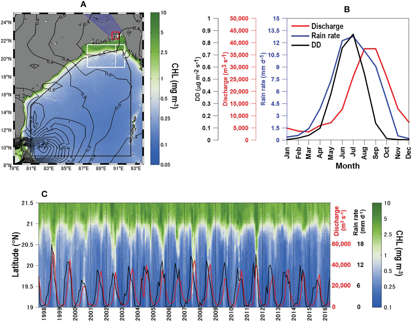
Figure 1 (A) Annual means of satellite-derived CHL (shaded map) overlaid by the SPRINTARS-modeled DD (contour map). The red square indicates the approximate position of the mouth of the GBR. The white rectangle adjacent to the north coast of the bay is the area where CHL was averaged zonally (east-west direction, log scale), and its meridional time series is presented in (C). The red and black solid lines in (C) are time series of GBR discharge and rainfall, respectively. The north-south dashed white line (inside the white box (A) in front of the river mouth) is a transect line where CHL, CHL anomaly, and normalized water-leaving radiance at a wavelength of 555 nm (nLw₅₅₅) were extracted and are presented in Figures 2A–C. (B) Monthly climatological means of DD (black line), rain rate (blue line), and GBR discharge (red line). The DD data were extracted from the region of the BoB bounded by a dashed black polygon in (A). Rainfall data were extracted from the blue hatched polygon in (A), which was part of the catchment area of the GBR.

Because of the upwelled/entrained nutrients from the ocean subsurface layer, CHL is enhanced in the northern summer and peaks in the northern winter, especially over the western/southwestern BoB. Increases in nutrient concentrations that enhance CHL are associated with local longshore wind stress (Shetye et al., 1991; Gomes et al., 2000), westward propagation of upwelling Rossby waves (Rao et al., 2010; Sreenivas et al., 2012; Gulakaram et al., 2018), and strong northeasterly winds (e.g., Xu et al., 2021) during the summer, fall, and winter, respectively.

In addition, the BoB receives large amounts of dust from fallout that also peaks around summer (July) (Figure 1B). Aerosol dust over the BoB is transported from southwest Asia, northeast Asia, and the Middle East (Banerjee and PrasannaKumar, 2016; Banerjee et al., 2019). During summer, a high plume of DD intrudes into the BoB from the southwest (Figure 1A). This plume is attributable to high emissions from dust sources, high rainfall over the BoB, and a slight deflection (southeastward to northeastward) of winds around the southern Indian Peninsula (Banerjee et al., 2019).

2.2 Data sources and analysis

We used satellite-derived monthly CHL blended from multiple ocean color sensors with 4-km resolution downloaded from the ESA OC-CCI (https://esa-oceancolour-cci.org/), monthly sea surface height anomaly (SSHA, cm) with 25-km resolution downloaded from the AVISO+ Satellite Altimetry Data (https://www.aviso.altimetry.fr/), monthly rainfall with 25-km resolution downloaded from the Asia-Pacific Data Research Center (http://apdrc.soest.hawaii.edu/), and daily sea surface temperature (SST, °C) with 4-km resolution retrieved by the Advanced Very High-Resolution Radiometer and downloaded from NOAA (https://www.nodc.noaa.gov/). The daily SST data were then averaged to produce monthly mean SSTs. Variations in SST and SSHA are used widely to assess nutrient inputs from ocean subsurface layers associated with physical processes (e.g., Siswanto, 2015). We also calculated the wind stress curl (curl, N m⁻³) following Large and Pond (1981) from monthly wind fields acquired from the Cross-Calibrated Multi-Platform (CCMP) project (http://podaac.jpl.nasa.gov) as an indicator of upwelling.

We used in situ GBR discharge data acquired from the Bangladesh Water Development Board (https://www.bwdb.gov.bd/) as a proxy for river-borne nutrient input. We used atmospheric DD data as proxies of nutrient inputs from the atmosphere and modeled atmospheric DD using SPRINTARS (Takemura et al., 2003), a numerical model developed by the Research Institute for Applied Mechanics, Kyushu University (https://sprintars.riam.kyushu-u.ac.jp/). We used Nino3.4 as a metric of El Niño/Southern Oscillation (ENSO) variability (http://www.cpc.ncep.noaa.gov/data/indices/sstoi.indices) and the dipole mode index (DMI) as a metric of Indian Ocean Dipole (IOD) variability (http://www.jamstec.go.jp/aplinfo/sintexf/iod/dipole_mode_index.html).

One of the objectives of this study was to determine whether climate variations influence CHL by modulating supplies of nutrients from different sources. Because climate variations have an interannual timescale, the seasonal cycles and long-term trends of CHL and other geophysical variables must be removed from their time series before the effects of changes in sources of nutrients can be detected. To assess whether the ocean subsurface layer or atmospheric deposition was a more important source of inorganic nutrients in different parts of the offshore regions of the BoB, we conducted a multiple linear regression analysis (MLRA) that related CHL to other environmental variables following the approach used by Siswanto (2015) and Nathans et al. (2012). The approach included removing seasonal variations and trends from variables and standardizing them so that they all had means of zero and standard deviations of one. Standardization facilitates the comparison of the importance of one independent variable to that of other variables in determining the variance of CHL. The MLRA required that no data be missing. An empirical, orthogonal function-based data interpolation (e.g., Alvera-Azcarate et al., 2005) was used to fill in missing data in the CHL and SST satellite imageries. Figure S1 in the Supplementary Information shows the numbers and percentages of valid CHL and SST pixels used for interpolation.

3 Results

3.1 Spatial variability of the importance of nutrients from different sources

High CHL in the northern BoB was confined mainly to the area north of ~21°N or within ~200 km offshore of the mouth of the GBR (Figures 1A, C). The time series of meridional CHL variation derived from a meridional transect south of the GBR mouth showed southward dispersion of high CHL during summer, when rainfall intensity and river discharge peak (Figure 2A). Tan et al. (2006) and Siswanto et al. (2011) have reported that CHL in the coastal region is systematically overestimated by satellite-retrieved CHL because of the high concentration of total suspended matter, which is generally quantified by satellite-retrieved normalized water-leaving radiance at a wavelength of 555 nm (nLw₅₅₅). They have found that the variation of satellite-derived CHL in the coastal region can be considered to reflect real variations in phytoplankton biomass if nLw₅₅₅ <2.0 mW cm⁻² µm⁻¹ sr⁻¹.

FIGURE 2

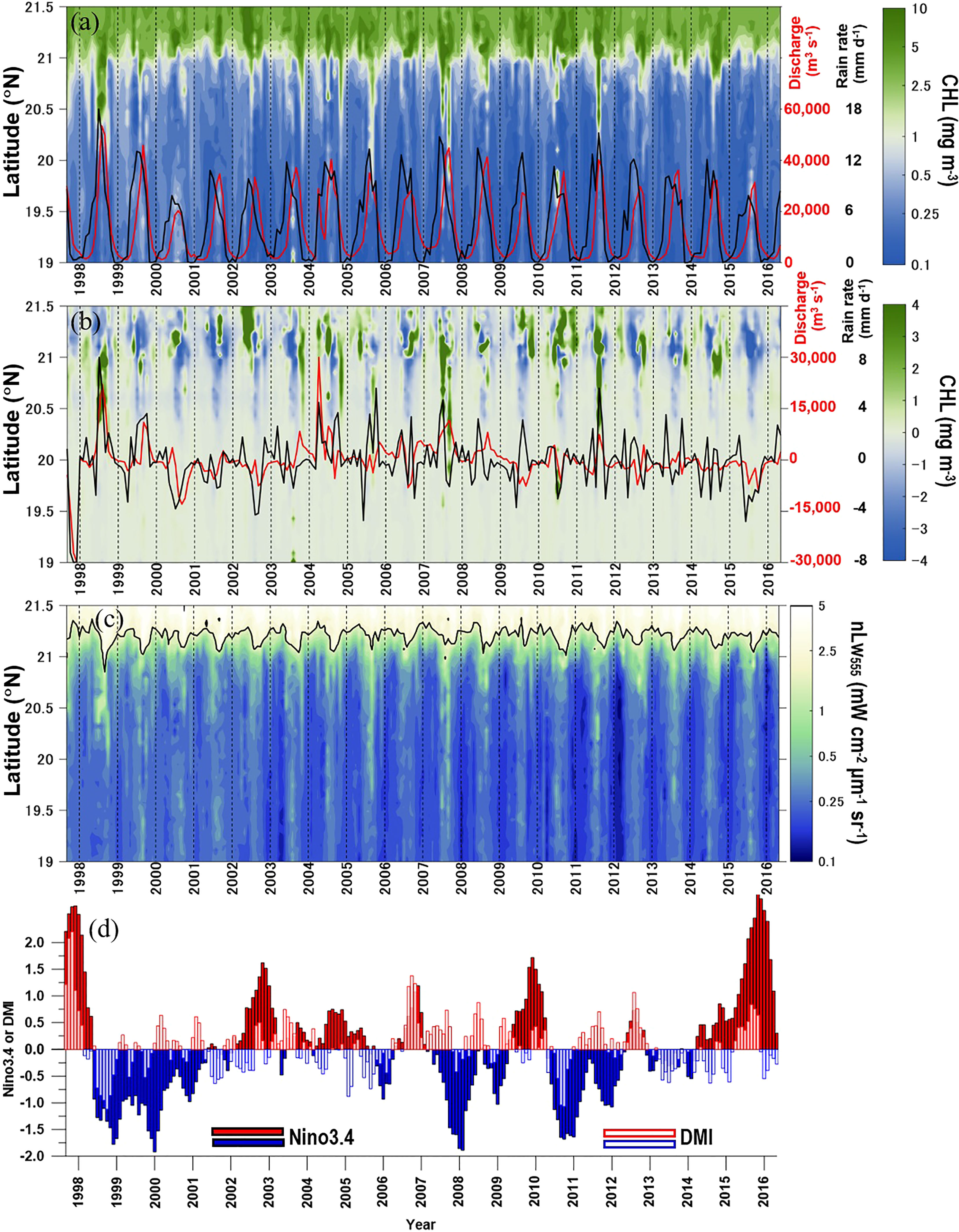
Figure 2 Time series of (A) CHL meridional variations along the white dashed transect line in Figure 1A. Panel (B) is the same as panel (A), except that it shows a CHL anomaly. Panel (C) is the same as panel (A) except that it shows nLw₅₅₅. The red and black lines in (A) are time series of GBR discharge and rain rate, respectively. The red and black lines in (B) show the anomalies in GBR discharge and rain rate. The black contour line in (C) indicates the satellite-retrieved normalized water-leaving radiance at a wavelength of 555 nm (nLw₅₅₅) of 2.5 mW cm⁻² μm⁻¹ sr⁻¹. The time series of Nino3.4 and DMI are shown in (D) to indicate climate variations of the El Niño/Southern Oscillation and Indian Ocean Dipole.

Figure 2C shows temporal variations of nLw₅₅₅ along the meridional transect line off the mouth of the GBR shown in Figure 1A. During the peak discharge of the GBR in summer, the area where the nLw₅₅₅ exceeded 2.0 mW cm⁻² µm⁻¹ sr⁻¹ was confined mainly to the area north of 21°N. Variations of CHL south of 21°N, including the high CHL that is dispersed further southward, can be considered to reflect high phytoplankton biomass due to elevated primary productivity modulated by nutrients from rivers, especially from the GBR.

Along the northern coast of the BoB, nutrients from rivers are likely important for phytoplankton in coastal regions only as far as about 200 km from the river mouths. The distance from the river mouths would depend on the intensity of rainfall and interannual variations of river discharge; thus, CHL variation in the BoB offshore region is likely attributable to variations in other sources of nutrients.

To identify which source of nutrients was most important in determining the offshore variations of CHL in the BoB on an interannual basis, we used a MLRA with CHL as the dependent variable. The independent variables were DD and a physical variable (i.e., CHL = f[SST, DD], CHL = f[SSHA, DD], and CHL = f[curl, DD]). We ran the MLRA with SST, SSHA, and curl independently because variations in SST, SSHA, and curl are not independent but instead are highly dependent on oceanographic physical processes. Figures 3A–C show partial regression coefficients (β) for SST (β_SST), DD (β_DD), and the coefficients of determination (R²) derived from the MLRA of CHL = f(SST, DD). Similarly, Figures 3D–F show the β_SSHA, β_DD, and R² produced by the MLRA of CHL = f(SSHA, DD), and Figures 3G–I show the β_Curl, β_DD, and R² produced by CHL = f(curl, DD). There is much seasonal variability in CHL as well as in the independent variables SST, SSHA, curl, and DD. Prior to running the MLRAs, we removed seasonal cycles and long-term trends from the variables (see Section 2.2) to focus the analysis on interannual variations. Our results therefore concern interannual variability unrelated to seasonal cycles.

FIGURE 3

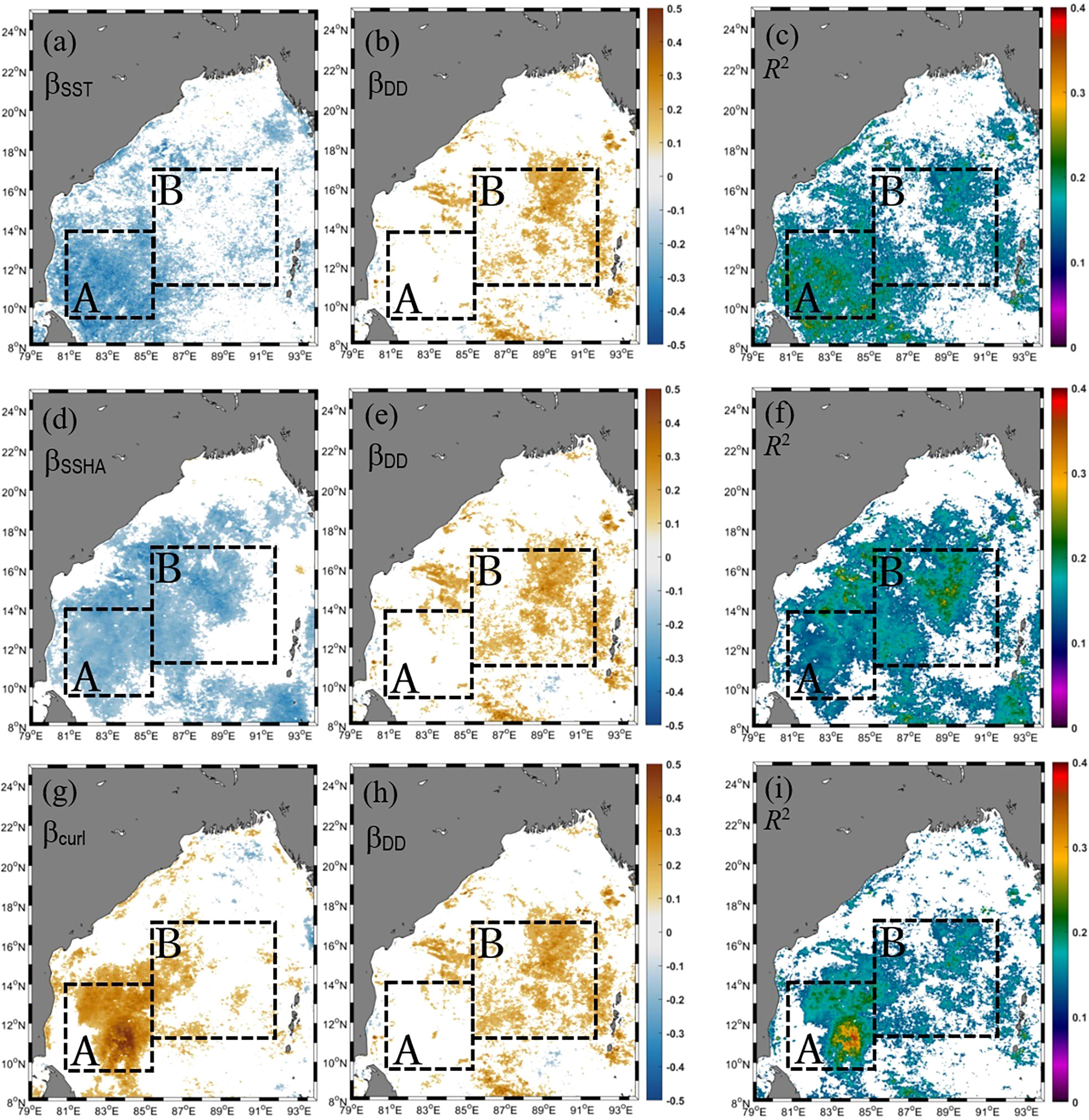
Figure 3 Spatial variations of (A) β_SST, (B) β_DD, and (C) R² obtained from a multiple linear regression analysis with CHL as the dependent variable and SST and dust deposition (DD) as independent variables (i.e., CHL = f[SST, DD]). Panels (D, E), and (F) are the same as (A–C), except that CHL = f(SSHA, DD). Panels (G, H), and (I) are the same, except that CHL = f(curl, DD). Areas where β values were insignificant at the 95% confidence level (p-value >0.05) are masked out (white areas). Yellow (blue) areas in the panels indicate significant positive (negative) associations between CHL and the independent variables. Black dashed box A indicates the part of the southwestern bay where the time series of SST, curl, CHL, and SSHA were extracted from and are presented in Figures 4B, C. The dashed box B indicates the central/eastern bay where the time series of CHL, SST, DD, curl, and SSHA were extracted and are presented in Figures 4D, E.

Negative values of β_SST, which were especially common in the southwestern BoB indicated by box A in Figure 3A, indicated an increase in CHL associated with surface cooling (hence an increase in nutrient concentrations due to upwelling, vertical mixing, or both) (e.g., Shetye et al., 1991; Gomes et al., 2000; Vinayachandran and Mathew, 2003; Martin and Shaji, 2015; Xu et al., 2021). The hypothesis that nutrients introduced from the ocean subsurface layer by upwelling led to increases in CHL in the southwestern part of the bay was also supported by the negative β_SSHA (Figure 3D) and positive β_Curl (Figure 3G). A negative β_SSHA implies that an increase in CHL was associated with a negative SSHA due to upwelling. A positive β_Curl means that an increase in CHL was associated with a positive curl, which is also indicative of upwelling. As shown in Table 1, the values of the mean β_SST (−0.25), mean β_SSHA (−0.20), and mean β_curl (0.26) averaged over box A were larger in magnitude than the mean β_DD (0.14–0.15). The implication is that variations in the supply of nutrients from the ocean subsurface layer contributed more than variations in the supply of nutrients from atmospheric deposition to the interannual variations of CHL in the southwestern BoB. The mean R² (0.15–0.18) resulting from the three MLRAs (Figures 3C, F, I, Table 1) implies that variations in the supply of nutrients from the ocean subsurface layer explain 15%–18% of the interannual variations of CHL in the southwestern BoB.

TABLE 1

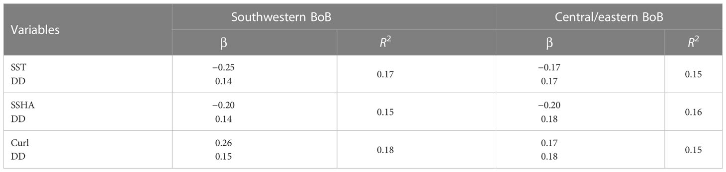
Table 1 Mean values of partial regression coefficients β_SST, β_SSHA, β_curl, and β_DD averaged over the southwestern and central/eastern BoB and their coefficients (R²) in multiple linear regression analyses.

In the central/eastern BoB, nutrients from upwelled/entrained water and atmospheric deposition could together explain about 15% (R² = 0.15–0.16, Table 1) of the interannual variance of CHL. In general, the spatial averages of the mean β_SST (−0.17), mean β_SSHA (−0.20), and mean β_curl (0.17) over box B were comparable with the mean β_DD (0.18–0.19). However, the significant β_DD occurred in different areas (the eastern part of box B) than the significant β_SST, β_SSHA, and β_curl (the western part of box B) (Figures 3A, B, D, E, G, H). It is therefore likely that deposited nutrients are particularly important for phytoplankton in the western part of box B, or in general, in the western part of the bay. The fact that β_SST, β_SSHA, and β_DD were insignificant in the northern coastal region indicates that river-borne inorganic nutrients were likely more important in determining variations of phytoplankton CHL in the central/eastern bay.

3.2 Possible linkages with climate variations

3.2.1 BoB northern coastal region

There is interannual variation over the seasonal cycle of high CHL during summer/fall along the northern coast of the BoB (Figures 1C, 2A). The CHL interannual variation can be seen more obviously in terms of the variation of the meridional CHL anomaly along the meridional transect line (19.0°N–21.5°N, Figure 2B).

Expansions of high-CHL waters further southward (up to about 300 km south of the GBR mouth) were obvious during the summer/fall of 1998, 2005, 2007, and 2011. Those years were characterized by anomalously high rainfall over the catchment area and high discharges from the GBR (Figure 2B). The years 1998, 2005, and 2011 were La Niña years and negative-IOD (nIOD) years (hereafter La Niña/nIOD), whereas 2007 was a La Niña year (Figure 2D).

3.2.2 BoB southwestern region

To assess whether nutrient inputs from the ocean subsurface layer that determine interannual variations of CHL in the southwestern BoB were correlated with climate variations, we plotted time series of CHL, SST, curl, and SSHA along with the Nino3.4 and DMI (Figures 4A–C). In general, CHL varied inversely with SST but positively with curl. Such an inverse relationship between CHL and SST and a positive relationship between CHL and curl can also be seen in the corresponding scatter plots (Figures 5A, B). The correlation coefficients between CHL and SST (−0.43, DF = 224) and between CHL and curl (0.43, DF = 224) were statistically significant (two-tailed t-test, p <0.0001) (Table 2). The negative correlation between CHL and SST indicated that entrained cold (hence nutrient-rich) water was associated with high CHL. The entrainment could have been driven by upwelling and/or vertical mixing. The positive curl would be associated with upwelling or Ekman divergence processes. The positive correlation between CHL and curl therefore indicated that upwelling was the major physical process that entrained nutrients from the ocean’s subsurface layer to enhance CHL.

FIGURE 4

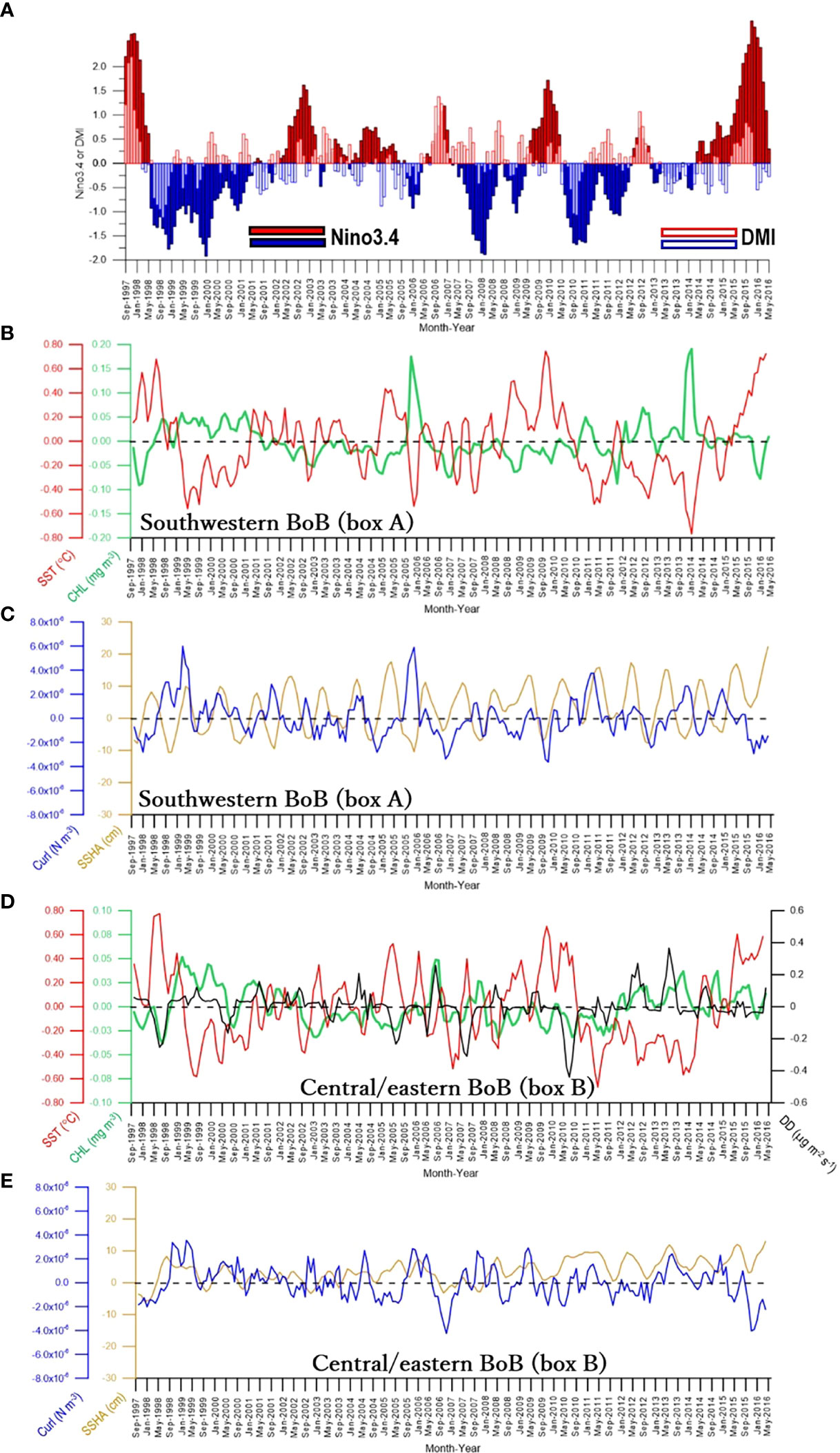
Figure 4 (A) Time series of Nino3.4 (closed bars) and DMI (open bars) to be compared with time series of (B) CHL and SST, and (C) curl and SSHA extracted from box A (see Figure 3) in the southwestern bay. Panels (D, E) are time series of SST, CHL, DD, curl, and SSHA extracted from box B (see Figure 3) in the central/eastern bay.

FIGURE 5

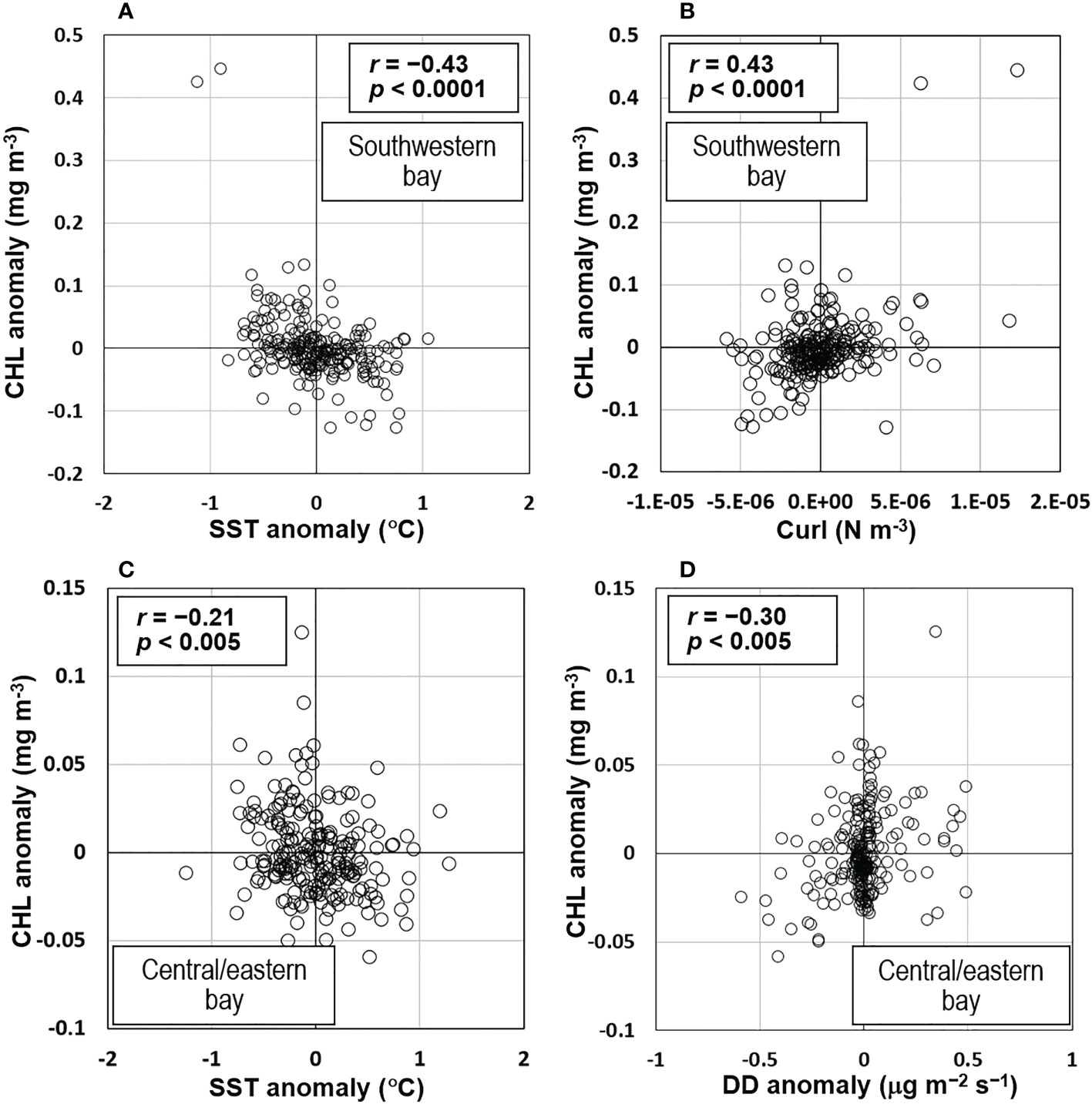
Figure 5 Scatter plots of CHL anomalies versus anomalies of (A) SST and (B) curl derived from the southwestern Bay of Bengal (BoB), and versus anomalies of (C) DD and (D) SST, derived from the central/eastern BoB.

TABLE 2

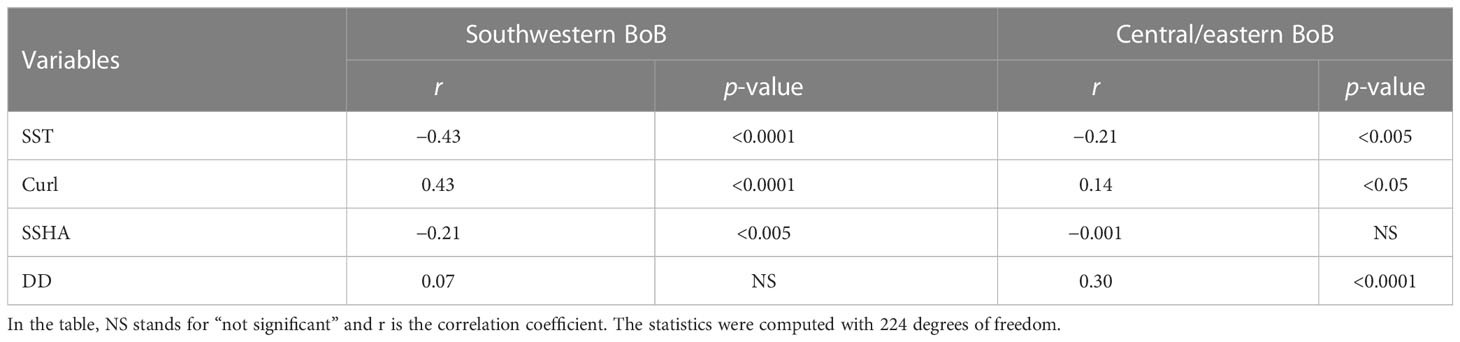
Table 2 Results of regression analysis performed by relating CHL to SST, curl, SSHA, and DD in the southwestern and central/eastern BoB.

Interestingly, in general, the negative correlation between CHL and SST (Figures 4B, 5A) and the positive correlation between CHL and curl (Figures 4B, C, 5B) were likely linked with ENSO, IOD, or both. For instance, negative CHL, positive SST, and negative curl variations were obvious during the concurrent El Niño and positive IOD (hereafter El Niño/pIOD) in 1997, El Niño/pIOD in 2009, and the 2017 El Niño. In contrast, positive CHL, negative SST, and positive curl anomalies were evident during the La Niña/nIOD of 1998, the La Niña of 1999, the La Niña/nIOD of 2005, and the La Niña/nIOD of 2013. This pattern indicates that atmosphere–ocean interactions associated with interannual climate variations of ENSO and IOD drive the supply of inorganic nutrients from the ocean subsurface layer, and an increase in the supply of nutrients (indicated by low SST) to the surface layer leads to increases in CHL.

Compared to SST and curl, SSHA was more weakly correlated with CHL (0.21, DF = 224), but the correlation was still statistically significant (p <0.005) (Table 2). The strong seasonality of SSHA in the BoB is associated with westward-propagating Rossby waves (Sreenivas et al., 2012; Gulakaram et al., 2018) that likely weaken the relationship between CHL and SSHA on an interannual timeframe. Westward-propagating Rossby and coastal Kelvin waves (that traverse along the BoB coast) are generated at the eastern boundary of the BoB. They are feedback from eastward-propagating equatorial Kelvin waves.

3.2.3 BoB central/eastern region

In the central/eastern BoB, the time series of CHL, SST, and DD anomalies show that CHL generally varies inversely with SST but positively with DD. This pattern is apparent in the corresponding scatter plots (Figures 4D, 5C, D). The strongest interannual association was between CHL and DD, for which the correlation coefficient was 0.30 (p <0.0001, DF = 244, Table 2, Figure 5D). CHL and SST were also significantly correlated (r = −0.21, p <0.005, DF = 224, Table 2, Figure 5C). CHL was significantly correlated with curl (r = 0.14, DF = 224) (Figure 4E) but with a lower level of confidence (p <0.05). There was no significant correlation between CHL and SSHA (r = −0.001, p >0.05, DF = 224, Figures 4D, E, Table 2).

Despite the significant correlation between CHL and DD in the central/eastern BoB, neither CHL nor DD was clearly associated with either ENSO or IOD. Neither CHL nor DD were significantly correlated with those climate indices (Table 3). The lack of association between CHL, DD, and variations of climate is likely due to the time lag between the time when the climate event peaked and the time of DD entering the BoB (see Discussion). In contrast, as shown in Table 3, the significant correlations between SSHA and Nino3.4 (r = −0.18), between SSHA and DMI (r = −0.35), between curl and Nino3.4 (r = −0.32), and between curl and DMI (r = −0.20) indicate that curl and SSHA were influenced by both ENSO and IOD.

TABLE 3

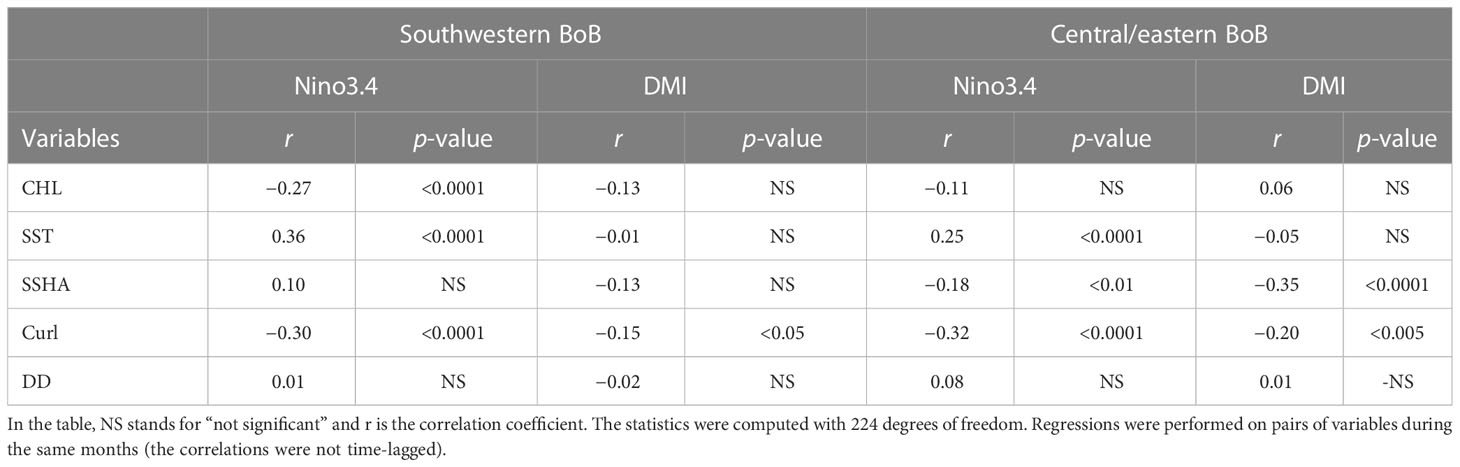
Table 3 Results of regression analysis performed by relating climate indices (Nino3.4, DMI) to CHL, SST, curl, SSHA, and DD in the southwestern and central/eastern BoB.

Climate variations had opposite effects on SSHA and curl (Table 3). The negative correlations between the SSHA and climate indices (Table 3) indicate that El Niño and pIOD led to upwelling, but the negative correlations between the curl and climate indices (Table 3) indicate that they led to downwelling. Regardless of these apparently contradictory relationships, one of the reasons for the lack of association between CHL and climate variations in the central BoB was probably the formation of a freshwater lens associated with the influx of freshwater from river discharge that restricted climate-related atmosphere–ocean interactions (e.g., Kumar et al., 2002; Vinayachandran et al., 2002; Felton et al., 2014; Kay et al., 2018).

4 Factors responsible for anomalously high CHL

Here we will elaborate on the atmosphere-land-ocean interactions that were probably responsible for the remarkably high CHL anomalies in the coastal region of the northern BoB (Figure 2), box A in the southwestern BoB, and box B in the central/eastern BoB (Figure 3). We first discuss the mechanisms responsible for the high CHL in the coastal region, followed by the mechanisms probably responsible for the high CHL in the southwestern and central/eastern BoB.

As reported by Perves and Henebry (2015), the amount of rainfall over the GBR basin increases by more than 100% (compared to the long-term mean rainfall) during years of La Niña alone or La Niña/nIOD. The anomalously high CHL and/or southward dispersion of high-CHL waters along the northern coast of the bay during the La Niña/nIOD or La Niña years of 1998, 2005, 2007, and 2011 can be attributed to high river discharges and hence large influxes of river-borne nutrients associated with La Niña, nIOD, or both. In contrast, during the El Niño years of 1997, 2002, 2009, and 2015, there was no apparent southward dispersion of high-CHL waters (Figures 2A, B) because of the low amounts of rainfall and low river discharges during those El Niño years (Perves and Henebry, 2015). The implication is that there is a teleconnection between basin-scale climate variations of ENSO and/or IOD and land-ocean interaction, i.e., variations of river-borne inorganic nutrient supply and primary production in coastal waters.

Between September 1997 and May 2016, there were two obvious, anomalous peaks of CHL in the southwestern BoB that were accompanied by negative SST, negative SSHA, and positive curl anomalies (Figures 4B, C). The first CHL peak occurred during December 2005 (Figure 6B), a year influenced by La Niña/nIOD (Figure 6A) (see also Li et al., 2017; Chen and Li, 2018). That CHL peak resulted from a spatially large, positive CHL anomaly (Figure 6C-2nd row). That spatially large, positive CHL anomaly was enabled by nutrients supplied from the ocean subsurface layer, as indicated by the positive curl, negative SST, and negative SSHA anomalies (Figure 6C-3rd, 4th, and 5th rows). Previous work has suggested that the high CHL in December 2005 resulted from the passage of cyclones (Ali et al., 2007; Chen et al., 2013; Sridevi et al., 2019). An input of nutrients from the atmosphere is unlikely the explanation for the high CHL because the DD from October 2005 to February 2006 was normal (Figure 6C-1st row), and DD is generally low in December (Figure 1B) (see also Solmon et al., 2015).

FIGURE 6

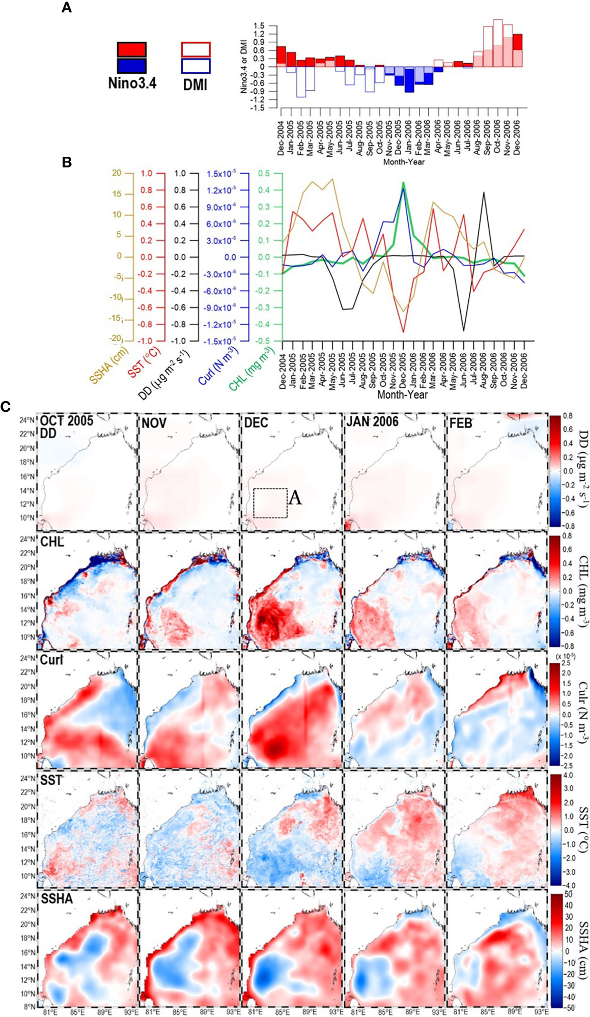
Figure 6 (A) Time series of Nino3.4 and DMI during the period from December 2004 to December 2006. Within that period, panel (B) shows time series of SSHA, SST, DD, curl, and CHL extracted from box A panel (C)-1st row) in the southwestern bay. Panel (C) shows maps of DD (1st row), CHL (2nd row), curl (3rd row), SST (4th row), and SSHA (5th row) for the period from October 2005 to February 2006.

A similar combination of anomalously high CHL accompanied by positive curl, negative SST, and negative SSHA was also apparent in December 2013 (Figures 7B, C-2nd, 3rd, 4th, and 5th rows). These observations indicate that the upwelling of nutrients enhances CHL. Atmospheric inputs were not a cause of the enhancement of CHL because the DD anomalies were negative (Figure 7C-1st row), and December is in the season of low DD (Figure 1B) (Solmon et al., 2015). Oceanographic conditions during this period were also influenced by the 2013 La Niña/nIOD (Figure 7A). Jayaram et al. (2019) have suggested that two cyclones that passed over adjacent areas caused the highest CHL anomaly observed in December 2013.

FIGURE 7

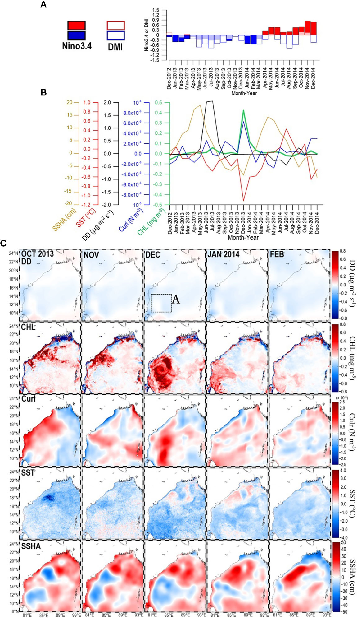
Figure 7 (A) Time series of Nino3.4 and DMI during the period from December 2012 to December 2014. Within that period, panel (B) shows time series of SSHA, SST, DD, curl, and CHL extracted from box A panel (C)-1st row) in the southwestern bay. Panel (C) shows maps of DD (1st row), CHL (2nd row), curl (3rd row), SST (4th row), and SSHA (5th row) for the period from October 2013 to February 2014.

Regardless of the inorganic nutrient composition of DD, the fact that previous studies have shown that increased phytoplankton growth in various ocean basins can be associated with the SPRINTARS-modeled DD (Kitajima et al., 2009; Calil et al., 2011; Fukushima, 2014) indicates that the deposition of inorganic nutrients from the atmosphere is an important source of nutrients for phytoplankton growth. We therefore expected that the SPRINTARS-modeled DD would to some degree alter CHL in the BoB, particularly in the central/eastern bay, where nutrient supplies from river discharge are generally considered to be low. Indeed, we found a significant correlation between CHL and DD in the central/eastern BoB.

However, the role of atmospheric deposition, which is suggested by the significant, positive correlation between CHL and DD (r = 0.30, Table 2), must be interpreted with caution because there was a significant negative (positive) correlation between CHL and SST (CHL and curl) (Table 2); therefore, nutrient inputs from the ocean subsurface layer may also have played an important role. For instance, from May 2012 to May 2014, positive DDs were accompanied not only by positive CHL but also by negative SST (Figure 4D). During this study, only the DD in July–August 2006 likely indicated atmospheric deposition that enhanced CHL in August 2006 (Figures 8B, C-1st and 2nd rows). However, DD might contribute some nutrients because patches of negative SSHA (an indication of upwelling) were observed approximately in the positive CHL areas, though negative curl data indicated downwelling conditions (Figures 8B, C-3rd, 4th, and 5th rows).

FIGURE 8

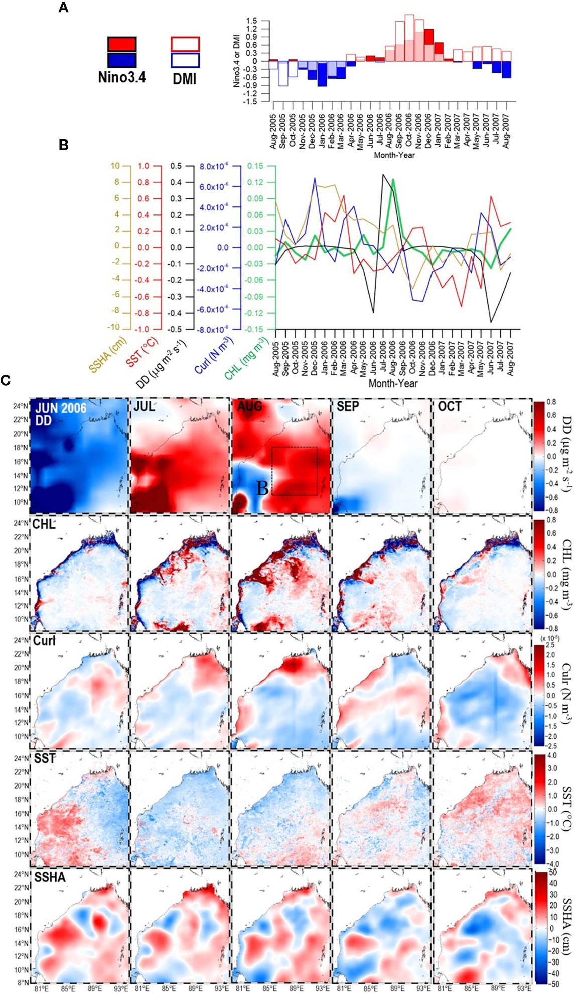
Figure 8 (A) Time series of Nino3.4 and DMI during the period from August 2005 to August 2007. Within that period, panel (B) shows time series of SSHA, SST, DD, curl, and CHL extracted from box B panel (C)-1st row) in the central/eastern bay. Panel (C) shows maps of DD (1st row), CHL (2nd row), curl (3rd row), SST (4th row), and SSHA (5th row) for the period from June 2006 to October 2006.

5 Discussion

In general, CHL in the southwestern BoB was negatively and significantly correlated with Nino3.4 (r = −0.27, p <0.0001, Table 3). CHL therefore tended to be low (high) during El Niño (La Niña). Similarly, there was a negative (but insignificant) correlation between CHL and DMI, i.e., CHL was low (high) during pIOD (nIOD). A similar negative but insignificant CHL–DMI correlation in the southwestern part of the bay has also been reported by Xu et al. (2021). Our analysis indeed showed that ENSO rather than the DMI seemed to have a larger influence on the SST and curl (Table 3). We therefore hypothesize that elucidation of the impacts of climate variations on the biogeophysical variability of the BoB should include consideration of ENSO cycles.

Except for the southwestern BoB, much of the BoB during the La Niña/nIOD period from October 2005 to February 2006 was characterized by a positive SSHA (Figure 6C-5th row). This positive SSHA is known to be associated with a strengthened downwelling Kelvin wave in the equatorial Indian Ocean that is driven by a strong westward wind stress anomaly during La Niña/nIOD (Sreenivas et al., 2012; Roman-Stork et al., 2021). This downwelling equatorial Kelvin wave is reflected westward from the eastern coast of the bay as a downwelling Rossby wave and is characterized by positive SSHA (Rao et al., 2010). However, the SSHA tends to be negative over the southwestern BoB because during La Niña/nIOD, a strong westward wind stress anomaly creates cyclonic wind stress over the southwestern BoB (see Sreenivas et al., 2012).

The 2005 La Niña/nIOD-driven cyclonic wind stress led to the generation of a mesoscale cyclonic eddy over the same area of high CHL in the southwestern BoB (Figures 6C-2nd row, 9A). Previous studies have attributed this high CHL to cyclone Fanoos, which traversed the BoB from 15 to 22 December 2005 (Ali et al., 2007; Sridevi et al., 2019). However, during October–November 2005, before the arrival of cyclone Fanoos, the positive curl and negative SSHA indicated that a mesoscale cyclonic eddy already existed (Figure 6C-3rd and 5th rows; see also Sridevi et al., 2019). An enhancement of CHL was already apparent in October 2005 (Figure 6C-2nd row). An Ekman divergence associated with La Niña/nIOD was already occurring and was likely strengthened by cyclone Fanoos. The result was a pronounced positive CHL anomaly in December 2005. The increase in CHL could not be attributed to atmospheric input of nutrients because the DD was normal during the period from October 2005 to February 2006 (Figure 6C-1st row).

FIGURE 9

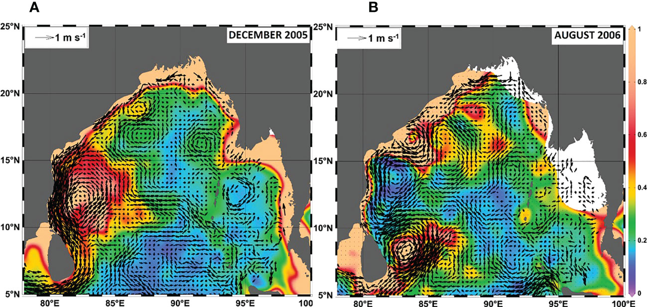
Figure 9 (A) Surface currents estimated by combining surface drifter and altimetry observations following the method of Uchida and Imawaki (2003) and plotted over the CHL in (A) December 2005 and (B) August 2006.

Analysis of the CHL enhancement during the December 2013 La Niña/nIOD requires consideration of the fact that two cyclones passed over the western/southwestern BoB from late November to early December 2013: Cyclone Leher (24–28 November) and Cyclone Madi (5–12 December) (Jayaram et al., 2019). The high CHL in December 2013 (Figures 7B, C-2nd row) was the result of a CHL bloom from 25 November to 2 December 2013 that preceded Cyclone Madi’s arrival (Jayaram et al., 2019). The implication is that Cyclone Madi was not the only driver of the high CHL in December 2013. Although patches of increased CHL along the track of cyclone Leher are apparent in the study of Jayaram et al. (2019), the locations and spatial patterns that show Cyclone Leher-driven Ekman pumping and that show increased CHL are not in the same places. It is therefore unlikely that the CHL bloom in the southwestern BoB was associated with the passage of Cyclone Leher. The positive curl and negative SSHA (Figure 7C-3rd and 5th rows) suggest that a cyclonic eddy already existed in October–November 2013 (see also Sridevi et al., 2019). We therefore suggest that the cyclonic eddy that formed in association with the 2013 La Niña/nIOD and the cyclones may have synergistically enhanced Ekman divergence and produced a prominent, positive CHL anomaly in December 2013. The presence of a cyclonic eddy that preceded cyclone Madi has also been mentioned by Chen et al. (2013) and Chowdhury et al. (2022), but those authors did not discuss the connection between the cyclonic eddy that preceded cyclone Madi and the 2013 La Niña/nIOD.

Mahala et al. (2015) and Roose et al. (2022) have recently mentioned that more cyclones are generated in the BoB during La Niña, nIOD, or both. This pattern is associated with anomalous equatorial westerly winds during La Niña, nIOD, or both that favor cyclone formation. Equatorial westerlies also favor cyclonic eddy formation in the southwestern BoB (see Sreenivas et al., 2012). The above-mentioned synergistic effect of mesoscale cyclonic eddies and tropical cyclones over the southwestern BoB is therefore likely to be more frequent during La Niña, nIOD, or both, and hence the CHL in the southwestern BoB will be greatly enhanced during those times.

The negative anomalies of DD from October 2013 to February 2014 (Figure 7C-1st row) and the seasonal minimum of DD during this period (Figure 1B) (see also Solmon et al., 2015) confirmed that nutrients upwelled from the ocean subsurface layer by climate-driven cyclonic eddies and cyclone passages were the only sources of nutrients that enhanced CHL in December 2013. The enhancements of CHL during the 1998 La Niña/nIOD, 1999 La Niña, and 2010 La Niña/nIOD were less remarkable than the enhancements during the 2005 and 2013 La Niña/nIOD. One reason was that the areas where phytoplankton bloomed during those climatic events were not entirely within the southwestern BoB (maps not shown). The entire CHL bloom was therefore not counted when the CHL within box A was averaged in the southwestern BoB.

Based on field experiments, Yadav et al. (2016) have also mentioned that inorganic nutrients from dust enhance CHL by factors of 1.5–4 in the coastal region of the western BoB. Patches of positive β_DD around western bay coastal areas in our study that were approximately the same as the study area of Yadav et al. (2016) confirmed that phytoplankton production in coastal waters also seemed to be sensitive to atmospheric DD.

We observed no correlations between DD in the central/eastern BoB and climate variations in the same months (no time lag) (Table 3). There may, however, be a time lag between climate variations and DDs (e.g., Banerjee and PrasannaKumar, 2016). To determine whether there was a time lag between climate variations and DDs in the BoB, we investigated the relationship between Nino3.4 and DD with different time lags. Figure 10A shows the correlations and reveals that DDs were highly correlated with Nino3.4 variations that occurred 6–8 months earlier (r <−0.20, p <0.01). The highest correlations were observed with a 7-month lag (Nino3.4 leading, r = −0.24, DF = 217, p <0.005). Interestingly, high correlations between Nino3.4 and CHL (r <−0.20, p <0.01) were also observed with time lags of 6–7 months (Figure 10B).

FIGURE 10

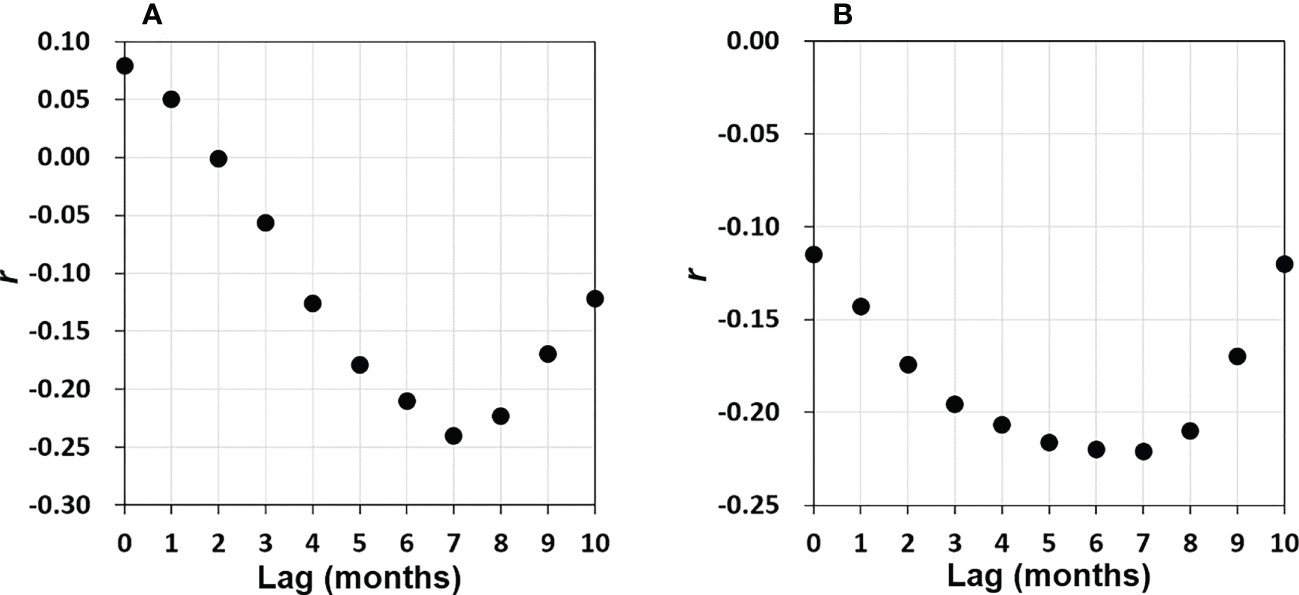
Figure 10 (A) A plot of r (DD anomaly versus Nino3.4) derived from linear regressions with various time lags (months, Nino3.4 leads DD). Panel (B) is the same as panel (A) but for CHL anomaly versus Nino3.4.

The probable explanation for the negative correlations between Nino3.4–DD and Nino3.4 versus CHL 6–7 months later is that La Niña causes anomalously low precipitation in the dust source regions (i.e., southwestern Asia, the Middle East, and Eastern Africa) that leads to more dust generation during the following summer (Banerjee and PrasannaKumar, 2016). High DD that partially enhanced CHL in August 2006 (Figures 8B, C-1st and 2nd rows) was apparent following the 2005 La Niña peak (January, Figure 8A). Similar La Niña–DD lagged co-variations were also apparent for other years: a La Niña peak in December 1998 preceded a DD peak in June 1999; a La Niña peak in January 2008 preceded high DD in May–June 2009; a La Niña peak in December 2011 preceded high DD in June–July 2012; and a La Niña in December 2012 preceded high DD in May–June 2013 (Figures 4A, D). In contrast and consistent with Banerjee and PrasannaKumar (2016), El Niño peaks were followed by low DD in the following summers: an El Niño peak in December 1997 preceded low DD in July 1998, and an El Niño peak in December 2009 preceded a very low DD in July 2010.

Because the deposition of dust generated from the same sources mentioned above is important in determining primary production in the Arabian Sea (Tandule et al., 2022) and because we found a significant correlation between DD and CHL in the central/eastern BoB (r = 0.30, Table 2), we suggest that DD plays an important role in determining primary production in the BoB, especially in the central/eastern bay. In addition, the Nino3.4–DD and Nino3.4–CHL (Figure 10) lagged correlations indicated that ENSO influences DD (and hence CHL) in the BoB 6–8 months after the peak of ENSO.

However, when assessing the impact of DD on CHL in the central/eastern bay, it is important to note that there may also have been a contribution of nutrients from other sources, even during the high DD in August 2006 (Figure 8B, C-1st row). During August, nutrient inputs from the ocean subsurface layer are likely to be limited by the formation of a barrier layer associated with the flux of freshwater from the GBR that restricts climate-related atmosphere–ocean interactions (e.g., Vinayachandran et al., 2002; Felton et al., 2014; Kay et al., 2018). Moderate increases in CHL in the central/eastern BoB (box B) may therefore be largely associated with DD. But episodic cyclonic eddies, such as the eddies that form off the western coast (Figure 9B), may also supply nutrients from the ocean subsurface layer and enhance CHL in the coastal region. Coastal waters with high CHL may be transported into the central/eastern bay by surface circulation. A more quantitative analysis would be required to assess the contributions of nutrients from the atmosphere and ocean subsurface layer separately (e.g., Siswanto, 2015).

Understanding how climate impacts phytoplankton CHL in the BoB by altering nutrient inputs from different sources would be valuable for local fisheries management because fisheries production in the BoB is largely controlled by phytoplankton primary production, and a common metric of phytoplankton production is CHL (Hossain et al., 2020). Climate change may reduce or increase local fisheries production by similarly changing CHL. This report may therefore be used as a reference by fisheries-related stakeholders in planning necessary adaptations to fisheries activities in response to climate change.

6 Conclusions

This study revealed that variations of nutrient inputs (inferred from variations of physical parameters) from different sources (river discharge, ocean subsurface layer, and atmosphere) cause variations of phytoplankton CHL in different parts of the BoB from year to year. Nutrients from the GBR are important for CHL mainly in the coastal region at distances up to ~200 km from the northern coast of the BoB. By increasing the amount of rainfall (hence the supply of river-borne nutrients from the GBR), La Niña can extend high-CHL waters further southward (~300 km from the coast). Variations in the supply of nutrients from the ocean subsurface layer determine interannual variations of phytoplankton CHL, mainly in the southwestern BoB. This variation in nutrient supply is linked with ENSO, IOD, or both through the generation of mesoscale cyclonic eddies during La Niña/nIOD. Such La Niña/nIOD-related mesoscale cyclonic eddies, together with the passage of cyclones, may synergistically intensify Ekman divergence, which results in a pronounced CHL enhancement in the southwestern bay. Nutrients deposited from the atmosphere make a nontrivial contribution to the interannual variations in CHL in the central/eastern BoB. This study also suggests that there is a lag of 6–7 months between the peaks of ENSO and the variations of DD and associated enhancements of CHL in the central/eastern BoB. Because phytoplankton are the base of the marine food web, local fishery production is also expected to be affected by climate variations that modulate CHL.

Data availability statement

Publicly available datasets were analyzed in this study. This data can be found here: https://esa-oceancolour-cci.org/; http://marine.copernicus.eu/; https://www.aviso.altimetry.fr/; https://www.nodc.noaa.gov/; http://apdrc.soest.hawaii.edu/; and http://podaac.jpl.nasa.gov/.

Author contributions

ES conceptualized and led the study. MS assisted with river discharge data acquisition and analysis. BP assisted with ocean surface circulation computation from global drifter and altimetry data. TT modeled and provided atmospheric dust deposition data. TH assisted with discussion concerning climate changes and teleconnection of physical oceanographic process. KM, FT, and MH assisted with discussion on the impacts of atmospheric deposition on ocean primary production. MH assisted with financial support and led the research project. All authors contributed to the article and approved the submitted version.

Funding

This research was financially supported by a Grants-in-Aid for Scientific Research (KAKENHI JP18H04144) from the Ministry of Education, Culture, Sports, Science, and Technology-Japan and by the Climate Adaptation Framework Project (CAF2017-RR02-CMY-Siswanto) funded by the Asia-Pacific Network for Global Change Research.

Acknowledgments

We thank the Ocean Color Climate Change Initiative Project (CHL; https://esa-oceancolour-cci.org/), the Copernicus Marine Environment Monitoring Service (SSHA; http://marine.copernicus.eu/, https://www.aviso.altimetry.fr/), the NASA National Oceanographic Data Center (SST, https://www.nodc.noaa.gov/), the Asia-Pacific Data Research Center (rain rate, http://apdrc.soest.hawaii.edu/), the Cross-Calibrated Multi-Platform project (wind fields, http://podaac.jpl.nasa.gov/), and the Bangladesh Water Development Board (river discharge, https://www.bwdb.gov.bd/) for processing and distributing the primary datasets.

Conflict of interest

The authors declare that the research was conducted in the absence of any commercial or financial relationships that could be construed as a potential conflict of interest.

Publisher’s note

All claims expressed in this article are solely those of the authors and do not necessarily represent those of their affiliated organizations, or those of the publisher, the editors and the reviewers. Any product that may be evaluated in this article, or claim that may be made by its manufacturer, is not guaranteed or endorsed by the publisher.

Supplementary material

The Supplementary Material for this article can be found online at: https://www.frontiersin.org/articles/10.3389/fmars.2023.1052286/full#supplementary-material

Supplementary Figure 1 | (A) Spatial distribution of the total number of CHL valid pixels used for CHL interpolation to fill missing data due to cloud coverage. Note that there were a total of 225 CHL imageries from September 1997 to May 2016. Panel (B) is the same as panel (A), but for valid SST pixels.

References

Ali M. M., Jagadeesh P. S. V., Jain S. (2007). Effects of eddies on bay of Bengal cyclone intensity. EOS 88 (8), 93–95. doi: 10.1029/2007EO080001

CrossRef Full Text | Google Scholar

Alvera-Azcarate A., Barth A., Rixen M., Beckers J. M. (2005). Reconstruction of incomplete oceanographic data sets using empirical orthogonal functions: Application to the Adriatic Sea. Ocean Modell. 9, 325–346. doi: 10.1016/j.ocemod.2004.08.001

CrossRef Full Text | Google Scholar

Banerjee P., PrasannaKumar S. (2016). ENSO modulation of interannual variability of dust aerosols over the Northwest Indian ocean. J. Clim. 29 (4), 1287–1303. doi: 10.1175/JCLI-D-15-0039.1

CrossRef Full Text | Google Scholar

Banerjee P., Satheesh S. K., Moorthy K. K., Nanjundiah R. S., Nair V. S. (2019). Long-range transport of mineral dust to the northeast Indian ocean: Regional versus remote sources and the implications. J. Clim. 32 (5), 1525–1549. doi: 10.1175/JCLI-D-18-0403.1

CrossRef Full Text | Google Scholar

Calil P. H. R., Doney S. C., Yumimoto K., Eguchi K., Takemura T. (2011). Episodic upwelling and dust deposition as bloom triggers in low-nutrient, low-chlorophyll regions. J. Geophys. Res. 116, C6. doi: 10.1029/2010JC006704

CrossRef Full Text | Google Scholar

Chen M., Li T. (2018). Why 1986 El nino and 2005 la Nina evolved different from a typical El nino and la Nina. Clim. Dyn. 51, 4309–4327. doi: 10.1007/s00382-017-3852-1

CrossRef Full Text | Google Scholar

Chen X., Pan D., Bai Y., He X., Chen C. T. A., Hao Z. (2013). Episodic phytoplankton bloom events in the bay of Bengal triggered by multiple forcings. Deep. Res. Part I Oceanogr. Res. Pap. 73, 17–30. doi: 10.1016/j.dsr.2012.11.011

CrossRef Full Text | Google Scholar

Chowdhury R. R., Kumar S. P., Chakraborty A. (2022). A study on the physical and biogeochemical responses of the bay of Bengal due to cyclone madi. J. Oper. Oceanogr. 15 (2), 104–125. doi: 10.1080/1755876X.2020.1817659

CrossRef Full Text | Google Scholar

Dai Y., Trenberth K. E. (2002). Estimates of freshwater discharge from continents: Latitudinal and seasonal variations. J. Hydromet. 3 (6), 660–687. doi: 10.1175/1525-7541(2002)003<0660:eofdfc>2.0.co;2

CrossRef Full Text | Google Scholar

Elayaperumal V., Hermes R., Brown D. (2019). An ecosystem based approach to the assessment and governance of the bay of Bengal Large marine ecosystem. Deep-Sea Res. II 163, 87–95. doi: 10.1016/j.dsr2.2019.01.001

CrossRef Full Text | Google Scholar

Felton C. S., Subrahmanyam B., Murty V. S. N., Shriver J. F. (2014). Estimation of the barrier layer thickness in the Indian ocean using aquarius salinity. J. Geophys. Res. 119 (7), 4200–4213. doi: 10.1002/2013jc009759

CrossRef Full Text | Google Scholar

Fukushima H. (2014). “Variability in mineral dust deposition over the north pacific and its potential impact on the ocean productivity,” in Western Pacific air-Sea interaction study. Eds. Uematsu M., Yokouchi Y., Watanabe Y. W., Takeda S., Yamanaka Y. (Terrapub, Tokyo) 51–60. doi: 10.5047/w-pass.a01.006

CrossRef Full Text | Google Scholar

Gomes H. R., Goes J. I., Saino T. (2000). Influence of physical processes and freshwater discharge on the seasonality of phytoplankton regime in the bay of Bengal. Cont. Shelf Res. 20, 313–330. doi: 10.1016/S0278-4343(99)00072-2

CrossRef Full Text | Google Scholar

Grand M. M., Measures C. I., Hatta M., Hiscock W. T., Buck C. S., Landing W. M. (2015). Dust deposition in the eastern Indian ocean: The ocean perspective from Antarctica to the bay of Bengal. Global Biogeochem. Cycles 29, 357–374. doi: 10.1002/2014GB004898

CrossRef Full Text | Google Scholar

Gulakaram V. S., Vissa N. K., Bhaskaran P. K. (2018). Role of mesoscale eddies on atmospheric convection during summer monsoon season over the bay of Bengal: A case study. J. Ocean Eng. Sci. 3, 343–354. doi: 10.1016/j.joes.2018.11.002

CrossRef Full Text | Google Scholar

Hossain M. S., Sarker S., Sharifuzzaman S. M., Chowdhury S. R. (2020). Primary productivity connects hilsa fishery in the bay of Bengal. Sci. Rep. 10, 5659. doi: 10.1038/s41598-020-62616-5

PubMed Abstract | CrossRef Full Text | Google Scholar

Jayaram C., Bhaskar T. V. S. U., Kumar J. P., Swain D. (2019). Cyclone enhanced chlorophyll in the bay of Bengal as evidenced from satellite and BGC-argo float observations. J. Indian Soc Rem. Sen. 47 (11), 1875–1882. doi: 10.1007/s12524-019-01034-1

CrossRef Full Text | Google Scholar

Kay S., Caesar J., Janes T. (2018). “Marine dynamics and productivity in the bay of Bengal,” in Ecosystem services for well-being in deltas. Eds. Nicholls R., Hutton C., Adger W., Hanson S., Rahman M., Salehin M. (Cham: Palgrave Macmillan). doi: 10.1007/978-3-319-71093-8_14

CrossRef Full Text | Google Scholar

Kitajima S., Furuya K., Hashihama F., Takeda S., Kanda J. (2009). Latitudinal distribution of diazotrophs and their nitrogen fixation in the tropical and subtropical western north pacific. J. Geophys. Res. 54 (2), 537–547. doi: 10.4319/lo.2009.54.2.0537

CrossRef Full Text | Google Scholar

Kumar S. P., Muraleedharan P. M., Prasad T. G., Gauns M., Ramaiah N., De Souza S. N., et al. (2002). Why is the bay of Bengal less productive during summer monsoon compared to the Arabian Sea? Geophys. Res. Lett. 29 (24). doi: 10.1029/2002GL016013

CrossRef Full Text | Google Scholar

Kumar S. P., Narvekar J., Nuncio M., Kumar A., Ramaiah N., Sardesai S., et al. (2010). Is the biological productivity in the bay of Bengal light limited? Curr. Sci. 98 (10), 1331–1339.

Google Scholar

Large W. G., Pond S. (1981). Open ocean momentum flux measurements in moderate and strong winds. J. Phys. Oceanogr. 11, 324–336. doi: 10.1175/1520-0485(1981)011<0324:OOMFMI>2.0.CO:2

CrossRef Full Text | Google Scholar

Levy M., Shankar D., Andre J.-M., Shenoi S. S. C., Durand F., de Boyer Montegut C. (2007). Basin-wide seasonal evolution of the Indian ocean’s phytoplankton blooms. J. Geophys. Res. 112, C12014. doi: 10.1029/2007JC004090

CrossRef Full Text | Google Scholar

Li J., Liang C., Tang Y., Liu X., Lian T., Shen Z., et al. (2017). Impacts of the IOD-associated temperature and salinity anomalies on the intermittent equatorial undercurrent anomalies. Clim. Dyn. 51, 1391–1409. doi: 10.1007/s00382-017-3961-x

CrossRef Full Text | Google Scholar

Mahala B. K., Nayak B. K., Mohanty P. K. (2015). Impacts of ENSO and IOD on tropical cyclone activity in the bay of Bengal. Nat. Hazard 75, 1105–1125. doi: 10.1007/s11069-014-1360-8

CrossRef Full Text | Google Scholar

Martin M. V., Shaji C. (2015). On the eastward shift of winter surface chlorophyll-a bloom peak in the bay of Bengal. J. Geophys. Res. 120, 2193–2211. doi: 10.1002/2014JC010162

CrossRef Full Text | Google Scholar

Nathans L. L., Oswald F. L., Nimon K. (2012). Interpreting multiple linear regression: a guidebook of variable importance. Pract. Assessment Res. Eval. 17 (9). doi: 10.7275/5fex-b874

CrossRef Full Text | Google Scholar

Nixon S. W., Buckley B. A. (2002). ‘A strikingly rich zone’–nutrient enrichment and secondary production in coastal marine ecosystems. Estuaries 25, 782–796. doi: 10.1007/BF02804905

CrossRef Full Text | Google Scholar

Nixon S., Thomas A. (2001). On the size of the Peru upwelling ecosystem. Deep-Sea Res. I 48, 2521–2528. doi: 10.1016/S0967-0637(01)00023-1

CrossRef Full Text | Google Scholar

Perves M. S., Henebry G. M. (2015). Spatial and seasonal response of precipitation in the Ganges and Brahmaputra river basins to ENSO and Indian ocean dipole modes: implications for flooding and drought. Nat. Hazards Earth Syst. Sci. 15, 147–162. doi: 10.5194/nhess-15-147-2015

CrossRef Full Text | Google Scholar

Rao R. R., Girish Kumar M. S., Ravichandran M., Rao A. R., Gopalakrishna V. V., Thadathil P. (2010). Interannual variability of kelvin wave propagation in the wave guides of the equatorial Indian ocean, the coastal bay of Bengal and the southeastern Arabian Sea during 1993-2006. Deep. Res. Part I Oceanogr. Res. Pap. 57, 1–13. doi: 10.1016/j.dsr.2009.10.008

CrossRef Full Text | Google Scholar

Roman-Stork H. L., Subrahmanyam B., Trott C. B. (2021). Mesoscale eddy variability and its linkage to deep convection over the bay of Bengal using satellite altimetric observations. Adv. Space Res. 68 (2), 378–400. doi: 10.1016/j.asr.2019.09.054

CrossRef Full Text | Google Scholar

Roose S., Ajayamohan R. S., Ray P., Mohan P. R., Mohanakumar K. (2022). ENSO influence on bay of Bengal cyclogenesis confined to low latitudes. NPJ Clim. Atmos. Sci. 5 (31). doi: 10.1038/s41612-022-00252-8

CrossRef Full Text | Google Scholar

Shetye S. R., Shenoi S. S. C., Gouveia A. D., Michael G. S., Sundar D., Nampoothiri G. (1991). Wind-driven coastal upwelling along the western boundary of the bay of Bengal during the southwest monsoon. Cont. Shelf Res. 11 (11), 1397–1408. doi: 10.1016/0278-4343(91)90042-5

CrossRef Full Text | Google Scholar

Siswanto E. (2015). Atmospheric deposition – another source of nutrients enhancing primary productivity in the eastern tropical Indian ocean during positive Indian ocean dipole phases. Geophys. Res. Lett. 42 (13), 5378–5386. doi: 10.1002/2015GL064188

CrossRef Full Text | Google Scholar

Siswanto E., Tang J., Yamaguchi H., Ahn Y.-H., Ishizaka J., Yoo S., et al. (2011). Empirical ocean-color algorithms to retrieve chlorophyll-a, total suspended matter, and colored dissolved organic matter absorption coefficient in the yellow and East China seas. J. Oceanogr. 67 (5), 627–650. doi: 10.1007/s10872-011-0062-z

CrossRef Full Text | Google Scholar

Siswanto E., Sarker M. D. L., Peter B. N. (2022). Spatial variability of nutrient sources determining phytoplankton Chlorophyll-a concentrations in the Bay of Bengal. APN Sci. Bull. 12 (1), 66–74. doi: 10.30852/sb.2022.1834

CrossRef Full Text | Google Scholar

Solmon F., Nair V. S., Mallet M. (2015). Increasing Arabian dust activity and the Indian summer monsoon. Atmos. Chem. Phys. 15, 8051–8064. doi: 10.5194/acp-15-8051-2015

CrossRef Full Text | Google Scholar

Sreenivas P., Gnanaseelan C., Prasad K. V. S. R. (2012). Influence of El niño and Indian ocean dipole on sea level variability in the bay of Bengal. Glob. Planet. Change 80–81, 215–225. doi: 10.1016/j.gloplacha.2011.11.001

CrossRef Full Text | Google Scholar

Sridevi B., Srinivasu K., Bhavani T. S. D., Prasad K. V. S. R. (2019). Extreme events enhance phytoplankton bloom in the south-western bay of Bengal. Indian J. Geo Mar. Sci. 48 (02), 253–258.

Google Scholar

Takemura T., Nakajima T., Higurashi A., Ohta S., Sugimoto N. (2003). Aerosol distributions and radiative forcing over the Asia pacific region simulated by spectral radiation-transport model for aerosol species (SPRINTARS). J. Geophys. Res.: Atmos. 108 (D23). doi: 10.1029/2002JD003210

CrossRef Full Text | Google Scholar

Tan C. K., Ishizaka J., Matsumura S., Yusoff F., Mohamed M. (2006). Seasonal variability of SeaWiFS chlorophyll a in the malacca straits in relation to Asian monsoon. Cont. Shelf Res. 26 (2), 168–178. doi: 10.1016/j.csr.2005.09.008

CrossRef Full Text | Google Scholar

Tandule C. R., Gogoi M. M., Kotalo R. G., Babu S. S. (2022). On the net primary productivity over the Arabian Sea due to the reduction in mineral dust deposition. Sci. Rep. 12, 7761. doi: 10.1038/s41598-022-11231-7

PubMed Abstract | CrossRef Full Text | Google Scholar

Uchida H., Imawaki S. (2003). Eulerian mean surface velocity field derived by combining drifter and satellite altimeter data. Geophys. Res. Lett. 30 (5), 1229. doi: 10.1029/2002GL016445

CrossRef Full Text | Google Scholar

Vinayachandran P. N. (2009). “Impact of physical processes on chlorophyll distribution in the bay of Bengal” in Indian Ocean biogeochemical processes and ecological variability. Eds. Wiggert J. D., Hood R. R., Naqvi S. W. A., Brink K. H., Smith S. L.. (AGU, Washington, D.C.) 185. doi: 10.1029/2008GM000705

CrossRef Full Text | Google Scholar

Vinayachandran P. N., Mathew S. (2003). Phytoplankton bloom in the bay of Bengal during the northeast monsoon and its intensification by cyclones. Geophys. Res. Lett. 33 (11), 1572. doi: 10.1029/2002GL016717

CrossRef Full Text | Google Scholar

Vinayachandran P. N., Murty V. S. N., Ramesh Babu V. (2002). Observations of barrier layer formation in the bay of Bengal during summer monsoon. J. Geophys. Res.: Oceans 107 (C12). doi: 10.1029/2001JC000831

CrossRef Full Text | Google Scholar

Xu Y., Wu Y., Wang H., Zhang Z., Li J., Zhang J. (2021). Seasonal and interannual variabilities of chlorophyll across the eastern equatorial Indian ocean and bay of Bengal. Prog. Oceanogr. 198, 102661. doi: 10.1016/j.pocean.2021.102661

CrossRef Full Text | Google Scholar

Yadav K., Sarma V. V. S. S., Rao D. B., Kumar M. D. (2016). Influence of atmospheric dry deposition of inorganic nutrients on phytoplankton biomass in the coastal bay of Bengal. Mar. Chem. 187, 25–34. doi: 10.1016/j.marchem.2016.10.004

CrossRef Full Text | Google Scholar